GLL-based Context-Free Path Querying for Neo4j

Abstract.

We propose GLL-based context-free path querying algorithm which handles queries in Extended Backus-Naur Form (EBNF) using Recursive State Machines (RSM). Utilization of EBNF allows one to combine traditional regular expressions and mutually recursive patterns in constraints natively. The proposed algorithm solves both the reachability-only and the all-paths problems for the all-pairs and the multiple sources cases. The evaluation on real-world graphs demonstrates that utilization of RSMs increases performance of query evaluation. Being implemented as a stored procedure for Neo4j, our solution demonstrates better performance than a similar solution for RedisGraph. Performance of our solution of regular path queries is comparable with performance of native Neo4j solution, and in some cases our solution requires significantly less memory.

1. Introduction

Context-free path querying (CFPQ) allows one to use context-free grammars to specify constraints on paths in edge-labeled graphs. Context-free constraints are more expressive than the regular ones (RPQ) and can be used for graph analysis in such areas as bioinformatics (hierarchy analysis (Zhang et al., 2016), similarity queries (Sevon and Eronen, 2008)), data provenance analysis (Miao and Deshpande, 2019), static code analysis (Zheng and Rugina, 2008; Rehof and Fähndrich, 2001). Although a lot of algorithms for CFPQ were proposed, poor performance on real-world graphs and bad integration with real-world graph databases and graph analysis systems still are problems which hinder the adoption of CFPQ.

The problem with the performance of CFPQ algorithms in real-world scenarios was pointed out by Jochem Kuijpers (Kuijpers et al., 2019) as a result of an attempt to extend Neo4j graph database with CFPQ. Several algorithms, based on such techniques as LR parsing algorithm (Santos et al., 2018), dynamic programming (Hellings, 2014), LL parsing algorithm (Medeiros et al., 2018), linear algebra (Azimov and Grigorev, 2018), were implemented using Neo4j as a graph storage and evaluated. None of them was performant enough to be used in real-world applications.

Since Jochem Kuijpers pointed out the performance problem, it was shown that linear algebra based CFPQ algorithms, which operate over the adjacency matrix of the input graph and utilize parallel algorithms for linear algebraic operations, demonstrate good performance (Terekhov et al., 2020). Moreover, the matrix-based CFPQ algorithm is a base for the first full-stack support of CFPQ by extending RedisGraph graph database (Terekhov et al., 2020).

However, adjacency matrix is not the only possible format for graph representation, and data format conversion may take a lot of time, thus it is not applicable in some cases. As a result, the development of a performant CFPQ algorithm for graph representations not based on matrices and its integration with real-world graph databases is still an open problem. Moreover, while the all pairs context-free constrained reachability is widely discussed in the community, such practical cases as the all-paths queries and the multiple sources queries are not studied enough.

Additionally, almost the all existing solutions provide algorithms for reachability-only problem. Recently, Jelle Helligs in (Hellings, 2020) and Rustam Azimov in (Azimov et al., 2021) proposed algorithms which allow one to extract paths satisfied specified context-free constraints. The ability to extract paths of interest is important for some applications where the user wants to know not only the fact that one vertex is reachable from another, but also to get a detailed explanation why this vertex is reachable. One of such application is a program code analysis where the fact is a potential problem in code, and paths can help to analyze and fix this problem. While utilization of general-purpose graph databases for code analysis gaining popularity (Rodriguez-Prieto et al., 2020), CFPQ algorithms which provide structural representation of paths are not studied enough.

It was shown that the generalized LL (GLL) parsing algorithm can be naturally generalized to CFPQ algorithm (Grigorev and Ragozina, 2017). Moreover, this provides a natural solution not only for the reachability-only problem but also for the all-paths problem. At the same time, there exists a high-performance GLL parsing algorithm (Afroozeh and Izmaylova, 2015) and its implementation in Iguana project.

Additionally, pure context-free grammars in Backus-Naur Form (BNF) are too verbose to express complex constraints. But almost the all algorithms require query to be in such form. At the same time, Extended Backus-Naur Form (EBNF) can be used to specify context-free languages. EBNF allows combining typical regular expressions with mutually recursive rules which required to specify context-free languages. That does EBNF more user-friendly. But there are no CFPQ algorithms that utilize EBNF for query specification.

In this paper, we generalize the GLL parsing algorithm to handle queries in EBNF without its transformation. We show that it allows to increase performance of query evaluation. Also integrate our solution with the Neo4j graph database and evaluate it. So, we make the following contributions in the paper.

• We propose the GLL-based CFPQ algorithm which can handle queries in Extended Backus-Naur Form without transformation. Our solution utilizes Recursive State Machines (RSM) (Alur et al., 2005) for it. The proposed algorithm can be used to solve both reachability-only and all-paths problems.

• We provide an implementation of the proposed CFPQ algorithm. By experimental study on real-world graphs we show that utilization of RSM-s allows one to increase performance of query evaluation.

• We integrate the implemented algorithm with Neo4j by providing a respective stored procedure that can be called from Cypher. Currently, we use Neo4j as a graph storage and do not extend Cyper to express context-free path patterns. So, expressive power of our solution is limited: we can not use full power of Cypher inside our constrains. Implementing a query language extension amounts to a lot of additional effort and is a part of future work.

• We evaluate the proposed solution on several real-world graphs. Our evaluation shows that the proposed solution in order of magnitude faster than similar linear algebra based solution for RedisGraph. Moreover, we show that our solution is compatible with native Neo4j solution for RPQs, and in some cases requires significantly less memory. Note that while Cypher expressively is limited, our solution can handle arbitrary RPQs.

The paper has the following structure. In section 2 we introduce basic notions and definitions from graph theory and formal language theory. Then, in section 3 we introduce recursive state machines and provide example of CFPQ evaluation using naïve strategy which may leads to infinite computations. Section 4 contains description GLL-based CFPQ evaluation algorithm which uses RSM and solves problems of naïve strategy from the previous section: the algorithm always terminates, can build finite representation of all paths of interest. Section 5 introduces a data set (both graphs and queries) which will be used further for experiments. Further, in section 6 we use this data set to compare different versions of GLL-based CFPQ algorithm. After that, in section 7 we provide details on integration of the best version into Neo4j graph database, and evaluate our solution on the data set introduced before. Related work discussed in section 8. Final remarks and conclusion provided in section 9.

2. Preliminaries

In this section, we introduce basic definitions and notations for graphs, regular languages, context-free grammars, and finally, we formulate variants of the FLPQ problem.

We use a directed edge-labelled graph as a data model. We denote a graph as $D=\langle V,E,L\rangle$, where $V$ is a finite set of vertices, $E\subseteq V\times L\times V$ is a set of edges, and $L$ is a set of edge labels. A path $\pi$ in a graph $D$ is a sequence of edges: $u\xrightarrow{l_{0}}\ldots\xrightarrow{l_{m}}v$. We denote a path between vertices $u$ and $v$ as $u\pi v$. The function $\omega$ maps a path to a word by concatenating the labels of its edges:

(1) $$\omega(\pi)=\omega(u\xrightarrow{l_{0}}\ldots\xrightarrow{l_{m}}v)=l_{0}\ldots l_{m}.$$

In the context of formal languages, we would like to remind the reader of some fundamental facts about regular expressions and regular languages.

Definition 2.1.

A regular expression over the alphabet $\Sigma$ specifies a regular language using the following syntax.

• If $t\in\Sigma$, then $t$ is a regular expression.

• The concatenation $E_{1}\cdot E_{2}$ of two regular expressions $E_{1}$ and $E_{2}$ is a regular expression. Note that in some cases $\cdot$ may be omitted.

• The union $E_{1}\mid E_{2}$ of two regular expressions $E_{1}$ and $E_{2}$ is a regular expression.

• The Kleene star $E^{*}=\bigcup_{n=0}^{n=\infty}R^{n}$ of a regular expression $E$ is a regular expression.

In some cases $E^{+}$ can be used as syntactic sugar for $E\cdot E^{*}$.

Both regular expressions and finite automata specify regular languages and can be converted into each other. Every regular language can be specified using deterministic finite automata without $\varepsilon$-transitions. Note that regular languages form a strong subset of context-free languages.

Definition 2.2.

A context-free grammar is a 4-tuple $G=\langle\Sigma,\mathcal{N},P,S\rangle$, where $\Sigma$ is a finite set of terminals, $\mathcal{N}$ is a finite set of nonterminals, $S\in N$ is the start nonterminal, and $P$ is a set of productions. Each production has the following form: $N_{i}\to w$, where $N_{i}\in\mathcal{N}$ is the left-hand side of the production, and $w\in(\Sigma\cup\mathcal{N})^{*}$ is the right-hand side of the production.

For simplicity, $S\to w_{1}\mid w_{2}$ is used instead of $S\to w_{1};S\to w_{2}$. Some example grammars are presented in equations 22, 21, and 23.

Definition 2.3.

A derivation step (in the grammar $G=\langle\Sigma,\mathcal{N},P,S\rangle$) is a production application: having a sequence of form $w_{1}N_{0}w_{2}$, where $N_{0}\in\mathcal{N}$ and $w_{1},w_{2}\in(\Sigma\cup\mathcal{N})^{*}$, and a production $N_{0}\to w_{3}$, one gets a sequence $w_{1}w_{3}w_{2}$, by replacing the left-hand side of the production with its right-hand side.

Definition 2.4.

A word $w\in\Sigma^{*}$ is derivable in the grammar $G=\langle\Sigma,\mathcal{N},P,S\rangle$ if there is a sequence of derivation steps such that the initial sequence is the start nonterminal of the grammar and $w$ is a final sequence: $S\to w_{1}\to\ldots\to w$, or $S\to^{*}w$.

Definition 2.5.

The language specified by the context-free grammar $G=\langle\Sigma,\mathcal{N},P,S\rangle$ (denoted $\mathcal{L}(G)$) is a set of words derivable from the start nonterminal of the given grammar: $\mathcal{L}(G)=\{w\mid S\to^{*}w\}$.

Definition 2.6.

A context-free grammar $G=\langle\Sigma,\mathcal{N},P,S\rangle$ is in Extended Backus-Naur Form (EBNF) if productions have the form $\mathcal{N}\to E$ where $E$ is a regular expression over $\mathcal{N}\cup\Sigma$.

Grammar in EBNF can be converted Backus-Naur Form, but such transformation requires introducing new productions and new nonterminals that leads to a significant increase in the size of the grammar and, subsequently, poor performance of path querying algorithms.

We use a generalization of a parse tree to represent the result of a query.

Definition 2.7.

Parse tree of the sequence $w$ w.r.t. the context-free grammar $G=\langle\Sigma,\mathcal{N},P,S\rangle$ in EBNF is a rooted, node-labelled, ordered tree where:

• All leaves are labelled with the elements of $\Sigma\cup\{\varepsilon\}$, where $\varepsilon\notin\Sigma\cup\mathcal{N}$ is a special symbol to demote the empty string. Left-to-right concatenation of leaves forms $w$.

• All other nodes are labelled with the elements of $\mathcal{N}$.

• The root is labelled with $S$.

• Let $w_{0}$ is an ordered concatenation of labels of node labelled with $N_{i}$. Then $w_{0}\in\mathcal{L}(r)$, where $N_{i}\to r\in P$.

A set of problems for the graph $D$ and the language $\mathcal{L}$ can be formulated:

(2) $$R =\{(u,v)\mid\text{exists a path }u\pi v\text{ in }D,\omega(\pi)\in\mathcal{L}\}$$

(3) $$Q =\{\pi\mid\text{exists a path }u\pi v\text{ in }D,\omega(\pi)\in\mathcal{L}\}$$

(4) $$R(I) =\{(u,v)\mid\text{exists a path }u\pi v\text{ in }D,u\in I,\omega(\pi)\in\mathcal{L}\}$$

(5) $$Q(I) =\{\pi\mid\text{exists a path }u\pi v\text{ in }D,u\in I,\omega(\pi)\in\mathcal{L}\}$$

Here 2 is the all-pairs reachability problem, and 3 is the all-pairs all-paths problem. The additional parameter $I$ denotes the set of start vertices in 4 and 5. Thus 4 and 5 — are the multiple source reachability and the multiple source all-paths problems respectively. Note, that for the all-paths problems, the result $Q$ can be an infinite set. Typically, the algorithms for these problems build a finite structure which contains all paths of interest, not the explicit set of paths. As far as the intersection of a regular and a context-free language is context-free (Bar-Hillel et al., 1961), the mentioned finite representation of the result for reachability problem is a representation of a context-free language.

This work is focused on a context-free language. In some cases, the language can be regular, but not context-free. This corresponds to two specific cases of formal lqnguage path querying (FLPQ): Context-Free Path Querying (CFPQ) and Regular Path Querying (RPQ).

3. Recursive State Machines

Recursive state machine or RSM (Alur et al., 2005) is a way to represent context-free languages in a way resembling finite automata. It allows us to use a graph-based representation of context-free languages specification and unify the processing of regular and context-free languages. We will use the following definition of RSM in this work.

Definition 3.1.

Recursive state machine (RSM) is a tuple $\mathcal{R}=\langle\mathcal{N},\Sigma,B,B_{S},Q,Q_{S}\rangle$ where

• $N$ is a set of nonterminal symbols,

• $\Sigma$ is a set of terminal symbols,

• $Q$ is a set of states of the RSM,

• $Q_{S}$ is a set of the start states of all boxes,

• $B=\{B_{N_{i}}\mid N_{i}\in\mathcal{N}\}$ is a set of boxes, where each
  $B_{N_{i}}=\langle Q_{N_{i}},q_{S},Q_{F}^{N_{i}},\delta\rangle$ is a deterministic finite automaton without $\varepsilon$-transitions called a box. Here:

  • $Q_{N_{i}}\subseteq Q$ is a set of states of the box,

  • $q_{S}\in Q_{N_{i}}\cap Q_{S}$ is the start state of the box,

  • $Q_{F}^{N_{i}}\subseteq Q_{N_{i}}$ is a set of final states of the box,

  • $\delta\subseteq Q_{N_{i}}\times(\Sigma\cup Q_{S})\times Q_{N_{i}}$ is a transition function of the box.

• $B_{S}\in B$ is the start box of the RSM.

Thus, RSM is a set of deterministic finite state machines without $\varepsilon$-transitions over the alphabet $\Sigma\cup Q_{S}$. But the computation process of RSM differs from the one of DFA because it involves using a stack to handle transitions labelled with elements of $Q_{S}$.

We can use RSM to compute the reachable vertices in a graph. To describe the current state of the computation, we use configurations. Computation can be defined as a transition between configurations.

Definition 3.2.

A Configuration $C_{\mathcal{R}}$ of the computation of the RSM $\mathcal{R}=\langle\mathcal{N},\Sigma,B,B_{S},Q,Q_{S}\rangle$ over the graph $D=\langle V,E,L\rangle$ is a tuple $(q,v,\mathcal{S})$ where

• $q\in Q$ is a current state of RSM,

• $\mathcal{S}$ is the current stack, whose frames have one of two types:

  • return addresses frame (elements of $Q$) to specify states to continue computation after the call is finished;

  • parsing tree node to store fragments of a parsing tree,

• $v\in V$ is the current vertex (current position in the input).

Definition 3.3.

A transition step of the RSM specifies how to get new configurations of RSM, given the current configuration. $C_{\mathcal{R}}\vdash W$ denotes that $\mathcal{R}$ can go to each configuration in $W$ from the configuration $C_{\mathcal{R}}$.

$$(q,v,w_{0}::s::\mathcal{S})\vdash \{(q^{\prime},v^{\prime},t::w_{0}::s::\mathcal{S})\mid(q,t,q^{\prime})\in\delta,(v,t,v^{\prime})\in E\}$$

$$\cup\{(s^{\prime},v,q^{\prime}::w_{0}::s::\mathcal{S})\mid(q,s^{\prime},q^{\prime})\in\delta,s^{\prime}\in Q_{S}\}$$

$$\cup\{(s,v,\textit{Node}(N_{i},w_{0})::\mathcal{S})\mid q\in Q_{F}^{N_{i}}\}$$

where $w_{0}$ is a possibly empty sequence of terminals and nonterminal nodes.

To simplify the acceptance condition, we introduce the concept of an extended RSM.

Definition 3.4.

For the given RSM $\mathcal{R}=\langle\mathcal{N},\Sigma,B,B_{S},Q,Q_{S}\rangle$, the extended RSM

$$\mathcal{R}^{\prime}=\langle\mathcal{N}\cup\{S^{\prime}\},\Sigma\cup\{\$\},B\cup{B^{\prime}_{S}},B^{\prime}_{S},Q\cup\{q_{0}^{\prime},q_{1}^{\prime},q_{2}^{\prime}\},Q_{S}\cup\{q_{0}^{\prime}\}\rangle$$

is an RSM which defines the same language and is built from $\mathcal{R}$ by adding a new start box

$$B^{\prime}_{S}=\langle\{q_{0}^{\prime},q_{1}^{\prime},q_{2}^{\prime}\},q_{0}^{\prime},\{q_{2}^{\prime}\},\{(q_{0}^{\prime},q_{0},q_{1}^{\prime}),(q_{1}^{\prime},\$,q_{2}^{\prime})\}\rangle$$

where

• $q_{0}$ is a start state of $B_{S}$,

• $ is a special symbol to mark the end of input, $\$\notin\Sigma$,

• $q_{i}^{\prime}$ are newly added states, $q_{i}^{\prime}\notin Q$.

Finally, for the given extended RSM $\mathcal{R}$ and the given graph $D$ we say that $v_{n}$ is reachable from $v_{0}$ w.r.t. $\mathcal{R}$ if $(q^{\prime}_{0},v_{0},[])\vdash^{*}C$ such that $(q^{\prime}_{1},v_{n},[N_{S}])\in C$, where $\vdash^{*}$ denotes zero or more transition steps, and $N_{S}$ is a node for the start nonterminal of the original (not extended) RSM. Additionally, $N_{S}$ represents a respective path.

Now we need a way to compute transitions and to build trees efficiently, avoiding recomputation and infinite cycles that are possible with the naive implementation. Moreover, we need a compact representation of all paths of interest whose number can be infinite.

3.1. Example

Figure 1. Extended RSM for grammar $S\to a\ b\mid a\ S\ b$

Figure 2. Input graph

In this section, we introduce a step-by-step example of the context-free constrained path querying using RSM and the naive computation strategy.

Suppose that the input is a graph $D$ presented in figure 2 and the grammar $G$ has two productions $S\to a\ b\mid a\ S\ b$. The start vertex is $v_{0}$ and our goal to find at least one path to each reachable vertex (w.r.t. $G$). The extended RSM for the given grammar is presented in figure 1.

The initial configuration is $(q_{4},v_{0},[])$: we start from the initial state of the box for $S^{\prime}$, the initial position in the graph is a start vertex $v_{0}$, the stack is empty. In each step, we apply rules from definition 3.3 to compute new configurations. The sequence of transitions, presented below, allows us to find a path

$$v_{0}\xrightarrow{a}v_{0}\xrightarrow{b}v_{1}$$

from $v_{0}$ to $v_{1}$ (step 5) and a path

$$v_{0}\xrightarrow{a}v_{0}\xrightarrow{a}v_{0}\xrightarrow{b}v_{1}\xrightarrow{b}v_{0}$$

from $v_{0}$ to itself (step 9).

(1) $$(q_{4},v_{0},[])\vdash \{(q_{0},v_{0},[q_{5}])\}$$

(2) $$(q_{0},v_{0},[q_{5}])\vdash \{(q_{1},v_{0},[a,q_{5}])\}$$

$$(q_{1},v_{0},[a,q_{5}])\vdash \{(q_{0},v_{0},[q_{2},a,q_{5}])$$

(3) $$,(q_{3},v_{1},[b,a,q_{5}])\}$$

(4) $$(q_{0},v_{0},[q_{2},a,q_{5}])\vdash \{(q_{1},v_{0},[a,q_{2},a,q_{5}])\}$$

(5) $$(q_{3},v_{1},[b,a,q_{5}])\vdash \boxed{\{(q_{5},v_{1},[S(a,b)])\}}$$

$$(q_{1},v_{0},[a,q_{2},a,q_{5}])\vdash \{(q_{3},v_{1},[b,a,q_{2},a,q_{5}])$$

(6) $$,(q_{0},v_{0},[q_{2},a,q_{2},a,q_{5}])\}$$

(7) $$(q_{3},v_{1},[b,a,q_{2},a,q_{5}])\vdash \{(q_{2},v_{1},[S(a,b),a,q_{5}])\}$$

(8) $$(q_{2},v_{1},[S(a,b),a,q_{5}])\vdash \{(q_{3},v_{0},[b,S(a,b),a,q_{5}])\}$$

(9) $$(q_{3},v_{0},[b,S(a,b),a,q_{5}])\vdash \boxed{\{(q_{5},v_{0},[S(a,S(a,b),b)])\}}$$

Note that we have no conditions to stop computation. In our example, we can continue computation and get new paths between $v_{0}$ and $v_{1}$. Moreover, there is an infinite number of such paths. Additionally, the selection of the next step is not deterministic. One can choose the configuration $(q_{0},v_{0},[q_{2},a,q_{2},a,q_{5}])$ to continue computations after step 6 with chance to fall into an infinite cycle, but choosing $(q_{3},v_{1},[b,a,q_{2},a,q_{5}])$ we get a new path.

4. Generalized LL for CFPQ

Our solution is based on the generalized LL parsing algorithm (Scott and Johnstone, 2010) which was shown to generalize well to graph processing (Grigorev and Ragozina, 2017). As a result of parsing, GLL can construct a Shared Packed Parse Forest (SPPF) (Scott and Johnstone, 2013) — a special data structure which represents all possible derivations of the input in a compressed form. Alternatively, GLL can provide the result in the form of binary subtree sets (Scott et al., 2019). It was shown in (Grigorev and Ragozina, 2017) that SPPF can be naturally used to represent the result of the query for the all-paths problem finitely (see 3 and 5 in the set of problems).

In our work, we modify the GLL-based CFPQ algorithm to handle RSMs instead of grammars in BNF as a query specification. It enables performance improvement and native handling of both context-free and regular languages.

4.1. Paths Representation

Firstly, we need a way to represent a possibly infinite set of paths of interest. Note that the solution of all-paths problem is a set of paths which can be treated as a language using the $\omega$ function (1). This language is a context-free language because it is an intersection of a context-free and a regular language. Thus, the paths can be represented in a way a context-free language can be represented.

The obvious way to represent a context-free language is to specify a respective context-free grammar. This way was used by Jelle Hellings in (Hellings, 2020): the query result is represented as a context-free grammar, and paths are extracted by generating strings.

Another way is a so-called path index: a data structure which is constructed during query processing and allows one to reconstruct paths of interest with the additional traversal. This idea is used in a wide range of graph analysis algorithms, notably by Rustam Azimov et al in (Azimov et al., 2021). In our case, the path index for the graph $D=\langle V,E,L\rangle$ and the query $\mathcal{R}=\langle\mathcal{N},\Sigma,B,B_{S},Q,Q_{S}\rangle$ is a $\mathcal{K}\times\mathcal{K}$ square matrix $\mathcal{I}$, where $\mathcal{K}=|Q|\cdot|V|$. Columns and rows are indexed by tuples of form $(q_{i},v_{j}),q_{i}\in Q,v_{j}\in V$. Each cell $\mathcal{I}[(q_{i},v_{j}),(q_{l},v_{k})]$ represents information about a range $R^{q_{i},v_{j}}_{q_{l},v_{k}}$. Range or a matched range $R^{q_{i},v_{i}}_{q_{j},v_{j}}$ corresponds to the fact that there is a chain of transitions from the configuration $(q_{i},v_{i},\mathcal{S}_{i})$ to the configuration $(q_{j},v_{j},\mathcal{S}_{j})$, or $(q_{i},v_{i},\mathcal{S}_{i})\vdash^{*}(q_{j},v_{j},\mathcal{S}_{j})$. The symbol $\epsilon$ denotes the empty range: an empty sequence of configurations. Namely, $\mathcal{I}[(q_{i},v_{j}),(q_{l},v_{k})]$ is a set which can contain the elements of three types:

• $t\in\Sigma$ means that $(q_{i},v_{j},\mathcal{S}^{\prime})\vdash(q_{l},v_{k},t::\mathcal{S}^{\prime})$;

• $N_{m}\in\mathcal{N}$ means that $(q_{i},v_{j},\mathcal{S}^{\prime})\vdash^{*}(q_{l},v_{k},N_{m}::\mathcal{S}^{\prime})$;

• $I_{q_{a},v_{b}}$ is an intermediate point that is used to denote that the range $R^{q_{i},v_{j}}_{q_{l},v_{k}}$ was combined from two ranges $R^{q_{i},v_{j}}_{q_{a},v_{b}}$ and $R^{q_{a},v_{b}}_{q_{l},v_{k}}$. Equivalently,

  $$(q_{i},v_{j},\mathcal{S}^{\prime})\vdash^{*}(q_{a},v_{b},\mathcal{S}^{\prime\prime})\vdash^{*}(q_{l},v_{k},\mathcal{S}^{\prime\prime\prime}).$$

A Shared Packed Parse Forest (SPPF) was proposed by Jan Rekers in (Rekers, 1992) to represent parse forest without duplication of subtrees. Later, other versions of SPPF were introduced in different generalized parsing algorithms. It was also shown that SPPF is a natural way to compactly represent the structure of all paths which satisfy a CFPQ. In our work, we use SPPF with the following types of nodes.

• A Terminal node to represent a matched edge label.

• A Nonterminal node to represent the root of the subtree which corresponds to paths can be derived from the respective nonterminal.

• An Intermediate node which corresponds to the intermediate point used in the path index. This node has two children, both are range nodes.

• A Range node which corresponds to a matched range. It represents all possible ways to get a specific range and can have arbitrary many children. A child node can be of any type, besides a Range node. Nodes of this type can be reused.

• An Epsilon node to represent the empty subtree in the case when nonterminal produces the empty string.

In this paper, we describe a version which creates the path index, and then we show how to reconstruct SPPF using this index. The version provided can be easily adopted to build SPPF directly during query evaluation, without creating the path index.

4.2. GLL-Based CFPQ Algorithm

In this section, we provide the detailed description of the GLL-based CFPQ algorithm that solves the multiple source all-paths problem and handles queries in the form of RSM. We use the improved version of GLL, proposed by Afroozeh and Izmaylova in (Afroozeh and Izmaylova, 2015), as a basis for our solution.

Firstly, we introduce the basic components of the algorithm.

Definition 4.1.

A descriptor is a 4-tuple $(q,v,s,r)$ where

• $q$ is a state of RSM,

• $v$ is a position in the input graph,

• $s$ is a pointer to the current top of the stack,

• $r$ is a matched range.

A descriptor represents the state of the system completely; thus computation can be continued from the specified point without any additional information, only given a descriptor. There are two collections of descriptors in the algorithm. The first one is a collection $\mathcal{Q}$ of descriptors to handle. Each descriptor handles once, so the second one is a collection of already handled descriptors $\mathcal{Q}_{\text{handled}}$.

Graph-structured stack (GSS) represents a set of stacks in a compact graph-like form which enables reusing of the common parts of stacks. We use an optimized version proposed by Afroozeh and Izmaylova in (Afroozeh and Izmaylova, 2015). In this version, vertices identify calls, and edges contain return addresses and information about the matched part of the input. We slightly adapt GSS as follows:

Definition 4.2.

Suppose one has the graph $D=\langle V,E,L\rangle$ and evaluates the query $\mathcal{R}=\langle\mathcal{N},\Sigma,B,B_{S},Q,Q_{S}\rangle$ over it. Then a Graph Structured Stack (GSS) is a directed edge-labelled graph $D_{\text{GSS}}=\langle V_{\text{GSS}},E_{\text{GSS}},L_{\text{GSS}}\rangle$, where

• $V_{\text{GSS}}\subseteq Q\times V$,

• $E_{\text{GSS}}\subseteq V_{\text{GSS}}\times L_{\text{GSS}}\times V_{\text{GSS}}$, $L_{\text{GSS}}\subseteq Q\times R$,

• $R\subseteq Q\times V\times Q\times V$ is a set of matched ranges.

Two main operations over GSS are push and pop. Push adds a vertex and an edge if they do not already exist. Doing pop, we go through all outgoing edges to get return addresses and to get the new stack head. There is no predefined order to handle descriptors. Thus, the new outgoing edge can be added at any time. To guarantee that all possible outgoing edges will be handled, we should save information about what pops have been done. In our case, we save the matched range of the current descriptor. When new outgoing edges are added to the GSS vertex, we should check whether this vertex has been popped and handle the newly added outgoing edges if necessary.

We suppose that the input of the algorithm is an extended RSM $\mathcal{R}^{\prime}=\langle\mathcal{N}^{\prime},\Sigma^{\prime},B^{\prime},B^{\prime}_{S},Q^{\prime},Q^{\prime}_{S}\rangle$ and graph $D=\langle V,E,L\rangle$. Also note that we solve multiple-source CFPQ, so the set of start vertices $V_{S}\subseteq V$ is specified by the user. The first step of the algorithm is the initialization. For each start vertex $v_{i}\in V_{S}$, we create a GSS vertex $s=(q^{\prime}_{0},v_{i})$ and then create a descriptor $(q^{\prime}_{0},v_{i},s,\epsilon)$, add it to $\mathcal{Q}$. Here $q^{\prime}_{0}$ is the initial state of $B^{\prime}_{S}$.

In the main loop, we handle descriptors one by one. Namely, while $\mathcal{Q}$ is not empty, we pick a descriptor $d=(q_{0},v_{0},s_{0},r_{0}),r_{0}=R^{p_{0},u_{0}}_{q_{0},v_{0}}$, add it to $\mathcal{Q}_{\text{handled}}$, and process it. Processing consists of the following cases that provide a way to compute the transition step of RSM, as defined in Section 3.3, extended with path index creation.

Let

$$\Delta=\bigcup_{\begin{subarray}{c}B_{k}\in B^{\prime}\\ B_{k}=\langle Q^{k},q^{k}_{S},Q_{F}^{k},\delta^{k}\rangle\end{subarray}}\delta^{k}.$$

1. Handling of terminal transitions. The terminal transitions are handled similarly to transitions in a finite automaton: for all matched terminals, we simultaneously move forward to the next state and the next vertex; the stack does not change; the matched range extends right with the matched symbol. Thus, the new set of descriptors is

   $$D_{1}=\{ (q_{1},v_{1},s_{0},R^{p_{0},u_{0}}_{q_{1},v_{1}})$$

   (10) $$\mid(v_{0},t,v_{1})\in E,(q_{0},t,q_{1})\in\Delta,t\in\Sigma\}.$$

   This time, we add the terminal $t$ to $\mathcal{I}[(q_{0},v_{0}),(q_{1},v_{1})]$ and the intermediate point $I_{q_{0},v_{0}}$ to $\mathcal{I}[(p_{0},u_{0}),(q_{1},v_{1})]$.

2. Handling of nonterminal transitions. For each nonterminal symbol $N_{0}$ such that there exists a transition $(q_{0},N_{0},q_{1})$, we should start processing of the nonterminal $N_{0}$. To achieve it, we should push the return address $q_{1}$ and the accumulated range $r_{0}$ to the stack. To do it, the vertex $s_{1}$ with label $(q_{0},v_{0})$ is created or reused. Next, we create the descriptor $d=(q^{N_{0}}_{0},v_{0},s_{1},\epsilon)$, where $q^{N_{0}}_{0}$ is a start state of $B_{N_{0}}$. Additionally, we should handle the stored pops not to miss the newly added outgoing edge. For all stored matched ranges $R^{q_{0},v_{0}}_{q_{3},v_{3}}$ for the current GSS vertex $s_{1}$, we create the range $R^{q_{0},v_{0}}_{q1,v_{3}}$. Finally, we combine the new range $R^{p_{0},u_{0}}_{q_{1},v_{3}}$ from the range of the current descriptor, the newly created one, and the respective descriptor $(q_{0},v_{3},q^{\prime},R^{p_{0},u_{0}}_{q_{1},v_{3}})$. We also add intermediate points of created descriptors to $\mathcal{I}$. Finally,

   $$D_{2}=\{ q^{N_{0}}_{0},v_{0},s_{1},\epsilon$$

   $$\mid s_{1}=(q_{0},v_{0}),(q_{0},N_{0},q_{1})\in\Delta,$$

   $$\ \ \ q^{N_{0}}_{0}\text{ is a start state of }B_{N_{0}}\}$$

   $$\cup\{ q_{0},v_{3},q^{\prime},R^{p_{0},u_{0}}_{q_{1},v_{3}}$$

   $$\mid s_{1}=(q_{0},v_{0}),(q_{0},N_{0},q_{1}),(q_{0},N_{0},q_{1})\in\Delta,$$

   (11) $$R^{q_{0},v_{0}}_{q_{3},v_{3}}\in s_{1}.\text{stored\_pops}\}.$$

3. Handling of the final state. If $q_{0}$ is a final state of $B_{N_{0}}$, it means that the recognition of the corresponding nontermininal is completed. So, we should pop from the stack to determine the point from which we restart the recognition and return the respective states to continue. Namely, for all outgoing edges from $s_{0}=(r_{0},w_{0})$ of form $(s_{0},(q_{1},R^{q_{2},v_{2}}_{q_{3},w_{0}}),s_{1})$ we use $q_{1}$ as the return address and use the range from label to create the following ranges. First of all, we create the range $R^{q_{3},w_{0}}_{q_{1},v_{0}}$ that corresponds to the recognized nonterminal, and save $N_{0}$ to $\mathcal{I}[(q_{3},w_{0}),(q_{1},v_{0})]$. Next, we combine this range with the range from GSS edge getting $R^{q_{2},v_{2}}_{q_{1},v_{0}}$, and store intermediate point $I_{q_{3},w_{0}}$ to $\mathcal{I}[(q_{2},v_{2}),(q_{1},v_{0})]$. Note, that we should store the information about these pops. Finally

   $$D_{3}=\{ (q_{1},v_{0},s_{1},R^{q_{2},v_{2}}_{q_{1},v_{0}})$$

   (12) $$\mid(s_{0},(q_{1},R^{q_{2},v_{2}}_{q_{3},w_{0}}),s_{1})\in E_{\text{GSS}},s_{0}=(r_{0},w_{0})\}.$$

Now, we have a set of the newly created descriptors $D_{\text{created}}=D_{1}\cup D_{2}\cup D_{3}$. We drop out the descriptors which have been already handled, add the rest to $\mathcal{Q}$, and repeat the main loop again.

The result of the algorithm is a path index $\mathcal{I}$, which allows one to check reachability or to reconstruct paths or SPPF by traversing starting from the cell corresponding to the range of interest.

4.3. Example

Suppose that we have the same graph and RSM, as we have used in 3.1 (2 and 1 respectively). We construct a path index and then show how to create SPPF using it. All the steps of the index creation algorithm are presented in the table 1. The final index is presented in figure 3. Note that this example is rather simple, so we avoid handling the stored pops.

The first step is the initialization. The stack is initialized with one vertex which represents the initial call, while the range is empty.

In the second step, we start to handle the new nonterminal. So, the new vertex and the respective edge are added to GSS.

In the third step, we match the terminal $a$ and create the first record in the path index.

In the fourth step, we produce two descriptors. The first one has already been handled, so we should not process it again (thus, it is crossed out), but the creation of this descriptor leads to a new call. So, the new vertex and edge are added to GSS. Note that the respective vertex already exists, so only the new edge is added. Stack will not change any more after this step.

In the fifth step, two descriptors are created. One of them (boxed) denotes that we have recognized a path of interest. The second unique path is finished at the seventh step. All other paths are a combination of these two.

At the sixth step the terminal $b$ from the edge $v_{1}\xrightarrow{b}v_{0}$ is handled.

Finally, at the eight step, we get the empty set of descriptors to process $\mathcal{Q}$ and finish the process.

Next, we show how to reconstruct SPPF form path index. Suppose, we want to build SPPF for all paths that start in $v_{0}$, finish in $v_{0}$, and form words derivable from $S$. To achieve it, we start from the respective root range node $R^{q_{4},v_{0}}_{q_{5},v_{0}}$. The information about ways to build this range is stored in $\mathcal{I}[(q_{4},v_{0}),(q_{5},v_{0})]$. Each element of the respective set becomes a child of the respective range node. In our case, we see that this range corresponds to the nonterminal node $S$. Thus, we should find all the ways to build range $R^{q_{0},v_{0}}_{q_{3},v_{0}}$ ($q_{0}$ is a start state for $S$ and $q_{3}$ is a final state). To do it, we look at $\mathcal{I}[(q_{0},v_{0}),(q_{3},v_{0})]$. It contains the information about the intermediate point $I_{q_{2},v_{1}}$ which means range $R^{q_{0},v_{0}}_{q_{3},v_{0}}$ has been built from the two ranges $R^{q_{0},v_{0}}_{q_{2},v_{1}}$ and $R^{q_{2},v_{1}}_{q_{3},v_{0}}$ that became children nodes of $I_{q_{2},v_{1}}$. Repeating this procedure allows us to build SPPF in a top-down direction. At some steps, for example when processing the intermediate point $I_{q_{1},v_{0}}$, we found that some range nodes are always added to SPPF. Such nodes should be reused. The final result is presented in figure 4.

Note that one can extract paths explicitly instead of SPPF construction in the similar fashion.

	Configuration	Path	Stack
1	$\vdash(q_{4},v_{0},(q_{4},v_{0}),\epsilon)$
2	$(q_{4},v_{0},(q_{4},v_{0}),\epsilon)\vdash\{(q_{0},v_{0},(q_{0},v_{0}),\epsilon)\}$
3	$(q_{0},v_{0},(q_{0},v_{0}),\epsilon)\vdash\{(q_{1},v_{0},(q_{0},v_{0}),R^{q_{0},v_{0}}_{q_{1},v_{0}})\}$	$[(q_{0},v_{0}),(q_{1},v_{0})]\xleftarrow{}a$
4	$(q_{1},v_{0},(q_{0},v_{0}),R^{q_{0},v_{0}}_{q_{1},v_{0}})\vdash\{\xcancel{(q_{0},v_{0},(q_{0},v_{0}),\epsilon)},(q_{3},v_{1},(q_{0},v_{0}),R^{q_{0},v_{0}}_{q_{3},v_{1}})\}$	$\begin{array}[]{l}\left[(q_{1},v_{0}),(q_{3},v_{1})\right]\xleftarrow{}b\\ \left[(q_{0},v_{0}),(q_{3},v_{1})\right]\xleftarrow{}(q_{1},v_{0})\\ \end{array}$
5	$(q_{3},v_{1},(q_{0},v_{0}),R^{q_{0},v_{0}}_{q_{3},v_{1}})\vdash\{(q_{2},v_{1},(q_{0},v_{0}),R^{q_{0},v_{0}}_{q_{2},v_{1}}),\boxed{(q_{5},v_{1},(q_{4},v_{0}),R^{q_{4},v_{0}}_{q_{5},v_{1}})}\}$	$\begin{array}[]{l}\left[(q_{4},v_{0}),(q_{5},v_{1})\right]\xleftarrow{}S\\ \left[(q_{1},v_{0}),(q_{2},v_{1})\right]\xleftarrow{}S\\ \left[(q_{0},v_{0}),(q_{2},v_{1})\right]\xleftarrow{}(q_{1},v_{0})\end{array}$
6	$(q_{2},v_{1},(q_{0},v_{0}),R^{q_{0},v_{0}}_{q_{2},v_{1}})\vdash\{(q_{3},v_{0},(q_{0},v_{0}),R^{q_{0},v_{0}}_{q_{3},v_{0}})\}$	$\begin{array}[]{l}\left[(q_{2},v_{1}),(q_{3},v_{0})\right]\xleftarrow{}b\\ \left[(q_{0},v_{0}),(q_{3},v_{0})\right]\xleftarrow{}(q_{2},v_{1})\end{array}$
7	$(q_{3},v_{0},(q_{0},v_{0}),R^{q_{0},v_{0}}_{q_{3},v_{0}})\vdash\{(q_{2},v_{0},(q_{0},v_{0}),R^{q_{0},v_{0}}_{q_{2},v_{0}}),\boxed{(q_{5},v_{0},(q_{4},v_{0}),R^{q_{4},v_{0}}_{q_{5},v_{0}})}\}$	$\begin{array}[]{l}\left[(q_{4},v_{0}),(q_{5},v_{0})\right]\xleftarrow{}S\\ \left[(q_{1},v_{0}),(q_{2},v_{0})\right]\xleftarrow{}S\\ \left[(q_{0},v_{0}),(q_{2},v_{0})\right]\xleftarrow{}(q_{1},v_{0})\end{array}$
8	$(q_{2},v_{0},(q_{0},v_{0}),R^{q_{0},v_{0}}_{q_{2},v_{0}})\vdash\{\xcancel{(q_{3},v_{1},(q_{0},v_{0}),R^{q_{0},v_{0}}_{q_{3},v_{1}})}\}$	$\begin{array}[]{l}\left[(q_{0},v_{0}),(q_{3},v_{1})\right]\xleftarrow{}(q_{2},v_{0})\\ \left[(q_{2},v_{0}),(q_{3},v_{1})\right]\xleftarrow{}b\end{array}$

Table 1. The steps of the GLL-based CFPQ executed on the graph represented in figure 2 and the query represented in figure 1

$\pNiceMatrix[first-row,last-row,first-col,last-col,nullify-dots]&q_{0},v_{0}q_{1},v_{0}q_{2},v_{0}q_{3},v_{0}q_{4},v_{0}q_{5},v_{0}q_{6},v_{0}q_{0},v_{1}q_{1},v_{1}q_{2},v_{1}q_{3},v_{1}q_{4},v_{1}q_{5},v_{1}q_{6},v_{1}\\ q_{0},v_{0}\{a\}\{I_{q_{1},v_{0}}\}\{I_{q_{2},v_{1}}\}\{I_{q_{1},v_{0}}\}\{I_{q_{1},v_{0}},I_{q_{2},v_{0}}\}q_{0},v_{0}\\ q_{1},v_{0}\{S\}\{S\}\{b\}q_{1},v_{0}\\ q_{2},v_{0}\{b\}q_{2},v_{0}\\ q_{3},v_{0}q_{3},v_{0}\\ q_{4},v_{0}\{S\}\{S\}q_{4},v_{0}\\ q_{5},v_{0}q_{5},v_{0}\\ q_{6},v_{0}q_{6},v_{0}\\ q_{0},v_{1}q_{0},v_{1}\\ q_{1},v_{1}q_{1},v_{1}\\ q_{2},v_{1}\{b\}q_{2},v_{1}\\ q_{3},v_{1}q_{3},v_{1}\\ q_{4},v_{1}q_{4},v_{1}\\ q_{5},v_{1}q_{5},v_{1}\\ q_{6},v_{1}q_{6},v_{1}\\ q_{0},v_{0}q_{1},v_{0}q_{2},v_{0}q_{3},v_{0}q_{4},v_{0}q_{5},v_{0}q_{6},v_{0}q_{0},v_{1}q_{1},v_{1}q_{2},v_{1}q_{3},v_{1}q_{4},v_{1}q_{5},v_{1}q_{6},v_{1}\\$

Figure 3. The path index created during the steps represented in table 1

Figure 4. The SPPF restored from the path index represented in 3 for all paths from $v_{0}$ to $v_{0}$

5. Data Set Description

In this section, we provide a description of graphs and queries used for evaluation of implemented algorithms. Also, we describe common evaluation scenarios and evaluation environment.

We evaluated our solution on both classical regular and context-free path queries to estimate the ability to use the proposed algorithm as a universal algorithm for a wide range of queries.

5.1. Graphs

For the evaluation, we use a number of graphs from CFPQ_Data data set. We selected a number of graphs related to RDF analysis. A detailed description of the graphs, namely the number of vertices and edges and the number of edges labeled by tags used in queries, is in Table 2. Here “bt” is an abbreviation for broaderTransitive relationship.

Graph name	$|V|$	$|E|$	#subClassOf	#type	#bt
Core	1 323	2 752	178	0	0
Pathways	6 238	12 363	3 117	3 118	0
Go_hierarchy	45 007	490 109	490 109	0	0
Enzyme	48 815	86 543	8 163	14 989	8 156
Eclass	239 111	360 248	90 962	72 517	0
Geospecies	450 609	2 201 532	0	89 065	20 867
Go	582 929	1 437 437	94 514	226 481	0
Taxonomy	5 728 398	14 922 125	2 112 637	2 508 635	0

Table 2. RDF graphs for evaluation: number of vertices and edges, and number of edges with specific label

For regular path queries evaluation we used only RDF graphs because code analysis related graphs contain only two types of labels. Regular queries over such graph are meaningless.

5.2. Regular Queries

Regular queries were generated using well-established set of templates for RPQ algorithms evaluation. Namely, we use templates presented in Table 2 in (Pacaci et al., 2020) and in Table 5 in (Wang et al., 2019). We select four nontrivial templates (that contains compositions of Kleene star and union) that expressible in Cypher syntax to be able to compare native Neo4j querying algorithm with our solution. Used templates are presented in equations 13, 14, 15, and 16. Respective path patterns expressed in Cypher are presented in equations 17, 18, 19, and 20. Note that while Cypher power is limited, our solution can handle arbitrary RPQs. We generate one query for each template and each graph. The most frequent relations from the given graph were used as symbols in the query template.

(13) $$\textit{reg}_{1}= (a\mid b)^{*}$$

(14) $$\textit{reg}_{2}= a^{*}\cdot b^{*}$$

(15) $$\textit{reg}_{3}= (a\mid b\mid c)^{+}$$

(16) $$\textit{reg}_{4}= (a\mid b)^{+}\cdot(c\mid d)^{+}$$

(17) $$\textit{reg}_{1}^{\text{N4j}}=$$ ()-[:a | :b]->{0,}()

(18) $$\textit{reg}_{2}^{\text{N4j}}=$$ ()-[:a]->{0,}()-[:b]->{0,}()

(19) $$\textit{reg}_{3}^{\text{N4j}}=$$ ()-[:a | :b | :c]->{1,}()

(20) $$\textit{reg}_{4}^{\text{N4j}}=$$ ()-[:a | :b]->{1,}()-[:c | :d]->{1,}()

Also note that exclude go_hierarchy graph from evaluation because it contains only one type of edges so it is impossible to express meaningful queries over it.

5.3. Context-Free Queries

All queries used in our evaluation are variants of same-generation query. For the RDF graphs we use the same queries as in the other works for CFPQ algorithms evaluation: $G_{1}$ (22), $G_{2}$ (21), and $Geo$ (23). The queries are expressed as context-free grammars where $S$ is a nonterminal, subClassOf, type, broaderTransitive, $\overline{\textit{subClassOf}}$, $\overline{\textit{type}}$, $\overline{\textit{broaderTransitive}}$ are terminals or the labels of edges. We denote the inverse of an $x$ relation and the respective edge as $\overline{x}$.

(21) $$S\to\overline{\textit{subClassOf}}\ \ S\ \textit{subClasOf}\mid\textit{subClassOf}$$

(22) $$\begin{split}S\to&\overline{\textit{subClassOf}}\ \ S\ \textit{subClasOf}\mid\overline{\textit{type}}\ \ S\ \textit{type}\\ &\mid\overline{\textit{subClassOf}}\ \ \textit{subClassOf}\mid\overline{\textit{type}}\ \textit{type}\end{split}$$

(23) $$\begin{split}S\to&\textit{broaderTransitive}\ \ S\ \overline{\textit{broaderTransitive}}\\ &\mid\textit{broaderTransitive}\ \ \overline{\textit{broaderTransitive}}\end{split}$$

Respective RSM-s are presented in figures 5 for $G_{1}$, 6 for $G_{2}$, and 7 for Geo.

Figure 5. RSM for query $G_{1}$ (22)

Figure 6. RSM for query $G_{2}$ (21)

Figure 7. RSM for query Geo (23)

5.4. Scenarios Description

We evaluate the proposed solution on the multiple sources reachability scenario. We assume, that the size of the starting set is significantly less than the number of the input graph vertices. This limitation looks reasonable in practical cases.

The starting sets for the multiple sources querying are generated from all vertices of a graph with a random permutation. We use chunks of size 1, 10, 100. For graphs with less than 10 000 vertices all vertices were used for querying, for graphs with from 10 000 to 100 000 vertices 10% of vertices were considered starting ones, and for the graphs with more than 100 000 vertices only 1% of vertices were considered. We use the same sets for all cases in all experiments to be able to compare results.

To check the correctness of our solution and to force the result stream, we compute the number of reachable pairs for each query.

5.5. Evaluation Environment

We run all experiments on the PC with Ubuntu 20.04 installed. It has Intel Core i7-6700 CPU, 3.4GHz, 4 threads (hyper-threading is turned off), and DDR4 64Gb RAM. We use OpenJDK 64-Bit Server VM Corretto-17.0.8.8.1 (build 17.0.8.1+8-LTS, mixed mode, sharing). JVM was configured to use 55Gb of heap memory: both xms and xmx are set to 55Gb.

We use Neo4j 5.12.0. Almost all configurations of Neo4j are default. We only set memory_transaction_global_max_size to 0, which means unlimited memory usage per transaction.

As a competitor for our implementation, we use linear algebra based solution, integrated to RedisGraph by Arseniy Terekhov et al and described in (Terekhov et al., 2021) and we use the configuration described in it for RedisGraph evaluation in our work.

6. Performance of GLL on Queries in BNF and EBNF

As discussed above, different ways to specify context-free grammars can be used to specify the query. The basic one is BNF (see definition 2.2), the more expressive (but not more powerful) is EBNF (see definition 2.6). EBNF not only more expressive, but potentially allows one to improve performance of query evaluation because avoid stack usage by replacing some recursive rules with Kleene star. RSM’s allows one to natively represent grammars in EBNF and can be handled by GLL as described in section 4.

We implemented and evaluated two versions of GLL-based CFPQ algorithm: one operates with grammar in BNF, another one operates with grammar in EBNF and utilizes RSM to represent it. At this step we use simple data structures graph representation and query representation, tuned for our algorithm. Both versions were evaluated in reachability only mode to estimate performance difference and to choose the best one to integrate with Neo4j.

6.1. Evaluation

To assess the applicability of the proposed solution, we evaluate it on a number of real-world graphs and queries described in section 5.

We compare performance of evaluation of queries in reachability-only mode with different sizes of start vertex set to estimate speedup of RSM-based version relative to BNF-based one.

The experimental study was conducted as follows.

• For all graphs, queries and start vertices sets, that described in section 5, we measure evaluation time for both versions.

• Average time for each start vertices set size was calculated. So, for each graph, query, and start vertices set size we have an average time of respective query evaluation.

• Speedup as a ratio of BNF-based version evaluation time to RSM-based version evaluation time was calculated.

Results presented in figures 8, 9, and 10 for queries $G_{1}$, $G_{2}$ and Geo respectively. We can see that in almost the all cases RSM-based version is faster than BNF-based one (speedup is more than $1$). While in most cases speedup is not greater than 2, in some cases it can be more than 5 (see figure 10: graph pathways, grammar Geo). Average speedup over all graphs and grammars is 1.5. So we can conclude that RSM-based GLL demonstrates better performance than BNF-based one in average.

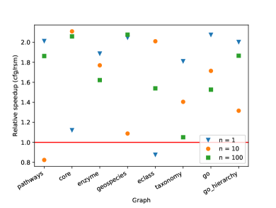
Figure 8. Multiple sources CFPQ reachability speedup (RSM over CFG) on RDF graphs and $G_{1}$

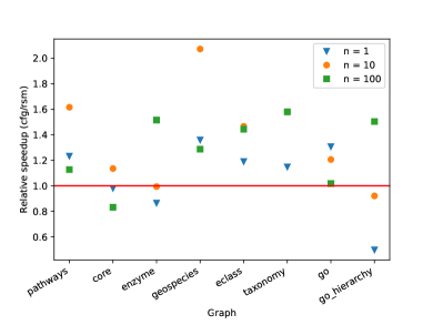
Figure 9. Multiple sources CFPQ reachability speedup (RSM over CFG) on RDF graphs and $G_{2}$

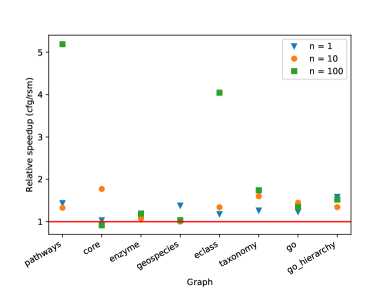
Figure 10. Multiple sources CFPQ reachability speedup (RSM over CFG) on RDF graphs and Geo

7. CFPQ For Neo4J

In this section we provide details on integration of GLL-based CFPQ to Neo4j graph database. We choose RSM-based version because our comparison (see section 6.1) shows that it is faster than BNF-based one.

Also, we provide results of implemented solution evaluation which shows that, first of all, provided solution faster then similar linear algebra based solution for RedisGraph. Also, we show that on RPQs our solution compatible with the Neo4j native one and in some cases evaluates queries successfully while native solution fails with OutOfMemory exception.

7.1. Implementation Details

Neo4j stored procedure is a mechanism through which query language can be extended by writing custom code in Java in such way that it can be called directly via Cypher.

We implemented Neo4j stored procedure which solves the reachability problem for the given set of start vertices and the given query. The procedure can be called as follows:

CALL cfpq.gll.getReachabilities(nodes, q)

where nodes is a collection of start nodes, and q is a string representation (or description) of RSM specified over relations types. Result of the given procedure is a stream of reachable pairs of nodes. Note that expressive power of our solution is limited: we can not use full power of Cypher inside our constraints. For example, we can not specify constrains on vertices inside our constraints.

We implemented a wrapper for Neo4j. Communication with the database is done using the Neo4j Native Java API. So, we used embedded database, which means it is run inside of the application and is not used as an external service.

Along with the existing modifications of GLL we made a Neo4j-specific one. Neo4j return result should be represented as a Stream and it is important to prevent early stream forcing, thus we changed all GLL internals to ensure that. This also has an added benefit that the query result is a stream, and thus it is possible to get the results on demand.

7.2. Evaluation

To assess the applicability of the proposed solution we evaluate it on a number of real-world graphs and queries. To estimate relative performance we compare our solution with matrix-based CFPQ algorithm implemented in RedisGraph by Arseniy Terekhov et al in (Terekhov et al., 2021). Also, we compare performance of evaluation of queries in reachability-only mode on regular path queries with native Neo4j solution.

The results of context-free path queries evaluation are presented in figures 11 for $G_{1}$, 12 for $G_{2}$, and 13 for Geo.

The results show that query evaluation time depends not only on a graph size or its sparsity, but also on an inner structure of the graph. For example, the relatively small graph go_hierarchy fully consists of edges used in queries $G_{1}$ and $G_{2}$, thus evaluation time for these queries is significantly bigger than for some bigger but more sparse graphs, for example, for eclass graph. Especially for relatively big start vertex set. Note, that the creation of relevant metrics for CFPQ queries evaluation time prediction is a challenging problem by itself and should be tackled in the future.

Also, we can see that in almost the all cases the proposed solution significantly faster than RedisGraph (in orders of magnitude in some cases). At the same time, in some cases (see results for graph core and all queries) RedisGraph outperforms our solution. Also, one can see, that evaluation time for RedisGraph is more predictable. For our solution in some cases execution time highly depends on start set. For example, see figure 13, graph enzyme.

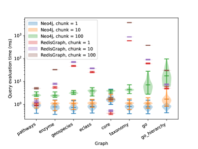
Figure 11. Multiple sources CFPQ reachability results for queries related to RDF analysis and $G_{1}$

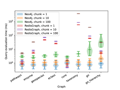
Figure 12. Multiple source CFPQ reachability results for queries related to RDF analysis and $G_{2}$

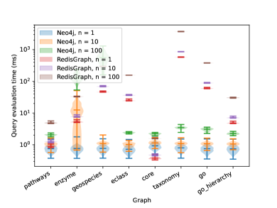
Figure 13. Multiple source CFPQ reachability results for queries related to RDF analysis and Geo

The particular important scenario is the case when the start set is a single vertex. The results of the single-source reachability show that such queries are reasonably fast: median time is about few milliseconds for all graphs and all queries. Note that even for single source queries, evaluation time highly depends on graph structure: evaluation time on core graph significantly bigger then for all other graphs for all queries. Note, that core is a smallest graph in terms of number of nodes and edges. Again, to provide an reliable metric to predict query execution time is a nontrivial task. Moreover, time grows with the size of a chunk, as expected.

Partial results for RPQ evaluation are presented in figures 14 and 15 for $\textit{reg}_{1}$ (defined in  13) and $\textit{reg}_{2}$ (defined in  14) respectively. For queries $\textit{reg}_{3}$ (defined in  15) and $\textit{reg}_{4}$ (defined in  16) we get similar results. Note, that on geospecies and taxonomy graphs native solution failed with OutOfMemory exception, while our solution evaluates queries successfully.

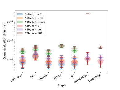
Figure 14. Multiple sources RPQ reachability results for queries related to RDF analysis and $\textit{reg}_{1}$ (native solution failed with OOM on last two graphs)

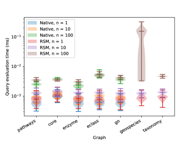
Figure 15. Multiple source RPQ reachability results for queries related to RDF analysis and $\textit{reg}_{2}$ (native solution failed with OOM on last two graphs)

We can see that the proposed solution slightly slower than native Neo4j algorithm, but not dramatically: typically less than two times. Moreover, in some cases our solution comparable with native one (see figure 14 and figure 15, graph eclass), and in some cases our solution faster than native one (see figure 15, graph core).

Finally, we conclude that not only the linear algebra based CFPQ algorithms can be used in real-world graph analysis systems: the proposed GLL-based solution outperforms linear algebra based one. Moreover, we show that the proposed solution can be used as a universal algorithm for both RPQ and CFPQ.

8. Related Work

The idea to use context-free grammars as constraints in path finding problem in graph databases was introduced and explored by Mihalis Yannakakis in (Yannakakis, 1990). A bit later, the same idea was developed by Thomas Reps et al. as a general framework for static code analysis (Reps et al., 1995). Further, this framework, called Context-Free Language Reachability (CFL-r), became one of the most popular and actively developed. The landscape analysis of the area was recently provided by Andreas Pavlogiannis in (Pavlogiannis, 2023). In the context of graph databases, the most recent systematic comparison of different CFPQ algorithms was done by Jochem Kuijpers et al. A set of CFPQ algorithms was implemented and evaluated using Neo4J as a graph storage. Results were presented in  (Kuijpers et al., 2019). It was concluded that the existing algorithms are not performant enough to be used for real-world data analysis.

Regarding graph databases, CFPQ was applied in such graph analysis related tasks as biological data analysis (Sevon and Eronen, 2008), data provenance (Miao and Deshpande, 2019), hierarchy analysis in RDF data (Medeiros et al., 2022; Zhang et al., 2016).

Multiple CFPQ algorithms are based on different parsing algorithms and techniques. For example, an approach based on parsing combinators was proposed by Ekaterina Verbitskaia et al. in (Verbitskaia et al., 2018). Several algorithms based on LL-like and LR-like techniques were developed by Ciro M. Medeiros et al. in (Medeiros et al., 2020, 2019, 2022). Also, CFPQ algorithms were investigated by Phillip Bradford in (Bradford and Thomas, 2009; Bradford, 2017) and Charles B. Ward et al. in (Ward et al., 2008). An algorithm based on matrix equations was proposed by Yuliya Susanina in (Susanina, 2020). Paths extraction problem was studied by Jelle Hellings in (Hellings, 2020).

A set of linear algebra-based CFPQ algorithms was developed, including all-paths and single-path versions, proposed by Rustam Azimov et al. in (Azimov et al., 2021) and (Terekhov et al., 2020) respectively, Kronecker product-based algorithm (Orachev et al., 2020) was proposed by Egor Orachev et al., and multiple-source CFPQ algorithm for RedisGraph was proposed by Arseniy Terekhov et al. in  (Terekhov et al., 2021).

Recursive state machines were studied in the context of CFPQ in several papers, including (Orachev et al., 2020) where Egor Orachev et al. use RSM to specify context-free constraints, Yuxiang Lei et al. (Lei et al., 2023) propose to use RSM to specify path constraints, and (Chaudhuri, 2008) where Swarat Chaudhuri proposes a slightly subcubic algorithm for reachability problem for recursive state machines — the equivalent to CFPQ problem.

GLL was introduced by Elizabeth Scott and Adrian Johnstone in (Scott and Johnstone, 2010). A number of modifications of the GLL algorithm were further proposed, including the version which supports EBNF without its transformation (Scott and Johnstone, 2018) and the version which uses binary subtree sets (Scott et al., 2019) instead of SPPF. The latest version simplifies the algorithm and avoids the overhead of explicit graph construction. Within it, the optimized and simplified OOP-friendly version of GLL was proposed by Ali Afroozeh and Anastasia Izmaylova in (Afroozeh and Izmaylova, 2015).

9. Conclusion and Future Work

In this work, we presented the GLL-based context-free path querying algorithm for Neo4j graph database. The implementation is available on GitHub: https://github.com/vadyushkins/cfpq-gll-neo4j-procedure.

Our solution uses Neo4j for graph storage, but the query language should be extended to support context-free constraints to make it useful. Both the extension of Cypher and the integration of our algorithm with the query engine are non-trivial challenges left for future work.

While GLL-based CFPQ potentially can be used to solve all-paths problem, currently we implemented the procedure for reachability problem only. Choosing useful strategies to enumerate paths and implementation of them is a direction for future research.

The most important direction for future work is to find a way to provide an incremental version of the GLL-based CFPQ algorithm to avoid full query reevaluation when the graph is only slightly changed. While our solution is based on the well-known parsing algorithm and there are solutions for incremental parsing, development of the efficient incremental version of the GLL-based CFPQ algorithm is a challenging problem left for future research.

Another direction is to create a parallel version of the GLL-based CFPQ algorithm to improve its performance on huge graphs. Although it seems natural to handle descriptors in parallel, the algorithm operates over global structures and the naive implementation of this idea leads to a significant overhead on synchronization.

- (1)
- Afroozeh and Izmaylova (2015) Ali Afroozeh and Anastasia Izmaylova. 2015. Faster, Practical GLL Parsing. In Compiler Construction, Björn Franke (Ed.). Springer Berlin Heidelberg, Berlin, Heidelberg, 89–108.
- Alur et al. (2005) Rajeev Alur, Michael Benedikt, Kousha Etessami, Patrice Godefroid, Thomas Reps, and Mihalis Yannakakis. 2005. Analysis of Recursive State Machines. ACM Trans. Program. Lang. Syst. 27, 4 (jul 2005), 786–818. https://doi.org/10.1145/1075382.1075387
- Azimov et al. (2021) Rustam Azimov, Ilya Epelbaum, and Semyon Grigorev. 2021. Context-Free Path Querying with All-Path Semantics by Matrix Multiplication. In Proceedings of the 4th ACM SIGMOD Joint International Workshop on Graph Data Management Experiences & Systems (GRADES) and Network Data Analytics (NDA) (Virtual Event, China) (GRADES-NDA ’21). Association for Computing Machinery, New York, NY, USA, Article 4, 7 pages. https://doi.org/10.1145/3461837.3464513
- Azimov and Grigorev (2018) Rustam Azimov and Semyon Grigorev. 2018. Context-free Path Querying by Matrix Multiplication. In Proceedings of the 1st ACM SIGMOD Joint International Workshop on Graph Data Management Experiences & Systems (GRADES) and Network Data Analytics (NDA) (Houston, Texas) (GRADES-NDA ’18). ACM, New York, NY, USA, Article 5, 10 pages. https://doi.org/10.1145/3210259.3210264
- Bar-Hillel et al. (1961) Y. Bar-Hillel, M. Perles, and E. Shamir. 1961. On formal properties of simple phrase structure grammars. Z. Phonetik Sprachwiss. Kommunikat. 14 (1961), 143–172.
- Bradford (2017) Phillip G. Bradford. 2017. Efficient exact paths for dyck and semi-dyck labeled path reachability (extended abstract). In 2017 IEEE 8th Annual Ubiquitous Computing, Electronics and Mobile Communication Conference (UEMCON). 247–253. https://doi.org/10.1109/UEMCON.2017.8249039
- Bradford and Thomas (2009) Phillip G. Bradford and David A. Thomas. 2009. Labeled shortest paths in digraphs with negative and positive edge weights. RAIRO - Theoretical Informatics and Applications 43, 3 (April 2009), 567–583. https://doi.org/10.1051/ita/2009011
- Chaudhuri (2008) Swarat Chaudhuri. 2008. Subcubic Algorithms for Recursive State Machines. In Proceedings of the 35th Annual ACM SIGPLAN-SIGACT Symposium on Principles of Programming Languages (San Francisco, California, USA) (POPL ’08). Association for Computing Machinery, New York, NY, USA, 159–169. https://doi.org/10.1145/1328438.1328460
- Grigorev and Ragozina (2017) Semyon Grigorev and Anastasiya Ragozina. 2017. Context-free Path Querying with Structural Representation of Result. In Proceedings of the 13th Central & Eastern European Software Engineering Conference in Russia (St. Petersburg, Russia) (CEE-SECR ’17). ACM, New York, NY, USA, Article 10, 7 pages. https://doi.org/10.1145/3166094.3166104
- Hellings (2014) Jelle Hellings. 2014. Conjunctive context-free path queries. In Proceedings of ICDT’14. 119–130.
- Hellings (2020) Jelle Hellings. 2020. Explaining Results of Path Queries on Graphs. In Software Foundations for Data Interoperability and Large Scale Graph Data Analytics, Lu Qin, Wenjie Zhang, Ying Zhang, You Peng, Hiroyuki Kato, Wei Wang, and Chuan Xiao (Eds.). Springer International Publishing, Cham, 84–98.
- Kuijpers et al. (2019) Jochem Kuijpers, George Fletcher, Nikolay Yakovets, and Tobias Lindaaker. 2019. An Experimental Study of Context-Free Path Query Evaluation Methods. In Proceedings of the 31st International Conference on Scientific and Statistical Database Management (Santa Cruz, CA, USA) (SSDBM ’19). ACM, New York, NY, USA, 121–132. https://doi.org/10.1145/3335783.3335791
- Lei et al. (2023) Yuxiang Lei, Yulei Sui, Shin Hwei Tan, and Qirun Zhang. 2023. Recursive State Machine Guided Graph Folding for Context-Free Language Reachability. Proc. ACM Program. Lang. 7, PLDI, Article 119 (jun 2023), 25 pages. https://doi.org/10.1145/3591233
- Medeiros et al. (2018) Ciro M. Medeiros, Martin A. Musicante, and Umberto S. Costa. 2018. Efficient Evaluation of Context-Free Path Queries for Graph Databases. In Proceedings of the 33rd Annual ACM Symposium on Applied Computing (Pau, France) (SAC ’18). Association for Computing Machinery, New York, NY, USA, 1230–1237. https://doi.org/10.1145/3167132.3167265
- Medeiros et al. (2019) Ciro M. Medeiros, Martin A. Musicante, and Umberto S. Costa. 2019. LL-based query answering over RDF databases. Journal of Computer Languages 51 (2019), 75–87. https://doi.org/10.1016/j.cola.2019.02.002
- Medeiros et al. (2020) Ciro M. Medeiros, Martin A. Musicante, and Umberto S. Costa. 2020. An Algorithm for Context-Free Path Queries over Graph Databases. In Proceedings of the 24th Brazilian Symposium on Context-Oriented Programming and Advanced Modularity (Natal, Brazil) (SBLP ’20). Association for Computing Machinery, New York, NY, USA, 40–47. https://doi.org/10.1145/3427081.3427087
- Medeiros et al. (2022) Ciro M. Medeiros, Martin A. Musicante, and Umberto S. Costa. 2022. Querying graph databases using context-free grammars. Journal of Computer Languages 68 (2022), 101089. https://doi.org/10.1016/j.cola.2021.101089
- Miao and Deshpande (2019) H. Miao and A. Deshpande. 2019. Understanding Data Science Lifecycle Provenance via Graph Segmentation and Summarization. In 2019 IEEE 35th International Conference on Data Engineering (ICDE). 1710–1713.
- Orachev et al. (2020) Egor Orachev, Ilya Epelbaum, Rustam Azimov, and Semyon Grigorev. 2020. Context-Free Path Querying by Kronecker Product. In Advances in Databases and Information Systems, Jérôme Darmont, Boris Novikov, and Robert Wrembel (Eds.). Springer International Publishing, Cham, 49–59.
- Pacaci et al. (2020) Anil Pacaci, Angela Bonifati, and M. Tamer Özsu. 2020. Regular Path Query Evaluation on Streaming Graphs. In Proceedings of the 2020 ACM SIGMOD International Conference on Management of Data (Portland, OR, USA) (SIGMOD ’20). Association for Computing Machinery, New York, NY, USA, 1415–1430. https://doi.org/10.1145/3318464.3389733
- Pavlogiannis (2023) Andreas Pavlogiannis. 2023. CFL/Dyck Reachability: An Algorithmic Perspective. ACM SIGLOG News 9, 4 (feb 2023), 5–25. https://doi.org/10.1145/3583660.3583664
- Rehof and Fähndrich (2001) Jakob Rehof and Manuel Fähndrich. 2001. Type-Base Flow Analysis: From Polymorphic Subtyping to CFL-Reachability. SIGPLAN Not. 36, 3 (Jan. 2001), 54–66. https://doi.org/10.1145/373243.360208
- Rekers (1992) Jan G Rekers. 1992. Parser generation for interactive environments. Ph. D. Dissertation. Citeseer.
- Reps et al. (1995) Thomas Reps, Susan Horwitz, and Mooly Sagiv. 1995. Precise Interprocedural Dataflow Analysis via Graph Reachability. In Proceedings of the 22nd ACM SIGPLAN-SIGACT Symposium on Principles of Programming Languages (San Francisco, California, USA) (POPL ’95). Association for Computing Machinery, New York, NY, USA, 49–61. https://doi.org/10.1145/199448.199462
- Rodriguez-Prieto et al. (2020) Oscar Rodriguez-Prieto, Alan Mycroft, and Francisco Ortin. 2020. An Efficient and Scalable Platform for Java Source Code Analysis Using Overlaid Graph Representations. IEEE Access 8 (2020), 72239–72260. https://doi.org/10.1109/ACCESS.2020.2987631
- Santos et al. (2018) Fred C. Santos, Umberto S. Costa, and Martin A. Musicante. 2018. A Bottom-Up Algorithm for Answering Context-Free Path Queries in Graph Databases. In Web Engineering, Tommi Mikkonen, Ralf Klamma, and Juan Hernández (Eds.). Springer International Publishing, Cham, 225–233.
- Scott and Johnstone (2010) Elizabeth Scott and Adrian Johnstone. 2010. GLL Parsing. Electronic Notes in Theoretical Computer Science 253, 7 (2010), 177–189. https://doi.org/10.1016/j.entcs.2010.08.041 Proceedings of the Ninth Workshop on Language Descriptions Tools and Applications (LDTA 2009).
- Scott and Johnstone (2013) Elizabeth Scott and Adrian Johnstone. 2013. GLL parse-tree generation. Science of Computer Programming 78, 10 (2013), 1828–1844. https://doi.org/10.1016/j.scico.2012.03.005 Special section on Language Descriptions Tools and Applications (LDTA’08 & ’09) & Special section on Software Engineering Aspects of Ubiquitous Computing and Ambient Intelligence (UCAmI 2011).
- Scott and Johnstone (2018) Elizabeth Scott and Adrian Johnstone. 2018. GLL syntax analysers for EBNF grammars. Science of Computer Programming 166 (2018), 120–145. https://doi.org/10.1016/j.scico.2018.06.001
- Scott et al. (2019) Elizabeth Scott, Adrian Johnstone, and L. Thomas van Binsbergen. 2019. Derivation representation using binary subtree sets. Science of Computer Programming 175 (2019), 63–84. https://doi.org/10.1016/j.scico.2019.01.008
- Sevon and Eronen (2008) Petteri Sevon and Lauri Eronen. 2008. Subgraph Queries by Context-free Grammars. Journal of Integrative Bioinformatics 5, 2 (2008), 157 – 172. https://doi.org/10.1515/jib-2008-100
- Susanina (2020) Yuliya Susanina. 2020. Context-Free Path Querying via Matrix Equations. In Proceedings of the 2020 ACM SIGMOD International Conference on Management of Data (Portland, OR, USA) (SIGMOD ’20). Association for Computing Machinery, New York, NY, USA, 2821–2823. https://doi.org/10.1145/3318464.3384400
- Terekhov et al. (2020) Arseniy Terekhov, Artyom Khoroshev, Rustam Azimov, and Semyon Grigorev. 2020. Context-Free Path Querying with Single-Path Semantics by Matrix Multiplication. In Proceedings of the 3rd Joint International Workshop on Graph Data Management Experiences & Systems (GRADES) and Network Data Analytics (NDA) (Portland, OR, USA) (GRADES-NDA’20). Association for Computing Machinery, New York, NY, USA, Article 5, 12 pages. https://doi.org/10.1145/3398682.3399163
- Terekhov et al. (2021) Arseniy Terekhov, Vlada Pogozhelskaya, Vadim Abzalov, Timur Zinnatulin, and Semyon V. Grigorev. 2021. Multiple-Source Context-Free Path Querying in Terms of Linear Algebra. In Proceedings of the 24th International Conference on Extending Database Technology, EDBT 2021, Nicosia, Cyprus, March 23 - 26, 2021, Yannis Velegrakis, Demetris Zeinalipour-Yazti, Panos K. Chrysanthis, and Francesco Guerra (Eds.). OpenProceedings.org, 487–492. https://doi.org/10.5441/002/edbt.2021.56
- Verbitskaia et al. (2018) Ekaterina Verbitskaia, Ilya Kirillov, Ilya Nozkin, and Semyon Grigorev. 2018. Parser Combinators for Context-Free Path Querying. In Proceedings of the 9th ACM SIGPLAN International Symposium on Scala (St. Louis, MO, USA) (Scala 2018). Association for Computing Machinery, New York, NY, USA, 13–23. https://doi.org/10.1145/3241653.3241655
- Wang et al. (2019) Xin Wang, Simiao Wang, Yueqi Xin, Yajun Yang, Jianxin Li, and Xiaofei Wang. 2019. Distributed Pregel-based provenance-aware regular path query processing on RDF knowledge graphs. World Wide Web 23, 3 (Nov. 2019), 1465–1496. https://doi.org/10.1007/s11280-019-00739-0
- Ward et al. (2008) Charles B. Ward, Nathan M. Wiegand, and Phillip G. Bradford. 2008. A Distributed Context-Free Language Constrained Shortest Path Algorithm. In 2008 37th International Conference on Parallel Processing. 373–380. https://doi.org/10.1109/ICPP.2008.67
- Yannakakis (1990) Mihalis Yannakakis. 1990. Graph-Theoretic Methods in Database Theory. In Proceedings of the Ninth ACM SIGACT-SIGMOD-SIGART Symposium on Principles of Database Systems (Nashville, Tennessee, USA) (PODS ’90). Association for Computing Machinery, New York, NY, USA, 230–242. https://doi.org/10.1145/298514.298576
- Zhang et al. (2016) Xiaowang Zhang, Zhiyong Feng, Xin Wang, Guozheng Rao, and Wenrui Wu. 2016. Context-Free Path Queries on RDF Graphs. In The Semantic Web – ISWC 2016, Paul Groth, Elena Simperl, Alasdair Gray, Marta Sabou, Markus Krötzsch, Freddy Lecue, Fabian Flöck, and Yolanda Gil (Eds.). Springer International Publishing, Cham, 632–648.
- Zheng and Rugina (2008) Xin Zheng and Radu Rugina. 2008. Demand-driven Alias Analysis for C. In Proceedings of the 35th Annual ACM SIGPLAN-SIGACT Symposium on Principles of Programming Languages (San Francisco, California, USA) (POPL ’08). ACM, New York, NY, USA, 197–208. https://doi.org/10.1145/1328438.1328464