Learning flow functions of spiking systems

Abstract

We propose a framework for surrogate modelling of spiking systems. These systems are often described by stiff differential equations with high-amplitude oscillations and multi-timescale dynamics, making surrogate models an attractive tool for system design and simulation. We parameterise the flow function of a spiking system using a recurrent neural network architecture, allowing for a direct continuous-time representation of the state trajectories. The spiking nature of the signals makes for a data-heavy and computationally hard training process; thus, we describe two methods to mitigate these difficulties. We demonstrate our framework on two conductance-based models of biological neurons, showing that we are able to train surrogate models which accurately replicate the spiking behaviour.

1 Introduction

We consider the problem of learning surrogate models of spiking systems from samples of state trajectories. Spiking behaviours abound in dynamical system models of biological neurons, and there is significant interest in reproducing such behaviour in electronic devices. We propose a data-driven framework based on a recurrent neural network (RNN) architecture to approximate the flow function of conductance-based state-space models of spiking systems in continuous time.

Spiking systems (Sepulchre, 2022) are dynamical systems whose stability behaviour is highly input-dependent. Determined by the input excitation, the state typically either remains close to an equilibrium or enters into a limit cycle with large-amplitude oscillations called spikes. Whether the input excites the system into the oscillatory regime and how many spikes are emitted depends on both the input amplitude and frequency (Sepulchre et al., 2018). These systems thus possess a mixed continuous–discrete character, as the spikes can be seen as encoding digital information into a continuous-time signal. Models of biological neurons provide prototypical examples of spiking systems, where the input is a current and the spiking phenomenon is observed in the membrane potential.

Significant effort in computational neuroscience has been devoted to modelling the spiking behaviour of neurons. Hodgkin and Huxley (1952) proposed modelling the relationship between the membrane voltage and the applied current as a parallel interconnection of nonlinear conductances, which can be identified using a voltage-clamp experiment, which Burghi et al. (2021) relate to a general output feedback system identification scheme. The parameter identification problem is shown to be tractable thanks to stability properties of the inverse dynamics of the conductance-based models.

Circuit-theoretic models of biological neurons suggest the possibility of building electronic devices with spiking behaviour, conceivably combining the best features of analogue and digital electronics in a single physical device (Mead, 1990; DeWeerth et al., 1991; Sepulchre, 2022). Using these biologically-inspired components in circuit design requires the ability to efficiently simulate their behaviour, possibly in interconnection with many other circuit elements. However, the differential equations models of these systems are typically stiff, which suggests that surrogate models may provide computational advantages over direct integration of the differential equations. Furthermore, continuous-time representations are desirable, due to the possibly input-dependent nature of the periodicity of the spike trains, the high-frequency nature of the spike signals, and the multiple time scales involved in the dynamics.

Machine learning offers an attractive array of methods for constructing surrogate models of dynamical systems. Focusing on continuous-time models, we can distinguish between two approaches in the literature: those methods that attempt to learn a model of the system dynamics from data, and those where the goal is to directly learn a solution operator associated to the system. In the first class of methods, a neural network is typically used to parameterise the right-hand side of an ordinary differential equation (ODE), resulting in a class of models known as neural ODEs. This requires a way to automatically compute gradients of trajectory values with respect to network parameters during training, which may be done by differentiating through an ODE solver or using an adjoint method (Chen et al., 2018). In a surrogate modelling context, Yang et al. (2022) propose a neural ODE method for learning models of complex circuit elements, and derive a parameterisation of the network that guarantees input-to-state stability. Regarding the application of these models in system identification, Forgione and Piga (2021) discuss model structures and fitting criteria, and Beintema et al. (2023) propose an architecture and estimation method shown to compete with state-of-the-art nonlinear identification methods. The second group of methods, broadly known as operator learning, attempt instead to directly learn the solution map of a differential equation, i.e., the mapping from initial conditions, parameters, and external inputs to the solution. Directly parameterising the solution allows for fast evaluation for new inputs, and provided that standard deep learning toolchains are used, gradients with respect to the inputs of the model also become easy to compute. A great deal of research attention has focused on learning solution operators of partial differential equations using integral kernel parameterisations composed with neural networks (Lu et al., 2021; Li et al., 2021; Kissas et al., 2022). Lin et al. (2023) use one such parameterisation in a recursive architecture to predict trajectories of dynamical systems with external inputs. In a similar context, Qin et al. (2021) suggest a residual network-based architecture to approximate the one-step-ahead map of a dynamical system. Biloš et al. (2021) suggest a number of architectures inspired by flow functions of autonomous systems as a substitute for neural ODEs.

Our main contribution is an operator learning framework for constructing continuous-time input–output surrogate models of spiking systems from samples of state trajectories. Starting from the flow function description of the spiking system, we directly parameterise its state trajectories. This is particularly suited for systems exhibiting spiking behaviour, as it allows for a continuous-time description of the state trajectories, while not requiring sampling the derivatives of the states (which due to the spikes can widely vary in amplitude). Indeed, from the flow function point of view the problem can be formulated as a standard (albeit infinite-dimensional) regression problem. Furthermore, by imposing the non-restrictive assumption that the input signal is piecewise constant, we show that there is an exact correspondence between the flow function and a discrete-time dynamical system. This suggests that one can approximate the flow function by an RNN, resulting in an architecture that uses only standard learning components and can be easily implemented and trained with established deep learning toolchains. Due to the nature of the spike signals, the trajectories must be densely sampled in order to correctly capture the timing and height of each spike. We propose a simple data reduction method based on rejection sampling, which enables a significant reduction of the required amount of time samples per trajectory by focusing on the most important regions of the signal. This is made possible by our continuous-time approach, which naturally allows for data that is irregularly sampled in time. Moreover, we show how the complexity of the optimisation problem can be subdued by considering segments of trajectories, using the properties of the flow function. We numerically evaluate the our approach through simulations of conductance-based models of a single neuron and an interconnection of two neurons. We build upon our recent work (Aguiar et al., 2023a) in which we describe a neural network architecture for learning flow functions of continuous-time control systems. In the current paper, we focus explicitly on challenges arising in learning the dynamics of spiking systems which require special attention when applying this architecture.

The remainder of the paper is organised as follows. In section 2 we introduce conductance-based neuron models in state-space form as a prototype for spiking behaviours, define the concept of flow function of a control system, and formulate the problem of constructing a surrogate model of such a system as an optimisation problem. In section 3 we describe the proposed architecture and two methods for reducing the complexity of the training process. Finally, in section 4 we report and discuss results from numerical experiments, and in section 5 we conclude and discuss possibilities for future work.

2 Problem formulation

We begin by introducing a class of state-space models of biological neurons and their interconnections which serve as prototypical examples of systems exhibiting spiking behaviour, before introducing the definition of the flow function of a control system and the mathematical formulation of the surrogate modelling problem for these systems.

2.1 Conductance-based models

The general conductance-based model of a neuron is given by the system of differential equations (Burghi et al., 2021)

$$\aligned C_{m}\dot{V}(t)&=u(t)-g_{\text{leak}}(V(t)-V_{\text{leak}})-\sum_{k=1}^{N_{I}}I_{k}(V(t),m_{k},n_{k})\\ \dot{m}(t)=A_{m}(V(t))m(t)+b_{m}(V(t))\\ \dot{n}(t)=A_{n}(V(t))n(t)+b_{n}(V(t)),$$ (1)

where $V$ is the membrane potential, $u$ the external (input) current, $C_{m}>0$ the membrane capacitance, $g_{\text{leak}}$ a leak conductance, and $V_{\text{leak}}$ the reversal potential. The gating variables $m,n\in[0,1]^{N_{I}}$ are dimensionless, and $A_{m}(V),A_{n}(V)$ are diagonal matrices depending on $V$. The ionic currents are given by $I_{k}(V,m_{k},n_{k})=g_{k}m_{k}^{\alpha_{k}}n_{k}^{\beta_{k}}(V-V_{k})$, where $g_{k}>0$ and $V_{k}\in{\mathbb{R}}$ are constants and $\alpha_{k},\beta_{k}$ are nonnegative integers. A detailed description of this class of models and their biological motivation is given in Hodgkin and Huxley (1952) and Pospischil et al. (2008). These models are prototypes of spiking systems: for certain choices of the input current one observes spiking behaviour in the membrane potential signal $V$ (Sepulchre et al., 2018).

One can interconnect several neuron models eq:cond-model to obtain more complex spiking behaviours (Giannari and Astolfi, 2022). In particular, we can model the interconnection of $n$ neurons through electrical synapses

$$C^{i}_{m}\dot{V}_{i}(t)=u_{i}(t)-g^{i}_{\text{leak}}(V_{i}(t)-V^{i}_{\text{leak}})-\sum_{k=1}^{N^{i}_{I}}I^{i}_{k}(V_{i}(t),m^{i}_{k},n^{i}_{k})+\sum_{j=1}^{n}{\epsilon_{ij}(V_{j}(t)-V_{i}(t))},$$ (2)

where $m^{i}$ and $n^{i}$ satisfy differential equations with the same structure as those in eq:cond-model (depending only on $V_{i}$).

2.2 Flow functions

Consider a dynamical system described in state-space form by

$$\aligned\dot{\xi}(t)&=f(\xi(t),u(t)),~{}\xi(0)=x\\ \eta(t)=h(\xi(t)),$$ (3)

with state $\xi(t)\in{\mathbb{R}}^{d_{x}}$, input $u(t)\in{\mathbb{R}}^{d_{u}}$ and output $\eta(t)\in{\mathbb{R}}^{d_{y}}$. Assume that $f$ is such that solutions to eq:ode exist on ${\mathbb{R}}_{\geq 0}$ for $x\in{\mathcal{X}}$, with ${\mathcal{X}}\subset{\mathbb{R}}^{d_{x}}$ being an invariant set, and $u:{\mathbb{R}}_{\geq 0}\to{\mathcal{U}}$ is measurable and essentially bounded. Define a map ${{\varphi}:{\mathbb{R}}_{\geq 0}\times{\mathcal{X}}\times{\mathbb{U}}\to{\mathcal{X}}}$, ${\mathbb{U}}:=L^{\infty}({\mathbb{R}}_{\geq 0},{\mathcal{U}})$, such that for any such $x$ and $u$ it holds that $\xi(t)={\varphi}(t,x,u),~{}t\geq 0$. The map ${\varphi}$ is called the flow function of eq:ode. The flow function satisfies the identity property: for any $\xi\in{\mathcal{X}}$ and $u\in{\mathbb{U}}$, ${\varphi}(0,x,u)=x$; and the semigroup property: for any $x\in{\mathcal{X}}$, $t,s\geq 0$ and $u,v\in{\mathbb{U}}$, ${\varphi}(t+s,x,u\underset{{s}}{\wedge}v)={\varphi}(t,{\varphi}(s,x,u),v)$. Here $u\underset{{s}}{\wedge}v$ denotes the concatenation of $u$ and $v$ at time $s\geq 0$, defined as $[{u\underset{{s}}{\wedge}v}]{(t)}=u(t)$, $0\leq t<s$, and $[{u\underset{{s}}{\wedge}v}]{(t)}=v(t-s)$, $t\geq s$.

Henceforth we assume that the considered controls are piecewise constant with sampling period $\Delta>0$. Thus, let ${\mathbb{U}}_{\Delta}\subset{\mathbb{U}}$, where $\Delta>0$ and $u\in{\mathbb{U}}_{\Delta}$ if and only if there exists a sequence ${(\omega_{k})_{k=0}^{\infty}\subset{\mathcal{U}}}$ such that $u(k\Delta+t)=\omega_{k},~{}k\geq 1,~{}t\in[0,\Delta)$. We restrict ${\varphi}$ to $\bigcup_{s\geq 0}\sigma^{s}({\mathbb{U}}_{\Delta})$, where $\sigma$ is the time-shift operator defined by $(\sigma^{s}u)(t)=u(t+s)$ for $s\geq 0$.

The conductance-based models eq:cond-model and eq:cond-model-multi can be written in the form eq:ode, with the state $\xi$ given by the membrane potentials $V_{i}$ together with the gating variables $m^{i}_{k},n^{i}_{k}$ of each neuron and the input signal $u$ given by the collection of input currents $u_{i}$. We take the output $\eta$ to be the collection of membrane potentials $V_{i}$, as these are the spiking signals we are interested in simulating and, as in eq:cond-model-multi, the relevant signals when interconnecting neuron models.

2.3 Problem

Let us now define the problem considered in this paper. Let $y(t,x,u):=h({\varphi}(t,x,u))$ be the trajectory of the output signal. We define the problem of obtaining a surrogate model of the system eq:ode as that of solving the optimisation problem

$$\underset{\hat{y}\in{\mathcal{H}}}{\text{minimise}}~{}~{}\ell_{T}(\hat{y}):={\mathbf{E}}_{x,u}~{}\frac{1}{T}\int_{0}^{T}{\left\|{y(t,x,u)-\hat{y}(t,x,u)}\right\|_{1}\mathrm{d}{t}},$$ (4)

where $x,u$ are assumed to be independent and distributed according to probability distributions $P_{x}$ and $P_{u}$, describing the initial conditions and control inputs of interest, respectively. The distribution $P_{u}$ has its range in ${\mathbb{U}}_{\Delta}$, so that sampling the values of a control $u\sim P_{u}$ on $[0,T]$ is equivalent to sampling a finite sequence of control values. We use the $1$-norm to measure the approximation error due to the sparse nature of the spike signals. The set ${\mathcal{H}}$ is the hypothesis class from which the surrogate model $\hat{y}$ is to be selected. In this paper, we consider an hypothesis class given by the RNN architecture described in the following section.

3 Methodology

In this section, we first motivate the approximation of the flow function by an RNN and describe the proposed architecture. We then discuss the data collection process and two issues arising in the training of the RNN architecture, as well as methods to mitigate them.

3.1 Architecture

Fix $t\geq 0$, $x\in{\mathcal{X}}$ and $u\in{\mathbb{U}}_{\Delta}$. Let $(\omega_{k})$ be the sequence of values of $u$, and define for $\omega\in{\mathcal{U}}$ the constant control $u_{\omega}$ through $u_{\omega}(t):=\omega$. With $k_{t}:=\lfloor t/\Delta\rfloor$, the value of ${\varphi}(t,x,u)$ can be evaluated recursively as follows:

$$\aligned x_{0}&=x\\ x_{k+1}={\varphi}(\Delta,x_{k},u_{\omega_{k}}),~{}0\leq k<k_{t}\\ x_{k_{t}+1}={\varphi}(t-k_{t}\Delta,x_{k_{t}},u_{\omega_{k_{t}}}).$$ (5)

By the semigroup property, we then have $x_{k_{t}+1}={\varphi}(t,x,u)$. Letting $\Phi:[0,1]\times{\mathcal{X}}\times{\mathcal{U}}\to{\mathcal{X}}$ be defined by $\Phi(\tau,x,\omega)={\varphi}(\tau\Delta,x,u_{\omega})$, and $\tau_{k},k=0,\dots,k_{t}$ by $\tau_{k}=1,\ k<k_{t}$ and ${\tau_{k_{t}}=(t-k_{t}\Delta)/\Delta}$, we can rewrite eq:flow-recurrence as $x_{k+1}=\Phi(\tau_{k},x_{k},{\omega_{k}})$, $0\leq k\leq k_{t}$. If now $v\in\bigcup_{s\geq 0}\sigma^{s}({\mathbb{U}}_{\Delta})$, there is some $u\in{\mathbb{U}}_{\Delta}$ and $\delta\in[0,\Delta)$ such that $v=\sigma^{\delta}u$, and by the semigroup property ${\varphi}(t,x,v)={\varphi}(t-\delta,{\varphi}(\delta,x,u_{\omega_{0}}),\sigma^{\Delta}u)$ for $t\geq\delta$. Thus, since $\sigma^{\Delta},u_{\omega_{0}}\in{\mathbb{U}}_{\Delta}$, one can proceed as above also in this case. This shows that the flow can be exactly computed at any time instant by a discrete-time finite-dimensional dynamical system (with inputs $(\tau,\omega)$), suggesting that one can approximate ${\varphi}$ (and thus $y$) through this representation.

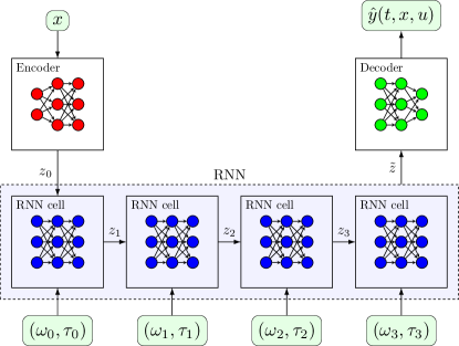
Figure 1: Schematic of the proposed architecture for $k_{t}=3$.

The previous derivation motivates the choice of the hypothesis class ${\mathcal{H}}$ given by a parameterisation of $\hat{y}$ based on the composition of an RNN with a pair of encoder–decoder networks, as illustrated in Figure 1. This architecture is in fact a universal approximator of the flow function corresponding to eq:ode under mild conditions on $f$ (Aguiar et al., 2023b).

3.2 Data collection

To generate training data, we integrate the differential equation eq:ode with $x$ and $u$ sampled from $P_{x}$ and $P_{u}$, respectively, obtaining samples

$$\xi_{ik}={\varphi}(t_{ik},x_{i},u_{i}),~{}k=1,\dots,K,~{}i=1,\dots,N,$$ (6)

where $t_{ik}$ are sampled uniformly on $[0,T]$. Using these samples, we construct an approximation of $\ell_{T}$ in eq:loss as

$$\hat{\ell}_{T}(\hat{y}):=\frac{1}{N}\frac{1}{K}\sum_{i,k}\left\|{h(\xi_{ik})-\hat{y}(t_{ik},x_{i},u_{i})}\right\|_{1}.$$ (7)

Because ${\varphi}$ is the flow of a spiking system, the optimisation of eq:emp-loss is not without challenges. The spikes can be very ‘thin’, which can imply that a large number of samples are required when the sampling times $t_{ik}$ are uniformly distributed, increasing the computational load during training. Furthermore, the spikes might be relatively infrequent, and consequently underrepresented in the data, which can make it harder to learn the spiking behaviour properly. In the next subsection we describe a simple rejection sampling algorithm that alleviates these issues.

3.3 Rejection sampling for data reduction

We propose a method that simultaneously reduces the amount of samples per trajectory needed to represent the spike signal and weights the loss function in order to emphasise learning the spiking behaviour. This is done as follows: first, sample data eq:samples with $t_{ik}$ uniform and dense, and then use rejection sampling to ‘prune’ the data, i.e., select which samples to remove so that the remaining $t_{ik}$ have a distribution which favours learning the spiking behaviour correctly.

Consider first the case of a single output, i.e., $y$ is scalar-valued. Roughly speaking, the output signal $y(\cdot,x,u)$ has higher frequency content when its amplitude is higher (i.e., when a spike is emitted). One should thus sample more densely when the value of $y(\cdot,x,u)$ is higher. In other words, we would like that the sampling times $t_{ik}$ be distributed according to the density function $p(t,x_{i},u_{i})\propto\left[{y(t,x_{i},u_{i})-\min_{s\in[0,T]}{y(s,x_{i},u_{i})}}\right]$ (or $p\propto\alpha(y)$, where $\alpha$ is an increasing function). If $t_{ik}$ are sampled with this density, $\hat{\ell}_{T}$ in eq:emp-loss is the empirical estimate of the weighted loss function

$${\mathbf{E}}_{x,u}~{}\frac{1}{T}\int_{0}^{T}{p(t,x,u)\left\|{y(t,x,u)-\hat{y}(t,x,u)}\right\|_{1}\mathrm{d}{t}},$$

giving higher weight to parts of the trajectories where spiking occurs.

In our case, where $t_{ik}$ are given a priori and uniformly distributed, we can use rejection sampling (Ross, 2013) to discard certain samples so that the remaining $t_{ik}$ are distributed approximately according to $p$. This implies the following procedure for each time sample $t_{ik}$:

• Draw $\Upsilon_{ik}\sim{\text{Uniform}{\left({[0,1]}\right)}}$;

• If $\Upsilon_{ik}>\frac{Tp(t_{ik},x_{i},u_{i})}{M_{i}}$, where $M_{i}:=\max_{k}Tp(t_{ik},x_{i},u_{i})$, remove the sample.

After a single pass through the dataset, the undiscarded $t_{ik}$ will be approximately distributed with density $p(\cdot,x_{i},u_{i})$. Furthermore, the probability of accepting a sample from the $i$th trajectory is approximately equal to $1/M_{i}$, giving the approximate fraction of samples which will be retained.

We are thus at once able to reduce the volume of data while retaining a faithful representation of the spiking signals, and to increase the weight of the spiking regions in the loss function. Other choices of $p$, e.g., involving the derivative or frequency content of the output signal, could of course also be used.

If there are several outputs, so $y$ is vector-valued, one may combine the outputs into a scalar signal that contains the spikes of all outputs, for instance, $p(t,x,u)\propto\max_{i=1,\dots,d_{y}}\alpha_{i}(y_{i}(t,x,u))$, where $\alpha_{i}$ are monotone functions to ensure that $y_{i}$, $i=1,\dots,d_{y}$, are normalised to the same range.

3.4 Windowed loss using the semigroup property

The complexity of optimising the empirical loss eq:emp-loss with an RNN is highly dependent on the length of the input sequences. This dependence is twofold: the computational effort of the forward and backward passes through the recurrent network depends linearly on the simulation length, while simultaneously the loss function becomes less smooth with respect to the network parameters as the sequence length increases (Ribeiro et al., 2020). We describe here how this issue can be addressed in the context of our method, by reducing the length of input sequences while still making use of all training data. In a similar way to Ribeiro et al. (2020) and Beintema et al. (2023), we construct a new loss function by considering shorter segments of output trajectories. This is easy to do in our setting, as we can take advantage of properties of the flow function.

It follows from the semigroup property that for $j\geq k$ we have $\xi_{ij}={\varphi}(t_{ij}-t_{ik},\xi_{ik},\sigma^{t_{ik}}u_{i})$. Hence, with the same training data we can construct the loss function

$$\hat{\ell}^{\text{win}}(\hat{y}):=\frac{1}{N}\frac{1}{K}\sum_{i,k}\frac{1}{\left|{J_{ik}}\right|}\sum_{j\in J_{ik}}{\left\|{h(\xi_{ij})-\hat{y}(t_{ij}-t_{ik},\xi_{ik},\sigma^{t_{ik}}u_{i})}\right\|_{1}},$$

where $J_{ik}$ are sets of indices such that $j\geq k$ for all $j\in J_{ik}$, and $\left|{J_{ik}}\right|$ denotes the cardinality of $J_{ik}$. In this case, the maximum length of the input sequences is given by ${L:=1+\max_{i,k}\max_{j\in J_{ik}}\lfloor{\frac{t_{ij}-t_{ik}}{\Delta}}\rfloor}$, which we can choose by appropriate selection of the index sets $J_{ik}$. This allows for controlling the time complexity of the training epochs and the smoothness of the loss function. Of course, it is not necessarily the case that $\hat{\ell}^{\text{win}}$ is the empirical mean approximation of $\ell_{T}$, so care must be taken to avoid overfitting.

4 Numerical experiments

We perform two experiments with data from simulations of two conductance-based models: a single neuron model, and a model of the feedforward interconnection of two neurons with an electrical synapse.

4.1 Model of a single fast-spiking neuron

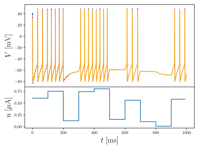
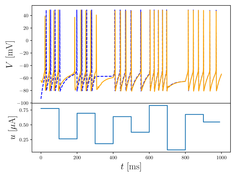
Figure 2: Predictions of output trajectories for a single fast-spiking neuron. The surrogate model prediction is shown in orange; the real output is plotted in blue (dashed). Note that the surrogate model closely reproduces the spiking behaviour of the neuron model, and is able recover from errors in the prediction of the initial condition.

Dynamics

We consider a conductance-based model of a single neuron as in eq:cond-model with a sodium current, $I_{1}(V,m_{1},n_{1})=g_{1}m_{1}^{3}n_{1}(V-V_{1})$, and a potassium ionic current, $I_{2}(V,m_{2},n_{2})=g_{2}n_{2}^{4}(V-V_{2})$, i.e., $N_{I}=2$. The model can be described with four states, since ${\alpha_{2}=0}$ and so $m_{2}$ can be ignored. This corresponds to a fast-spiking neuron, and is identical to the model structure originally proposed in Hodgkin and Huxley (1952). The full equations and parameter values may be found in Giannari and Astolfi (2022).

Data collection

We integrate $N=800$ state trajectories of the model over $t\in[0,T]$, ${T=500}$ ms, using a backwards differentiation formula integrator, and collect $K=50000$ samples from each trajectory, with $t_{ik}$ sampled uniformly using Latin hypercube sampling. The initial conditions are sampled uniformly with ${V(0)\sim{\text{Uniform}{\left({[-100,100]}\right)}}}$ mV and ${m_{k}(0),n_{k}(0)\sim{\text{Uniform}{\left({[0,1]}\right)}}}$. The control inputs have period ${\Delta=10}$ ms and input values are sampled according to

$$\aligned\omega_{10k}&\overset{\text{i.i.d.}}{\sim}{\text{Uniform}{\left({[0,1]}\right)}}~{}\mu\text{A},\ k\geq 0\\ \omega_{10k+j}=\omega_{10k},\ k\geq 0,\ 0\leq j<10,$$

i.e. the input changes every 100 ms.

We reduce the dataset using the rejection sampling method described above, sampling according to the density $p(t,x,u)\propto\tilde{y}(t,x,u)$, where $\tilde{y}$ is the normalisation of the output $y$ to $[0,1]$. We ensure that the local maxima of the signal (i.e., the spike peaks) and the initial state are included in the final dataset. The resulting sampled trajectories are split into training, validation, and testing sets according to a 60/20/20% random split.

Architecture and training

We train 10 models with the architecture described in 3.1. Each RNN is a long short-term memory (LSTM) network with 24 hidden states. The encoder and decoder are feedforward networks with $\tanh$ activations and three hidden layers. The encoder network maps the initial condition to the initial hidden state of the LSTM. The cell state of the LSTM is always zero-initialised.

We apply the windowing technique described in section 3, where $J_{ik}$ has at most 5 elements drawn uniformly (without repetition) from $\left\{{k,\dots,k+20}\right\}$, so that the input sequences to the RNN have maximum length $L=20$. The windowed empirical loss is minimised using the Adam algorithm with an initial learning rate of $1\times 10^{-3}$. The learning rate is reduced by a factor of 10 whenever the empirical loss eq:emp-loss constructed with the validation data does not decrease for 5 consecutive epochs. Training is stopped when the validation loss does not decrease for 15 consecutive epochs.

Results

Figure 2 shows two trajectory predictions with unseen test inputs and initial conditions from the model with the smallest validation loss among the 10 models. We observe that the surrogate model is able to closely capture the timing and height of the spikes. In the right-hand side figure, we see that the model is not able to predict the initial condition of the system correctly and consequently missing the timing of the first few spikes, but nonetheless correctly captures the spikes emitted after $t=400$ ms. It is interesting to note that although the system does not have fading memory, i.e., the effect of initial conditions does not necessarily disappear as $t\to\infty$, the error in the initial conditions is not persistent in the output of the surrogate model. Figure 3(a) shows the distributions of the losses for the 10 models, and we observe that the training procedure is robust to the initialisation of the network parameters.

(a)

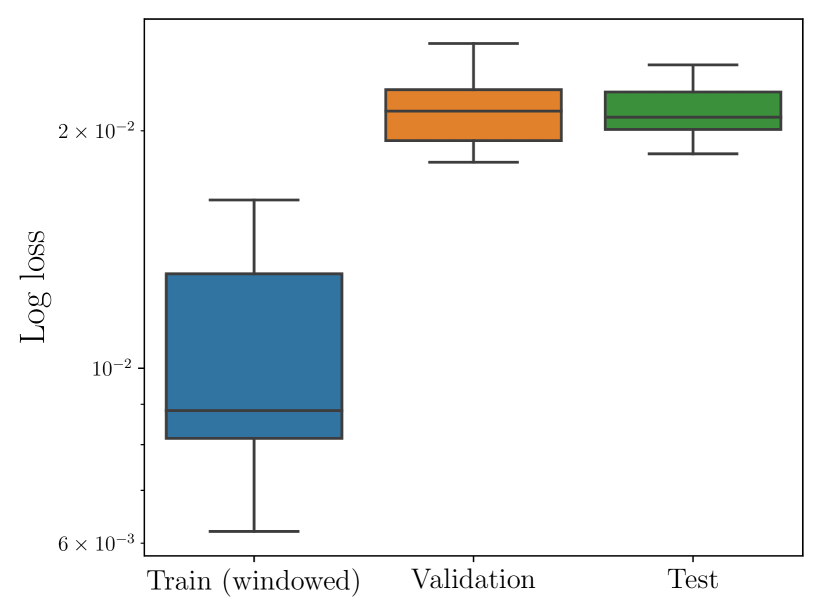
(b)

Figure 3: Plot of the loss distributions for the 10 models trained with data from each system: (a) single fast-spiking neuron; (b) feedforward interconnection of two neurons.

4.2 Feedforward interconnection of two neuron models

Dynamics

We consider a model of the form eq:cond-model-multi with $n=2$. Each of the neurons has $N_{I}=3$ with $I_{1},I_{2}$ as in the previous section and an additional potassium current given by $I_{3}(V,m_{3},n_{3})=g_{3}n_{3}(V-V_{3})$, so that each neuron has 5 states, and thus the interconnection results in a model with 10 states. We take $\epsilon_{12}=0.1$ S, $\epsilon_{21}=0$ S, and $u_{2}\equiv 0$, corresponding to a feedforward interconnection of two regular spiking with adaptation type neurons, as described in Giannari and Astolfi (2022).

Data collection

We follow the procedure described in the previous subsection, collecting 200 trajectories on the time interval $[0,1000]$ ms, with the same distributions for the initial conditions of the membrane voltages and the gating variables, and the same distribution for the current input $u=u_{1}$. The rejection sampling is performed with the density $p(t,x,u)\propto\max_{i=1,2}\tilde{y}_{i}(t,x,u)$.

Architecture and training

The details of the architecture and training procedure are as in the previous section, the sole difference being that the LSTM network now has 32 hidden states.

Results

Figure 2 shows two trajectory predictions with unseen test inputs and initial conditions. As in the previous subsection, we observe that the surrogate model faithfully reproduces the behaviour of the spiking system. Similarly, in Figure 3(b) we verify the robustness of the training procedure with respect to the training parameters.

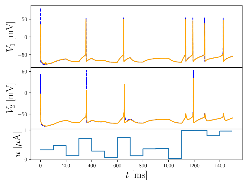
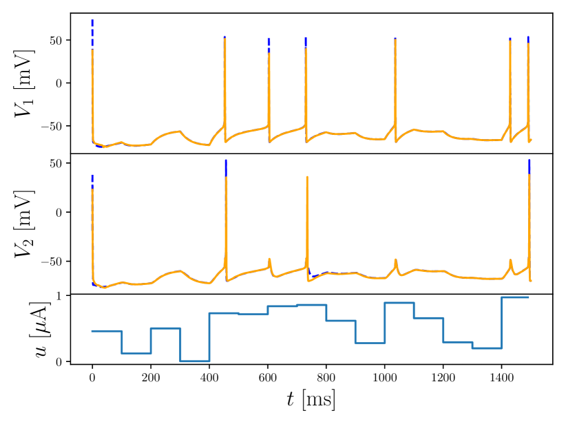
Figure 4: Predictions of output trajectories for the feedforward interconnection of two neurons. The surrogate model prediction is shown in orange; the real output is plotted in blue (dashed).

5 Conclusion

We proposed a framework for surrogate modelling of spiking systems based on approximating the flow function of a class of state-space models exhibiting spiking behaviour. The flow function approximation was performed using an RNN architecture which allows for a direct continuous-time parameterisation of the output trajectories. We discussed two issues which arise when training this architecture on data from a spiking system, namely, the amount of data required to accurately represent the spike signals and the complexity of the optimisation problem, and show how these can be addressed in the context of our method. Finally, we presented results from two numerical experiments which illustrate the feasibility of using our framework for constructing surrogate models of spiking systems.

Directions for future research include an extended experimental study to validate the applicability of the architecture in large networks of spiking systems, and the possibility of further adapting the architecture to enforce system-theoretic properties characteristic of spiking systems. It is also interesting to consider whether surrogate models of complex networks can be obtained in a modular fashion.

This work was supported by the Swedish Research Council Distinguished Professor Grant 2017-01078 and a Knut and Alice Wallenberg Foundation Wallenberg Scholar Grant. The computations were enabled by resources provided by the National Academic Infrastructure for Supercomputing in Sweden (NAISS) at C3SE partially funded by the Swedish Research Council through grant agreement no. 2022-06725.

References

- Aguiar et al. (2023a) Miguel Aguiar, Amritam Das, and Karl H. Johansson. Learning Flow Functions from Data with Applications to Nonlinear Oscillators. IFAC-PapersOnLine, 56(2), 2023a.
- Aguiar et al. (2023b) Miguel Aguiar, Amritam Das, and Karl H. Johansson. Universal approximation of flows of control systems by recurrent neural networks. arXiv e-prints, arXiv:2304.00352, 2023b.
- Beintema et al. (2023) Gerben I. Beintema, Maarten Schoukens, and Roland Tóth. Continuous-time identification of dynamic state-space models by deep subspace encoding. In The Eleventh International Conference on Learning Representations, 2023.
- Biloš et al. (2021) Marin Biloš, Johanna Sommer, Syama S. Rangapuram, Tim Januschowski, and Stephan Günnemann. Neural Flows: Efficient Alternative to Neural ODEs. In Advances in Neural Information Processing Systems, 2021.
- Burghi et al. (2021) Thiago B. Burghi, Maarten Schoukens, and Rodolphe Sepulchre. Feedback identification of conductance-based models. Automatica, 123, 2021.
- Chen et al. (2018) Ricky T. Q. Chen, Yulia Rubanova, Jesse Bettencourt, and David Duvenaud. Neural ordinary differential equations. In Proceedings of the 32nd International Conference on Neural Information Processing Systems, 2018.
- DeWeerth et al. (1991) Stephen P. DeWeerth, Lars Nielsen, Carver A. Mead, and Karl J. Åstrom. A simple neuron servo. IEEE Transactions on Neural Networks, 2(2), 1991.
- Forgione and Piga (2021) Marco Forgione and Dario Piga. Continuous-time system identification with neural networks: Model structures and fitting criteria. European Journal of Control, 59, 2021.
- Giannari and Astolfi (2022) Anastasia G. Giannari and Alessandro Astolfi. Model design for networks of heterogeneous Hodgkin–Huxley neurons. Neurocomputing, 496, 2022.
- Hodgkin and Huxley (1952) Allan L. Hodgkin and Andrew F. Huxley. A quantitative description of membrane current and its application to conduction and excitation in nerve. The Journal of Physiology, 117(4), 1952.
- Kissas et al. (2022) Georgios Kissas, Jacob H. Seidman, Leonardo F. Guilhoto, Victor M. Preciado, George J. Pappas, and Paris Perdikaris. Learning Operators with Coupled Attention. Journal of Machine Learning Research, 23(215), 2022.
- Li et al. (2021) Zongyi Li, Nikola B. Kovachki, Kamyar Azizzadenesheli, Burigede Liu, Kaushik Bhattacharya, Andrew Stuart, and Anima Anandkumar. Fourier Neural Operator for Parametric Partial Differential Equations. In International Conference on Learning Representations, 2021.
- Lin et al. (2023) Guang Lin, Christian Moya, and Zecheng Zhang. Learning the dynamical response of nonlinear non-autonomous dynamical systems with deep operator neural networks. Engineering Applications of Artificial Intelligence, 125, 2023.
- Lu et al. (2021) Lu Lu, Pengzhan Jin, Guofei Pang, Zhongqiang Zhang, and George E. Karniadakis. Learning nonlinear operators via DeepONet based on the universal approximation theorem of operators. Nature Machine Intelligence, 3(3), 2021.
- Mead (1990) Carver A. Mead. Neuromorphic electronic systems. Proceedings of the IEEE, 78(10), 1990.
- Pospischil et al. (2008) Martin Pospischil, Maria Toledo-Rodriguez, Cyril Monier, Zuzanna Piwkowska, Thierry Bal, Yves Frégnac, Henry Markram, and Alain Destexhe. Minimal Hodgkin–Huxley type models for different classes of cortical and thalamic neurons. Biological Cybernetics, 99(4), 2008.
- Qin et al. (2021) Tong Qin, Zhen Chen, John D. Jakeman, and Dongbin Xiu. Data-Driven Learning of Nonautonomous Systems. SIAM Journal on Scientific Computing, 43(3), 2021.
- Ribeiro et al. (2020) Antônio H. Ribeiro, Koen Tiels, Jack Umenberger, Thomas B. Schön, and Luis A. Aguirre. On the smoothness of nonlinear system identification. Automatica, 121, 2020.
- Ross (2013) Sheldon Ross. Chapter 5 - Generating Continuous Random Variables. In Sheldon Ross, editor, Simulation (Fifth Edition). Academic Press, 2013.
- Sepulchre (2022) Rodolphe Sepulchre. Spiking Control Systems. Proceedings of the IEEE, 110(5), 2022.
- Sepulchre et al. (2018) Rodolphe Sepulchre, Guillaume Drion, and Alessio Franci. Excitable behaviors. Emerging Applications of Control and Systems Theory: A Festschrift in Honor of Mathukumalli Vidyasagar, 2018.
- Yang et al. (2022) Alan Yang, Jie Xiong, Maxim Raginsky, and Elyse Rosenbaum. Input-to-State Stable Neural Ordinary Differential Equations with Applications to Transient Modeling of Circuits. In Proceedings of The 4th Annual Learning for Dynamics and Control Conference, 2022.