Sparse is Enough in Fine-tuning Pre-trained Large Language Model

Abstract

With the prevalence of pre-training-fine-tuning paradigm, how to efficiently adapt the pre-trained model to the downstream tasks has been an intriguing issue. Parameter-Efficient Fine-Tuning (PEFT) methods have been proposed for low-cost adaptation, including Adapters, Bia-only, and the recently widely used Low-Rank Adaptation. Although these methods have demonstrated their effectiveness to some extent and have been widely applied, the underlying principles are still unclear. In this paper, we reveal the transition of loss landscape in the downstream domain from random initialization to pre-trained initialization, that is, from low-amplitude oscillation to high-amplitude oscillation. The parameter gradients exhibit a property akin to sparsity, where a small fraction of components dominate the total gradient norm, for instance, 1% of the components account for 99% of the gradient. This property ensures that the pre-trained model can easily find a flat minimizer which guarantees the model’s ability to generalize even with a low number of trainable parameters. Based on this, we propose a gradient-based sparse fine-tuning algorithm, named Sparse Increment Fine-Tuning (SIFT), and validate its effectiveness on a range of tasks including the GLUE Benchmark and Instruction-tuning. The code is accessible at https://github.com/song-wx/SIFT.

1 Introduction

Large Language Models (LLMs) have demonstrated remarkable performance across various tasks. With the prevalent pre-training-fine-tuning paradigm, LLMs can be effectively adapted to the specific downstream domain. As the sizes of pre-trained language models (PLMs) scale up, e.g. GPT-3(Brown et al., 2020) with 175 billion parameters, fine-tuning all the parameters (full fine-tune) has been prohibitively expensive. Therefore, toward efficient adaptation from PLMs to the downstream tasks, several parameter-efficient fine-tuning methods have been proposed, which can match the performance close to or even surpass that of full fine-tuning with a relatively low costs.
Although these methods have demonstrated their effectiveness to some extent and have been widely applied, the underlying principles are still unclear. These methods differ in terms of the selection of trainable parameters and the structure of the trainable modules, but the essence is to train a small set of parameters in order to lead the pre-trained model towards a relatively optimal minimum in downstream domains. This is consistent with (Li et al., 2018a) that over-parameterized networks have a lower intrinsic dimension, i.e. they can achieve 90% or even 100% of the full parameter performance by training only fewer parameters than the full parameter, which is the source of LoRA’s motivation. This has also been verified by numerous PEFT methods, where just fine-tuning a fairly small parameter (e.g. 0.5% of the full parameter) can allow the pre-trained model to be effectively adapted to downstream tasks.
Even though we recognize that the intrinsic dimension of the over-parameterized model is small, in intuition, it is not straightforward to select the correct, appropriate subspace to represent the information of the full space. The existing PEFT methods all go about constructing the subspace heuristically. A unified perspective on the mainstream PEFT methods is given in (He et al., 2022) which argues that from a functional perspective, these methods can all be seen as the form of $down\ projection\to non-linearity\to up\ projection$. To this end, a natural question is:

What is the essence of the low intrinsic dimension of pre-trained language models?

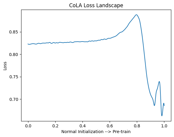
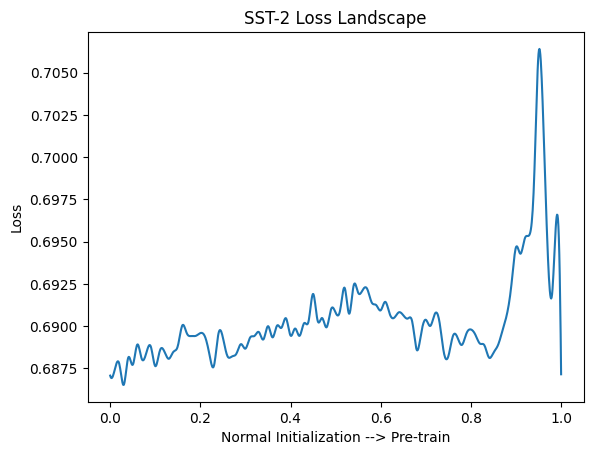
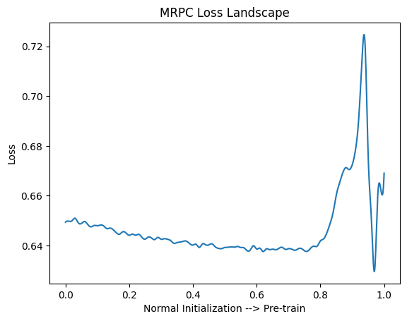
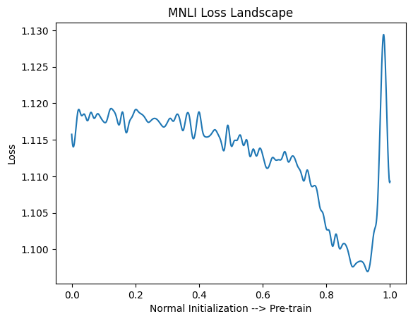
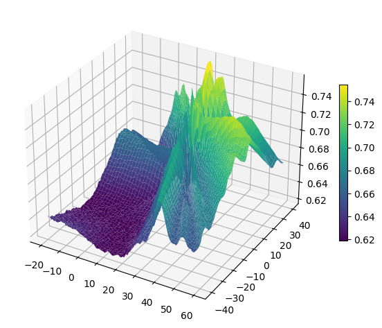
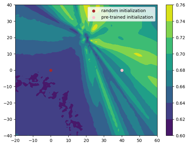
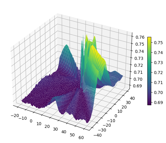
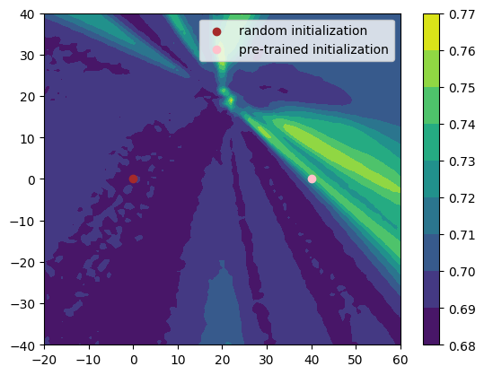
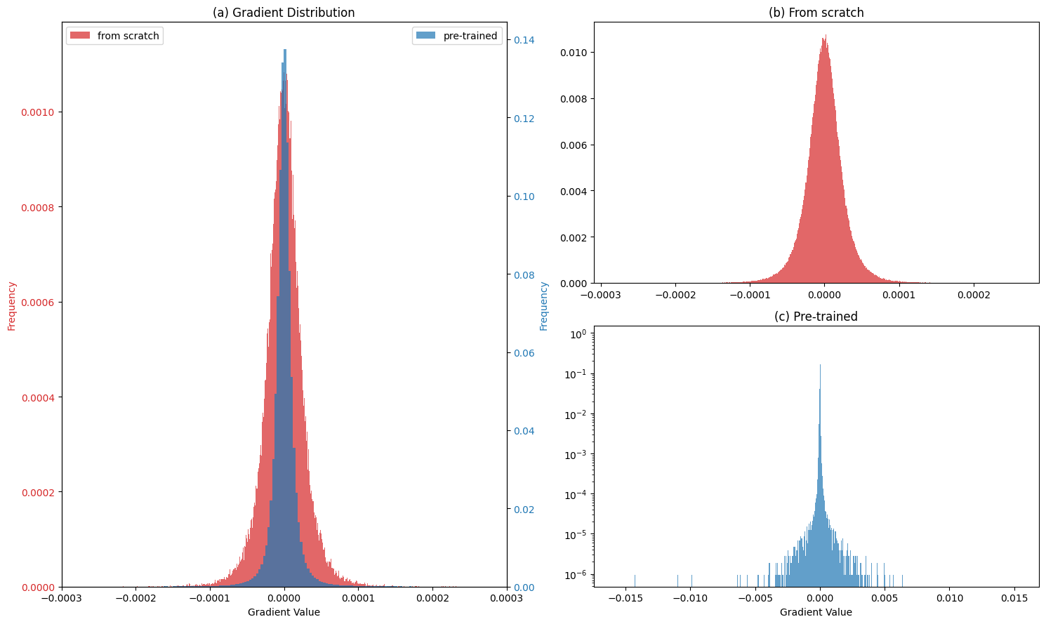
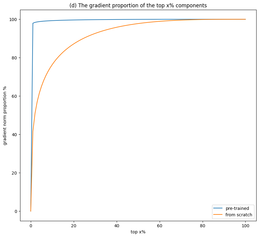
To answer this question, we need to understand what happens during the transition from a randomly initialized model to a pre-trained model. This paper investigates the structure of the loss landscape in downstream domains, viewing the essence of pre-training as guiding the model from a random initialization to a location in the loss landscape with a distinctive structure. We gain an intuitive understanding of this change by visualizing the loss landscape from random parameters to pre-trained parameters. Through one-dimensional and two-dimensional visualizations of the loss landscape, Figure 1 demonstrates a general property: by pretraining, the loss landscape transforms from low-amplitude oscillations near random initialization to high-amplitude oscillations. Corroborating this property, we find that pre-trained models exhibit a sparse-like characteristic in their parameter gradients for downstream tasks, where a small fraction of components account for the majority of the total gradient norm. For example in Figure 2, 1% of the components constitute 99% of the gradient. Hence, we attribute the low intrinsic dimension to this sparse-like property of the gradient space and demonstrate that LoRA’s low-rank structure effectively captures this characteristic. Based on this principle, we propose a gradient-based sparse update algorithm, which involves adding hooks during the backward propagation to acquire a portion of the gradients, thereby achieving both parameter and memory efficient during fine-tuning. We validate its effectiveness on a range of tasks including the GLUE Benchmark and Instruction-tuning.
In summary, the contributions of this paper are as follows:

• To our best knowledge, this is the first time revealing a gradient characteristic widely present in pre-trained models on downstream tasks, where a small fraction of components account for the majority of the gradient norm.

• We propose a gradient-based sparse fine-tuning algorithm, an efficient and simple parameter-efficient fine-tuning method. This approach discards the need for well-designed structures common in various previous PEFT methods, relying only on gradient information to estimate the importance of components and achieving efficient fine-tuning by updating only a part of the components.

• We introduce a memory-efficient sparse fine-tuning approach by utilizing hooks during backward propagation, which could potentially be implemented at the lower level of deep learning training frameworks like PyTorch(Paszke et al., 2017) in the future. This paves the way for more streamlined and efficient fine-tuning, holding considerable potential for widespread application.

2 Related Work

Pre-training-fine-tuning Paradigm: Pre-training models are extensively used in several fields of artificial intelligence, including natural language processing, computer vision and graph learning. Pre-training models learn low-level knowledge by training on large-scale data and thus, from an initialization point of view, pre-training provides better initialization parameters to various downstream tasks. In the field of Natural Language Processing(NLP), language models(LMs) are pre-trained on a large corpus in order to learn rich syntactic and semantic knowledge. There are two main research directions in pre-trained language models (Zhou et al., 2023), one is the autoencoder LMs represented by BERT (Devlin et al., 2019), which learns by training the bi-directional encoders in the Transformer to predict masked words and determine the contextual relationships of sentences. Based on BERT, (Liu et al., 2019) optimized the pre-training method, and in this paper, RoBERTa is used as the backbone model to validate the effectiveness of Sparse Increment Fine-Tuning(SIFT) in the GLUE benchmark.The other is the autoregressive LMs represented by GPT (Radford & Narasimhan, 2018), which extracts the features through autoregressive decoders, and based on the previous words to predict the next word, and fine-tuning on downstream data to solve a specific task. Currently, the majority of the mainstream large language models adopt the autoregressive model with decoder-only, such as Llama (Touvron et al., 2023). In order to allow the LMs to follow human intentions and produce more meaningful content, (Wei et al., 2022) proposes to fine-tune the language model with instructions after pre-training, enabling LMs to align instructions. This paper tests the performance of pre-trained Llama using SIFT for Instruction-tuning.

Figure 1: 1-D (up) and 2-D (down) visualization of the transition of the loss landscape from random initialization to pre-trained initialization. The figures show the loss landscape transitions from low amplitude oscillations to high amplitude oscillations.

Parameter-efficient Fine-tuning: Although the pre-training-fine-tuning paradigm is becoming increasingly popular, the expense of fully fine-tuning large pre-trained models is prohibitively high. (Ding et al., 2022) points out that only 0.5-4% of research papers experimentally adopt large pre-trained models, due to the unaffordable costs of deploying and fine-tuning these large models. To apply pre-trained models more efficiently to downstream tasks, (Houlsby et al., 2019) proposed parameter-efficient transfer learning by inserting a bottleneck structure between different layers of the pre-trained model. During fine-tuning, the pre-trained parameters remain unchanged, and only the bottleneck layers are updated, achieving parameter-efficient fine-tuning. (Zaken et al., 2022) shows that training only the bias terms and task-specific parts of the model during the fine-tuning process can also adapt the pre-trained models effectively to downstream tasks. Prefix-tuning (Li & Liang, 2021) adapts the pre-trained model to downstream tasks by prepending trainable continuous tokens (Prefixes) to the input and hidden states of each Transformer layer. LoRA (Hu et al., 2021) freezes the weights of the pre-trained model and injects trainable rank decomposition matrices into each layer of the Transformer architecture. Following the proposal of LoRA, several LoRA-based improvements have been introduced, including AdaLoRA (Zhang et al., 2023), which adaptively allocates parameter budgets based on the importance of weight matrices, and QLoRA (Dettmers et al., 2023), which further reduces the resource overhead for fine-tuning large pre-trained models through quantization techniques. The above PEFT methods, except for Bias-only which is a module sparse approach, are all adapted to the downstream tasks by introducing additional modules with fewer parameters. In this paper, we present a component sparse approach to achieve almost full fine-tuning performance without introducing additional parameters.

Loss Landscape : Loss landscape is a high-dimensional geometry which is completely determined as soon as a dateset and the network structure are specified(Li et al., 2018a). Our intuition may not be reliable in higher dimension and it is not uncommon for deep learning models of loss landscapes to hold special properties. (Hochreiter & Schmidhuber, 1997) (Keskar et al., 2017) point out that the flatter minima in loss landscape found by stochastic gradient based methods results in better generalization. For the pre-trained models, the flatness of the models on the loss landscape strongly correlates to the performance of the downstream task, even if the pre-training losses are the same (Liu et al., 2022). One approach for analyzing the loss landscape is to visualize this high-dimensional geometry in one or two dimensions. (Li et al., 2018b) visualizes the loss landscape by introducing a ”filter normalization” method, and explains the role of skip connection in terms of the (non)convexity of the loss landscape. (Hao et al., 2019) visualizes the trajectory in the loss landscape during fine-tuning BERT for downstream task and compares the difference between the trajectory of training from scratch and of training from pre-trained model. It is shown that pre-training enables the loss to converge quickly to flatter minima. In this paper, we visualize the transition in loss landscape between random initialization and pre-trained initialization based on the method of (Hao et al., 2019; Li et al., 2018b).

3 Understanding Pre-training-fine-tuning from a Gradient-based Perspective

The pre-training-fine-tuning paradigm has shown great success in numerous NLP tasks (Devlin et al., 2019), to our best knowledge, there is still no conclusive answer as to why pre-training can improve performance and generalization ability in different tasks. In this section we will try to understand the pre-training fine-tuning paradigm from the perspective of gradient distribution along with the visualization of loss landscape.

Figure 2: (a) depicts the gradient distribution of parameters in one layer of RoBERTa-Large on the MNLI dataset, showing different gradient distributions of the models trained from scratch and from pre-trained. Both distribution are approximately presenting a bell-shaped distribution similar to a normal distribution with a mean of zero. (b) and (c) are drawn on their respective scales, showing that compared to the model trained from scratch, the gradients of the pre-trained model are more concentrated around zero while they exists much larger gradient values. (d) illustrates the gradient proportion of the top x% components, indicating that the gradients of the pre-trained model hold a more extreme property, dominating 99% of the complete gradient norm with only 1% of the parameters.

3.1 Visualization of Loss Landscape

Loss landscape is a high-dimensional geometry which is completely determined as soon as a dateset and the network structure are specified(Li et al., 2018a).For high-dimensional geometries such as loss landscapes, it is not possible to imagine and understand their geometric properties as intuitively as in low-dimensional shapes. Despite the difficulty in understanding such high-dimensional geometries, researchers have proposed methods to project high-dimensional loss surfaces into low-dimensional space, including one-dimensional visualization and two-dimensional visualization, in order to easily understand and study some of the properties of loss landscapes. (Hao et al., 2019) first attempts to explain the role of pre-training and fine-tuning in BERT from the perspective of the loss landscape, which visualizes the optimization trajectories both of random initialization and pre-trained initialization in one and two dimensions respectively, giving an intuitive explanation for the faster convergence and better generalization under the pre-training fine-tuning paradigm. However, they treat training from scratch and fine-tuning from pre-trained as two separated cases, ignoring the transition of loss landscape from random initialization to pre-trained initialization. Next, we visualize and explore the transition of loss landscape.

In exploring the transition of the loss landscape from random initialization to pre-trained initialization, we note $\theta_{0}$ as the randomly initialized parameters and $\theta_{1}$ as the pre-trained parameters. (Goodfellow et al., 2015) plots the loss landscape curve from $\theta_{0}$ to $\theta_{1}$ by linearly sampling and interpolating the network parameters between $\theta_{0}$ and $\theta_{1}$, the loss curve $f$ is defined as:

$$f(\alpha) =\mathcal{L}((1-\alpha)\theta_{0}+\alpha\theta_{1})$$

$$=\mathcal{L}(\theta_{0}+\alpha(\theta_{1}-\theta_{0}))$$

$$=\mathcal{L}(\theta_{0}+\alpha\delta)$$

where $\alpha\in[0,1]$ and $\delta$ represents a direction.
The two-dimensional loss surface $f$ is plotted similarly to the one-dimensional one, determined by a starting point and two directions:

$$f(\alpha,\beta)=\mathcal{L}(\theta_{0}+\alpha\delta_{1}+\beta\delta_{2}).$$

In our setting, $\delta_{1}=\theta_{1}-\theta_{0},\alpha\in[-0.5,1.5],\beta\in[-1,1]$, when $\alpha=0,\beta=0$, the model is in the random initialization state, and when $\alpha=1,\beta=0$, the model is in the pre-trained state. We use a method similar to (Li et al., 2018b) to construct the direction $\delta_{2}$ to avoid the scaling effect between different components, multiplying $\delta_{1}$ by a Gaussian random number points by points, i.e. $\delta_{2_{i}}=d_{i}*\delta_{1_{i}},$ where $d_{i}$ follows a normal distribution.
We investigate the transition of the loss landscape using RoBERTa-base(Liu et al., 2019) on a range of tasks at GLUE, some of which are shown in the figure 1. The full results and specific experimental details are given in the Appendix.
A prior idea would be that pre-trained models are more efficient at adapting to downstream tasks than training from scratch because the knowledge learned during pre-training reduces the initial loss. However, a striking fact is that pre-training does not make all tasks have lower losses than random initialization at the beginning of fine-tuning, e.g. MNLI, MRPC, etc. Instead, for most task, there are extremely higher losses than random initialization around the pre-trained initialization. A common feature of the loss landscape across tasks is that the oscillations of the loss around random initialization are generally small in magnitude, whereas the loss oscillations around pre-training are sharp, i.e. after a valid pre-training process, the loss landscape shifts from low amplitude oscillations to high amplitude oscillations. Since the 1-D and 2-D loss landscapes are projections of the original loss landscape, we are curious whether the special properties exhibited in these low-dimensional projections reflect a general property of the high-dimensional space in a statistical sense, that is, whether there is some consistency across most dimensions.

3.2 Quasi-Sparse Gradient Distribution

(Ye et al., 2020; Wiedemann et al., 2020) take the assumption that the distribution of the parameters’ gradients approximates a normal distribution. In the figure 2, we plot the gradient distribution of one parameter in RoBERTa-Large on the MNLI dataset. Both the gradient of the model trained from scratch and from pre-trained show a bell-shaped distribution with a mean of zero. Under the same histogram settings, the gradient distributions of from scratch and pre-trained models show a huge difference in frequency and value range. Figure 2(c) displays the pre-trained gradient distribution on a log-scale, where the majority of gradients are concentrated around zero, with only a very small portion having larger gradient values, and the maximum value of pre-trained is about two orders of magnitude higher than that from scratch. Figure 2(d) shows the gradient proportion of the components with the top x% absolute gradient value. The pre-trained gradient shows a more extreme property, where 1% of the components account for 99% of the total gradient norm. This severe imbalance in distribution exhibits a property similar to sparsity, which we refer to as Quasi-Sparse. The majority of information in the gradient space can be represented by a very small number of components, leading to a low intrinsic dimension of the objective loss landscape(Li et al., 2018a). This imbalance in distribution also explains the transition from low to high amplitude oscillation discussed in 3.1. With the same step size, a balanced distribution of gradients in each dimension would lead a more smooth change in loss, whereas in the case of an imbalanced distribution of gradients, the dimensions with extreme gradients will dominate the change in loss, resulting in strong oscillations.

3.3 Flatter Minima

A popular view is that flatter minima will generalize better(Hochreiter & Schmidhuber, 1997; Jiang et al., 2019; Liu et al., 2022), and for pre-trained models, even with the same pre-training loss, flatter minima have better downstream performance(Liu et al., 2022). (Foret et al., 2021; Bahri et al., 2022) introduce sharpness-aware regularization to reduce the sharpness of the minima during training as a way to improve the generalization ability of the model. For the pre-trained model on the downstream task, whose gradient distribution is akin to sparsity, finding flat minima becomes less difficult, with the flat dimensions dominating the landscape, leaving the sharp dimensions to account for only a very small portion. By stochastic gradient descent methods, it is easy to search for flat minima in a relatively small subspace spanned by the sharp direction, i.e., a minimizer that can sufficiently generalize.

4 Methodology

We describe the design of Sparse Increment Fine-Tuning (SIFT), whose principle is to update only a part of the components of the parameters. Based on the similar subspace method in nonlinear optimization(Liu et al., 2021), we provide a mathematical definition related to SIFT. Finally, we propose a memory-efficient implementation for SIFT.

4.1 SIFT: Sparse Increment Fine-Tuning

We define the fine-tuned parameters as the sum of the pre-trained parameters and an increment, $x_{ft}=x_{pt}+\Delta x.$ Updating only a portion of the components means that $\Delta x$ is a sparse matrix, hence we name this update method Sparse Increment Fine-Tuning (SIFT). Below, we will explain that due to the special gradient properties of the pre-trained model, $\Delta x$ can ensure sufficient descent of the loss.

The idea of only updating partial components of the parameters is similar to the subspace method for non-linear optimization (Liu et al., 2021). In SIFT, we aim to update only the components with the top x% absolute values of the gradient, so the update direction will be in a subspace spanned by these components’ dimensions. We adopt the same definition as in (Liu et al., 2021), where $g_{k}^{i}$ is denoted as the $i^{th}$ component of the gradient $g_{k}$. Sorted in descending order of absolute value, the top x% components are selected, that is:

$$|{g_{k}}^{i_{1}}|\geq|{g_{k}}^{i_{2}}|\geq|{g_{k}}^{i_{3}}|\geq\cdots\geq|{g_{k}}^{i_{m}}|,$$

$$m=[x\%*n],$$

$$n\ is\ the\ number\ of\ g_{k}\ components$$

Therefore, the update direction $d$ are in the subspace $\mathcal{S}=\text{span}\{e^{i_{1}},e^{i_{2}},\ldots,e^{i_{n}}\}$, called the $\tau$-steepest coordinates subspace, where $e_{i}$ refers to the $i^{th}$ standard basis vector. Based on this, we define the steepest descent direction as sufficiently descending, when,

$$\min_{d\in\mathcal{S}}\frac{d^{T}g_{k}}{{\|d\|}_{2}{\|g_{k}\|}_{2}}\leq-\frac{\tau}{n}$$

That is, the descent direction d is sufficiently close to the negative gradient direction. If ${(g_{k}^{\tau+1})}^{2}\leq\epsilon\sum_{j=1}^{\tau}{(g_{k}^{j})}^{2}$, we can further obtain the following estimate,

$$\min_{d\in\mathcal{S}}\frac{d^{T}g_{k}}{{\|d\|}_{2}{\|g_{k}\|}_{2}}\leq-\frac{1}{\sqrt{1+\epsilon(n-\tau)}}$$

As discussed in section 3.2, for the gradients of pre-trained models, a few components dominate most of the gradient norm, allowing us to obtain a sufficiently small $\epsilon$ with a relatively small $\tau$, ensuring that the direction d chosen from the subspace $\mathcal{S}$ is sufficiently descending.

Figure 3: (Left) compares the difference in the proportion of gradients accounted for by two different top 1% component selection methods: the top 1% of the current batch and the top 1% of the first batch. Although sticking with the first batch’s top 1% as opposed to selecting the top 1% of the current batch results in some loss of gradient information, the difference remains within an acceptable range. Avoiding frequent changes of components can improve training efficiency and preserve the historical information of Adam-like optimizers. In contrast, (Right) shows the gradient proportion variation in the model trained from scratch, where fixing the top 1% of the first batch leads to a greater loss of the gradient information.

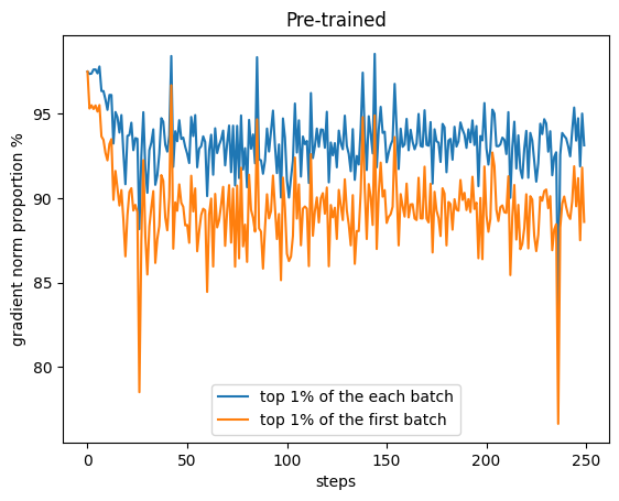
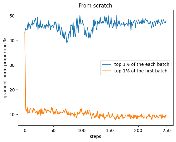
Due to the limitation of computational cost, we usually cannot obtain the gradients over the complete data. Instead, stochastic gradient type methods typically take a mini-batch sampled from the full data. Without the complete gradient information, SIFT uses the gradient from the first batch(or first several batches by using gradient accumulation) as an estimate of the complete gradient and selects the components to be updated based on this. A natural question arises: do the components selected based on the gradient of the first batch still effectively represent the full gradient information in subsequent batches? That is, whether there will be significant differences between the gradients of different batches. As shown in Figure 3, we compare the proportion of the top 1% components of each batch’s gradients with the proportion of the top 1% components of the first batch’s gradients. For pre-trained models, using the top x% components of the first batch does indeed result in some loss of gradient information, but except for some outlier samples, the difference always remains within an acceptable level compared to the top 1% of the current batch. In contrast, the top 1% components of the first batch in models trained from scratch tend to lose more gradient information. Therefore, for efficiency, SIFT always updates the top x% components of the first batch in the whole training process. This approach enables the use of Adam-like optimizers that require historical state information, as frequent changes of components would result in the loss of their historical information. Appropriate periodic changes of the components that need to be updated is also an acceptable choice, and this could be one of the focus for future work.

4.2 A Memory-efficient Implementation of SIFT

Figure 4: (1) For each parameter (P) that requires updating sparsely, we register a Sparse Parameter (SP) with the Sparse Gradient (SG), storing them in the form of values and indexes; (2) Acquire the computed gradient (G) by inserting a hook function; (3) Obtain partial components of the gradient through indexing to serve as the Sparse Gradient for the Sparse Parameter; (4) Use the Sparse Gradient to update the Sparse Parameter in the optimizer; (5) Use the Sparse Parameter to update the initial parameter.

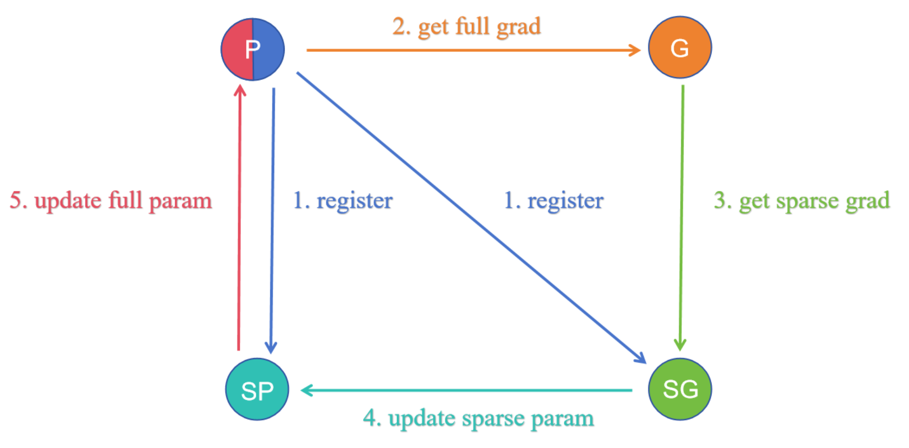
The key to SIFT lies in obtaining the gradients of partial components. Under existing deep learning frameworks (such as PyTorch(Paszke et al., 2017)), gradients of all parameters are able to be accessed only after backward propagation. A simple implementation of SIFT is to retrieve the gradients of partial components through indexing after all gradients have been calculated. However, as all gradients have already been stored, storing the gradients of partial components at this point does not reduce the memory overhead of gradient storage. The memory overhead during training mainly consists of four parts: parameters, gradients, optimizer states, and activations. Although this implementation does not reduce the storage overhead of gradients, it can significantly reduce the storage overhead of the optimizer states.
(Lv et al., 2023) proposes an alternative SGD method that reduces gradient storage by inserting a hook function, thereby fusing the gradient into the parameters as soon as the gradient is computed. Inspired by (Lv et al., 2023), we propose a memory-efficient implementation of SIFT. As shown in Figure 4, we register a Sparse Parameter (SP) and corresponding Sparse Gradient (SG) for the parameters to be updated, storing them in a manner that preserves values and indexes. SP does not obtain Sparse Gradient SG through normal backward propagation. Instead, we inject a hook function into the parameters to capture the computed gradients and assign them to SG via indexing. The Sparse Parameter SP with Sparse Gradient SG is updated through the normal optimizer, and finally, SP is integrated into the initial parameter P.

Table 1: Memory consumption of fine-tuning Llama 7B with different methods including full fine-tuning and SIFT in 5% sparsity rate. The data type of the model is bf16, the optimizers all use AdamW and are in fp32, and the sequence length and batch size are 2048 and 1. GC refers to whether gradient checkpointing is enabled or not.

	GC	Params	Grad	Optim States	Activation	Total
Full	✗	12.55	12.55	50.21	35.72	111.03
	✔				0.81	76.12
SIFT	✗	12.55	0.626	2.51	35.72	51.41
	✔				0.81	16.50

Through this method, for x% sparse updates, we can simultaneously reduce the gradients and optimizer states to the original x%. Combined with techniques such as mixed-precision training and gradient checkpointing, it is possible to fine-tune a 7B model on a single RTX 3090 24GB.

Table 2: Performances of fine-tuned pre-trained RoBERTa-large with different methods on the GLUE benchmark. Num denotes the number of trainable parameters in the fine-tuning process, excluding the classifier. Similar to (Hu et al., 2021), we report the matched and mismatched accuracy for MNLI, Matthew’s correlation for CoLA, Pearson correlation for STS-B, and accuracy for other tasks. * indicates results reported in (Hu et al., 2021). The best results are highlighted in bold and the second best results are underlined.

Model	Method	Num	MNLI	SST-2	MRPC	CoLA	QNLI	QQP	RTE	STS-B	Avg.
RoBERTa-Large	Full*	355.0M	90.2	96.4	90.9	68.0	94.7	92.2	86.6	92.4	88.9
	AdptP*	3.0M	90.2	96.1	90.2	68.3	94.8	91.9	83.8	92.1	88.4
	AdptP*	0.8M	90.5	96.6	89.7	67.8	94.8	91.7	80.1	91.9	87.9
	AdptH*	6.0M	89.9	96.2	88.7	66.5	94.7	92.1	83.4	91.0	87.8
	AdptH*	0.8M	90.3	96.3	87.7	66.3	94.7	91.5	72.9	91.5	86.4
	LoRA*	0.8M	90.6	96.2	90.2	68.2	94.8	91.6	85.2	92.3	88.6
	SIFT	0.8M	90.6	96.2	90.4	68.5	94.1	91.0	85.9	92.3	88.6

5 Experiments

Our evaluation of SIFT mainly consists of two parts, targeting two use cases: Natural Language Understanding (NLU) and Natural Language Generating (NLG). For NLU, we choose to align with the evaluation on LoRA (Hu et al., 2021), selecting the GLUE Benchmark (Wang et al., 2019) as our evaluation dataset, and compare it with the data reported in (Hu et al., 2021). For NLG, to validate the effectiveness of SIFT on much larger models, we choose instruction-tuning as our test case. We select Llama (Touvron et al., 2023) as our backbone models, use the alpaca dataset (Taori et al., 2023) for instruction-tuning, and conduct evaluations on datasets such as MMLU (Hendrycks et al., 2021) and HumanEval (Chen et al., 2021). In the experiment, similar to (Hu et al., 2021), we only consider updating the parameters in the self-attention modules. We further analyze the choice of parameters to update in section 6. By adjusting the sparsity rate of SIFT, we ensure a consistent number of trainable parameters.
In section 5.3, we conduct further experimental analysis towards SIFT. Since SIFT selects components to update through gradient analysis, we compare SIFT with random component selection in section 5.3.2. Additionally, as we heuristically choose to perform sparse updates on q,k,v and o, we compare the specific performance of applying SIFT in different parameters. Finally, we explore the impact of sparsity rate on the downstream task, investigating what is the limit of sparsity rate required for an acceptable performance in the downstream task.
The evaluation includes the following baselines:

• Full fine-tune: All pre-trained parameters are updated.

• Adapter: (Houlsby et al., 2019) proposes to adapt pre-trained models to downstream tasks by inserting trainable Adapter modules into the self-attention layers while keeping the pre-trained parameters frozen. These modules have a bottleneck structure with non-linear function. We denote this original version as $\text{Adpt}^{H}$. Based on (Houlsby et al., 2019), (Pfeiffer et al., 2021) proposed a more efficient version of the Adapter modules, referred to as $\text{Adpt}^{P}$.

• LoRA(Hu et al., 2021): freezes the weights of the pre-trained model and adds trainable rank decomposition matrices in parallel to each layer of the Transformer architecture.

5.1 GLUE Benchmark

We evaluate SIFT on the GLUE benchmark (Wang et al., 2019). We select RoBERTa (Liu et al., 2019) as the backbone model for testing. The general experimental setup is consistent with (Hu et al., 2021) and we apply a 0.8% sparsity rate with SIFT to the Query, Key, Value, and Output projection in the self-attention module to ensure the number of trainable parameters is consistent with the compared baselines. See Appendix for detailed hyperparameter settings. Table 2 reports the results of pre-trained Roberta-large with different fine-tuning methods on the GLUE benchmark and the number of trainable parameters (excluding the classifier). The results of each run are taken from the best epoch. Table 2 reveals that SIFT performs competitive on the GLUE benchmark compared to full fine-tuning and other PEFT methods.

Table 3: Performances of fine-tuned Llama on Alpaca dataset with different methods. We present the accuracy on the MMLU task under zero-shot setting, as well as the pass@1 and pass@10 metrics on the HumanEval task.

Model	Method	Num	MMLU	HumanEval
Llama-7B	Vanilla		32.7	11.3/16.5
	Full	6.74B	42.0	11.1/19.5
	LoRA	0.32B	40.7	11.8/20.1
	SIFT	0.32B	40.7	11.6/20.7
Llama-13B	Vanilla		43.6	14.3/24.4
	Full	13.0B	48.8	15.7/22.0
	LoRA	0.5B	46.7	14.6/25.6
	SIFT	0.5B	46.7	15.5/26.2
Llama-33B	Vanilla		54.3	20.9/36.0
	LoRA	0.98B	55.9	21.6/33.5
	SIFT	0.96B	55.7	24.1/37.2

5.2 Instruction-tuning

(Wei et al., 2022) proposes to perform supervised fine-tuning on top of pre-trained language models to make language models align instructions and generate more meaningful content. (Taori et al., 2023) fine-tunes the pre-trained Llama on a 52k instruction-following dataset (Alpaca), which is generated by the technique introduced in (Wang et al., 2023). We fine-tune llama with Alpaca in different ways including full fine-tuning, LoRA and our SIFT. We evaluate the language model on multiple benchmarks including MMLU and HumanEval. For MMLU, the evaluation metric is the accuracy of the generating answer in zero-shot setting, while the code evaluation task HumanEval is evaluated by the pass@1 and pass@10 metric. Higher values are better for all metrics. Detailed experimental hyper-parameters are described in the Appendix. Table 3 demonstrates that sparse structures like SIFT can inject knowledge into the pre-trained large language models and exhibit competitive performance.

5.3 Further Analysis

In this subsection, we primarily conduct further experimental analysis towards SIFT. This involves comparing the performance differences when applying SIFT on different parameters, as well as the differences between SIFT’s gradient-based component selection and random selection. Finally, we discuss the impact of the sparsity rate on the performance of downstream tasks.

5.3.1 SIFT Vs Random

SIFT selects the component with the highest absolute gradient value in the first batch for the subsequent updates. A natural question arises: does the selection method of SIFT have an advantage over random selection? Additionally, in previous experiments, we heuristically choose the $W_{q},W_{k},W_{v}$ and $W_{o}$ in the attention modules for sparse updating. Under the condition of maintaining the same number of trainable parameters, including more modules to apply SIFT means that each module has fewer components available for updates. We want to know whether having fewer modules with more components or more modules with fewer components performs better in the fine-tuning process. In Table 4, we compare the performance of SIFT and random selection in updating different modules. We choose two small datasets from the GLUE benchmark, RTE and MRPC, for evaluation. The final performances do not show a consistent conclusion in the choice of different update modules. Therefore, balancing the number of components and modules, we choose to update $W_{q},W_{k},W_{v}$ and $W_{o}$ as our final choice. Compared to random selection, SIFT’s gradient-based selection method shows a clear advantage in the final performance of downstream tasks. However, unexpectedly, although not as effective as SIFT in terms of performances, sparse updates in randomly selected components can still effectively adapt pre-trained models to downstream tasks, with only a small performance gap. One hypothesis is that the property of sparsity is broadly present in pre-trained models, with quasi-sparse gradients being just one of its important representations, which still requires further research.

Table 4: Performances of applying SIFT and random selection on different parameters. $W_{q},W_{k},W_{v},W_{o}$ represent the query, key, value, and output parameters in the attention module respectively and $W_{All}$ denotes all parameters in the attention module (excluding LayerNorm).

Type	Weight	Num	RTE	MRPC	Avg.
SIFT	$W_{V}$	0.81M	85.9	90.4	88.0
	$W_{Q,V}$	0.81M	85.2	90.2	87.7
	$W_{Q,K,V}$	0.83M	84.8	88.7	86.8
	$W_{Q,K,V,O}$	0.80M	85.9	90.4	88.0
	$W_{All}$	0.80M	86.6	89.0	87.8
Random	$W_{V}$	0.81M	83.0	89.2	86.1
	$W_{Q,V}$	0.81M	82.3	89.0	85.7
	$W_{Q,K,V}$	0.83M	81.9	87.5	84.7
	$W_{Q,K,V,O}$	0.80M	83.8	89.5	86.5
	$W_{All}$	0.80M	83.0	88.2	85.6

5.3.2 Sparsity Rate Analysis

Figure 5: Performances of the fine-tuned pre-trained RoBERTa-Large vs different methods and the numbers of trainable parameters. Classifier only indicates that only the classifiers are fine-tuned, and the rest of the methods update the classifiers along with the parts of the pre-trained model.

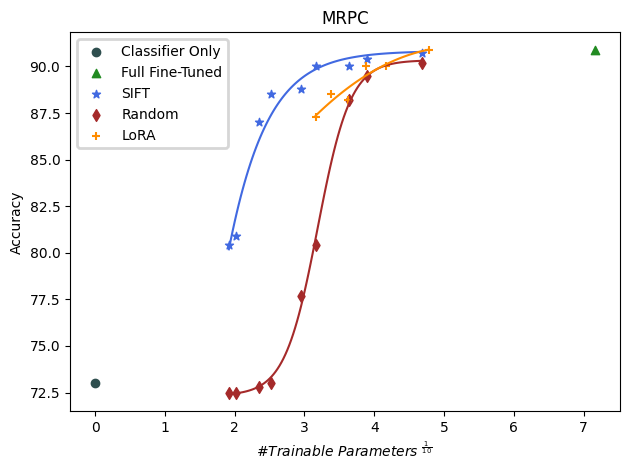
We test the efficiency of different methods, that is, the trend of performance with the number of trainable parameters. We compare SIFT, Random selection and LoRA with varied numbers of trainable parameters on the MRPC task. The results show that SIFT is able to adapt the downstream task more efficiently with smaller parameters, while the performance gap between SIFT and LoRA is smoothed out as the number of parameters increases. Consistent with the conclusion of 5.3.1, we find that when the number of parameters reaches a certain threshold, Random is also able to adapt the downstream task, but it is significantly inferior to SIFT and LoRA in terms of the performances for small parameters.

6 Conclusion

In this paper, we reveal the gradient properties of pre-trained language models on downstream domains. By visualizing the loss landscape and the gradient distribution, we find that the gradients of pre-trained models exhibit a sparse-like property, which we refer to as the Quasi-Sparse gradient distribution. Based on this, we introduce a component-sparse fine-tuning paradigm named SIFT, which differs from previous parameter-efficient fine-tuning methods that involve injecting small plug-ins (such as Adapters and LoRA) or module-sparsity (such as Bias-only), and propose a memory-efficient implementation. This method is a more streamlined approach for fine-tuning, and experiments demonstrate that it is on par with the mainstream PEFT methods.

Limitation

Although we have discovered that the gradients of pre-trained models on downstream tasks exhibit a quasi-sparse nature, the specific reasons for this are not yet clear. How to utilize this feature to aid in better pre-training will be a viable direction. Meanwhile, the selection of modules to update remains heuristic, and whether the selection of modules and allocation of component quotas can also be done through gradients is a question worth researching. In this paper, we present a memory-efficient implementation of SIFT but It must be acknowledged that our implementation currently only supports training on a single card and that the training speed significantly decreases with the increase of the sparsity rate. How to implement SIFT more efficiently remains an unresolved issue.

References

- Bahri et al. (2022) Bahri, D., Mobahi, H., and Tay, Y. Sharpness-aware minimization improves language model generalization, 2022.
- Brown et al. (2020) Brown, T. B., Mann, B., Ryder, N., Subbiah, M., Kaplan, J., Dhariwal, P., Neelakantan, A., Shyam, P., Sastry, G., Askell, A., Agarwal, S., Herbert-Voss, A., Krueger, G., Henighan, T., Child, R., Ramesh, A., Ziegler, D. M., Wu, J., Winter, C., Hesse, C., Chen, M., Sigler, E., Litwin, M., Gray, S., Chess, B., Clark, J., Berner, C., McCandlish, S., Radford, A., Sutskever, I., and Amodei, D. Language models are few-shot learners, 2020.
- Chen et al. (2021) Chen, M., Tworek, J., Jun, H., Yuan, Q., de Oliveira Pinto, H. P., Kaplan, J., Edwards, H., Burda, Y., Joseph, N., Brockman, G., Ray, A., Puri, R., Krueger, G., Petrov, M., Khlaaf, H., Sastry, G., Mishkin, P., Chan, B., Gray, S., Ryder, N., Pavlov, M., Power, A., Kaiser, L., Bavarian, M., Winter, C., Tillet, P., Such, F. P., Cummings, D., Plappert, M., Chantzis, F., Barnes, E., Herbert-Voss, A., Guss, W. H., Nichol, A., Paino, A., Tezak, N., Tang, J., Babuschkin, I., Balaji, S., Jain, S., Saunders, W., Hesse, C., Carr, A. N., Leike, J., Achiam, J., Misra, V., Morikawa, E., Radford, A., Knight, M., Brundage, M., Murati, M., Mayer, K., Welinder, P., McGrew, B., Amodei, D., McCandlish, S., Sutskever, I., and Zaremba, W. Evaluating large language models trained on code, 2021.
- Dettmers et al. (2023) Dettmers, T., Pagnoni, A., Holtzman, A., and Zettlemoyer, L. Qlora: Efficient finetuning of quantized llms, 2023.
- Devlin et al. (2019) Devlin, J., Chang, M.-W., Lee, K., and Toutanova, K. Bert: Pre-training of deep bidirectional transformers for language understanding, 2019.
- Ding et al. (2022) Ding, N., Qin, Y., Yang, G., Wei, F., Yang, Z., Su, Y., Hu, S., Chen, Y., Chan, C.-M., Chen, W., Yi, J., Zhao, W., Wang, X., Liu, Z., Zheng, H.-T., Chen, J., Liu, Y., Tang, J., Li, J., and Sun, M. Delta tuning: A comprehensive study of parameter efficient methods for pre-trained language models, 2022.
- Foret et al. (2021) Foret, P., Kleiner, A., Mobahi, H., and Neyshabur, B. Sharpness-aware minimization for efficiently improving generalization, 2021.
- Goodfellow et al. (2015) Goodfellow, I. J., Vinyals, O., and Saxe, A. M. Qualitatively characterizing neural network optimization problems, 2015.
- Hao et al. (2019) Hao, Y., Dong, L., Wei, F., and Xu, K. Visualizing and understanding the effectiveness of bert, 2019.
- He et al. (2022) He, J., Zhou, C., Ma, X., Berg-Kirkpatrick, T., and Neubig, G. Towards a unified view of parameter-efficient transfer learning, 2022.
- Hendrycks et al. (2021) Hendrycks, D., Burns, C., Basart, S., Zou, A., Mazeika, M., Song, D., and Steinhardt, J. Measuring massive multitask language understanding, 2021.
- Hochreiter & Schmidhuber (1997) Hochreiter, S. and Schmidhuber, J. Flat Minima. Neural Computation, 9(1):1–42, 01 1997. ISSN 0899-7667. doi: 10.1162/neco.1997.9.1.1. URL https://doi.org/10.1162/neco.1997.9.1.1.
- Houlsby et al. (2019) Houlsby, N., Giurgiu, A., Jastrzebski, S., Morrone, B., de Laroussilhe, Q., Gesmundo, A., Attariyan, M., and Gelly, S. Parameter-efficient transfer learning for nlp, 2019.
- Hu et al. (2021) Hu, E. J., Shen, Y., Wallis, P., Allen-Zhu, Z., Li, Y., Wang, S., Wang, L., and Chen, W. Lora: Low-rank adaptation of large language models, 2021.
- Jiang et al. (2019) Jiang, Y., Neyshabur, B., Mobahi, H., Krishnan, D., and Bengio, S. Fantastic generalization measures and where to find them, 2019.
- Keskar et al. (2017) Keskar, N. S., Mudigere, D., Nocedal, J., Smelyanskiy, M., and Tang, P. T. P. On large-batch training for deep learning: Generalization gap and sharp minima, 2017.
- Li et al. (2018a) Li, C., Farkhoor, H., Liu, R., and Yosinski, J. Measuring the intrinsic dimension of objective landscapes, 2018a.
- Li et al. (2018b) Li, H., Xu, Z., Taylor, G., Studer, C., and Goldstein, T. Visualizing the loss landscape of neural nets, 2018b.
- Li & Liang (2021) Li, X. L. and Liang, P. Prefix-tuning: Optimizing continuous prompts for generation, 2021.
- Liu et al. (2022) Liu, H., Xie, S. M., Li, Z., and Ma, T. Same pre-training loss, better downstream: Implicit bias matters for language models, 2022.
- Liu et al. (2021) Liu, X., Wen, Z., Yuan, and Ya-Xiang. Subspace methods for nonlinear optimization. CSIAM Transactions on Applied Mathematics, 2(4):585–651, 2021. ISSN 2708-0579. doi: https://doi.org/10.4208/csiam-am.SO-2021-0016. URL http://global-sci.org/intro/article_detail/csiam-am/19986.html.
- Liu et al. (2019) Liu, Y., Ott, M., Goyal, N., Du, J., Joshi, M., Chen, D., Levy, O., Lewis, M., Zettlemoyer, L., and Stoyanov, V. Roberta: A robustly optimized bert pretraining approach, 2019.
- Lv et al. (2023) Lv, K., Yang, Y., Liu, T., Gao, Q., Guo, Q., and Qiu, X. Full parameter fine-tuning for large language models with limited resources, 2023.
- Paszke et al. (2017) Paszke, A., Gross, S., Chintala, S., Chanan, G., Yang, E., DeVito, Z., Lin, Z., Desmaison, A., Antiga, L., and Lerer, A. Automatic differentiation in pytorch. 2017.
- Pfeiffer et al. (2021) Pfeiffer, J., Kamath, A., Rücklé, A., Cho, K., and Gurevych, I. Adapterfusion: Non-destructive task composition for transfer learning, 2021.
- Radford & Narasimhan (2018) Radford, A. and Narasimhan, K. Improving language understanding by generative pre-training. 2018. URL https://api.semanticscholar.org/CorpusID:49313245.
- Taori et al. (2023) Taori, R., Gulrajani, I., Zhang, T., Dubois, Y., Li, X., Guestrin, C., Liang, P., and Hashimoto, T. B. Stanford alpaca: An instruction-following llama model. https://github.com/tatsu-lab/stanford_alpaca, 2023.
- Touvron et al. (2023) Touvron, H., Lavril, T., Izacard, G., Martinet, X., Lachaux, M.-A., Lacroix, T., Rozière, B., Goyal, N., Hambro, E., Azhar, F., Rodriguez, A., Joulin, A., Grave, E., and Lample, G. Llama: Open and efficient foundation language models, 2023.
- Wang et al. (2019) Wang, A., Singh, A., Michael, J., Hill, F., Levy, O., and Bowman, S. R. Glue: A multi-task benchmark and analysis platform for natural language understanding, 2019.
- Wang et al. (2023) Wang, Y., Kordi, Y., Mishra, S., Liu, A., Smith, N. A., Khashabi, D., and Hajishirzi, H. Self-instruct: Aligning language models with self-generated instructions, 2023.
- Wei et al. (2022) Wei, J., Bosma, M., Zhao, V. Y., Guu, K., Yu, A. W., Lester, B., Du, N., Dai, A. M., and Le, Q. V. Finetuned language models are zero-shot learners, 2022.
- Wiedemann et al. (2020) Wiedemann, S., Mehari, T., Kepp, K., and Samek, W. Dithered backprop: A sparse and quantized backpropagation algorithm for more efficient deep neural network training, 2020.
- Ye et al. (2020) Ye, X., Dai, P., Luo, J., Guo, X., Qi, Y., Yang, J., and Chen, Y. Accelerating cnn training by pruning activation gradients, 2020.
- Zaken et al. (2022) Zaken, E. B., Ravfogel, S., and Goldberg, Y. Bitfit: Simple parameter-efficient fine-tuning for transformer-based masked language-models, 2022.
- Zhang et al. (2023) Zhang, Q., Chen, M., Bukharin, A., He, P., Cheng, Y., Chen, W., and Zhao, T. Adaptive budget allocation for parameter-efficient fine-tuning, 2023.
- Zhou et al. (2023) Zhou, C., Li, Q., Li, C., Yu, J., Liu, Y., Wang, G., Zhang, K., Ji, C., Yan, Q., He, L., Peng, H., Li, J., Wu, J., Liu, Z., Xie, P., Xiong, C., Pei, J., Yu, P. S., and Sun, L. A comprehensive survey on pretrained foundation models: A history from bert to chatgpt, 2023.