Abstract

Formal abductive explanations offer crucial guarantees of rigor and so are of interest in high-stakes uses of machine learning (ML). One drawback of abductive explanations is explanation size, justified by the cognitive limits of human decision-makers. Probabilistic abductive explanations (PAXps) address this limitation, but their theoretical and practical complexity makes their exact computation most often unrealistic. This paper proposes novel efficient algorithms for the computation of locally-minimal PXAps, which offer high-quality approximations of PXAps in practice. The experimental results demonstrate the practical efficiency of the proposed algorithms.

1 Introduction

Formal abductive explanations are justified by the need of guarantees of rigor in high-stakes uses of machine learning (ML) [Marques-Silva and Ignatiev, 2022]. One drawback of abductive explanations is explanation size, given the cognitive limits of human decision-makers [Miller, 1956]. Probabilistic abductive explanations [Wäldchen et al., 2021] represent one possible solution for finding explanations of smaller size, where the trade off is between explanation size and strong theoretical guarantees on the quality of approximate explanations. Unfortuantely, the complexity of finding probabilistic abductive explanations is in general unwiedly [Wäldchen et al., 2021], e.g. a practical algorithm should be expected to call a counting oracle exponentially many times. Even for restricted families of classifiers, e.g. decision trees, it is known that the computation of probabilistic abductive explanations is computationally hard, albeit solvable with a limited number of calls to an NP-oracle [Arenas et al., 2022, Izza et al., 2023]. Clearly, the case of decision trees, while still computationally hard, is drastically easier to solve in practice.

One key difficulty in computing probabilistic abductive explanations results from the non-monotonicity of the sets representing or not a probabilistic explanation. This lack of monotonicity requires the analysis of all possible subsets of features in order to find a subset-minimal set. In such a situation, one approximation to subset-minimality is local minimality, i.e. sets that are minimal if at most one feature is allowed to be removed. A surprising experimental observation [Izza et al., 2023] is that, in the case of decision trees and other graph-based classifiers, locally-minimal explanations are in most cases also subset-minimal explanations — reported results show for decision trees that in 99.8% cases computed approximate explanations are proved that are subset minimal.

Given these earlier experimental observations, one solution towards devising practical algorithms for approximating probabilistic abductive explanations is to compute locally-minimal explanations, thereby eliminating the need to analyze all possible subsets of a target set of features. This paper proposes two new algorithms for computing approximate locally-minimal explanations, one based on approximate model counting, and the other based on sampling with probabilistic guarantees. The experimental results support the practical efficiency of the proposed algorithms for two case study classifiers random forest (RF) and binarized neural network (BNN) — results on BNNs show that explanation length of our solution drops by one third to two third of abductive explanation size.

The paper is organized as follows. Section 2 introduces the notation and definitions used in the paper. Section 3 overviews the logic encodings of classifiers used in later sections. Section 4 describes the approach proposed in this paper. The experimental results are discussed in Section 5. Finally, the paper concludes in Section 6.

2 Preliminaries

Classification problems.

This paper considers classification problems, which are defined on a set of features (or attributes) ${\mathcal{F}}=\{1,\ldots,m\}$ and a set of classes ${\mathcal{K}}=\{c_{1},c_{2},\ldots,c_{K}\}$. Each feature $i\in{\mathcal{F}}$ takes values from a domain $\mathbb{D}_{i}$. In general, domains can be categorical or ordinal, with values that can be boolean, integer or real-valued. Feature space is defined as $\mathbb{F}=\mathbb{D}_{1}\times{\mathbb{D}_{2}}\times\ldots\times{\mathbb{D}_{m}}$; $|\mathbb{F}|$ represents the total number of points in $\mathbb{F}$. For boolean domains, $\mathbb{D}_{i}=\{0,1\}=\mathbb{B}$, $i=1,\ldots,m$, and $\mathbb{F}=\mathbb{B}^{m}$. The notation $\mathbf{x}=(x_{1},\ldots,x_{m})$ denotes an arbitrary point in feature space, where each $x_{i}$ is a variable taking values from $\mathbb{D}_{i}$. The set of variables associated with features is $X=\{x_{1},\ldots,x_{m}\}$. Moreover, the notation $\mathbf{v}=(v_{1},\ldots,v_{m})$ represents a specific point in feature space, where each $v_{i}$ is a constant representing one concrete value from $\mathbb{D}_{i}$. An ML classifier $\mathbb{M}$ is characterized by a (non-constant) classification function $\kappa$ that maps feature space $\mathbb{F}$ into the set of classes ${\mathcal{K}}$, i.e. $\kappa:\mathbb{F}\to{\mathcal{K}}$. An instance denotes a pair $(\mathbf{v},c)$, where $\mathbf{v}\in\mathbb{F}$ and $c\in{\mathcal{K}}$, with $c=\kappa(\mathbf{v})$.

Random Forests (RFs).

Random Forests (RFs) [Breiman, 2001, Yang et al., 2020, Zhang et al., 2019, Gao and Zhou, 2020, Feng and Zhou, 2018, Zhou and Feng, 2017] are an example of tree ensemble ML models, which find a wide range of practical applications. Although RFs are known to lack in interpretability, recent work [Izza and Marques-Silva, 2021, Ignatiev et al., 2022a] demonstrates that large tree ensembles can be efficiently analyzed with logical-based reasoners like SAT/SMT oracles, and so can be explained. Conceptually, an RF is collection of decision trees (DTs), where each tree ${\mathcal{T}}_{i}$, $i\in\{1,\dots,T\}$ of the ensemble ${\mathcal{T}}$ is trained on a randomly selected subset of the training data so that the trees of the RF are not correlated. (In contrast to a single DT, RFs are less prone to over-fitting and so offer in general better accuracy on test data [Breiman, 2001].) Similar to the original proposal for RFs [Breiman, 2001], the predictions of a RF classifier are made by majority vote of trees, that is each tree predicts for a class and the class with largest score is picked. Other solutions could be considered, e.g. weighted voting.

Binarized Neural Network (BNNs).

Binarized Neural Networks (BNNs) [Hubara et al., 2016, Courbariaux et al., 2016] are a widely used family of neural networks. BNNs exhibit a number of important features that allow them to be deployed into embedded devices [McDanel et al., 2017, Kung et al., 2018]. Concretely, a BNN is composed of a number of layers of neurons. The neurons of the intermediate layers (hidden layers) compute a mapping function: $\{-1,1\}^{n}\rightarrow\{-1,1\}^{m}$ on input $x_{i}\in\{-1,1\}^{n}$, whilst the neurons of the last layer (output layer) map a binary tensor to real domain: $\{-1,1\}^{n_{d}}\rightarrow\mathbb{R}^{K}$ on input $x_{i}\in\{-1,1\}^{n_{d}}$. Furthermore, outputs of intermediate layer are obtained with applying three transformations on the input tensor $x$: a linear transformation (LIN), batch normalization (BatchNorm) and binarization (BIN), such that $x^{i+1}=\textsc{Bin}(\textsc{BatchNorm}(\textsc{Lin}(x)))$, where: Lin($x^{i}$) = $W^{i}x^{i}+b^{i}$, where $W^{i}\in\{-1,1\}^{m\times n}$ and $b^{i}\in\mathbb{R}^{n}$, BatchNorm($y_{j}$) = $\alpha^{i}_{j}\left(\frac{y_{j}-\mu_{j}^{i}}{\sigma^{i}_{j}}\right)$, where $\alpha^{i}_{j},\mu_{j}^{i},\sigma^{i}_{j},y_{j}\in\mathbb{R}^{m}$, and Bin($z$) = $sign(z)\in\{-1,1\}^{m}$. Lastly, the output layer applies a linear transformation before softmax/argmax mapping that picks a class to predict. (Note that [Narodytska et al., 2020, Jia and Rinard, 2020] propose to use ternary neural network in order to generate sparse matrices, hence we have $W^{i}\in\{-1,0,1\}$. )

Abductive explanations.

Prime implicant (PI) explanations [Shih et al., 2018] denote a minimal set of literals (relating a feature value $x_{i}$ and a constant $v_{i}\in\mathbb{D}_{i}$) that are sufficient for the prediction. PI-explanations are related with abduction, and so are also referred to as abductive explanations (AXp’s) [Ignatiev et al., 2019]. Formally, given $\mathbf{v}=(v_{1},\ldots,v_{m})\in\mathbb{F}$ with $\kappa(\mathbf{v})=c$, a set of features ${\mathcal{X}}\subseteq{\mathcal{F}}$ is a weak abductive explanation [Cooper and Marques-Silva, 2021] (or weak AXp) if the following predicate holds true:

$$\mathsf{WeakAXp}({\mathcal{X}})\>{:=}~{} \forall(\mathbf{x}\in\mathbb{F}).$$

$$\left[\bigwedge\nolimits_{i\in{{\mathcal{X}}}}(x_{i}=v_{i})\right]\operatorname*{\rightarrow}(\kappa(\mathbf{x})=c)$$ (1)

The classifier assigns the same class to all feature-vectors which agree with $\mathbf{v}$ on features in a weak AXp ${\mathcal{X}}$. Such sets ${\mathcal{X}}$ may contain features which do not contribute to the decision, which leads to the following definition. A set of features ${\mathcal{X}}\subseteq{\mathcal{F}}$ is an abductive explanation (or (plain) AXp) if the following predicate holds true:

$$\mathsf{AXp}({\mathcal{X}})\quad{:=}\quad \mathsf{WeakAXp}({\mathcal{X}})~{}\land$$

$$\forall({\mathcal{X}}^{\prime}\subsetneq{\mathcal{X}}).\neg\mathsf{WeakAXp}({\mathcal{X}}^{\prime})$$ (2)

Clearly, an AXp is any weak AXp that is subset-minimal (or irrreducible). It is straightforward to observe that the definition of predicate $\mathsf{WeakAXp}$ is monotone, and so an AXp can instead be defined as follows:

$$\mathsf{AXp}({\mathcal{X}})\quad{:=}\quad \mathsf{WeakAXp}({\mathcal{X}};)~{}\land$$

$$\forall(j\in{\mathcal{X}}).\neg\mathsf{WeakAXp}({\mathcal{X}}\setminus\{j\})$$ (3)

(Throughout the document, we will drop the parameterization associated with each predicate, and so we will write $\mathsf{AXp}({\mathcal{X}})$ instead of $\mathsf{AXp}({\mathcal{X}})$, when the parameters are clear from the context.)

Logic-based explainability is covered in a number of recent works. Explaining tree ensembles is studied in [Izza and Marques-Silva, 2021, Ignatiev et al., 2022b]. Probabilistic explanations are investigated in [Wäldchen et al., 2021, Arenas et al., 2022, Izza et al., 2023].

Probabilistic AXp’s.

A weak probabilistic AXp (or weak PAXp) is a pick of fixed features for which the conditional probability of predicting the correct class $c$ exceeds $\mathrm{T}$, given $c=\kappa(\mathbf{v})$. Thus, ${\mathcal{X}}\subseteq{\mathcal{F}}$ is a weak PAXp if the following predicate holds true,

$$\mathsf{WeakPAXp} ({\mathcal{X}})$$

$$:=\,\> \textnormal{Pr}_{\mathbf{x}}(\kappa(\mathbf{x})=c\,|\,\mathbf{x}_{{\mathcal{X}}}=\mathbf{v}_{{\mathcal{X}}})\geq\mathrm{T}$$ (4)

$$:=\,\> \frac{|\{\mathbf{x}\in\mathbb{F}:\kappa(\mathbf{x})=c\land(\mathbf{x}_{{\mathcal{X}}}=\mathbf{v}_{{\mathcal{X}}})\}|}{|\{\mathbf{x}\in\mathbb{F}:(\mathbf{x}_{{\mathcal{X}}}=\mathbf{v}_{{\mathcal{X}}})\}|}\geq\mathrm{T}$$

which means that the fraction of the number of points predicting the target class and consistent with the fixed features (represented by ${\mathcal{X}}$), given the total number of points in feature space consistent with the fixed features, must exceed $\mathrm{T}$. Moreover, a set ${\mathcal{X}}\subseteq{\mathcal{F}}$ is a probabilistic AXp (or (plain) PAXp) if the following predicate holds true,

$$\mathsf{PAXp} ({\mathcal{X}})\>:=$$

$$\mathsf{WeakPAXp}({\mathcal{X}})\>\>\land$$ (5)

$$\forall({\mathcal{X}}^{\prime}\subsetneq{\mathcal{X}}).\neg\mathsf{WeakPAXp}({\mathcal{X}}^{\prime})$$

Thus, ${\mathcal{X}}\subseteq{\mathcal{F}}$ is a PAXp if it is a weak PAXp that is also subset-minimal,

As can be observed, the definition of weak PAXp (see Eq. (2)) does not guarantee monotonicity. In turn, this makes the computation of (subset-minimal) PAXp’s harder. With the purpose of identifiying classes of weak PAXp’s that are easier to compute, it will be convenient to study locally-minimal PAXp’s. A set of features ${\mathcal{X}}\subseteq{\mathcal{F}}$ is a locally-minimal PAXp if,

$$\mathsf{LmPAXp} ({\mathcal{X}})\>:=$$

$$\mathsf{WeakPAXp}({\mathcal{X}})\>\>\land$$ (6)

$$\forall(j\in{\mathcal{X}}).\neg\mathsf{WeakPAXp}({\mathcal{X}}\setminus\{j\})$$

As observed earlier, because the predicate $\mathsf{WeakAXp}$ is monotone, subset-minimal AXp’s match locally-minimal AXp’s. An important practical consequence is that most algorithms for computing one subset-minimal AXp, will instead compute a locally-minimal AXp, since these will be the same. Nevertheless, a critical observation is that in the case of probabilistic AXp’s (see Eq. (2)), the predicate $\mathsf{WeakPAXp}$ is not monotone. Thus, there can exist locally-minimal PAXp’s that are not subset-minimal PAXp’s.

3 Logic Encodings

In this section we detail the encodings for both random forests (with majority voting) and binarized neural networks. It should be noted that the proposed declarative encodings on both random forests and binarized neural networks are polynomial on the size of the original ML classifier.

RF Encoding.

We adapt the propositional encoding of RFs proposed in [Izza and Marques-Silva, 2021] to encode $\kappa(\mathbf{x})$ entails the prediction of input $\mathbf{v}$, in order to be able to compute the number of models satisfying this entailment. Concretely, we need to encode the RF structure (i.e. trees and feature-domain encodings) and the prediction function $\kappa(\mathbf{x})$ (i.e. majority vote of the ensemble model) into a SAT problem. As results, each tree ${\mathcal{T}}_{i}$ of the model is encoded as a set of implications expressing the paths ${\mathcal{P}}_{i}$ of ${\mathcal{T}}_{i}$, as follow: $\operatorname*{\bigvee}\nolimits_{P\in{\mathcal{P}}_{i}}\left(\operatorname*{\bigvee}\nolimits_{l\in\Lambda(P)}l\operatorname*{\leftrightarrow}p_{ij}\right)$, where $\Lambda(P)$ is the set of literals of path $P$ and $p_{ij}$ represents the class label $c_{j}$ of $P$, i.e. $p_{ij}=1$ if the class $c_{j}$ is predicted when $P$ is consistent. Next, we outline the encoding of majority vote for $\kappa(\mathbf{x})$. Then, the idea is to enforce the number of votes for the target class $c_{j}$ to be the largest one for $\kappa(\mathbf{x})$:

$$\bigwedge\nolimits_{k\neq j}\sum\nolimits_{i=1}^{M}p_{ij}+\sum\nolimits_{i=1}^{M}\neg{p_{ik}}+b_{k}\geq{M+1}$$ (7)

Remark that $b_{k}$ is fixed $b_{k}=1$ iff $c_{k}\prec c_{j}$. Thus, for the case where $c_{k}\succ c_{j}$ the cardinality constraint enforces the inequality $\left(\sum\nolimits_{i=1}^{M}p_{ij}>\sum\nolimits_{i=1}^{M}\neg{p_{ik}}\right)$, then RHS equals to $M+1$.

BNN Encoding.

Recent work [Narodytska et al., 2018, Cheng et al., 2018, Narodytska et al., 2020, Jia and Rinard, 2020] on formal verification of BNNs have proposed to formulate a number of verification queries on BNNs into propositional formulas or pseudo-Boolean (PB) formulas. We extend the SAT/PB -based encoding for robustness checking for computing explanation in BNNs. We underline that PB constraints can be efficiently converted into CNF formulas. Therefore, this work focuses on PB encodings, which can be translated into SAT, instead of an immediate SAT encoding. Roughly, encoding a BNN is performed by encoding each neuron in the network with a constraint of the form:

$$y\operatorname*{\leftrightarrow}\sum\nolimits^{n}_{i=1}w_{i}\cdot l_{i}\geq b,~{}~{}~{}y\in\{0,1\}$$ (8)

where $l_{i}$ are Boolean variables, $w_{i}$ and $b$ are integer variables and $(2\cdot y-1)$ is the output of the (internal) neuron. Note that Equation 8 can be easily transformed into a reified cardinality constraint with unary coefficients, and thus be encoded with sequential encoders [Sinz, 2005, Sinz and Dieringer, 2005] in clausal form, which yields to a CNF representation of the BNN.

Besides, Equation 8 can be rewritten into two PB constraints:

$$\begin{array}[]{lll}\sum\nolimits^{n}_{i=1}w_{i}l_{i}+(b+N)\cdot\neg y\geq b&\text{for}&y\operatorname*{\rightarrow}\sum\nolimits^{n}_{i=1}w_{i}l_{i}\geq b\\[3.0pt] \sum\nolimits^{n}_{i=1}w_{i}l_{i}+(b-N)\cdot y\leq b&\text{for}&\neg y\operatorname*{\rightarrow}\sum\nolimits^{n}_{i=1}w_{i}l_{i}<b\\ \end{array}$$

with $N=\sum\nolimits^{n}_{i=1}|w_{i}|$.

Similarly to majority vote encoding in RFs, we need to encode the output layer of the neural network, i.e. $\kappa(\mathbf{x})$. Let $s_{j}$ Boolean variables representing class $c_{j}\in{\mathcal{K}}$, $W^{i}_{j}$ is a tensor of weights and $b_{j}$ is a bias of a neuron $j$ in the last layer of the BNN. Hence, a target class $c_{j}$ is picked ($s_{j}=1$) iff,

$$\bigwedge\nolimits_{k\neq j}y_{k}\operatorname*{\leftrightarrow}\left((W^{i}_{k}-W^{i}_{j})\cdot l_{i}\geq(b_{k}-b_{j})\right)$$

$$\wedge\left(s_{j}\operatorname*{\leftrightarrow}\bigwedge\nolimits_{k\neq j}\neg y_{k}\right)$$ (9)

4 Our Approach

We are interested in (approximately) computing LmPAXp’s for complex ML models, including tree ensembles and binarized neural networks. Therefore, the difficulty is to compute or estimate the probability of the logical formula representing the model to be satisfiable. Clearly, applying exact model counting for large propositional formulas will be infeasible in practice. We solve this problem using either approximate model counting or sampling, with strongly probably approximately correct guarantees. Additionally, two linear search techniques are outlined in this section for extracting LmPAXp’s with model counting.

Approximate Model Counting.

The approximate model counter serves as oracle in the linear search analysis to compute the number of points $\mathbf{x}\in\mathbb{F}$, such that the condition $\kappa(\mathbf{x})=\kappa(\mathbf{v})$ and $\mathbf{x}_{\mathcal{S}}=\mathbf{v}_{\mathcal{S}}$ holds. We formulate this as SAT (or pseudo-Boolean) formula (as described earlier in Section 3) and instrument an oracle call to a (probably approximately correct (or PAC)) counter ApproxMC [Chakraborty et al., 2016, Soos and Meel, 2019, Soos et al., 2020, Meel and Akshay, 2020] (resp. ApproxMCPB [Yang and Meel, 2021, Yang and Meel, 2023] for PB formulas) that returns an ($\epsilon,\delta$)-approximate number of solutions $c^{\ast}$ of the input formula, such that

$$\textnormal{Pr}\left[\frac{c}{1+\epsilon}\leq c^{\ast}\leq(1+\epsilon)\times c\right]\geq 1-\delta$$

where $c$ is the exact number of solutions for the input formula, $\epsilon>0$ is the tolerance and $(1-\delta)$ is the confidence.

Monte-Carlo Sampling.

Our second proposed approach is Monte Carlo sampling over $\mathbf{x}_{{\mathcal{S}}}\sim\mathbb{F}$ (uniformly sample from $\mathbb{F}$ restricted to variables of ${\mathcal{F}}\setminus{\mathcal{S}}$ such that $\bigwedge\nolimits_{i\in{\mathcal{S}}}x_{i}=v_{i}$) and test $\kappa$ on each sample as input — this will give the count of samples that are in the same class as input $\mathbf{v}$ (i.e. $\kappa(\mathbf{x})=\kappa(\mathbf{v})$), namely not adversarial examples. In the same vein as for approximate model counting method, we propose an ($\epsilon,\delta$)-approximation solution. Subsequently, The number of samples to generate is identified by the standard Chernoff bounds [Mitzenmacher and Upfal, 2017] expressed with the parameters of tolerance $\epsilon$ and confidence $\delta$. Concretely, Let $X_{i}$ be a 0–1 random variable denoting the result of the trial with sample $\mathbf{z}_{i}$, where $X_{i}=1$ iff $\mathbbm{1}_{(\kappa(\mathbf{x})=\kappa(\mathbf{v}))}(\mathbf{z}_{i})=1$ and $X_{i}=0$ otherwise. Let $X$ be the random variable denoting the number of trials in $X_{1},X_{2},\dots,X_{N}$ for which $\mathbbm{1}_{(\kappa(\mathbf{x})=\kappa(\mathbf{v}))}$ returns 1. Then,

Proposition 1 (Hoeffding).

Given independent 0–1 random variables $X_{i}$, $X=\frac{1}{N}\sum\nolimits_{i=1}^{N}X_{i}$, the expected value $\mu=\mathbb{E}(X)$ and $\epsilon>0$, $\textnormal{Pr}(\mid X-\mu\mid\geq\epsilon)\leq 2e^{-2\epsilon^{2}N}$.

Let be $\mathbb{E}(X)=p$, such that $p=\textnormal{Pr}(X_{i}=1)$ and $\delta>0$, $2e^{-2\epsilon^{2}N}\leq\delta$ . Then, we get:

$$N\geq\frac{1}{2\epsilon^{2}}\log(\frac{2}{\delta})$$

Let be $\mu^{\ast}$ an estimate that is within a tolerance $\pm\epsilon$ of $\mu$ with probability at least $1-\delta$, and from Proposition 1, we have:

$$\textnormal{Pr}\left[\mu-\epsilon\leq\mu^{\ast}\leq\mu+\epsilon\right]\geq 1-\delta$$

Note that the minimum number of samples that need to be (randomly) drawn is $N$ and $\mu^{\ast}$ represents the ($\epsilon,\delta$)-approximation probability of $\textnormal{Pr}_{\mathbf{x}}(\kappa(\mathbf{x})=\kappa(\mathbf{v})\,|\,\mathbf{x}_{{\mathcal{X}}}=\mathbf{v}_{{\mathcal{X}}})$.

Observe that for Monte-Carlo sampling method, we have an additive bound (i.e. $\pm\epsilon$); whilst in Approximate model counting method, we provide a PAC precision of a factor $(1+\epsilon)$, which is a stronger bound, thus a more accurate approximation. Nevertheless, as shown in the results (see Section 5), for small $\epsilon$ and $\delta$ that is not close to zero (e.g. $\delta\simeq 0.05$), Monte-Carlo sampling technique shows similar precisions as Approximate model counting and notably significantly faster to compute.

Computing Locally-Minimal PAXp’s.

Algorithm 1 depicts a (deletion-based) linear search method for computing a locally-minimal PAXp. As shown, to compute one LmPAXp ${\mathcal{S}}$, one can starts from an initial set ${\mathcal{F}}=\{1,\ldots,m\}$ containing all features of the data or immediately from an AXp ${\mathcal{X}}\subset{\mathcal{F}}$ and iteratively removes least contributing features while it is safe to do so, i.e. while Eq. (2) holds for the resulting set. Concretely, the procedure computes for ${\mathcal{S}}$ an approximation of the number of solutions that admits the updated subformula $\Phi\wedge\bigwedge\nolimits_{j\in{\mathcal{S}}}(x_{j}=v_{j})$ (or denoted $\Phi_{\mid{\mathcal{S}}}$ representing the classifier restricted to ${\mathcal{S}}$) and subsequently calculate the probability $\textnormal{Pr}_{\mathbf{x}}(\kappa(\mathbf{x})=\kappa(\mathbf{x})\,|\,\mathbf{x}_{{\mathcal{S}}}=\mathbf{v}_{{\mathcal{S}}})$ and checks if it is still greater than $\mathrm{T}$. The model counting approach and Monte-Carlo sampling method are implemented in $\mathsf{Precision}$ procedure — the choice for the approach to use is configured in the parameters of the function. Moreover, $\mathsf{approxCount}$ implements the Monte-Carlo sampling approach as an heuristic selecting the best candidate feature to drop at each iteration. The basic version of the algorithm (when the heuristic $\mathsf{approxCount}$ is deactivated) analyzes the features in a lexicographic order. Observe that features not belonging to an AXp do not contribute in the decision of $\kappa(\mathbf{v})$ and thus can be safely removed at the initialisation step, which allows us to improve the performance of Algorithm 1, i.e. initialize ${\mathcal{S}}$ to some AXp ${\mathcal{X}}\subseteq{\mathcal{F}}$.

Input: Features ${\mathcal{F}}=\{1,\ldots,m\}$; formula $\Phi=:$ $\mathsf{Enc}(\kappa(\mathbf{x})=\kappa(\mathbf{v}))$; threshold $\mathrm{T}$; hyperparameters $\epsilon$ and $\delta$.

Output: Locally-minimal PAXp ${\mathcal{S}}$ s.t. $\textnormal{Pr}\left[\mathsf{Precision}({\mathcal{S}})\geq\mathrm{T}-\epsilon\right]\geq 1-\delta$

1:procedure $\mathsf{DelLmPAXp}$(${\mathcal{F}},\kappa,\mathbf{v},\mathrm{T}$)

2:     ${\mathcal{S}}\leftarrow{\mathcal{F}}$

3:     $prec\leftarrow 1.0$

4:     $\mathsf{order}(i)\>{:=}~{}\mathsf{approxCount}(Sol(\Phi_{\mid{\mathcal{S}}\setminus\{i\}}),\epsilon,\frac{\delta}{m})$

5:     ${\mathcal{S}}^{\prime}\leftarrow\{i\in{\mathcal{F}}\mid\mathsf{order}(i)<\mathsf{order}(i+1)\}$

6:     for $i\in{\mathcal{S}}^{\prime}$  do

7:         $prec\leftarrow\mathsf{Precision}({\mathcal{S}}\setminus\{i\},\epsilon,\frac{\delta}{m})$

8:         if $prec\geq\mathrm{T}$ then

9:              ${\mathcal{S}}\leftarrow{\mathcal{S}}\setminus\{i\}$               

10:     return ${\mathcal{S}}$

Algorithm 1 Deletion-based method for computing LmPAXp

Algorithm 2 outlines the progression-based linear search approach for computing a locally-minimal PAXp. As shown, $\mathsf{ProgLmPAXp}$ starts from an empty ${\mathcal{S}}$ that is augmented progressively with features of ${\mathcal{F}}=\{1,\ldots,m\}$ while ${\mathcal{S}}$ is not $\mathsf{WeakPAXp}$, i.e. explanation’s precision is lower than the minimum threshold $\mathrm{T}$. Observe that, similarly to deletion algorithm, ${\mathcal{X}}$ can be initialized to an abductive explanation — this has an impact on the quality (i.e. robustness and size) of the produced LmPAXp and performance to compute the explanation, calling first an NP solver to filter irrelevant features and then apply an approximate model counter to shrink the feature subset.

Input: Features ${\mathcal{F}}=\{1,\ldots,m\}$; formula $\Phi=:$ $\mathsf{Enc}(\kappa(\mathbf{x})=\kappa(\mathbf{v}))$, threshold $\mathrm{T}$; hyperparameters $\epsilon$ and $\delta$.

Output: Locally-minimal PAXp ${\mathcal{S}}$ s.t. $\textnormal{Pr}\left[\mathsf{Precision}(S)\geq\mathrm{T}-\epsilon\right]\geq 1-\delta$

1:procedure $\mathsf{ProgLmPAXp}$(${\mathcal{F}},\kappa,\mathbf{v},\mathrm{T}$)

2:     ${\mathcal{X}}\leftarrow{\mathcal{F}}$

3:     ${\mathcal{S}}\leftarrow\emptyset$

4:     $prec\leftarrow 0.0$

5:     while $prec<\mathrm{T}$ do

6:         $S\leftarrow\{{\mathcal{S}}\cup\{i\}\mid\forall i\in{\mathcal{X}}\}$

7:         ${\mathcal{S}}\leftarrow\operatorname*{\mathsf{argmax}}_{S}~{}\mathsf{approxCount}(Sol(\Phi_{\mid{\mathcal{S}}}),\epsilon,\frac{\delta}{m})$

8:         ${\mathcal{X}}\leftarrow{\mathcal{X}}\setminus({\mathcal{X}}\cap{\mathcal{S}})$

9:         $prec\leftarrow\mathsf{Precision}(S,\epsilon,\frac{\delta}{m})$      

10:     return ${\mathcal{S}}$

Algorithm 2 Progression-based method for computing LmPAXp

Clearly, the number of oracle calls in $\mathsf{ProgLmPAXp}$ is bounded by $m$ the number of features to analyze, while the number of iterations in $\mathsf{DelLmPAXp}$ is fix. This is observed in our experiments, as the results show that $\mathsf{ProgLmPAXp}$ often returns an explanation earlier than $\mathsf{DelLmPAXp}$ when applying approximate model counting approach. (Note that besides linear search algorithms for solving function problems in propositional logic and constraint programming [Marques-Silva et al., 2017, Marques-Silva et al., 2013], QuickExplain [Junker, 2004] is another alternative approach that could be considered in this problem.)

5 Experiments

This section presents a summary of empirical assessment of computing Probabilistic Abductive explanations for the case study of RF and BNN classifiers trained on some of the widely studied datasets.

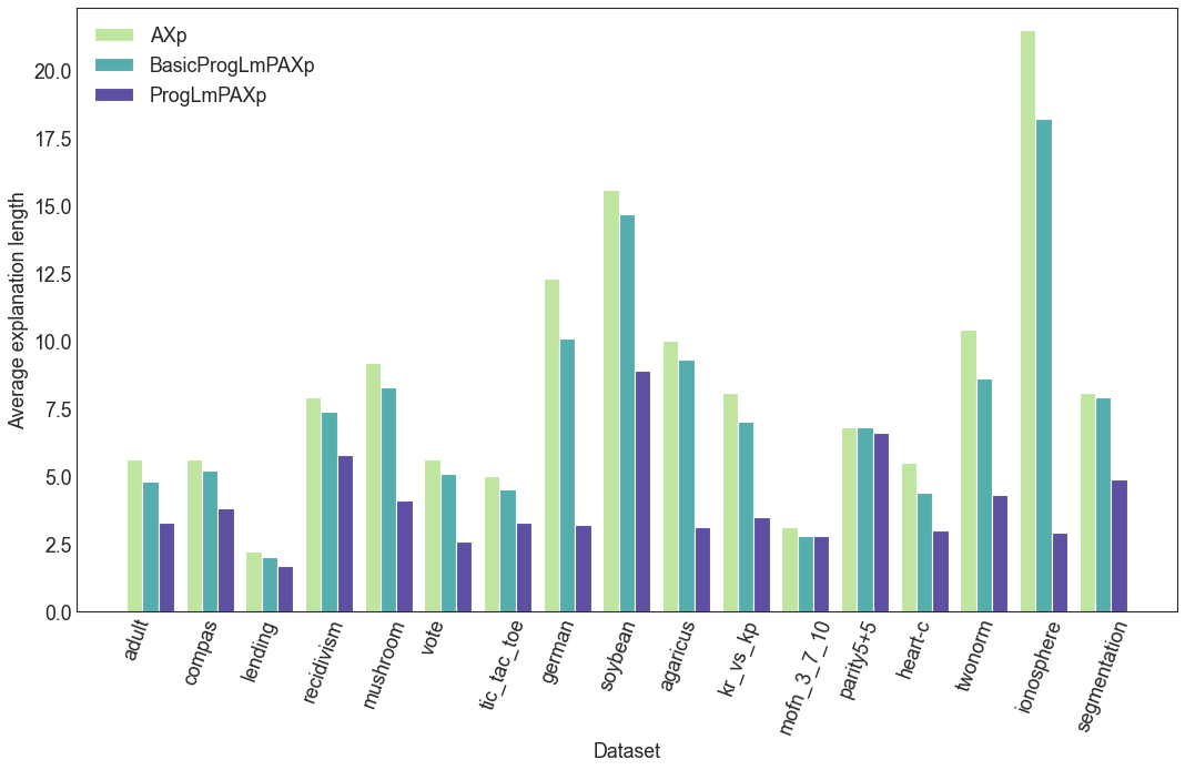
Figure 1: Assessing the gain of probabilistic explanation length compared to abductive explanations for RFs.

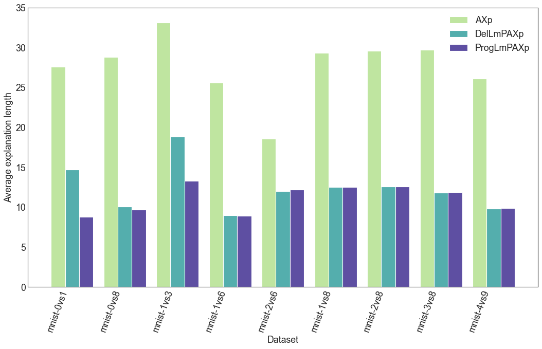
Figure 2: Assessing the gain of probabilistic explanation length compared to abductive explanations for BNNs.

Experimental setup.

The experiments are conducted on Intel Core i5-10500 3.1GHz CPU with 16GByte RAM running Ubuntu 22.04. LTS. A time limit for each single call to the approximate counter is fixed to $120$ seconds and a general time limit for delivering an explanation is set to $600$ seconds; whilst the memory limit is set to 4 GByte.

Benchmarks.

The assessment of RFs is performed on a selection of 17 publicly available datasets, which originate from UCI Machine Learning Repository [UCI,] and Penn Machine Learning Benchmarks [Olson et al., 2017]. Benchmarks comprise binary and multidimensional classification datasets and include binary or/and categorical datasets. (Categorical features are encoded into bit-vectors and handled as a group of attributes representing their original features when computing the explanations.) When training RF classifiers for the selected datasets, we used 80% of the dataset instances (20% used for test data). For assessing explanation tools, we randomly picked fractions of the dataset, depending on the dataset size. Besides, the assessment of BNNs is performed on image datasets of MNIST digits [LeCun et al., 1998]. First, we binarized the data (convert pixel values into 0 or 1) and generated 9 binary class datasets from the original multi-class (from 0 to 9) dataset. Namely, each resulting binary dataset contains images of 2 labels $c_{1}$ versus $c_{2}$ (e.g. mnist-0vs8 comprises samples of class 0 and 8). We considered different tunings of the training parameters so that we obtain the best training and test accuracy of each benchmark.

The precision threshold $\mathrm{T}$ of LmPAXp is fixed to 95% for all considered benchmarks in RFs and 99% for BNN assessment. As results, to guarantee high probabilistic precision of the explanations we implement the approximate model counting metric for BNNs; whilst we apply Monte-Carlo sampling metric for RFs to improve the effectiveness and scalability of our solution. Note that, our observation on preliminary results demonstrate that for $\mathrm{T}\leq 0.97$ both metrics (sampling and model counting) return similar results.

Prototypes implementation.

We developed a reasoner for RFs as a Python script. The script implements the SAT-based approach for explaining RFs proposed by [Izza and Marques-Silva, 2021], in addition the deletion/progression based algorithms described above for computing LmPXAp. Furthermore, PySAT [Ignatiev et al., 2018] is used to instrument incremental SAT oracle calls, and the oracles ApproxMC [Chakraborty et al., 2016, Soos and Meel, 2019, Soos et al., 2020, Meel and Akshay, 2020] and ApproxMCPB [Yang and Meel, 2021, Yang and Meel, 2023] to instrument (approximate) model counting calls on SAT and pseudo-Boolean formulas.

Besides, we reused the BNN encoding of [Jia and Rinard, 2020], cleaned up the source code and implemented both SAT and pseudo-Boolean -based encodings for our formulation of computing explanations. Similarly to RF encoding, we used PySAT to generate BNN SAT-based encoding, and additionally we used the Python package PyPBLib [pypblib, 2023] of PBLib [Philipp and Steinke, 2015], which is integrated in PySAT, to generate the pseudo-Boolean encoding. (Note that PyPBLib/PBLib by design provides efficient clausal form encodings of pseudo-Boolean formulas. Accordingly, we used it on purpose to generate the pseudo-Boolean constraints and convert them into CNF formulas when SAT encoding is selected.) Moreover, Minisat (or Glugose3) SAT solver is instrumented for the resolution of the CNF formulation, whilst pseudo-Boolean oracle Roundingsat [Elffers and Nordström, 2018] is instrumented to solve the pseudo-Boolean encodings. We underline that our observations on preliminary assessments, and also as pointed out in [Jia and Rinard, 2020], pseudo-Boolean encoding and Roundingsat oracle shows (slightly) better performances than SAT oracles. As a result, we solely report the experimental results of the pseudo-Boolean encodings of the selected BNN benchmarks. The implementation of our prototypes is available at https://github.com/izzayacine/praxp.

Results.

Figure 1 and 2 summarize the results of assessing the probabilistic explanation succinctness of RFs and BNNs. Notably, histogram shown Figure 1 reports the average lengths of AXp’s and LmPAXp’s computed with progression algorithm (2) and progression augmented with an heuristic on features contribution in the candidate explanation. (Note that deletion and progression algorithms exhibit similar performances, in terms of explanation lengths and runtimes, on RFs using Monte-Carlo sampling-based approach for approximately counting the models. Thus, results of progression algorithm are solely reported in Figure 1.) As can be observed from Figure 1, with a few exceptions (2 binary datasets out of 17, i.e. mofn_3_7_10 and parity5+5) $\mathsf{LmPAXp}$ provides shorter explanations for all tested datasets and the gap is substantial when activating the heuristic option (reported in ProgLmPAXp in Figure 1) that picks the most likely influent feature at each iteration of the procedure — this is illustrated for example, in ionosphere and german datasets the average size of probabilistic abductive explanations is, resp., 86.6% and 73.9% smaller than plain abductive explanations, with an average precision of 0.97 on all tested samples. Moreover, for the majority of the datasets the average precision is 0.97 or higher, in total 16 out 17 datasets (i.e. 8 out 17, 5 out 17 and 3 out, resp. show an average precision of 0.97, 0.98 and 0.99) and 1 dataset has an average precision of 0.96. Besides, according to our expectations, the average runtimes of our sampling-based approach are small — the minimum average runtime reported is 0.13 seconds, while the maximum does not exceed 4.8 seconds.

The obtained results on BNNs, summarized in Figure 2, show significant size reduction in the explanations of $\mathsf{LmPAXp}$ compared to $\mathsf{AXp}$ while offering a very high probabilistic robustness $\mathrm{T}=0.99$. We observe a difference of average length of 34.5% up to 68.2% between LmPAXp’s and AXp’s, e.g. the average number of pixels for $\mathsf{AXp}$ in mnist-0vs8 is  29, whereas for $\mathsf{LmPAXp}$ it is  10 pixels, which represents 33.6% of its average AXp size. Notice that for BNNs, we compare — as shown in the histogram of Figure 2, the results of deletion and progression algorithms. In fact, one can see from Figure 2 and Table 1 (Runtimes on RFs assessment are reported in the Appendix Table 2) that $\mathsf{ProgLmPAXp}$ returns similar or smaller explanations, and more importantly better runtimes for all BNNs — the average runtimes vary from 63.1 seconds to 114.6 seconds (avg. 79.6 seconds) for $\mathsf{ProgLmPAXp}$ and 27.76 seconds to 460.27 seconds (avg. 196.4 seconds) for $\mathsf{DelLmPAXp}$. This improvement is justified by the effect of applying our heuristic for selecting the next candidate feature during the linear search process, which therefore yields to reduce the number of calls to the model counter oracle when the minimum precision $\mathrm{T}$ is reached. Recall that the number of oracle calls in $\mathsf{DelLmPAXp}$ is fix, in contrast to $\mathsf{ProgLmPAXp}$ where $m$ the number of features to analyze is the upper bound (no matter the applied order of the features). In other hand, we point out that our sampling heuristic helps both methods to get smaller LmPAXp’s than using a simple lexicographical order of the features. Surprisingly, the progression method augmented with the sampling heuristic terminates for all tests in all datasets, while in contrast the deletion method reported timeouts for 3 datasets, in total 138 out of 300 image instances. This demonstrates the scalability of our method implementing progression linear search approach.

Given the above discussion, we can conclude that our solutions for computing locally-minimal formal explanations for complex models that can be encoded into logical formulas, like tree ensembles, binarized neural networks, decision lists, etc, are effective and offer succinct explanations with probabilistic guarantees of precision. Furthermore, depending on the preference of the user to compute robust or high precise probabilistic explanations, we provide two practical solutions: Monte-Carlo sampling-based approach for robust probabilistic explanations and approximate model counting-based approach for tight error tolerance $\epsilon$. Finally, we emphasize the out performance of our $\mathsf{ProgLmPAXp}$ algorithm over $\mathsf{DelLmPAXp}$ in this specific application for searching approximate probabilistic explanations.

Dataset	AXp		DelLmPAXp			ProgLmPAXp
	Len	Time	Len	Time	#TO	Len	Time
mnist-0vs1	$27.6$	$0.81$	$14.7$	$460.27$	$79$	$8.8$	$86.72$
mnist-0vs8	$28.8$	$0.51$	$10.1$	$345.24$	$11$	$9.7$	$85.98$
mnist-1vs3	$33.1$	$0.57$	$18.8$	$284.35$	$48$	$13.3$	$114.63$
mnist-1vs6	$25.6$	$0.52$	$9.0$	$125.69$	$0$	$8.9$	$64.14$
mnist-2vs6	$18.6$	$0.47$	$12.0$	$27.76$	$0$	$12.2$	$43.02$
mnist-1vs8	$29.3$	$0.50$	$12.5$	$150.10$	$0$	$12.5$	$87.71$
mnist-2vs8	$29.6$	$0.48$	$12.6$	$169.04$	$0$	$12.6$	$89.35$
mnist-3vs8	$29.7$	$0.48$	$11.8$	$118.16$	$0$	$11.9$	$81.80$
mnist-4vs9	$26.1$	$0.47$	$9.8$	$87.81$	$0$	$9.9$	$63.14$

Table 1: Detailed performance evaluation of computing locally-minimal PAXp for BNNs trained on (binarized) MNIST datasets. The maximum tolerance is fixed to 0.01, i.e. $\mathrm{T}=0.99$. Columns Len and Time report, resp., the average length of computed AXp’s (resp. LmPAXp) and the average runtime for computing such explanations. Column #TO reports the number timeouts registred over 100 tests for the deletion-based algorithm.

6 Conclusions

Formal explainability witness significant progress in recent years. However, some challenges remain, including the size of explanations. Probabilistic abductive explanations (PAXps) represent a solution to curb explanation size. Unfortunately, their exact computation is impractical. An alternative to PAXps are locally minimal probabilistic abductive explanations (LmPAXps), which recent work showed, for some families of classifiers, that LmPAXps match in practive PAXps. Motivated by these results, this paper proposes two algorithms for approximating the computation of LmPAXps for complex ML models.

The experimental results reveal two possible use-cases, one for each of the proposed algorithms. In application domains where robust explanations suffice, i.e. 90% to 97% precision, the paper proposes a novel algorithm based on MC-sampling, which scales to any classifier. Alternatively, in domains where highly precise explanations are of interest, i.e. around 99% precision, the paper proposes another novel algorithm based on approximate model counting. Besides the counting oracle, this algorithm exploits the use of a geometric progression for searching for features to keep in the explanations, as opposed to using linear search, and shows that the resulting algorithm is more effective in practice.

Future work will consider the use of approximate model counting for families of classifiers beyond boolean domains. This will require integration of approximate model counting with SMT reasoners.

 

Appendix

 

Appendix A SUPPLEMENTARY MATERIAL

A.1 Detailed Results

Dataset	(m, K)		AXp		DelLmPAXp			BasicProgLmPAXp			ProgLmPAXp
			Len	Time	Len	Time	Pr	Len	Time	Pr	Len	Time	Pr
adult	$(12$	$2)$	$5.6$	$0.19$	$3.2$	$0.99$	$0.97$	$4.8$	$0.34$	$0.98$	$3.3$	$0.98$	$0.98$
agaricus_lepiota	$(22$	$2)$	$10.0$	$0.06$	$3.3$	$3.78$	$0.96$	$9.3$	$0.68$	$0.99$	$3.1$	$2.31$	$0.96$
compas	$(11$	$2)$	$5.6$	$0.12$	$3.6$	$0.77$	$0.97$	$5.2$	$0.30$	$0.99$	$3.8$	$0.92$	$0.97$
german	$(21$	$2)$	$12.3$	$0.36$	$3.2$	$5.40$	$0.97$	$10.1$	$0.75$	$0.98$	$3.2$	$2.45$	$0.97$
heart-c	$(13$	$2)$	$5.5$	$0.07$	$3.0$	$0.39$	$0.97$	$4.4$	$0.12$	$0.98$	$3.0$	$0.37$	$0.97$
ionosphere	$(34$	$2)$	$21.5$	$0.06$	$2.9$	$6.59$	$0.96$	$18.2$	$0.51$	$0.97$	$2.9$	$1.58$	$0.97$
kr_vs_kp	$(36$	$2)$	$8.1$	$0.08$	$3.5$	$0.84$	$0.98$	$7.0$	$0.20$	$1.00$	$3.5$	$0.72$	$0.98$
lending	$(9$	$2)$	$2.2$	$0.10$	$1.7$	$0.15$	$0.99$	$2.0$	$0.07$	$0.99$	$1.7$	$0.13$	$0.99$
mofn_3_7_10	$(10$	$2)$	$3.1$	$0.06$	$2.8$	$0.13$	$0.99$	$2.8$	$0.08$	$0.99$	$2.8$	$0.19$	$0.99$
mushroom	$(22$	$2)$	$9.2$	$0.07$	$4.2$	$2.30$	$0.97$	$8.3$	$0.42$	$0.99$	$4.1$	$1.81$	$0.97$
parity5+5	$(10$	$2)$	$6.8$	$0.23$	$6.4$	$0.38$	$1.00$	$6.8$	$0.29$	$1.00$	$6.6$	$0.97$	$0.99$
recidivism	$(15$	$2)$	$7.9$	$0.48$	$5.8$	$1.75$	$0.97$	$7.4$	$0.73$	$0.99$	$5.8$	$2.83$	$0.98$
segmentation	$(19$	$7)$	$8.1$	$0.39$	$4.9$	$0.76$	$0.98$	$7.9$	$0.24$	$0.99$	$4.9$	$0.90$	$0.98$
soybean	$(35$	$18)$	$15.6$	$2.05$	$8.9$	$4.07$	$0.97$	$14.7$	$0.68$	$0.99$	$8.9$	$4.81$	$0.97$
tic_tac_toe	$(9$	$2)$	$5.0$	$0.09$	$3.3$	$0.58$	$0.97$	$4.5$	$0.24$	$0.99$	$3.3$	$0.70$	$0.97$
twonorm	$(20$	$2)$	$10.4$	$0.05$	$4.4$	$1.35$	$0.97$	$8.6$	$0.24$	$0.97$	$4.3$	$1.04$	$0.97$
vote	$(16$	$2)$	$5.6$	$0.07$	$2.6$	$1.16$	$0.98$	$5.1$	$0.32$	$0.99$	$2.6$	$1.02$	$0.98$

Table 2: Detailed performance evaluation of computing LmPAXp for RFs. The table shows results for 17 datasets containing binary and categorical data. The maximum tolerance was fixed to 0.05, i.e. $\mathrm{T}=0.95$. Columns m and K report, respectively, the number of features and classes in the dataset. Columns Len and Time report, resp., the average length of computed AXp’s (resp. LmPAXp) and the average runtime for computing such explanations. Column Pr reports the average precision of the probabilistic explanations.

Dataset	AXp		DelLmPAXp			ProgLmPAXp
	Len	Time	Len	Time	#TO	Len	Time
mnist-0vs1	$27.6$	$0.81$	$14.7$	$460.27$	$79$	$8.8$	$86.72$
mnist-0vs8	$28.8$	$0.51$	$10.1$	$345.24$	$11$	$9.7$	$85.98$
mnist-1vs3	$33.1$	$0.57$	$18.8$	$284.35$	$48$	$13.3$	$114.63$
mnist-1vs6	$25.6$	$0.52$	$9.0$	$125.69$	$0$	$8.9$	$64.14$
mnist-2vs6	$18.6$	$0.47$	$12.0$	$27.76$	$0$	$12.2$	$43.02$
mnist-1vs8	$29.3$	$0.50$	$12.5$	$150.10$	$0$	$12.5$	$87.71$
mnist-2vs8	$29.6$	$0.48$	$12.6$	$169.04$	$0$	$12.6$	$89.35$
mnist-3vs8	$29.7$	$0.48$	$11.8$	$118.16$	$0$	$11.9$	$81.80$
mnist-4vs9	$26.1$	$0.47$	$9.8$	$87.81$	$0$	$9.9$	$63.14$

Table 3: Detailed performance evaluation of computing locally-minimal PAXp for BNNs. The table shows results for 9 binarized MNIST datasets, i.e. each dataset represents class digit $c_{1}$ versus $c_{2}$ (e.g. mnist-4vs9 comprises samples of class 4 and 9). The maximum tolerance is fixed to 0.01, i.e. $\mathrm{T}=0.99$. Columns Len and Time report, resp., the average length of computed AXp’s (resp. LmPAXp) and the average runtime for computing such explanations. Column #TO reports the number timeouts registred over 100 tests for the deletion-based algorithm. Note that progression-based algorithm did not exceed the fixed time limit for all datasets.

References

- [Arenas et al., 2022] Arenas, M., Barceló, P., Romero, M., and Subercaseaux, B. (2022). On computing probabilistic explanations for decision trees. In NeurIPS.
- [Breiman, 2001] Breiman, L. (2001). Random forests. Mach. Learn., 45(1):5–32.
- [Chakraborty et al., 2016] Chakraborty, S., Meel, K. S., and Vardi, M. Y. (2016). Algorithmic improvements in approximate counting for probabilistic inference: From linear to logarithmic SAT calls. In Kambhampati, S., editor, IJCAI, pages 3569–3576. IJCAI/AAAI Press.
- [Cheng et al., 2018] Cheng, C., Nührenberg, G., Huang, C., and Ruess, H. (2018). Verification of binarized neural networks via inter-neuron factoring - (short paper). In Piskac, R. and Rümmer, P., editors, VSTTE, volume 11294 of Lecture Notes in Computer Science, pages 279–290. Springer.
- [Cooper and Marques-Silva, 2021] Cooper, M. C. and Marques-Silva, J. (2021). On the tractability of explaining decisions of classifiers. In Michel, L. D., editor, CP, pages 21:1–21:18.
- [Courbariaux et al., 2016] Courbariaux, M., Hubara, I., Soudry, D., El-Yaniv, R., and Bengio, Y. (2016). Binarized neural networks: Training neural networks with weights and activations constrained to +1 or -1. CoRR, abs/1602.02830.
- [Elffers and Nordström, 2018] Elffers, J. and Nordström, J. (2018). Divide and conquer: Towards faster pseudo-boolean solving. In Lang, J., editor, IJCAI, pages 1291–1299. ijcai.org.
- [Feng and Zhou, 2018] Feng, J. and Zhou, Z. (2018). AutoEncoder by forest. In AAAI, pages 2967–2973.
- [Gao and Zhou, 2020] Gao, W. and Zhou, Z. (2020). Towards convergence rate analysis of random forests for classification. In NeurIPS.
- [Hubara et al., 2016] Hubara, I., Courbariaux, M., Soudry, D., El-Yaniv, R., and Bengio, Y. (2016). Binarized neural networks. In NeurIPS, pages 4107–4115.
- [Ignatiev et al., 2022a] Ignatiev, A., Izza, Y., Stuckey, P., and Marques-Silva, J. (2022a). Using MaxSAT for efficient explanations of tree ensembles. In AAAI.
- [Ignatiev et al., 2022b] Ignatiev, A., Izza, Y., Stuckey, P. J., and Marques-Silva, J. (2022b). Using maxsat for efficient explanations of tree ensembles. In AAAI, pages 3776–3785. AAAI Press.
- [Ignatiev et al., 2018] Ignatiev, A., Morgado, A., and Marques-Silva, J. (2018). PySAT: A python toolkit for prototyping with SAT oracles. In SAT, pages 428–437.
- [Ignatiev et al., 2019] Ignatiev, A., Narodytska, N., and Marques-Silva, J. (2019). Abduction-based explanations for machine learning models. In AAAI, pages 1511–1519.
- [Izza et al., 2023] Izza, Y., Huang, X., Ignatiev, A., Narodytska, N., Cooper, M. C., and Marques-Silva, J. (2023). On computing probabilistic abductive explanations. Int. J. Approx. Reason., 159:108939.
- [Izza and Marques-Silva, 2021] Izza, Y. and Marques-Silva, J. (2021). On explaining random forests with SAT. In IJCAI, pages 2584–2591.
- [Jia and Rinard, 2020] Jia, K. and Rinard, M. C. (2020). Efficient exact verification of binarized neural networks. In NeurIPS.
- [Junker, 2004] Junker, U. (2004). QUICKXPLAIN: preferred explanations and relaxations for over-constrained problems. In AAAI, pages 167–172.
- [Kung et al., 2018] Kung, J., Zhang, D. C., van der Wal, G. S., Chai, S. M., and Mukhopadhyay, S. (2018). Efficient object detection using embedded binarized neural networks. J. Signal Process. Syst., 90(6):877–890.
- [LeCun et al., 1998] LeCun, Y., Bottou, L., Bengio, Y., and Haffner, P. (1998). Gradient-based learning applied to document recognition. Proc. IEEE, 86(11):2278–2324.
- [Marques-Silva and Ignatiev, 2022] Marques-Silva, J. and Ignatiev, A. (2022). Delivering trustworthy AI through formal XAI. In AAAI.
- [Marques-Silva et al., 2013] Marques-Silva, J., Janota, M., and Belov, A. (2013). Minimal sets over monotone predicates in boolean formulae. In CAV, pages 592–607.
- [Marques-Silva et al., 2017] Marques-Silva, J., Janota, M., and Mencía, C. (2017). Minimal sets on propositional formulae. problems and reductions. Artif. Intell., 252:22–50.
- [McDanel et al., 2017] McDanel, B., Teerapittayanon, S., and Kung, H. T. (2017). Embedded binarized neural networks. In EWSN, pages 168–173. Junction Publishing, Canada / ACM.
- [Meel and Akshay, 2020] Meel, K. S. and Akshay, S. (2020). Sparse hashing for scalable approximate model counting: Theory and practice. In LICS, pages 728–741. ACM.
- [Miller, 1956] Miller, G. A. (1956). The magical number seven, plus or minus two: Some limits on our capacity for processing information. Psychological review, 63(2):81–97.
- [Mitzenmacher and Upfal, 2017] Mitzenmacher, M. and Upfal, E. (2017). Probability and Computing: Randomization and Probabilistic Techniques in Algorithms and Data Analysis. Cambridge University Press, USA, 2nd edition.
- [Narodytska et al., 2018] Narodytska, N., Kasiviswanathan, S. P., Ryzhyk, L., Sagiv, M., and Walsh, T. (2018). Verifying properties of binarized deep neural networks. In AAAI, pages 6615–6624.
- [Narodytska et al., 2020] Narodytska, N., Zhang, H., Gupta, A., and Walsh, T. (2020). In search for a SAT-friendly binarized neural network architecture. In ICLR.
- [Olson et al., 2017] Olson, R. S., La Cava, W., Orzechowski, P., Urbanowicz, R. J., and Moore, J. H. (2017). Pmlb: a large benchmark suite for machine learning evaluation and comparison. BioData Mining, 10(36):1–13.
- [Philipp and Steinke, 2015] Philipp, T. and Steinke, P. (2015). Pblib – a library for encoding pseudo-boolean constraints into cnf. In Heule, M. and Weaver, S., editors, SAT, volume 9340, pages 9–16.
- [pypblib, 2023] pypblib (2023). PyPBLib: Python Pseudo-Boolean library. http://ulog.udl.cat/static/doc/pypblib/html/index.html.
- [Shih et al., 2018] Shih, A., Choi, A., and Darwiche, A. (2018). A symbolic approach to explaining bayesian network classifiers. In IJCAI, pages 5103–5111.
- [Sinz, 2005] Sinz, C. (2005). Towards an optimal CNF encoding of boolean cardinality constraints. In van Beek, P., editor, CP, volume 3709 of Lecture Notes in Computer Science, pages 827–831. Springer.
- [Sinz and Dieringer, 2005] Sinz, C. and Dieringer, E. (2005). Dpvis - A tool to visualize the structure of SAT instances. In Bacchus, F. and Walsh, T., editors, SAT, volume 3569, pages 257–268. Springer.
- [Soos et al., 2020] Soos, M., Gocht, S., and Meel, K. S. (2020). Tinted, detached, and lazy CNF-XOR solving and its applications to counting and sampling. In Lahiri, S. K. and Wang, C., editors, CAV, volume 12224, pages 463–484. Springer.
- [Soos and Meel, 2019] Soos, M. and Meel, K. S. (2019). BIRD: engineering an efficient CNF-XOR SAT solver and its applications to approximate model counting. In AAAI, pages 1592–1599. AAAI Press.
- [SoPlex, 2023] SoPlex (2023). Sequential object-oriented simplex. https://soplex.zib.de.
- [UCI, ] UCI. UCI Machine Learning Repository. https://archive.ics.uci.edu/ml.
- [Wäldchen et al., 2021] Wäldchen, S., MacDonald, J., Hauch, S., and Kutyniok, G. (2021). The computational complexity of understanding binary classifier decisions. J. Artif. Intell. Res., 70:351–387.
- [Yang and Meel, 2021] Yang, J. and Meel, K. S. (2021). Engineering an efficient PB-XOR solver. In Michel, L. D., editor, CP, volume 210 of LIPIcs, pages 58:1–58:20.
- [Yang and Meel, 2023] Yang, J. and Meel, K. S. (2023). Rounding meets approximate model counting. In Enea, C. and Lal, A., editors, CAV, volume 13965, pages 132–162. Springer.
- [Yang et al., 2020] Yang, L., Wu, X., Jiang, Y., and Zhou, Z. (2020). Multi-label learning with deep forest. In ECAI, volume 325, pages 1634–1641.
- [Zhang et al., 2019] Zhang, Y., Zhou, J., Zheng, W., Feng, J., Li, L., Liu, Z., Li, M., Zhang, Z., Chen, C., Li, X., Qi, Y. A., and Zhou, Z. (2019). Distributed deep forest and its application to automatic detection of cash-out fraud. ACM Trans. Intell. Syst. Technol., 10(5):55:1–55:19.
- [Zhou and Feng, 2017] Zhou, Z. and Feng, J. (2017). Deep forest: Towards an alternative to deep neural networks. In IJCAI, pages 3553–3559.