Can femtoscopic correlation function shed light on the nature of the lightest, charm, axial mesons?

Abstract

There seem to exist two lightest axial mesons with charm whose masses are very similar but the associated widths and other properties are different. These mesons are denominated as $D_{1}(2430)$ and $D_{1}(2420)$. Although two mesons with similar masses are expected to exist, with such quantum numbers, within the traditional quark model, as we discuss the description of their decay widths and other properties requires contributions from meson-meson coupled channel scattering. We present the amplitudes obtained by solving the Bethe-Salpeter equations which unavoidably lead to the generation of two axial resonances when mesons are considered as the degrees of freedom in the model. One of them is narrow and has properties in good agreement with those of $D_{1}(2420)$. The other pole is wider, but not wide enough to be related to $D_{1}(2430)$. Its position (mass) also does not match well with that of $D_{1}(2430)$. The situation improves when a bare quark-model state is included. Further, we calculate the scattering lengths for different channels and compare them with the available data from lattice QCD. Using arguments of heavy quark symmetry, we discuss possible differences between the scattering lengths coming from the lattice QCD calculations for the $D\pi$ and $D^{*}\pi$ systems and the preliminary experimental data from the ALICE Collaboration on the $D\pi$ system. We present two models, which can produce compatible properties for the two lightest $D_{1}$ states but result in different scattering lengths: one in agreement with the findings of lattice QCD and the other in agreement with the estimation obtained using the $D\pi$ results from the ALICE Collaboration. We present the correlation functions for both cases and discuss how femtoscopic physics can shed light on this issue.

I Introduction

Femtoscopic correlation functions have emerged as a powerful alternative tool to understand the nature of hadrons in recent times (to see the articles published in the current year, for example, see Refs. Acharya et al. (2023a, b, c) or see the review of Ref. Fabbietti et al. (2021)), though the idea is not new Lisa et al. (2005). In the present manuscript, we analyze if the same idea can be implemented to determine the properties of the two lightest $D_{1}$ mesons, $D_{1}(2420)$ and $D_{1}(2430)$, for which the average values of mass and width, as given by the Particle Data Group (PDG) Workman et al. (2022), are:

$$D_{1}(2420): ~{}~{}~{}M=2422.1\pm 0.6\text{ MeV, }\Gamma=31.3\pm 1.9\text{ MeV.}$$

$$D_{1}(2430): ~{}~{}~{}M=2412\pm 9\text{ MeV, }\Gamma=314\pm 29\text{ MeV.}$$ (1)

The evidence for the existence of two $D_{1}$ states, with the aforementioned properties, comes from a fit made to the experimental data on the $D^{*}\pi$ invariant mass distribution Aaij et al. (2015); Abe et al. (2004), where the $S$- and $D$-wave amplitudes are associated with $D_{1}(2430)$ and $D_{1}(2420)$ respectively. From the theory side, the existence of two $c\bar{d}$, $c\bar{u}$ states were predicted, with the spin-parity $J^{\pi}=1^{+}$, in a quark model based on one-gluon-exchange-plus-linear-confinement potential Godfrey and Isgur (1985). Such states were found to arise from the $1^{1}P_{1}$ and $1^{3}P_{1}$ interactions, with masses 2440 MeV and 2490 MeV, respectively, Godfrey and Isgur (1985). An admixture of the states is associated with physical mesons, with a mixing angle of $-41^{0}$ Godfrey and Isgur (1985). Though the masses are not very different from those listed in Eq. (1), the two states would be expected to have similar widths from the point of view of the quark model (as indeed found in Ref. Ferretti and Santopinto (2018), where a width of $\sim 30$ MeV is obtained for both states), thus disagreeing with the experimental findings.

On the other hand, following a different formalism, it was pointed out in Ref. Du et al. (2018) that all the low-lying positive-parity heavy open-flavor mesons can be understood as hadronic molecules. Such claims are motivated by facts like the mass of the lightest open-charm mesons with strangeness are lower than their non-strange counterparts. In Ref. Du et al. (2018), scattering equations were solved using kernels coming from the unitarized chiral perturbation theory for heavy mesons and by fixing the free parameters to fit the scattering lengths determined from Lattice QCD calculations. Within such a framework, two poles were found for $D_{1}$-mesons, with mass, half-width: $2247^{+5}_{-6},~{}107^{+11}_{-10}$ and $2555^{+47}_{-30},~{}203^{+8}_{-9}$ and the lower one was associated with $D_{1}(2430)$. It is argued that the mass value, obtained from a Breit-Wigner fit, given by PDG needs to be revised. A narrow pole, to be associated with $D_{1}(2420)$, however, is not found. Curiously, a very different quark-model calculation Abreu et al. (2019) obtained mass values for the $D_{1}$ states which are very similar to those of Ref. Du et al. (2018). Information on $D_{1}$ mesons is also available from ${}^{2S+1}l_{J}={}^{3}S_{1},~{}{}^{3}D_{1}$ amplitudes determined for the $D^{*}\pi$ system with lattice QCD calculations Lang and Wilson (2022). A broad and a narrow state is found, respectively, in the former and the latter amplitudes. The broad ${}^{3}S_{1}$ state, which is related to $D_{1}(2430)$, has been found to appear at mass 2397 MeV even though the pion mass is larger than the corresponding physical mass, indicating that the pole mass could be lower. Updated calculations, with contributions from channels like $D\pi\pi$, are expected to be determined in future Lang and Wilson (2022), which can shed more light on this topic. As we will discuss, adding coupled channels like $D\rho$ can be important to better determine the properties of the $D_{1}$ states.

Several other attempts have been made to simultaneously describe the properties of the $D_{1}$ states Di Pierro and Eichten (2001); Bardeen et al. (2003); Colangelo et al. (2004); Mehen and Springer (2005); Ni et al. (2022); Kolomeitsev and Lutz (2004); Guo et al. (2007); Gamermann and Oset (2007); Malabarba et al. (2023); Coito et al. (2011); Burns (2014) but there does not seem to arise a consensus on the topic. In such a situation, where a clear manifestation of the states is not seen in the data and relevant information comes from a chi-square fit made to the data, while different models present different results, an alternative tool to test the dispersed findings is needed. We investigate if femtoscopic studies can play such a role.

To carry out such a quest, we extend the framework developed in Refs. Gamermann and Oset (2007); Malabarba et al. (2023) by adding a quark-model pole to the lowest order $D^{*}\pi$ amplitude. We recall that a narrow pole is found to be generated from meson-meson coupled channel dynamics in the former works, which couples mainly to the $D\rho$ channel. The parameters used in Ref. Gamermann and Oset (2007) lead to the formation of such a pole around 2526 MeV. The parameters were fine-tuned in a later work Malabarba et al. (2023) and additional interaction diagrams (box diagrams, based on pion exchange) were added to the lowest order amplitude. As a consequence, a state was found whose mass and width were in excellent agreement with those of $D_{1}(2420)$. It’s worth emphasizing that the aforementioned pole couples strongly to $D\rho$ but very weakly to $D^{*}\pi$, which naturally explains its narrow width that is in contrast with the one of $D_{1}(2430)$. Next we should add that yet another pole, coupling mostly to $D^{*}\pi$, appears in the complex plane in the formalism of Ref. Malabarba et al. (2023), around $2222-i61$ MeV . This latter pole is not in good agreement with the properties of $D_{1}(2430)$. To improve this accordance, we add a bare quark-model pole to the lowest order $D^{*}\pi$ amplitude of Ref. Malabarba et al. (2023).

On solving Bethe-Salpeter equations with such kernels, a broad state, as well as a narrow state, are found in the resulting amplitudes. The narrow state related to $D_{1}(2420)$ is as found in Ref. Malabarba et al. (2023). The broad state has properties closer to those of $D_{1}(2430)$. To further test the reliability of the model we calculate scattering lengths and compare the values for the $D^{*}\pi$ channel with those available from the lattice QCD calculations Mohler et al. (2013) done with a pion mass of 266 MeV. In the former work Mohler et al. (2013), the scattering length for $D\pi$ has also been obtained and a value very similar to the one for $D^{*}\pi$ is found. Such findings can indeed be understood in terms of heavy quark symmetry. In Refs. Liu et al. (2013); Guo et al. (2019), $D\pi$ and other systems are investigated in the lattice QCD formulation, the results of which are used to fix the parameters of the next-to-leading order term of the chiral Lagrangian and the $D\pi$ scattering length is obtained with the physical pion mass. Former values are in agreement with those obtained within unitarized chiral perturbation theory and heavy quark symmetry Guo et al. (2009); Abreu et al. (2011); Geng et al. (2010). Preliminary values for the $D\pi$ scattering length have also been determined by the ALICE Collaboration Alice (see also Refs. Grosa ; Battistini ; Fabbietti et al. ), though, enigmatically, the value determined seems to be different to the results of all the aforementioned works Liu et al. (2013); Guo et al. (2019, 2009); Abreu et al. (2011); Geng et al. (2010). Invoking arguments of heavy quark symmetry, one would expect that the scattering length would be similar for $D^{*}\pi$ and $D\pi$. The question which arises then is if the $D^{*}\pi$ scattering length should be expected to be similar to Refs. Liu et al. (2013); Guo et al. (2019, 2009); Abreu et al. (2011) or Ref. Alice . We contemplate both possibilities in the present manuscript. We find that small changes in the properties of the bare quark-model pole, added to the kernel, can produce a scattering length compatible with the one obtained for $D\pi$ in Refs. Liu et al. (2013); Guo et al. (2019, 2009); Abreu et al. (2011) or with Refs. Alice ; Grosa . Such changes affect the properties of the broader state only while the narrow state remains almost unaltered. Considering both parameterizations we determine the correlation functions for the different coupled systems involved and find that the results for the $D^{*}\pi$ channel are different in the two cases. We present results for different source sizes and discuss if such a tool can be used to decipher the properties of the two lowest-lying $D_{1}$ mesons.

The manuscript is organized as follows. We first discuss the formalism used to determine the amplitudes for different meson-meson systems and present the convention followed to evaluate the scattering length. We give a summary of the scattering lengths obtained within different works, which leads to the consideration of two different parameterizations. We then show the amplitudes, discuss the properties of the resulting poles, and compare the scattering lengths obtained with other works. In a subsequent section, we present the details of the calculations of the correlation function. Finally, we summarize the conclusions of the work.

II Determining the scattering amplitudes

II.1 Formalism to solve the scattering equations

In the present work, we start by following the formalism of Refs. Gamermann and Oset (2007); Malabarba et al. (2023), where nonperturbative interactions between vector and pseudoscalar mesons are considered on the basis of a broken SU(4) symmetry, and add a bare quark-model pole in the kernel. To be more explicit, we begin by considering the lowest order amplitude Gamermann and Oset (2007); Malabarba et al. (2023),

$$t_{ij}=\frac{C_{ij}}{4f^{2}}\left(s-u\right)\vec{\epsilon}\cdot\vec{\epsilon}^{\prime},$$ (2)

where $f$ is the pion decay constant, taken to be 93 MeV, $s$, $u$ are Mandelstam variables, $\epsilon\left(\epsilon^{\prime}\right)$ represents the polarization (three-) vector for the incoming (outgoing) vector meson, and $C_{ij}$ are constants for different $i,~{}j$ (initial, final state).

Though the amplitude in Eq. (2) is obtained in Ref. Gamermann and Oset (2007) by using the SU(4) symmetry, the same can also be determined, as we do, by considering the following Lagrangians Bando et al. (1985, 1988); Meissner (1988); Harada and Yamawaki (2003)

$$\mathcal{L}_{PPV} =-ig_{PPV}\langle V^{\mu}\left[P,~{}\partial_{\mu}P\right]\rangle,$$

$$\mathcal{L}_{VVP} =\frac{g_{VVP}}{\sqrt{2}}\epsilon^{\mu\nu\alpha\beta}\langle\partial_{\mu}V_{\nu}\partial_{\alpha}V_{\beta}P\rangle$$ (3)

to calculate the contribution of a vector-meson exchange in the $t$-channel and by applying the approximation $t\to 0$ at energies near the threshold. We write the SU(4) matrix for pseudoscalar ($P$) and vector ($V$) fields as

$$P =\left(\begin{array}[]{cccc}\frac{\eta}{\sqrt{3}}+\frac{\eta^{\prime}}{\sqrt{6}}+\frac{\pi^{0}}{\sqrt{2}}&\pi^{+}&K^{+}&\bar{D}^{0}\\ \pi^{-}&\frac{\eta}{\sqrt{3}}+\frac{\eta^{\prime}}{\sqrt{6}}-\frac{\pi^{0}}{\sqrt{2}}&K^{0}&D^{-}\\ K^{-}&\bar{K}^{0}&-\frac{\eta}{\sqrt{3}}+\sqrt{\frac{2}{3}}\eta^{\prime}&D^{-}_{s}\\ D^{0}&D^{+}&D_{s}^{+}&\eta_{c}\end{array}\right),$$ (8)

$$V_{\mu} =\left(\begin{array}[]{cccc}\frac{\omega}{\sqrt{2}}+\frac{\rho^{0}}{\sqrt{2}}&\rho^{+}&K^{*+}&\bar{D}^{*0}\\ \rho^{-}&\frac{\omega}{\sqrt{2}}-\frac{\rho^{0}}{\sqrt{2}}&K^{*0}&D^{*-}\\ K^{*-}&\bar{K}^{*0}&\phi&D^{*-}_{s}\\ D^{*0}&D^{*+}&D_{s}^{*+}&J/\Psi\end{array}\right),$$ (13)

which are slightly different from those in Refs. Gamermann and Oset (2007); Malabarba et al. (2023). The difference arises from including the mixing between $\eta-\eta^{\prime}-\eta_{c}$ and $\omega-\phi-J/\Psi$, which gives slightly different amplitudes. We, thus, provide the values of $C_{ij}$ in Table 1.

Table 1: Values of the $C_{ij}$ constants appearing in Eq. (2) for different processes in the isospin 1/2 configuration. Here $\gamma=\left(\frac{m_{L}}{m_{H}}\right)^{2}$, where $m_{L}=800$ MeV and $m_{H}=2050$ MeV are average masses of the light and heavy vector-mesons, as defined in Refs. Gamermann and Oset (2007). In the case of isospin 3/2, we have two channels: $D^{*}\pi$ and $D\rho$ with the diagonal values of $C_{ij}$ being 1 and the non-diagonal being $\gamma$.

	$\pi D^{*}$	$D\rho$	$\bar{K}D_{s}^{*}$	$D_{s}\bar{K}^{*}$	$\eta D^{*}$	$D\omega$	$\eta_{c}D^{*}$	$DJ\Psi$	$D\phi$	$\eta^{\prime}D^{*}$
$\pi D^{*}$	$-2$	$\gamma/2$	$-\sqrt{\frac{3}{2}}$	0	0	$\frac{\sqrt{3}\gamma}{2}$	0	$-\sqrt{\frac{3}{2}}\gamma$	0	0
$D\rho$		$-2$	0	$\sqrt{\frac{3}{2}}$	$-\sqrt{\frac{1}{2}}\gamma$	0	$\sqrt{\frac{3}{2}}\gamma$	0	0	$-\frac{\gamma}{2}$
$\bar{K}D_{s}^{*}$			$-1$	0	$-\frac{2}{\sqrt{3}}$	0	0	$-\gamma$	$\gamma$	$\frac{1}{\sqrt{6}}$
$D_{s}\bar{K}^{*}$				$-1$	$-\frac{\gamma}{\sqrt{3}}$	$-\frac{1}{\sqrt{2}}$	$-\gamma$	0	1	$\sqrt{\frac{2}{3}}\gamma$
$\eta D^{*}$					0	$\frac{\gamma}{\sqrt{6}}$	0	$-\frac{\gamma}{\sqrt{3}}$	0	0
$D\omega$						0	$-\frac{\gamma}{\sqrt{2}}$	0	0	$\frac{\gamma}{2\sqrt{3}}$
$\eta_{c}D^{*}$							0	$\gamma$	0	0
$DJ\Psi$								0	0	$-\frac{\gamma}{\sqrt{6}}$
$D\phi$									0	0
$\eta^{\prime}D^{*}$										0

Besides Eq. (2), we consider contributions coming from a pseudoscalar exchange through box diagrams as obtained in Ref. Malabarba et al. (2023) for the $D\rho\to D^{*}\pi\to D\rho$. If we solve the Bethe-Salpeter equation

$$T=V+VGT,$$ (14)

with such amplitudes, just as done in Ref. Malabarba et al. (2023), we find results very similar to those of Ref. Malabarba et al. (2023). Thus, as expected, the mixing between $\eta-\eta^{\prime}-\eta_{c}$ and $\omega-\phi-J/\Psi$ do not give important contributions.

The loop function, $G$, in Eq. (14), for the $k$th channel, is Gamermann and Oset (2007); Malabarba et al. (2023)

$$G_{k}\left(\sqrt{s}\right)=\int\frac{d^{4}q}{\left(2\pi\right)^{4}}\frac{1}{\left(P-q\right)^{2}-M^{2}_{k}}\frac{1}{q^{2}-m_{k}^{2}}$$

$$=\frac{1}{16\pi^{2}}\Biggl{[}a_{k}\left(\mu\right)+\ln{\frac{m_{k}^{2}}{\mu^{2}}}+\frac{M_{k}^{2}-m_{k}^{2}+s}{2s}\ln{\frac{M_{k}^{2}}{m_{k}^{2}}}+\frac{q_{k}}{\sqrt{s}}\Biggl{(}\ln{\frac{s-\left(M_{k}^{2}-m_{k}^{2}\right)+2q_{k}\sqrt{s}}{-s+\left(M_{k}^{2}-m_{k}^{2}\right)+2q_{k}\sqrt{s}}}\Biggr{.}\Biggr{.}$$

$$+\Biggl{.}\Biggl{.}\ln{\frac{s+\left(M_{k}^{2}-m_{k}^{2}\right)+2q_{k}\sqrt{s}}{-s-\left(M_{k}^{2}-m_{k}^{2}\right)+2q_{k}\sqrt{s}}}\Biggr{)}\Biggr{]}\left(1+\frac{q_{k}^{2}}{3M_{k}^{2}}\right),$$ (15)

with $P$ representing the total four-momentum of the system and $q$ the four-momentum of one of the mesons, $M_{k}$ ($m_{k}$) standing for the mass of the vector (pseudoscalar) meson in the $k$th channel, $a_{k}$ and $\mu$ denoting a subtraction constant needed to regularize the divergent nature of the $G$-function and the regularization scale respectively. The values for the regularization parameters are taken to be Malabarba et al. (2023) $\mu=1500$, $a=-1.45$, and we consider the convolution of $G$-function over the finite widths of $\rho$ and $K^{*}$. The resulting amplitudes show the presence of a state with mass $~{}\sim 2428$ MeV and width $\sim 33$ MeV on the real axis, as in Ref. Malabarba et al. (2023). This latter state couples strongly to the $D\rho$ channel and weakly to the $D^{*}\pi$ channel, and its properties are in excellent agreement with those of $D_{1}(2420)$. There appears another pole at $2220-i61$ MeV, which couples mostly to $D^{*}\pi$ but which cannot be related to $D_{1}(2430)$ (see Fig. 1).

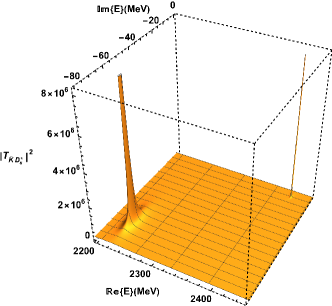
Figure 1: Two poles appearing in the $\bar{K}D_{s}^{*}$ amplitude. While the narrower pole can be associated with $D_{1}(2420)$, the broader pole does not represent the properties of $D_{1}(2430)$. It should be mentioned that here we have chosen to show the $\bar{K}D_{s}^{*}$ amplitude as an example. The poles are seen in all the coupled channels, as the case should be.

Notice that the half-width of the narrow pole is around 5 MeV, in the complex plane, but the width on the real axis becomes 33 MeV on consideration of the finite widths of the $\rho$ and $K^{*}$ mesons. The width of the lower energy pole also increases, to  130 MeV, but still remains too small for the purpose of its association with $D_{1}(2430)$. Besides the mass also remains too low. We show the $D^{*}\pi$ and $D\rho$ squared amplitudes, on the real axis, as solid lines in Fig. 2.

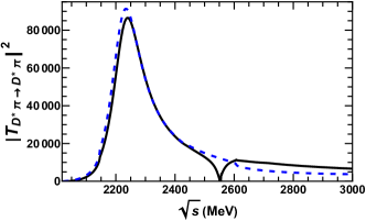
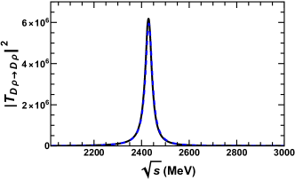
Figure 2: Projection of the poles shown in Fig. 1 on the real axis, shown by depicting the squared amplitudes for the $D^{*}\pi$ and $D\rho$ channels. The solid lines are the results of solving the scattering equation with ten coupled channels (given in Table 1), while the dashed lines result from considering only the first four channels, which are $D^{*}\pi$, $D\rho$, $\bar{K}D^{*}_{s}$ and $D_{s}\bar{K}^{*}$. The two results look very similar, except for a $\eta D^{*}$ cusp effect seen around 2556 MeV in the $D^{*}\pi$ amplitude, shown as a solid line.

The results shown as dashed lines, Fig. 2, correspond to those obtained by considering only the first four channels of Table 1. It can be seen the results are almost unchanged, indicating that the most relevant channels to study the mentioned $D_{1}$ states are $D^{*}\pi$, $D\rho$, $\bar{K}D^{*}_{s}$ and $D_{s}\bar{K}^{*}$. The non-compatibility between the properties of $D_{1}(2430)$ and the lower energy pole seen in Fig. 1, whose effect on the real axis is shown in the left panel of Fig. 2, shows that something is missing in the model. We must recall at this point that the degrees of freedom considered in our model, so far, are hadrons and other inputs could be necessary to better describe the properties of $D_{1}(2420)$ and $D_{1}(2430)$ simultaneously.

For this purpose, as a next step, we try adding a bare quark-model pole to the lowest order amplitude for the $D^{*}\pi$ channel

$$V_{QM}=\pm\frac{g^{2}_{QM}}{s-M_{QM}^{2}},$$ (16)

where the mass, $M_{QM}$, can be taken from different quark model calculations Godfrey and Isgur (1985); Ferretti and Santopinto (2018); Abreu et al. (2019) and $g_{QM}$ can be adjusted to obtain a better agreement between the lower energy pole shown in Fig. 1 and the properties of $D_{1}(2430)$. The resulting lowest order amplitude for $D^{*}\pi$ is then the sum of diagrams shown in Fig. 3.

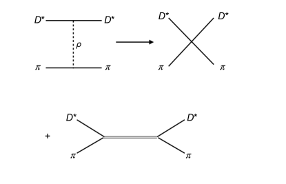
Figure 3: Lowest order amplitude for the $D^{*}\pi$ channel. The upper diagram originates from a vector exchange in the $t$-channel, whereas the lower one arises from the exchange of a bare quark-model pole in the $s$-channel.

As we shall show next, the ansatz works well, and considering values of $M_{QM}$ from Refs. Godfrey and Isgur (1985); Ferretti and Santopinto (2018); Abreu et al. (2019) leads to the appearance of two poles in the amplitudes whose properties are in good accordance with the $D_{1}$ states of interest. The quark-model pole moves in the complex plane, as a consequence of non-perturbative meson-meson interactions, and becomes virtual, while the lower energy pole shown in Fig. 1 attains a larger mass and width. The reflection of such a pole shows properties in agreement with that of $D_{1}(2430)$.

II.2 Scattering lengths and related uncertainties

Before depicting the amplitudes for different channels, we digress a bit towards the discussion of another observable, on which information is available from different sources. The observable being referred to is the scattering length, which we calculate for different channels through the relation

$$a_{i}=\frac{T_{ii}}{8\pi\sqrt{s}}.$$ (17)

We compare the results for the $D^{*}\pi$ channel with the information available from lattice QCD calculations Mohler et al. (2013). The former work determined the isospin 1/2 scattering lengths for $D\pi$ and $D^{*}\pi$ channels and obtained the following values:

$$a^{(1/2)}_{D\pi} =0.81\pm 0.14\text{ fm,}$$

$$a^{(1/2)}_{D^{*}\pi} =0.81\pm 0.17\text{ fm,}$$ (18)

at a pion mass of 266 MeV. As can be seen, the values for the two channels are very similar. Such a finding can be understood by invoking arguments of heavy quark symmetry. It is important to stress here that a sign convention opposite to that given in Eq. (17) is followed in Ref. Mohler et al. (2013). Further, scattering lengths for systems like $D\bar{K}$, $D_{s}\pi$, $D_{s}K$ and $D\pi$ in isospin 3/2 configurations have been obtained on a lattice in Ref. Liu et al. (2013). Using the values of the low energy constants of the chiral Lagrangian fixed from such a study, the scattering length for $D\pi$ in isospin 1/2 is determined. The results from the former works, obtained at the physical pion mass, can be summarized as

$$a^{(1/2)}_{D\pi} =0.37\pm 0.01\text{ fm,}$$

$$a^{(3/2)}_{D\pi} =-0.100(1)\text{ fm.}$$ (19)

It is worth mentioning here that the value of $a^{(1/2)}_{D\pi}$ at $m_{\pi}=266$ MeV is obtained to be $2.30^{+2.40}_{-0.66}$ fm in Ref. Liu et al. (2013), which is higher than that of Ref. Mohler et al. (2013) [given in Eq. (18)]. On the other hand, results compatible with Eq. (19) have been obtained in Refs. Guo et al. (2019, 2009), by using effective theories based on chiral and heavy quark symmetry and by constraining the values of the unknown parameters to fit the results available from lattice QCD. Somewhat smaller values for the isospin 1/2, around 0.2 fm, are found in Refs. Abreu et al. (2011); Geng et al. (2010), which are compatible with the results obtained using the leading order term of the chiral effective Lagrangian Guo et al. (2019, 2009).

Preliminary results on the $D\pi$ scattering length are available from an alternative source, from the Alice Collaboration Alice ; Grosa , which seem to be in disagreement with the aforementioned values. Let us denote the values given in Refs. Alice ; Grosa as $\tilde{a}^{(I)}$. Using such a notation, the values in Refs. Alice ; Grosa can be summarized as

$$\tilde{a}^{(1/2)}_{D\pi} =-0.14\text{ fm to }0.08\text{ fm},$$

$$\tilde{a}^{(3/2)}_{D^{\pi}} =-0.15\text{ fm to }0.01\text{ fm}.$$ (20)

We can expect that $D^{*}\pi$ scattering length would be similar to that for $D\pi$. However, it is not clear which of the two sets of values in Eqs. (19) and (20) should be considered as a benchmark. We find it instructive to investigate both possibilities. In the following discussions, we show that small changes in the value of the mass of the quark-model pole lead to scattering length values compatible with Eq. (19) or (20), though the properties of the two $D_{1}$ states appearing in the amplitudes remain compatible with those of the known states.

II.3 Amplitudes: Results and discussions

As mentioned in the preceding discussions, we add Eq. (16) to the amplitudes already considered in Refs. Gamermann and Oset (2007); Malabarba et al. (2023) with the idea of having the presence of a wide as well as a narrow $D_{1}$ state around 2430 MeV. In addition for the amplitudes to show states with properties compatible with those of $D_{1}(2420)$ and $D_{1}(2430)$, we require the values of the $D^{*}\pi$ scattering lengths to be in agreement with Eq. (19) or (20). For this purpose, we shall consider two different sets of values for the parameters $M_{QM}$ and $g_{QM}$, and refer to the cases as models A and B. It must be clarified here that there is little room for changing the only other possible parameter of the model, which is the subtraction constant used to regularize the loop function, since the properties of $D_{1}(2420)$ are well described by our amplitudes as discussed in Ref. Malabarba et al. (2023). Note that the scale $\mu$ and the subtraction constant $a_{k}$ appearing in Eq. (15) are not two parameters. Both are related to each other and, hence, together they account for one parameter only.

It should be emphasized that adding the bare pole to the $D^{*}\pi$ amplitude does not affect the narrow pole associated with $D_{1}(2420)$ and only the wider pole changes its position in the complex plane. The ansatz followed in the work, as summarized in Fig 3, is chosen on purpose since a good description of $D_{1}(2420)$ is already obtained with the meson degrees of freedom. The added quark-model pole, on the other hand, in the two models discussed subsequently, becomes a virtual pole  and does not leave any trace on the real axis in one of the cases.

II.3.1 Model A

One of the choices we make is to write Eq. (16) as

$$V_{QM}=-\frac{6000^{2}}{s-2440^{2}},$$ (21)

where the value of the mass, $M_{QM}=2440$ MeV, is taken from the quark model of Ref. Godfrey and Isgur (1985). Such a choice, together with $g_{QM}=6000$ MeV, leads the lower energy pole in Fig. 1 to move to $E-i\Gamma/2=2268-i100$ MeV. We stress that we solve the Bethe-Salpeter equation by considering the first four channels shown in Table 1. As already shown in Fig. 2, the first four channels of Table 1 are found to be the most relevant ones for studying $D_{1}$ states in the energy region of 2150-3000 MeV.

The narrow pole, shown in Fig. 1, remains almost unchanged and the bare quark-model pole becomes a virtual one. The wider pole, obtained at $E-i\Gamma/2=2268-i100$, coincides with the lowest $D_{1}$ state found in unitarized chiral perturbation calculations Du et al. (2018) where the free parameters of the next-leading-order term have been fixed by using lattice QCD calculations. The results of Refs. Abreu et al. (2019); Di Pierro and Eichten (2001) also agree with Ref. Du et al. (2018). Let us discuss the effect of the choice of parameters, together with the negative sign, shown in Eq. (21), on the real axis. For this, we show the squared amplitudes for the different channels in Fig. 4.

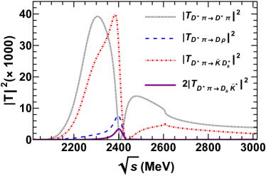
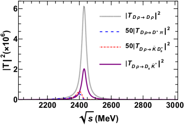
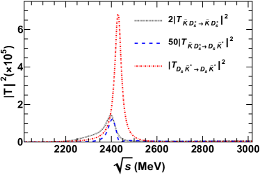
Figure 4: Squared amplitudes of different processes. A factor written in front of $|T_{...}|^{2}$, in the legends, implies that it has been multiplied to the squared matrix such that different amplitudes can be seen in the same scale.

As can be seen in the left panel of the top row of Fig. 4, the $D^{*}\pi$ amplitude shows a peak on the real axis around 2304 MeV, with a full width at half maximum of around 160 MeV. Such a width is more in agreement with the lower limit determined by the Babar Collaboration Aubert et al. (2006). The same amplitude shows a zero near 2400 MeV, which is an effect of the negative interference between the lower energy pole arising from meson-meson dynamics and the quark-model pole. Further, it can be seen that the $D\rho$ amplitude is almost the same in Fig. 2 and 4. Thus, clearly, the $D^{*}\pi$ amplitude is dominated by the wider $D_{1}$ state and does not show any clear sign of $D_{1}(2420)$, while the $D\rho$ amplitude shows only the presence of the narrow pole. In fact we find that the $D^{*}\pi$ amplitude gets very little contribution from the coupled channel interactions. Some of the transition amplitudes, like $D^{*}\pi\to D\rho$, do show the presence of an interference effect between a bump and a narrow peak. Such findings are in consonance with the couplings found for the two $D_{1}$ states to the different channels, as listed in Table 2. These couplings have been determined by calculating the residues of the $t$-matrices in the complex energy plane.

We find it relevant to provide the values of the scattering length for different channels also (see Table 2). As discussed earlier, the value for $D^{*}\pi$ is especially interesting since it can be related to the information available on the $D\pi$ channel. We find a value that is in line with the $D\pi$ scattering lengths determined by effective theories [given in Eq. (19)].

Table 2: Values of the isospin 1/2 scattering lengths and the couplings, represented as $g$, of the two states $D_{1}$ for the different channels.

	$a^{(1/2)}$	$g_{D_{1}(2430)}$	$g_{D_{1}(2420)}$
	(fm)	(MeV)	(MeV)
$D^{*}\pi$	$-0.20$	$7250-i4995$	$-233+i5$
$D\rho$	$0.44-i0.18$	$-521-i355$	$15144+i356$
$\bar{K}D_{s}^{*}$	$0.00-i0.12$	$4534-i3612$	$-247-i177$
$D_{s}\bar{K}^{*}$	$0.00-i0.12$	$2-i55$	$-8739+i90$

II.3.2 Model B

Contrary to Model A, where the mass of a bare pole is taken from a quark model and the coupling, as well as the sign, are chosen so as to determine a pole consistent with Refs. Du et al. (2018); Abreu et al. (2019); Di Pierro and Eichten (2001), we now consider the parameters of Eq. (16) as free. We allow them to vary such as to move the lower energy pole shown in Fig. 1 deeper in the complex plane, thus, providing the possibility of associating a bigger width to the state to be related to $D_{1}(2430)$. As a result, we obtain the following parameterization

$$V_{QM}=\frac{10000^{2}}{s-2370^{2}}.$$ (22)

The precise position of the pole related to $D_{1}(2430)$ is found to be $2218-i218$ MeV. In this case, a broad bump is found on the real axis around 2436 MeV with a full width at half maximum being $\sim$ 311 MeV (see Fig. 5).

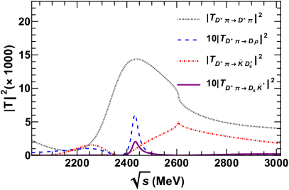
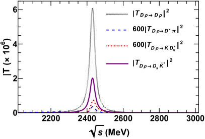
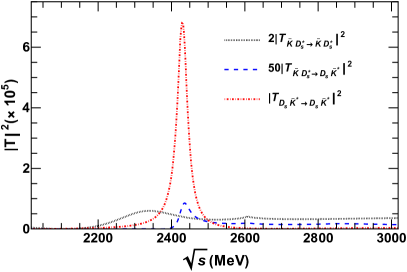
Figure 5: Same as in Fig. 4 but for the parameter choice B shown in Eq. (22.

This covers the possibility of a positive interference between the pole arising from the meson-meson dynamics and the bare quark model pole which becomes a virtual pole when the scattering equation is solved. The resulting mass and width values are more in agreement with those found by the LHCb and Belle Collaborations Aaij et al. (2015); Abe et al. (2004) [as also given in Eq. (1)]. Before continuing with further discussions, we must add here that the values of the parameters in Eq. (22) could be changed a bit which would lead to the mass and width still being in agreement with those of $D_{1}(2430)$. Such changes could provide some uncertainty in the amplitudes, but we take here the values of the parameters in Eq. (22) as an example leading to a scenario compatible with the experimental information.

It can be also noticed that the $D\rho\to D\rho$ as well as $D\rho\to D_{s}\bar{K}^{*}$ amplitudes are almost the same as obtained in model A (see Fig. 4), though the strength of the transition of $D\rho$ to the other two channels has diminished. Besides such changes, a cusp effect is seen near 2607 MeV, especially in $D^{*}\pi\to D^{*}\pi$ as well as $D^{*}\pi\to\bar{K}D_{s}^{*}$, which corresponds to the opening of the $\bar{K}D_{s}^{*}$ channel. We must also mention that the $D^{*}\pi$ amplitude, as mentioned in the discussions of model A, gets little contribution from the coupled channel interactions.

In this case, as shown in Table 3, the scattering length of $D^{*}\pi$ turns out to be more in agreement with the value for $D\pi$ determined by the Alice Collaboration [given in Eq. (20)]. We provide the couplings of the two states to the different channels too in Table 3.

Table 3: Values of the isospin 1/2 scattering lengths and the couplings, represented as $g$, of the two states $D_{1}$ for the different channels.

	$a^{(1/2)}$	$g_{D_{1}(2430)}$	$g_{D_{1}(2420)}$
	(fm)	(MeV)	(MeV)
$D^{*}\pi$	$0.1$	$5199-i3577$	$92-i105$
$D\rho$	$0.45-i0.18$	$-248-i91$	$14987+i232$
$\bar{K}D_{s}^{*}$	$0.00-i0.12$	$3806-i2249$	$186-i39$
$D_{s}\bar{K}^{*}$	$0.00-i0.12$	$-34-i36$	$-8668+i151$

To summarize this section, we can say that we have studied the interactions of different meson-meson systems coupling to the quantum numbers of $D_{1}$ states. We find that, within the model considered, the meson-meson interactions can well describe the properties of $D_{1}(2420)$. A wider pole at lower energies is also generated from the interactions, though the mass and width are not found to be in good agreement with the known properties of $D_{1}(2430)$. We find that adding a bare quark model pole to the $D^{*}\pi$ amplitude improves the situation. We present two scenarios, which lead to values of $D^{*}\pi$ scattering length in agreement with the conflicting ones known for $D\pi$ from lattice QCD-inspired models and from the Alice Collaboration. We now study how such scenarios reflect in terms of the correlation functions. To calculate correlation functions in particle basis, we require the amplitudes in the isospin 3/2 basis too. We end this section by showing such amplitudes in Fig. 6.

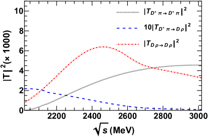
Figure 6: Squared amplitudes for the different channels in the isospin 3/2 basis. These amplitudes have been obtained by using Eq. (2) with the values of $C_{ij}$ given in the caption of Table 1.

Notice that the interactions are weakly repulsive in this isospin configuration and, thus, no states are formed in this case. The scattering lengths in this case are $a_{D^{*}\pi}^{(3/2)}=0.1$ fm and $a_{D\rho}^{(3/2)}=0.2$ fm. The value of the isospin 3/2 scattering length, for the $D^{*}\pi$ channel, is in agreement with the one determined for $D\pi$ in other works [as summarized in Eqs. (19) and (20)]. We remind the reader that the our sign convention (as given in section II.2) is opposite to the one followed in the works leading to the values of Eqs. (19) and (20).

III Correlation Functions

III.1 Formalism

The femtoscopic analysis is based on the estimation of the correlation functions (CFs). A two-particle correlation function is constructed as the ratio of the probability of measuring the two-particle state and the product of the probabilities of measuring each individual particle Lisa et al. (2005). A convenient form relating the correlation function to the source function by means of a convolution with the relative two-particle wave function $\Psi$ is written, after certain approximations, as Lisa et al. (2005); Koonin (1977); Pratt (1986); Lednicky and Lyuboshits (1981); Lednicky et al. (1998)

$$C(k) = \int d^{3}rS_{12}(\vec{r})|\Psi(\vec{k};\vec{r})|^{2},$$ (23)

where $\vec{k}$ is the relative momentum in the center of mass (CM) of the pair; $\vec{r}$ is the relative distance between the two particles; and $S_{12}(\vec{r})$ is the normalized source function, $\int d^{3}rS_{12}(\vec{r})=1$, describing the distribution of relative positions of particles with identical velocities as they move in their asymptotic state (for a detailed discussion see for example Ref. Lisa et al. (2005)). As a consequence, the expression above for $C(k)$ encodes information on both the hadron source and the hadron-hadron interactions and is commonly named as Koonin–Pratt equation Koonin (1977); Pratt (1986) .

In the present work, we employ a source function parametrized as a static Gaussian normalized to unity, i.e.

$$S_{12}(\vec{r}) = \frac{1}{\left(4\pi\right)^{\frac{3}{2}}R^{3}}\exp{\left(-\frac{r^{2}}{4R^{2}}\right)},$$ (24)

where $R$ is the source size parameter. As discussed in Ref. Lisa et al. (2005), Gaussian parametrizations provide an acceptable minimal description of data in a much more simpler way than others with non-Gaussian aspects of the correlation, such as the ones based on the decomposition in spherical or Cartesian harmonics. Thus, the source function in Eq. (24) can be seen as the appropriate parametrization for the sake of its functionality.

To connect the CF to the coupled-channel approach described in the previous section, we adopt the framework summarized in Refs. Vidana et al. (2023); Feijoo et al. (2023); Albaladejo et al. (2023), in which the generalized coupled-channel CF for a specific channel $i$ reads

$$C_{i}(k) = 1+4\pi\theta(q_{max}-k)\int_{0}^{\infty}drr^{2}S_{12}(\vec{r})\left(\sum_{j}w_{j}|j_{0}(kr)\delta_{ji}+T_{ji}(\sqrt{s})\widetilde{G}_{j}(r;s)|^{2}-j_{0}^{2}(kr)\right),$$

where $w_{j}$ is the weight of the observed channel $j$ (we use $w_{j}=1$); $j_{\nu}(kr)$ is the spherical Bessel function; $E=\sqrt{s}$ is the CM energy; the relative momentum of the channel is $k=\lambda^{1/2}(s,m_{1}^{2},m_{2}^{2})/(2\sqrt{s})$ ($\lambda$ being the Källen function and $m_{1},m_{2}$ the masses of the mesons in the channel $i$); $T_{ji}$ are the elements of the scattering matrix encoding the meson–meson interactions, obtained and analyzed in the previous section; and the $\widetilde{G}_{j}(r;s)$ function is defined as

$$\widetilde{G}_{j}(r;s) = \int_{|\vec{q}|<q_{max}}\frac{d^{3}q}{(2\pi)^{3}}\frac{\omega_{1}^{(j)}+\omega_{2}^{(j)}}{2\omega_{1}^{(j)}\omega_{2}^{(j)}}\frac{j_{0}(qr)}{s-\left(\omega_{1}^{(j)}+\omega_{2}^{(j)}\right)^{2}+i\varepsilon},$$ (26)

with $\omega_{a}^{(j)}\equiv\omega_{a}^{(j)}(k)=\sqrt{k^{2}+m_{a}^{2}}$ being the energy of the particle $a$, and $q_{max}$ being a sharp cutoff momentum introduced to regularize the $r\to 0$ behavior. We choose a value for $q_{max}$ within its natural range ($[600,900]\ \mathrm{MeV}$): $q_{max}=700\ \mathrm{MeV}$. We remark that the results for the CFs remain almost the same for different values of $q_{max}$ within the mentioned range, as expected because of the presence of $j_{0}(qr)$ in the integrand, which prevents sizable changes for large values of $q$.

III.2 Lednicky-Lyuboshits approximation

To shed some light on the interpretation of the CFs, it can be instructive to review the Lednicky-Lyuboshits (LL) model, which is based on replacing the full wave function for a single channel by its non-relativistic, asymptotic ($r\to\infty$) form, corresponding to the superposition of plane and converging spherical waves Lednicky and Lyuboshits (1981). In particular, we benefit from the discussion presented in the Appendix of Ref. Albaladejo et al. (2023) and Sections V.B and V.C of Ref. Kamiya et al. (2022), which have some of their fundamental aspects reproduced here.

Proceeding ahead, the consideration of the LL approximation, together with a Gaussian source, and using the relationship between the standard quantum mechanics amplitude $f(k)$ and the scattering matrix $T$, i.e. $f(k)=-T/(8\pi\sqrt{s})$, allow us to write the single-channel CF as Fabbietti et al. (2021); Lednicky and Lyuboshits (1981); Kamiya et al. (2022); Albaladejo et al. (2023)

$$C_{LL}(k) = 1+\frac{|T|^{2}}{2R^{2}(8\pi\sqrt{s})^{2}}F_{1}\left(\frac{r_{eff}}{R}\right)-\frac{2Re[T]}{8\pi^{3/2}R\sqrt{s}}F_{2}(2kR)+\frac{Im[T]}{R\sqrt{s}}F_{3}(2kR),$$ (27)

where $F_{1}(z)=1-z/(2\sqrt{\pi})$, $F_{2}(z)=\int_{0}^{z}dte^{t^{2}-z^{2}}/z$ and $F_{3}(z)=(1-e^{-z^{2}})/z$; $r_{eff}$ is the effective range. An alternative version of Eq. (27) can be obtained by employing the formula 

$$-\frac{T}{8\pi\sqrt{s}}\equiv\frac{1}{k\cot{\delta(k)}-ik}=\frac{R}{-R/a-ikR},$$ (28)

where $r_{eff}$ is taken as zero.

In this way Eq. (27) becomes Kamiya et al. (2022); Albaladejo et al. (2023)

$$C_{LL}(x,y) = 1+\frac{1}{x^{2}+y^{2}}\left[\frac{1}{2}-\frac{2y}{\sqrt{\pi}}F_{2}(2x)-xF_{3}(2x)\right],$$ (29)

where $x=kR$ and $y=R/a$. In the low-momentum limit $(x\to 0)$ we have $F_{2}\to 1$ and $F_{3}\to 0$, which yields

$$C_{LL}(x,y) \overset{x\rightarrow 0}{\longrightarrow} 1-\frac{2}{\pi}+\frac{1}{2}\left(\frac{1}{y}-\frac{2}{\sqrt{\pi}}\right)^{2}$$ (30)

$$= 1-\frac{2}{\sqrt{\pi}}\left(\frac{a}{R}\right)+\frac{1}{2}\left(\frac{a}{R}\right)^{2}.$$

Thus, considering an attractive interaction generated by the strong force, the CF given in Eqs. (29) and (30) behaves as follows. Near the threshold, for negative values of the scattering length (which means an unbound scenario for the system) the CF acquires (i) a strong enhancement when $|a|\gg R$ (i.e. smaller source); (ii) a moderate enhancement when $|a|\sim R$; and (iii) a value $C_{LL}(0)\gtrsim 1$ when $|a|\ll R$ (larger source). On the other hand, in the situation of $a>0$, corresponding to an attractive interaction which could generate a bound or quasi-bound state, in the low-momentum limit, the CF achieves (i) a strong enhancement for smaller sources $(a\gg R)$; (ii) a value very close to one when $a/R\sim 4/\sqrt{\pi}\sim 2.3$; (iii) its minimum value ($\simeq 0.4$) when $a/R\sim 2/\sqrt{\pi}\simeq 1.1$; (iv) a moderate dip when $a<R$; and (v) a value $C_{LL}(0)\lesssim 1$ for larger sources ($a\ll R$). This behavior is summarized in Fig. 7 (left panel), where one can see that the enhancement of CF at a given value of $R$ is not conclusive concerning the formation of a bound or quasi-bound state. Notwithstanding, as a consequence of the dependence of the CF on $R$ and $a$, one can infer the existence of a bound or quasi-bound state when, near the threshold, the CF moves from an enhancement to a dip at $a\simeq R$ as $R$ increases. In this sense, experimental analyses of the CF in systems with different sizes, for instance, $pp,pA$, and $AA$ collisions, deserve special attention.

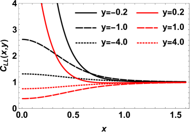
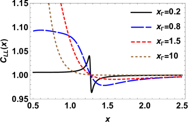
Figure 7: Left panel: CF in LL approximation given in Eq. (29) as a function of $x=kR$, taking different values of $y=R/a$. Right panel: CF in LL approximation given in Eq. (31) as a function of $x=kR$, taking different values of $x_{\Gamma}=\sqrt{\mu\Gamma R^{2}}$. We have considered here the reduced mass $\mu$ of the $D^{*}\pi$ system, and the value of $x_{R}=k_{R}R\simeq 1.3$, which is associated to a resonance localized at $k_{R}\simeq 250$ MeV and $R=1$ fm. The value of $x_{\Gamma}\simeq 0.8$ corresponds to a resonance with $\Gamma\simeq 200$ MeV.

Pursuing further the analysis, to understand the effect of the presence of a resonance at a given momentum $k_{R}$ in the CF, it is more convenient to use Eq. (28) and write Eq. (27) in the form

$$C_{LL}(x) = 1+\frac{\sin^{2}{\delta(k)}}{2x^{2}}\left(e^{-4x^{2}}+\frac{4xF_{2}(2x)}{\sqrt{\pi}}\cot{\delta(k)}\right),$$ (31)

Then, considering that a resonance present at $k_{R}$ generates $\delta(k_{R})=\pi/2$, which when used in Eq. (31) yields $C_{LL}(x_{R})=1+\frac{e^{-4x_{R}^{2}}}{2x_{R}^{2}};\ x_{R}=k_{R}R$. Accordingly, the CF ends up having the following properties (i) $C_{LL}^{\prime}(x_{R})<0$; (ii) $C_{LL}<1$ for $x\gtrsim x_{R}$; and (iii) $C_{LL}\simeq 1$ for large $x_{R}$. To be more didactic, from the analytical expression for the Breit-Wigner-like phase shift, $\delta(E)=\Gamma(E)/(2E_{R}-2E)$ ($\Gamma$ being the width and $E_{R}$ the energy at $k_{R}$), one gets $\cot{\delta(k)}\sim-(x^{2}-x_{R}^{2})/x_{\Gamma}^{2}$, with $x_{\Gamma}^{2}=\mu\Gamma R^{2}$ ($\mu$ being the reduced mass of the two particles in the channel). Thus, the use of this last expression of $\cot{\delta(k)}$ in Eq. (31) can engender in $C_{LL}$ (i) a maximum at $k\lesssim k_{R}$ and a pronounced minimum at $k\gtrsim k_{R}$ for small $x_{\Gamma}$, (ii) a weakened minimum at $k\gtrsim k_{R}$ for intermediate values of $x_{\Gamma}$, and (iii) an almost plateau-like appearance at $k\lesssim k_{R}$ for large $x_{\Gamma}$. This behavior is summarized in Fig. 7 (right panel), in accordance with that in Ref. Albaladejo et al. (2023).

In the end, the form and what can be interpreted from the CF are strongly dependent on the parameters, namely $k_{R},\Gamma,R$, and $a$. We also remark that the application of the LL approximation in the interpretation of the present context must be seen with caution since we treat a coupled-channel problem, which is naturally more complex to analyze and understand. In this sense, it will be helpful to perform comparisons between the single-channel LL and coupled-channel CFs in order to get insights into the reliability of the LL model in the description of this problem.

III.3 Results

III.3.1 CFs in isospin basis

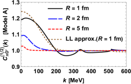
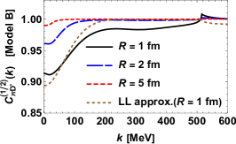
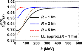
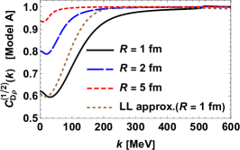
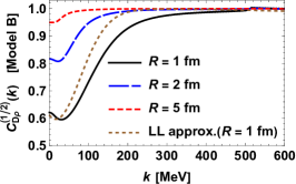
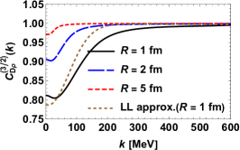
Figure 8: CFs for the $D^{*}\pi$ (top panels) and $D\rho$ (bottom panels) channels as functions of their relative momentum $k$, taking different values of the source size. The left, center, and right panels show the results obtained respectively with $I=1/2$ considering the model A, with $I=1/2$ considering model B, and with $I=3/2$. Recall that the interaction in the isospin 3/2 configuration is repulsive and weaker as compared to the case of isospin 1/2. Thus, no states are formed in the isospin 3/2 case and the amplitudes are obtained from the same model [using Eq. (2)].

In Fig. 8 we plot the results of the correlation functions for the most relevant channels $D^{*}\pi$ and $D\rho$ as functions of their CM momentum $k$, for different values of the range parameter $R$ of the source, considering the following scenarios: $I=1/2$ with the model A, $I=1/2$ with the model B and $I=3/2$. For the sake of comparison and to reach a more profound comprehension concerning our findings, the results with the single-channel LL approximation are also included.

First, one can notice the distinct behavior of the $C_{D^{*}\pi}^{(1/2)}(k)$ when models A or B are employed ( see left and center panels in the upper row of Fig. 8). To start with the discussions, let us focus on the curves related to the smallest source size parameter, $R=1\ \mathrm{fm}$. In the case of model A, at threshold, we have $C_{D^{*}\pi}^{(1/2)}(k=0)>1$, because of the attractive character of this channel and the negative scattering length. In the sequence, as $k$ increases a moderate minimum and a bump are found in the region $220\lesssim k\lesssim 360\ \mathrm{MeV}$. Interestingly, these effects reflect essentially the behavior of the $T_{D^{*}\pi,D^{*}\pi}^{(1/2)}$ amplitude, since the other contributions $T_{D^{*}\pi,D\rho}^{(1/2)}$ and $T_{D^{*}\pi,\bar{K}D_{s}^{*}}$ are negligible, as shown in Fig. 9 . In this sense, the minimum (bump) at $k\gtrsim 250\ \mathrm{MeV}$ ($k\simeq 340\ \mathrm{MeV}$) is associated to the broad peak (dip) in $T_{D^{*}\pi,D^{*}\pi}^{(1/2)}$ at $\sqrt{s}\sim 2304\ \mathrm{MeV}$ ($\sqrt{s}\sim 2405\ \mathrm{MeV}$). Thus, according to our model, the CF encodes the manifestation of the interference between the poles present in $T_{D^{*}\pi,D^{*}\pi}^{(1/2)}$ (see discussions in section II.3.1). However, these effects are no longer prominent for larger values of the source size parameter. Also, a cusp at $k\simeq 518\ \mathrm{MeV}$ is seen and comes from the effect of the $\bar{K}D_{s}^{*}$ threshold. Notably, when compared to the single-channel LL results, these CFs have a similar qualitative behavior only near the threshold, having values larger than one. The $C_{LL}$ does not acquire a minimum from the peak in $T_{D^{*}\pi,D^{*}\pi}^{(1/2)}$, possibly because of its large width (as argued in Sec. III.2).

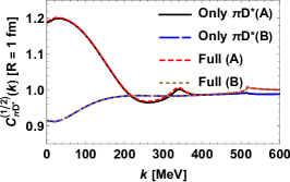
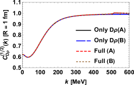
Figure 9: CFs with $I=1/2$ for the $D^{*}\pi$ (left panel) and $D\rho$ (right panel) as functions of their relative momentum $k$ considering the single contribution of the elastic channel (i.e. only $i=j$ of the sum in Eq. (23)), and the total CF.

On the other hand, at the threshold model B generates $C_{D^{*}\pi}^{(1/2)}(k=0)\lesssim 1$, which is compatible with the result expected within the LL approximation when $a_{D^{*}\pi}^{(1/2)}=0.1\ \mathrm{fm}<2.3R$. After that, the CF slightly increases with $k$, and presents almost a plateau shape, which comes from the interference between the states discussed in Sec. II.3.2; then it shows also a cusp at $k\simeq 518\ \mathrm{MeV}$ and goes to one. As in the former model, in this case too the full CF expresses the behavior of the $T_{D^{*}\pi,D^{*}\pi}^{(1/2)}$ amplitude (see the left panel of Fig. 9); and is qualitatively similar to the single-channel LL results only near the threshold, since the $C_{LL}$ goes faster towards unity.

For the $I=3/2$ channel (top, right panel of Fig. 8), at threshold $C_{D^{*}\pi}^{(3/2)}(k)$ starts moderately lower than one. This, considering the value of the scattering length $a_{D^{*}\pi}^{(3/2)}=0.1$ fm, is compatible with the behavior expected within the LL approximation when $a_{D^{*}\pi}^{(3/2)}=0.1\ \mathrm{fm}<2.3R$. After that, the CF increases with the augmentation of $k$ and goes to one; no other effect appears as no state is present.

Now we move on to the channel $D\rho$ (bottom panels of Fig. 8), whose scattering length has an imaginary component. We do not see sizable differences in the $C_{D\rho}^{(1/2)}(k)$ obtained considering the models A and B (as expected from the similarity of the $D\rho$ amplitude in the two models). Noticing that $Re[a_{D\rho}^{(1/2)}]=0.44\ \mathrm{fm}<2.3R$, then one can expect that $C_{D^{*}\pi}^{(1/2)}(k=0)<1$. However, when compared with the results for $D^{*}\pi$ in model B, the CF experiences a substantial dip. Taking advantage of the analysis in the previous section, this may be interpreted as the influence of the narrow state present in the $T_{D\rho,D\rho}^{(1/2)}$ amplitude below the $D\rho$ threshold, which as shown in Fig. 9, provides the relevant contribution. When compared to the single-channel LL approximation, at threshold $C_{D\rho}^{(1/2)}(k)$ is quite near $C_{LL}$ but goes more slowly towards unity.

III.3.2 CFs in physical basis

We remark that the CFs presented so far, for the relevant channels $D^{*}\pi$ and $D\rho$, are in the isospin basis. Therefore, in order to provide measurable CFs, we need to express them on the particle basis. In the case of $D^{*}\pi$ (the case of $D\rho$ is completely analogous), we consider the isospin-doublet of the vector charmed meson and isospin-triplet of the pion as $D\equiv(|D^{*+}\rangle,-|D^{*0}\rangle)$ and $\pi\equiv(-|\pi^{+}\rangle,|\pi^{0}\rangle,|\pi^{-}\rangle)$, respectively. Then, for $D^{*}\pi$-states with $I_{3}=+1/2$, the particle basis is given by ${|D^{*0}\pi^{+}\rangle,|D^{*+}\pi^{0}\rangle}$, which is related to the isospin basis through (denoting states as $|D\pi,I\rangle$)

$$|D^{*0}\pi^{+}\rangle = -\left[\sqrt{\frac{2}{3}}\left|D\pi,\frac{1}{2}\right\rangle-\sqrt{\frac{1}{3}}\left|D\pi,\frac{3}{2}\right\rangle\right],$$

$$|D^{*+}\pi^{0}\rangle = \sqrt{\frac{1}{3}}\left|D\pi,\frac{1}{2}\right\rangle+\sqrt{\frac{2}{3}}\left|D\pi,\frac{3}{2}\right\rangle.$$ (32)

With these last expressions, we can write the two-particle wave function for charged states as

$$\Psi_{D^{*0}\pi^{+}\to D^{*0}\pi^{+}} \equiv \frac{2}{3}\Psi_{D^{*}\pi}^{\left(\frac{1}{2}\right)}+\frac{1}{3}\Psi_{D^{*}\pi}^{\left(\frac{3}{2}\right)},$$

$$\Psi_{D^{*+}\pi^{0}\to D^{*0}\pi^{+}} \equiv -\frac{\sqrt{2}}{3}\Psi_{D^{*}\pi}^{\left(\frac{1}{2}\right)}+\frac{\sqrt{2}}{3}\Psi_{D^{*}\pi}^{\left(\frac{3}{2}\right)},$$

$$\Psi_{D^{*0}\pi^{+}\to D^{*+}\pi^{0}} \equiv -\frac{\sqrt{2}}{3}\Psi_{D^{*}\pi}^{\left(\frac{1}{2}\right)}+\frac{\sqrt{2}}{3}\Psi_{D^{*}\pi}^{\left(\frac{3}{2}\right)},$$

$$\Psi_{D^{*+}\pi^{0}\to D^{*+}\pi^{0}} \equiv \frac{1}{3}\Psi_{D^{*}\pi}^{\left(\frac{1}{2}\right)}+\frac{2}{3}\Psi_{D^{*}\pi}^{\left(\frac{3}{2}\right)},$$ (33)

where the superscript on $\Psi$ indicates the related isospin. As a consequence, using Eq. (33) in  (23) we get

$$C_{D^{*0}\pi^{+}} \equiv C_{D^{*0}\pi^{+}\to D^{*0}\pi^{+}}+C_{D^{*+}\pi^{0}\to D^{*0}\pi^{+}}=\frac{2}{3}C_{D^{*}\pi}^{\left(\frac{1}{2}\right)}+\frac{1}{3}C_{D^{*}\pi}^{\left(\frac{3}{2}\right)},$$

$$C_{D^{*+}\pi^{0}} \equiv C_{D^{*0}\pi^{+}\to D^{*+}\pi^{0}}+C_{D^{*+}\pi^{0}\to D^{*+}\pi^{0}}=\frac{1}{3}C_{D^{*}\pi}^{\left(\frac{1}{2}\right)}+\frac{2}{3}C_{D^{*}\pi}^{\left(\frac{3}{2}\right)}.$$ (34)

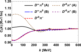
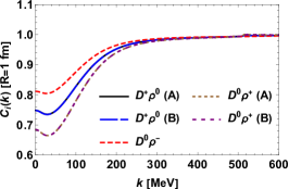
Figure 10: CFs for the physical $D^{*}\pi$ and $D\rho$ states defined in Eq. (32) in both cases of models A and B, taking the source size parameter $R=1$ fm. The CFs $C_{D^{*0}\pi^{-}}(k)$ and $C_{D^{0}\rho^{-}}(k)$, equivalent to the corresponding $C_{i}^{(3/2)}(k)$, are also plotted.

We show the CFs for the $D^{*}\pi$ and $D\rho$ states in the particle basis defined in Eq. (34), in Fig. 10, for both models A and B. The CFs $C_{D^{*0}\pi^{-}}(k)$ and $C_{D^{0}\rho^{-}}(k)$ are also plotted; since these states have $I_{3}=-3/2$, their corresponding CFs are naturally equal to $C_{i}^{(3/2)}(k)$. It can be seen that for model A the features of the $T_{D^{*}\pi,D^{*}\pi}^{(1/2)}$ amplitude are more notable in the channel $D^{*0}\pi^{+}$, because of the bigger weight of the $I=1/2$ channel in its wave function. In contrast, for model B there is no sizable difference among the channels $D^{*0}\pi^{+},D^{*+}\pi^{0}$ and $D^{*0}\pi^{-}$, due to the similarity among $C_{D^{*}\pi}^{(1/2)}(k)$ and $C_{D^{*}\pi}^{(3/2)}(k)$. Going to the scenario of $D\rho$, the difference coming from the isospin weights produces $C_{D^{+}\rho^{0}}(k)$ closer to one at threshold than $C_{D^{0}\rho^{+}}(k)$. Hence, one can conclude that the $D^{*0}\pi^{+}$ and $D^{0}\rho^{+}$ channels are more appropriate to test both models.

In the end, we stress the main conclusion of this study, namely: our findings suggest that $C_{D^{*}\pi}(k)$ and $C_{D\rho}(k)$ might encode sufficiently identifiable signatures of the $D_{1}(2430)^{0}$ and $D_{1}(2420)$ states when smaller sources are considered. It should be emphasized that if the femtoscopic analysis for the mentioned channels is done and the measured genuine CFs have similar behavior to those obtained here, then it is possible to say that this work provides a framework compatible with the existence of both broad and narrow states. In this sense, it would be interesting to confront these CFs with data collected in future high precision experiments.

IV Conclusions

The main conclusions of the discussions presented in this work can be summarized as follows.

• The information on the properties of the two lightest $D_{1}$ states comes mostly from fits made to the experimental data on the $D^{*}\pi$ invariant mass, which gets contribution from several charm states. Such a procedure attributes similar masses but very different widths to the two of them, which indicates that the two states must have something different in their nature.

• There exists information on the scattering length, determined in the lattice QCD calculations, for the $D^{*}\pi$ and $D\pi$ channels. Both values are very similar. Several model calculations constrain their parameters using the former information and determine the $D\pi$ scattering length in the infinite volume by using physical masses. It can be argued that the scattering lengths for $D\pi$ and $D^{*}\pi$ can be similar, which provides another valuable information on the study of the $D^{*}\pi$ system.

• A value for the $D\pi$ scattering length is also available from heavy ion collisions but it does not agree with those mentioned in the previous point.

• With the purpose of understanding the properties of the two enigmatic $D_{1}$ states, we consider a model where different meson-meson interactions and a bare quark model pole constitute the lowest order amplitudes. Such amplitudes are used as kernels to solve the Bethe-Salpeter equation in a coupled channel approach. Consequently, a narrow pole is found to get generated by the hadron dynamics and is related to $D_{1}(2420)$. A broader pole is also found, whose properties match those of $D_{1}(2430)$ when both hadron dynamics and a bare quark-model pole are considered.

• To contemplate the two aforementioned disagreeing values of the scattering lengths, we present two models. The two differ in the parameters related to the bare quark-model pole.

• Using such amplitudes we determine correlation functions and find that such information on the $D^{*0}\pi^{+}$ and $D^{*0}\rho^{+}$ channels, determined from smaller source sizes, can bring useful information on the subject.

V acknowledgements

This work is partly supported by the Brazilian agencies CNPq (L.M.A.: Grant Numbers 309950/2020-1, 400215/2022-5, 200567/2022-5), FAPESP (K.P.K.: Grant Number 2022/08347-9; A. M. T.: Grant number 2023/01182-7); FAPESB (L.M.A.: Grant Number INT0007/2016); and CNPq/FAPERJ under the Project INCT-Física Nuclear e Aplicações (Contract No. 464898/2014-5).

References

- Acharya et al. (2023a) S. Acharya et al. (ALICE), Phys. Lett. B 844, 137223 (2023a), arXiv:2204.10258 [nucl-ex] .
- Acharya et al. (2023b) S. Acharya et al. (ALICE), Phys. Rev. C 107, 054904 (2023b), arXiv:2211.15194 [nucl-ex] .
- Acharya et al. (2023c) S. Acharya et al. (ALICE), Phys. Lett. B 845, 138145 (2023c), arXiv:2305.19093 [nucl-ex] .
- Fabbietti et al. (2021) L. Fabbietti, V. Mantovani Sarti, and O. Vazquez Doce, Ann. Rev. Nucl. Part. Sci. 71, 377 (2021), arXiv:2012.09806 [nucl-ex] .
- Lisa et al. (2005) M. A. Lisa, S. Pratt, R. Soltz, and U. Wiedemann, Ann. Rev. Nucl. Part. Sci. 55, 357 (2005), arXiv:nucl-ex/0505014 .
- Workman et al. (2022) R. L. Workman et al. (Particle Data Group), PTEP 2022, 083C01 (2022).
- Aaij et al. (2015) R. Aaij et al. (LHCb), Phys. Rev. D 92, 012012 (2015), arXiv:1505.01505 [hep-ex] .
- Abe et al. (2004) K. Abe et al. (Belle), Phys. Rev. D 69, 112002 (2004), arXiv:hep-ex/0307021 .
- Godfrey and Isgur (1985) S. Godfrey and N. Isgur, Phys. Rev. D 32, 189 (1985).
- Ferretti and Santopinto (2018) J. Ferretti and E. Santopinto, Phys. Rev. D 97, 114020 (2018), arXiv:1506.04415 [hep-ph] .
- Du et al. (2018) M.-L. Du, M. Albaladejo, P. Fernández-Soler, F.-K. Guo, C. Hanhart, U.-G. Meißner, J. Nieves, and D.-L. Yao, Phys. Rev. D 98, 094018 (2018), arXiv:1712.07957 [hep-ph] .
- Abreu et al. (2019) L. M. Abreu, A. G. Favero, F. J. Llanes-Estrada, and A. G. Sánchez, Phys. Rev. D 100, 116012 (2019), arXiv:1908.11154 [hep-ph] .
- Lang and Wilson (2022) N. Lang and D. J. Wilson (Hadron Spectrum), Phys. Rev. Lett. 129, 252001 (2022), arXiv:2205.05026 [hep-ph] .
- Di Pierro and Eichten (2001) M. Di Pierro and E. Eichten, Phys. Rev. D 64, 114004 (2001), arXiv:hep-ph/0104208 .
- Bardeen et al. (2003) W. A. Bardeen, E. J. Eichten, and C. T. Hill, Phys. Rev. D 68, 054024 (2003), arXiv:hep-ph/0305049 .
- Colangelo et al. (2004) P. Colangelo, F. De Fazio, and R. Ferrandes, Mod. Phys. Lett. A 19, 2083 (2004), arXiv:hep-ph/0407137 .
- Mehen and Springer (2005) T. Mehen and R. P. Springer, Phys. Rev. D 72, 034006 (2005), arXiv:hep-ph/0503134 .
- Ni et al. (2022) R.-H. Ni, Q. Li, and X.-H. Zhong, Phys. Rev. D 105, 056006 (2022), arXiv:2110.05024 [hep-ph] .
- Kolomeitsev and Lutz (2004) E. E. Kolomeitsev and M. F. M. Lutz, Phys. Lett. B 582, 39 (2004), arXiv:hep-ph/0307133 .
- Guo et al. (2007) F.-K. Guo, P.-N. Shen, and H.-C. Chiang, Phys. Lett. B 647, 133 (2007), arXiv:hep-ph/0610008 .
- Gamermann and Oset (2007) D. Gamermann and E. Oset, Eur. Phys. J. A 33, 119 (2007), arXiv:0704.2314 [hep-ph] .
- Malabarba et al. (2023) B. B. Malabarba, K. P. Khemchandani, A. Martinez Torres, and E. Oset, Phys. Rev. D 107, 036016 (2023), arXiv:2211.16222 [hep-ph] .
- Coito et al. (2011) S. Coito, G. Rupp, and E. van Beveren, Phys. Rev. D 84, 094020 (2011), arXiv:1106.2760 [hep-ph] .
- Burns (2014) T. J. Burns, Phys. Rev. D 90, 034009 (2014), arXiv:1403.7538 [hep-ph] .
- Note (1) The position of the corresponding pole in Ref. Gamermann and Oset (2007) was MeV, which is in better agreement with the properties of . However, recall that the narrow pole found in Ref. Gamermann and Oset (2007) appears at 2526 MeV which is far from the mass of .
- Mohler et al. (2013) D. Mohler, S. Prelovsek, and R. M. Woloshyn, Phys. Rev. D 87, 034501 (2013), arXiv:1208.4059 [hep-lat] .
- Liu et al. (2013) L. Liu, K. Orginos, F.-K. Guo, C. Hanhart, and U.-G. Meissner, Phys. Rev. D 87, 014508 (2013), arXiv:1208.4535 [hep-lat] .
- Guo et al. (2019) Z.-H. Guo, L. Liu, U.-G. Meißner, J. A. Oller, and A. Rusetsky, Eur. Phys. J. C 79, 13 (2019), arXiv:1811.05585 [hep-ph] .
- Guo et al. (2009) F.-K. Guo, C. Hanhart, and U.-G. Meissner, Eur. Phys. J. A 40, 171 (2009), arXiv:0901.1597 [hep-ph] .
- Abreu et al. (2011) L. M. Abreu, D. Cabrera, F. J. Llanes-Estrada, and J. M. Torres-Rincon, Annals Phys. 326, 2737 (2011), arXiv:1104.3815 [hep-ph] .
- Geng et al. (2010) L. S. Geng, N. Kaiser, J. Martin-Camalich, and W. Weise, Phys. Rev. D 82, 054022 (2010), arXiv:1008.0383 [hep-ph] .
- (32) (Alice), https://indico.cern.ch/event/883427/contributions/4921802/attachments/2480998/4259088/HFwincLaura.pdf.
- (33) F. Grosa (ALICE), “ALICE determines the scattering parameters of D mesons with light-flavor hadrons,” https://indico.cern.ch/event/895086/contributions/4715876/.
- (34) D. Battistini (ALICE), “Measurement of scattering parameters governing the residual strong interaction between charm and light hadrons,” https://indico.cern.ch/event/1198609/contributions/5363368/attachments/2651649/4596659/2023.
- (35) L. Fabbietti, F. Grosa, E. Chizzali, and D. Battistini, “Measurement of scattering parameters governing the residual strong interaction between charm and light hadrons,” https://indico.cern.ch/event/883427/contributions/4921802/attachments/2480998/4259088/HFwincLaura.pdf.
- Bando et al. (1985) M. Bando, T. Kugo, S. Uehara, K. Yamawaki, and T. Yanagida, Phys. Rev. Lett. 54, 1215 (1985).
- Bando et al. (1988) M. Bando, T. Kugo, and K. Yamawaki, Phys. Rept. 164, 217 (1988).
- Meissner (1988) U. G. Meissner, Phys. Rept. 161, 213 (1988).
- Harada and Yamawaki (2003) M. Harada and K. Yamawaki, Phys. Rept. 381, 1 (2003), arXiv:hep-ph/0302103 .
- Note (2) The pole appears on the second Riemann sheet of the , though it lies below the corresponding threshold.
- Aubert et al. (2006) B. Aubert et al. (BaBar), Phys. Rev. D 74, 012001 (2006), arXiv:hep-ex/0604009 .
- Koonin (1977) S. E. Koonin, Phys. Lett. B 70, 43 (1977).
- Pratt (1986) S. Pratt, Phys. Rev. D 33, 1314 (1986).
- Lednicky and Lyuboshits (1981) R. Lednicky and V. L. Lyuboshits, Yad. Fiz. 35, 1316 (1981).
- Lednicky et al. (1998) R. Lednicky, V. V. Lyuboshits, and V. L. Lyuboshits, Phys. At. Nucl. 61, 2950 (1998).
- Note (3) Eq. (23) is also called by some authors like those from Refs. Kamiya et al. (2022) as Koonin\IeC–Pratt\IeC–Lednicky\IeC–Lyuboshits\IeC–Lyuboshits formula due to subsequent contributions Lednicky and Lyuboshits (1981); Lednicky et al. (1998).
- Vidana et al. (2023) I. Vidana, A. Feijoo, M. Albaladejo, J. Nieves, and E. Oset, Phys. Lett. B 846, 138201 (2023), arXiv:2303.06079 [hep-ph] .
- Feijoo et al. (2023) A. Feijoo, L. R. Dai, L. M. Abreu, and E. Oset, (2023), arXiv:2309.00444 [hep-ph] .
- Albaladejo et al. (2023) M. Albaladejo, J. Nieves, and E. Ruiz-Arriola, Phys. Rev. D 108, 014020 (2023), arXiv:2304.03107 [hep-ph] .
- Kamiya et al. (2022) Y. Kamiya, K. Sasaki, T. Fukui, T. Hyodo, K. Morita, K. Ogata, A. Ohnishi, and T. Hatsuda, Phys. Rev. C 105, 014915 (2022), arXiv:2108.09644 [hep-ph] .
- Note (4) Once again, we emphasize that our sign convention is different from that of Ref. Albaladejo et al. (2023), i.e. , which gives a different sign in the last term between parentheses.
- Note (5) This finding is in agreement with the result on the amplitude discussed in section II.3.1 and II.3.2. An equivalent effect is also found in the femtoscopic analysis of the coupled-channel and interactions Kamiya et al. (2022).