Fast, Scalable, Warm-Start Semidefinite Programming
with Spectral Bundling and Sketching
Abstract
While semidefinite programming (SDP) has traditionally been limited to moderate-sized problems, recent algorithms augmented with matrix sketching techniques have enabled solving larger SDPs. However, these methods achieve scalability at the cost of an increase in the number of necessary iterations, resulting in slower convergence as the problem size grows. Furthermore, they require iteration-dependent parameter schedules that prohibit effective utilization of warm-start initializations important in practical applications with incrementally-arriving data or mixed-integer programming. We present Unified Spectral Bundling with Sketching (USBS), a provably correct, fast and scalable algorithm for solving massive SDPs that can leverage a warm-start initialization to further accelerate convergence. Our proposed algorithm is a spectral bundle method for solving general SDPs containing both equality and inequality constraints. Moveover, when augmented with an optional matrix sketching technique, our algorithm achieves the dramatically improved scalability of previous work while sustaining convergence speed. We empirically demonstrate the effectiveness of our method across multiple applications, with and without warm-starting. For example, USBS provides a 500x speed-up over the state-of-the-art scalable SDP solver on an instance with over 2 billion decision variables.
1 Introduction
Semidefinite programming (SDP) is a convex optimization paradigm capable of modeling or approximating many practical problems in combinatorial optimization [3], neural network verification [71, 26], robotics [73], optimal experiment design [92], VLSI [91], and systems and control theory [15]. Despite their widespread applicability, practitioners often dismiss the use of SDPs under the presumption that optimization is intractable at real-world scale. This assumption is grounded in the prohibitively high computational complexity of standard SDP solvers [5, 90].
The main challenge when solving SDPs with standard constrained optimization approaches is the high cost of projection onto the feasible region. Projecting a symmetric matrix onto the semidefinite cone requires a full eigendecomposition, an operation that scales cubicly with the problem dimension. The high computational cost of this single operation severely limits the applicability of projected gradient and ADMM-based approaches [18, 69]. Interior point methods, the de facto approach for solving small-to-moderate sized SDPs, require even more computational resources.
Projection-free and conditional gradient-based methods have been proposed to avoid the computational burden of projecting iterates onto the semidefinite cone [106, 104, 10]. These methods avoid projection onto the feasible region with various techniques including subgradient descent in the dual space and a conditional gradient method on an unconstrained augmented objective function. The bulk of the computational burden for these methods is typically an extreme eigenvector calculation. The scalablity of these methods is still limited, despite the improved per-iteration complexity, since they require storing the entire primal matrix which scales quadratically with the problem dimension.
The most well-known method for scaling semidefinte programming without storing the entire primal matrix in memory is the Burer–Monteiro (BM) factorization heuristic [21]. The core idea of the BM method is to explicitly control the memory usage by restricting the primal matrix to a low-rank factorization. However, this method sacrifices the convexity of the problem for scalability. In some cases, the BM method either requires having a high rank factorization, leading to burdensome memory requirements, or risks optimization getting stuck in local minima [97]. Yurtsever et al. [107] extend the conditional gradient augmented Lagrangian approach [106] with a matrix sketching technique. This approach avoids storing the entire primal matrix while maintaining the convexity of the problem leading to provable convergence for general SDPs. In addition, this method uses iteration-dependent parameters prohibiting it from reliably leveraging a warm-start initialization.
Spectral bundle methods, first proposed by Helmberg and Rendl [42], are an appealing framework for solving SDPs due to their low per-iteration computational complexity and fast empirical convergence. While several spectral bundle methods have been presented in the literature [41, 8, 43, 28], previous work considers SDPs with either only equality constraints or only inequality constraints. Furthermore, the lack of an efficient standalone implementation has prevented the evaluation of spectral bundle method on massive SDPs.
Contributions.
We present USBS, a unified spectral bundle method designed for a broader class of SDPs and show it is a practical approach for solving large problem instances quickly. USBS flexibly allows the user to control the trade-off between per-iteration complexity and the empirical speed at which the algorithm converges. In addition, USBS can be augmented with a matrix sketching technique that can dramatically improve the scalability of the algorithm while maintaining its fast convergence. We demonstrate the empirical efficacy of our proposed spectral bundle method on three types of practical large SDPs seeing extraordinary performance improvements in comparison with the previous state-of-the-art scalable solver for general SDPs. For example, USBS is able to obtain a quality solution to an SDP with over decision variables while the previous state-of-the-art fails to reach an accurate solution within 72 hours. In addition, we see a 500x speedup over the previous state-of-the-art on an instance with 2 billion decision variables. Finally, we find that warm-starting can lead to more than a 100x speedup in the convergence of USBS as compared to cold-starting while the previous state-of-the-art often is not able to reliably take advantage of a warm-start initialization. We provide a standalone implementation of the algorithm in pure JAX [19, 36], enabling efficient execution on various hardware (CPU, GPU, TPU) and wide-spread use.
2 Preliminaries
2.1 Semidefinite Programming
We begin with the notation necessary to define the semidefinite programming problem. Let be the set of all real symmetric matrices and be the positive semidefinite cone. Let denote the standard inner product for vectors and the Frobenius inner product for matrices. For any matrix , let denote the maximum eigenvalue of and let denote the trace of . Let be a given linear operator and be its adjoint, i.e. for any and , which take the following form,
for given matrices . For any given , let denote the linear operator restricted to matrices for and to be the corresponding subset of rows for any . In general, we utilize to extract the corresponding indices from any vector in . Finally, let be the compliment of .
Given fixed , , , and , the primal (P) and dual (D) semidefinite programs can be written as follows:
| (P) |
| (D) |
Note that while all SDPs of this form can technically be written as equality constrained SDPs (i.e. standard-form SDPs), doing so in practice is ill-advised since the problem dimension, , grows by one for every inequality constraint. In addition, we also represent the primal feasibility set as the convex set , and measure the primal infeasibility . We use to denote the Euclidean distance from a point to a closed set and to denote the Euclidean projection of onto . Equivalently,
We denote the solution sets of (P) and (D) by and , respectively. We make the standard assumption that (P) and (D) satisfy strong duality, namely that the solution sets and are nonempty, compact, and every pair of solutions has zero duality gap: . Strong duality holds whenever Slater’s condition holds and is a surjective linear operator. Additionally, we say that the SDP satisfies strict complementarity if there exists such that for induced dual slack matrix , Strict complementarity is satisfied by generic SDPs [4] and many well-structured SDPs [29]. Lastly, we denote the maximum nuclear norm of the primal solution set as .
In many important applications, SDPs take a highly structured and sparse forms that admit low-rank solutions. The cost matrix is often sparse, containing many fewer than non-zero entries. Additionally, the number of primal constraints is often much less , being proportional to or the number of non-zero entries in . We would like to exploit these features with a provably correct, fast and scalable optimization algorithm that can solve any SDP.
2.2 Proximal Bundle Method
Proximal bundle methods [55, 63, 33, 49] are a class of optimization algorithms for solving unconstrained convex minimization problems of the form , where is a proper closed convex function that attains its minimum value, , on some nonempty set. At each iteration, the proximal bundle method proposes an update to the current iterate by applying a proximal step to an approximation of the objective function, :
| (1) |
where . The next iterate is set equal to only when the decrease in the objective value is at least a fixed fraction of the decrease predicted by the model , i.e.
| (2) |
for some fixed . The iterations where (2) is satisfied (and thus, ) are referred to as descent steps. Otherwise, the algorithm takes a null step and sets . Regardless of whether (2) is satisfied or not, is used to construct the next model .
Model Requirements.
The model can take many forms, but is usually constructed using subgradients of at past and current iterates. Let denote the subdifferential of at (i.e. the set of subgradients of evaluated at a point ). Following prior work, we require the next model to satisfy the following mild assumptions:
-
1.
Minorant.
(3) -
2.
Subgradient lower bound. For any ,
(4) -
3.
Model subgradient lower bound. The first order optimality conditions for (1) gives the subgradient . After a null step ,
(5)
The first two conditions serve to guarantee that a new model integrates first-order information from the objective at . The third condition demands the new model to preserve approximation accuracy exhibited by the preceding model.
3 Unified Spectral Bundling
In this section, we will present USBS, our proposed algorithm for solving the SDP defined in (P) and (D), Our proposed spectral bundle method is a unified algorithm for solving SDPs with both equality and inequality constraints and can be integrated with a matrix sketching technique for dramatically improved scalability as demonstrated in Section 4. To apply the proximal bundle method, we consider consider minimizing the following unconstrained objective
| (pen-D) |
where and . Minimizing (pen-D) is equivalent to optimizing (D) in the sense that the optimal solution set and objective are the same (Appendix A.1). In the following subsections, we will detail how the model is constructed and how to compute the candidate iterates.
3.1 Spectral Bundle Model
The form of (pen-D) is not quite conducive to defining the model and solving for the candidate iterate . To address this, we will consider an equivalent formulation to (pen-D) that is more amenable to this effort. For any fixed , let be the trace constrained subset of the primal domain. Let be the domain of the dual slack variable for the indicator function . Then, we can rewrite the following equivalent formulation to (pen-D)
| (6) |
We derive this equivalent formulation in Appendix A.2.
Defining the model.
This equivalent formulation is clearly just as difficult to optimize as (pen-D), but is helpful in defining the model we will utilize in the spectral bundle method. The main idea is to consider (6) over a low-dimensional subspace of such that (3), (4), and (5) are satisfied. The subspace we will consider at step is parameterized by matrices and and is defined as follows
| (7) |
The matrix has orthonormal column vectors, where is a small user defined parameter. The columns of are partitioned into current eigenvectors and orthonormal vectors representing past spectral information. Regardless of the setting of and , the columns of will always include a maximum eigenvector of , which also means . For scalability reasons, we expect to be relatively small. The matrix is a carefully selected weighted sum of past spectral bounds such that and enables the last model condition (5) to be satisfied. Hence, the model is
| (8) |
We show that this model satisfies the conditions (3), (4), and (5) in Appendix D.1.
Updating the model.
Independent of whether a descent step or null step is taken, the model needs to be updated. At every step, we solve the following minimax problem
| (9) |
where is the minimax solution. The structure of allows us to rewrite as
| (10) |
To compute and we first compute an eigendecomposition of to separate current and past spectral information as follows
| (11) |
where is a diagonal matrix containing the largest eigenvalues and contains the corresponding eigenvectors. The diagonal matrix contains the remaining eigenvalues and the corresponding eigenvectors are contained in the columns of . Given this decomposition, we set the next model’s as follows
| (12) |
In the case that , observe that for all . To update , we first compute the top orthonormal eigenvectors of . Then, we set to orthonormal vectors that span the columns of as follows
| (13) |
where we can use QR decomposition to orthonormalize the vectors. If , orthonormalization is unnecessary and we just set .
3.2 Computing the Candidate Iterate
We will now discuss how to compute the candidate iterate by applying a proximal step to the current approximation of the objective function (i.e. solve (1)). We show in Appendix A.3 that the candidate iterate can be computed as
| (14) |
where is the solution to the following optimization problem
| (15) |
where we define To solve for , we propose using the alternating maximization algorithm. After initializing , the the following update steps are repeated until convergence:
| (16) | ||||
| (17) |
Clearly is smooth, and in this case the alternating maximization algorithm is known to converge at a rate [14]. If happens to also be strongly concave, the rate improves to [61]. We solve (16) using a primal-dual interior point method derived in Appendix B.2.
Feasibility of .
If we substitute into (14), it can be seen that the candidate is always feasible
and is also complementary to the dual slack variable , i.e. This view allows us to see that we can equivalently express the candidate iterate as
The complete algorithm is detailed in Algorithm 1. Notice that USBS has no iteration-dependent step-sizes or parameters, making it more amenable to effectively utilize a warm-start initialization. It is important to note that the main cost of computing and is a maximum eigenvalue computation of and , respectively. Lastly, we compute using a primal-dual interior point method derived in Appendix B.1.
Convergence Rate.
Under any setting of the parameters, Theorem 3.1 guarantees sublinear convergence for both primal and dual problems, showing that the iterates and converge in terms of objective gap and feasilibity.
Theorem 3.1.
Suppose strong duality holds. For any fixed , and , USBS produces iterates and such that for any ,
| penalized dual optimality: | |||
| primal feasiblity: | |||
| dual feasiblity: | |||
| primal-dual optimality: |
by some iteration . And, if strict complementarity holds, then these conditions are achieved by some iteration . Additionally, if Slater’s condition holds and is unique, then the approximate primal feasibility and approximate primal-dual optimality respectively improve to
The proof is of this theorem is given in Appendix D.
4 Scaling with Matrix Sketching
The memory required to store the primal iterates (similarly ) is prohibitive to scaling SDPs to large problem instances. We will utilize a Nyström sketch [87, 37, 39, 56] to track a compressed low-rank projection of the primal iterate as it evolves which at any iteration can be used to compute a provably accurate low-rank approximation of .
First, notice that the operations carried out by USBS do not require explicitly storing . In fact, if we are not interested in the primal iterates and we only want to solve the dual problem (e.g. in the case where we want to test the feasbility of the primal problem), we only need to store , , and , which can be efficiently maintained with low-rank updates to (see Appendix C for more details). This means if we are interested in the primal iterates, our storage of is independent from the operations of USBS.
Consider any iterate . Let be a parameter that trades off accuracy for scalability. To construct the Nyström sketch, we sample a random projection matrix such that are sampled i.i.d. The projection of , or sketch, can be computed as . We can efficiently maintain this sketch under low-rank updates made to ,
| (18) | ||||
Given the sketch and the projection matrix , we can compute a rank- approximation to . It is important to note that by applying this Nyström sketching technique the only approximation error is in the approximation of , and all of the error is constant (i.e. the error does not compound over time) and comes only from the projection matrix (and the choice of ). See Appendix C for more details.
5 Experiments
We evaluate USBS on three different problem types with and without warm-starting strategies against the scalable semidefinite programming algorithm CGAL [106, 107] (with sketching). Yurtsever et al. [107] perform an extensive evaluation against strong SDP solvers, including SeDuMi [81], SDPT3 [86], Mosek [9], SDPNAL+[103], and the BM factorization heuristic [21]. They show on several applications that CGAL with sketching is by far the standard against which to compare for scalable semidefinite programming.
| fe_sphere | hi2010 | fe_body | me2010 | fe_tooth | 598a | 144 | auto | netherlands_osm | 333SP | |
|---|---|---|---|---|---|---|---|---|---|---|
| 16K | 25K | 45K | 70K | 78K | 111K | 145K | 449K | 2.2M | 3.7M | |
| 115K | 149K | 372K | 405K | 983K | 1.6M | 2.3M | 7.1M | 7.1M | 25.9M |
We consider the primal iterate an -approximate solution if the relative primal objective suboptimality and relative infeasibility is less than , i.e.
| (19) |
Computing the relative infeasibility is simple. We do not usually have access to the optimal primal objective value to compute the relative primal objective suboptimality, but we can compute an upper bound. See (69) for how we compute this upper bound. We include further experimental details in Appendix E and results in Appendix F.
5.1 MaxCut
The MaxCut problem is a fundamental combinatorial optimization problem and its SDP relaxation is a common test bed for SDP solvers. Given an undirected graph, the MaxCut is a partitioning of the vertices into two sets such that the number of edges between the two subsets is maximized. The MaxCut SDP relaxation [38] is as follows
| (20) |
where is the graph Laplacian, extracts the diagonal of a matrix into a vector, and is the all-ones vector. In many instances of MaxCut, the graph Laplacian is sparse and the optimal solution is low-rank. This means that we can represent the MaxCut instance with far less than memory and leverage sketching the primal matrix to improve scalability temendously.
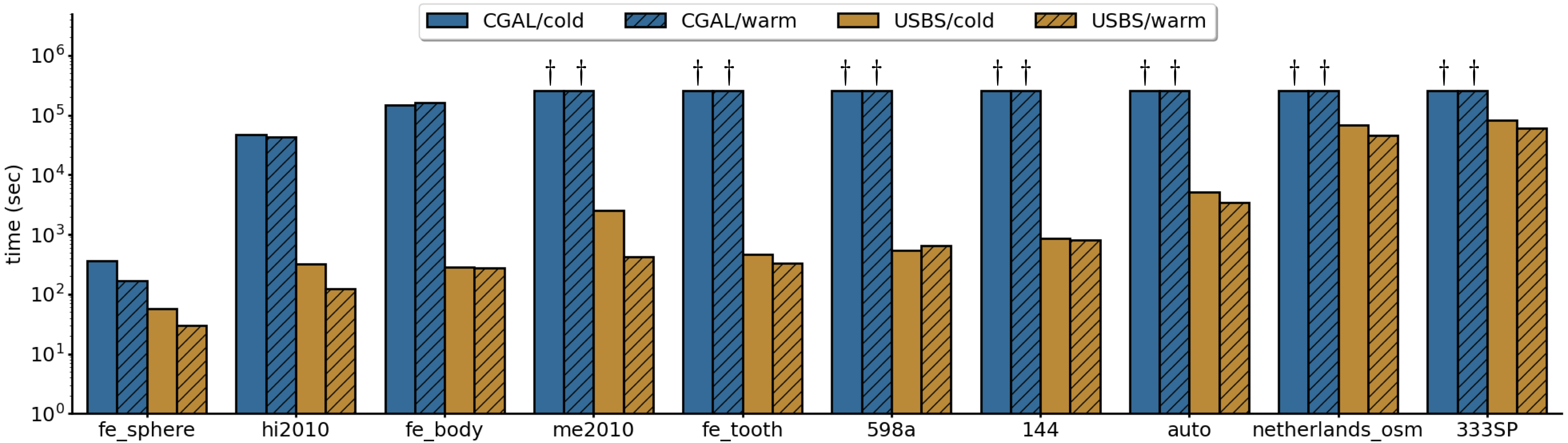
We evaluate the CGAL and USBS with and without warm-starting on ten instances from the DIMACS10 [11] where and the number of edges in each graph are shown in Table 1. We warm-start each method by dropping the last 1% of vertices from the graph, resulting in a graph with 99% of the vertices. We pad the solution from the 99%-sized problem with zeros and rescale as necessary to create the warm-start initialization. Figure 1 displays the time (in seconds) taken by CGAL and USBS, with and without warm-starting on each of the ten instances, where .
5.2 Quadratic Assignment Problem
The quadratic assignment problem (QAP) is a very difficult but fundamental class of combinatorial optimization problems containing the traveling salesman problem, max-clique, bandwidth problems, and facilities location problems among others [59]. SDP relaxations have been shown to facilitate finding good solutions to large QAPs [109]. For any QAP instance, the goal is to optimize an assignment matrix which aligns a weight matrix and distance matrix . The number of assignment matrices is , so a brute-force search becomes quickly intractable as n grows. Generally, QAP instances with are intractable to solve exactly.
There are many SDP relaxtions for QAPs, but we consider the one presented by [107] and inspired by [45, 20] which is
| (21) | ||||
where denotes the Kronecker product, and denote the partial trace over the first and second systems of Kronecker product respectively, extracts the entries of Y corresponding to the nonzero entries of , and stacks the columns of a matrix one on top of the other to form a vector. In many cases, one of or is sparse (i.e. nonzero entries) resulting in total constraints for the SDP.
The primal variable has dimension and as a result the SDP relaxation has decision variables. Given the aggressive growth in complexity, most SDP based algorithms have difficulty operating on instances where . To reduce the number of decision variables, we sketch with , resulting in entries in the sketch and the same number of constraints in most natural instances. We show that this enables CGAL and USBS to scale to instances where (1.5 billion decision variables).
We evaluate CGAL and USBS on select large instances from QAPLIB [23] and TSPLIB [72] ranging in size from 136 to 198. Provided with each of these QAP instances is the known optimum. For many instances, we find that the quality of the permutation matrix produced by the rounding procedure does not entirely correlate with the quality of the iterates with respect to the SDP (21). Thus, we apply the rounding procedure at every iteration of both CGAL and USBS. Our metric for evaluation is relative gap which is computed as follows
We report the lowest value so far of relative gap as best relative gap. CGAL [107] is shown to obtain significantly smaller best relative gap than CSDP [20] and PATH [108] on most instances, and thus, is a strong baseline for achieving high quality approximate solutions.
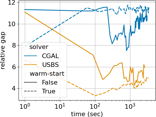
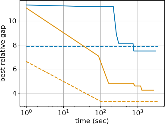
To create a warm-start initialization, we create a slightly smaller QAP by dropping the final row and column of both and (i.e. solve a size subproblem of the original instance). We use the solution to slightly smaller problem to set a warm-start initialization for the original problem, rescaling and padding with zeros where necessary. We stopped optimizing after one hour. When warm-starting, we optimize the slightly smaller problem for one hour and then optimize the original problem for one hour. Figure 2 plots the relative gap and best relative gap against time for CGAL and USBS both with and without warm-starting for one TSPLIB instance.
5.3 Interactive Entity Resolution with -constraints
Angell et al. [7] introduced a novel SDP relaxation of a combinatorial optimization problem that arises in automatic knowledge base construction [89, 51, 46]. They consider the problem of interactive entity resolution with user feedback to correct predictions made by a machine learning algorithm. Specifically, they introduce -constraints , a new paradigm of interactive feedback for correcting entity resolution predictions and presented a novel SDP relaxation as part of a heuristic algorithm for satisfying -constraints in the predicted entity resolution decisions. This novel form of feedback allows users to specify constraints stating the existence of an entity with and without certain features. As each -constraint is added to the optimization problem additional constraints are added to the SDP relaxation. We use the solution to the SDP without the newest -constraint to warm-start the solver with the new -constraint added. See Appendix E.3 for more details.
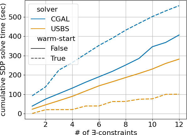
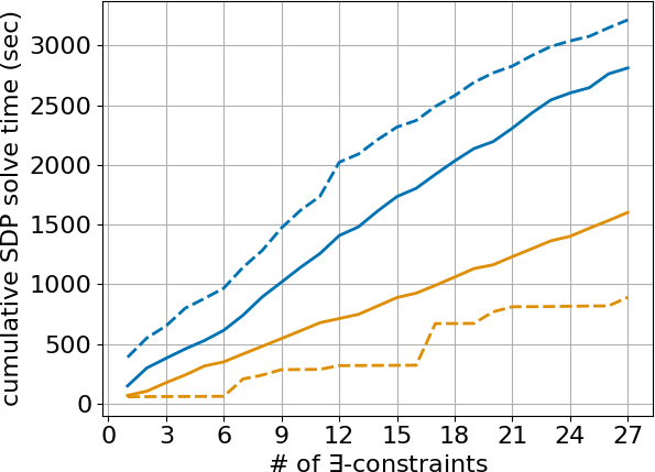
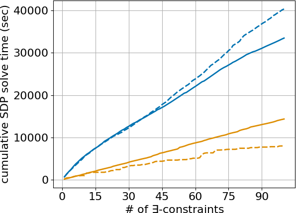
We evaluate the performance of the CGAL and USBS with and without warm-starting on the same three author coreference datasets used in [7]. In these datasets, each mention is an author-paper pair and the goal is to identify which author-paper pairs refer to the same author. We simulate -constraint generation using the same oracle implemented in [7]. Figure 3 shows the cumulative SDP solve time to reach an -approximate solution against the number of -constraints for each of the three datasets until the perfect entity resolution decsions were predicted by the inference algorithm.
| # mentions | # blocks | # clusters | nnz() | # features | |
|---|---|---|---|---|---|
| PubMed | 315 | 5 | 34 | 3,973 | 14,093 |
| QIAN | 410 | 38 | 77 | 5,158 | 10,366 |
| SCAD-zbMATH | 1,196 | 120 | 166 | 18,608 | 8,203 |
6 Related Work
Efficient SDP solving.
Due to their wide-spread applicability and importance, methods for solving SDPs efficiently have been extensively studied in the literature [84, 67, 68, 3, 18, 34, 106, 104, 29]. Interior point methods [40, 68, 3] are by far the most widely-used and well-known method for solving SDPs. Interior point methods enjoy quadratic convergence, but have incredibly high per-iteration complexity, and thus, are impractical for instances having more than a few hundred variables. ADMM [18] and splitting-based methods [69] have also been applied to solving SDPs. These methods are generally more applicable than interior point methods, but our still restricted do to the computationally expensive full eigenvalue decomposition. First-order methods such as conditional gradient augmented Lagrangian [105], primal-dual subgradient algorithms [104], the matrix multiplicative weight method [10, 88], and the mirror-prox algorithm with the quantum entropy mirror map [66] have by far the lowest per-iteration complexity among all of the methods for solving SDPs. This lower per-iteration complexity leads to slower convergence rate for these first-order methods.
Spectral bundle methods. Helmberg and Rendl [42] were the first to introduce spectral bundle methods for equality-constrained SDPs. The biggest difference between the original spectral bundle method and our approach is the model where is fixed and is chosen by the user. We find that larger provides better convergence in general and is not very helpful (and sometimes harmful) to convergence. Several other algorithmic variants of spectral bundle methods exist including solving inequality-constrained SDPs [41], trust region-based methods for nonconvex eigenvalue optimization [8], and incorporating second-order information to speed up empirical convergence [43]. Ding and Grimmer [28] present a spectral bundle method most similar to ours for solving equality-constrained SDPs. They prove an impressive set of convergence rates under various assumptions, including linear convergence if certain strong assumptions hold. The biggest difference between previous work of spectral bundle methods and USBS is the fact that USBS has more flexibility and scalability as compared with other methods both in terms of the constraints USBS supports in the SDP and the model the user can specify. In addition, this work addresses many of the practical implementation questions enabling scalability to instances with multiple orders of magnitude more variables.
Memory-efficient semidefinte programming. The most widely-known memory efficient approach to semidefinite programming is the Burer–Monteiro (BM) factorization heuristic [21]. Several optimization techniques have been used to optimize the low-rank factorized problem [98, 17, 22, 53, 74, 78]. Ding et al. [30] present an optimal storage approach to solving SDPs by first approximately solving the dual problem and then using the dual slack matrix to solve the primal problem efficiently. Yurtsever et al. [107] implement the conditional gradient augmented Lagrangian method [106] with the matrix sketching technique in [105] which forms a strong state-of-the-art method for scalably solving general SDPs. Ding and Grimmer [28] implements a spectral bundle method for solving equality constrained SDPs with the same matrix sketching technique [105].
7 Conclusion
In this work, we presented a practical spectral bundle method for solving large SDPs with both equality and inequality constraints. We proved non-asymptotic convergence rates under standard assumptions for USBS. We showed empirically that USBS is fast and scalable on practical SDP instances. Additionally, we showed that USBS can more reliably leverage a warm-start initialization to accelerate convergence. Lastly, we make our standalone implementation in pure JAX available for wide-spread use.
Acknowledgements
This work is funded in part by the Center for Data Science and the Center for Intelligent Information Retrieval at the University of Massachusetts Amherst, and in part by the National Science Foundation under grants IIS-1763618 and IIS-1922090, and in part by the Chan Zuckerberg Initiative under the project Scientific Knowledge Base Construction, and in part by IBM Research AI through the AI Horizons Network. The work reported here was performed in part by the Center for Data Science and the Center for Intelligent Information Retrieval, and in part using high performance computing equipment obtained under a grant from the Collaborative R&D Fund managed by the Massachusetts Technology Collaborative. Rico Angell is partially supported by the National Science Foundation Graduate Research Fellowship under grant 1938059. Any opinions, findings and conclusions or recommendations expressed in this material are those of the authors and do not necessarily reflect those of the sponsor(s).
References
- Agarwal et al. [2021] Dhruv Agarwal, Rico Angell, Nicholas Monath, and Andrew McCallum. Entity linking and discovery via arborescence-based supervised clustering. arXiv preprint arXiv:2109.01242, 2021.
- Agarwal et al. [2022] Dhruv Agarwal, Rico Angell, Nicholas Monath, and Andrew McCallum. Entity linking via explicit mention-mention coreference modeling. In Proceedings of the 2022 Conference of the North American Chapter of the Association for Computational Linguistics: Human Language Technologies, 2022.
- Alizadeh [1995] Farid Alizadeh. Interior point methods in semidefinite programming with applications to combinatorial optimization. SIAM journal on Optimization, 1995.
- Alizadeh et al. [1997] Farid Alizadeh, Jean-Pierre A Haeberly, and Michael L Overton. Complementarity and nondegeneracy in semidefinite programming. Mathematical programming, 1997.
- Alizadeh et al. [1998] Farid Alizadeh, Jean-Pierre A Haeberly, and Michael L Overton. Primal-dual interior-point methods for semidefinite programming: convergence rates, stability and numerical results. SIAM Journal on Optimization, 1998.
- Angell et al. [2020] Rico Angell, Nicholas Monath, Sunil Mohan, Nishant Yadav, and Andrew McCallum. Clustering-based inference for biomedical entity linking. arXiv preprint arXiv:2010.11253, 2020.
- Angell et al. [2022] Rico Angell, Nicholas Monath, Nishant Yadav, and Andrew Mccallum. Interactive correlation clustering with existential cluster constraints. In Proceedings of the 39th International Conference on Machine Learning, 2022.
- Apkarian et al. [2008] Pierre Apkarian, Dominikus Noll, and Olivier Prot. A trust region spectral bundle method for nonconvex eigenvalue optimization. SIAM Journal on Optimization, 2008.
- ApS [2019] Mosek ApS. Mosek optimization toolbox for matlab. User’s Guide and Reference Manual, Version, 2019.
- Arora et al. [2005] Sanjeev Arora, Elad Hazan, and Satyen Kale. Fast algorithms for approximate semidefinite programming using the multiplicative weights update method. In 46th Annual IEEE Symposium on Foundations of Computer Science (FOCS’05), 2005.
- [11] David A. Bader, Henning Meyerhenke, Peter Sanders, and Dorothea Wagner. Graph partitioning and graph clustering. 10th DIMACS Implementation Challenge Workshop. February 13-14, 2012. URL https://www.cise.ufl.edu/research/sparse/matrices/DIMACS10/index.html.
- Bae et al. [2020] Juhee Bae, Tove Helldin, Maria Riveiro, Sławomir Nowaczyk, Mohamed-Rafik Bouguelia, and Göran Falkman. Interactive clustering: A comprehensive review. ACM Computing Surveys (CSUR), 2020.
- Basu et al. [2010] Sumit Basu, Danyel Fisher, Steven Drucker, and Hao Lu. Assisting users with clustering tasks by combining metric learning and classification. In Proceedings of the AAAI Conference on Artificial Intelligence, volume 24, 2010.
- Beck [2015] Amir Beck. On the convergence of alternating minimization for convex programming with applications to iteratively reweighted least squares and decomposition schemes. SIAM Journal on Optimization, 2015.
- Bertsimas [1995] Dimitris Bertsimas. The achievable region method in the optimal control of queueing systems; formulations, bounds and policies. Queueing systems, 1995.
- Binette and Steorts [2022] Olivier Binette and Rebecca C Steorts. (Almost) all of entity resolution. Science Advances, 2022.
- Boumal et al. [2014] Nicolas Boumal, Bamdev Mishra, P-A Absil, and Rodolphe Sepulchre. Manopt, a matlab toolbox for optimization on manifolds. The Journal of Machine Learning Research, 2014.
- Boyd et al. [2011] Stephen Boyd, Neal Parikh, Eric Chu, Borja Peleato, Jonathan Eckstein, et al. Distributed optimization and statistical learning via the alternating direction method of multipliers. Foundations and Trends® in Machine learning, 2011.
- Bradbury et al. [2018] James Bradbury, Roy Frostig, Peter Hawkins, Matthew James Johnson, Chris Leary, Dougal Maclaurin, George Necula, Adam Paszke, Jake VanderPlas, Skye Wanderman-Milne, et al. Jax: composable transformations of python+ numpy programs. 2018.
- Bravo Ferreira et al. [2018] José FS Bravo Ferreira, Yuehaw Khoo, and Amit Singer. Semidefinite programming approach for the quadratic assignment problem with a sparse graph. Computational Optimization and Applications, 2018.
- Burer and Monteiro [2003] Samuel Burer and Renato DC Monteiro. A nonlinear programming algorithm for solving semidefinite programs via low-rank factorization. Mathematical programming, 2003.
- Burer and Monteiro [2005] Samuel Burer and Renato DC Monteiro. Local minima and convergence in low-rank semidefinite programming. Mathematical programming, 2005.
- Burkard et al. [1997] Rainer E Burkard, Stefan E Karisch, and Franz Rendl. Qaplib–a quadratic assignment problem library. Journal of Global optimization, 1997.
- Chuang and Hsu [2014] Jason Chuang and Daniel J Hsu. Human-centered interactive clustering for data analysis. In Conference on Neural Information Processing Systems (NIPS). Workshop on Human-Propelled Machine Learning, 2014.
- Coden et al. [2017] Anni Coden, Marina Danilevsky, Daniel Gruhl, Linda Kato, and Meena Nagarajan. A method to accelerate human in the loop clustering. In Proceedings of the 2017 SIAM International Conference on Data Mining, pages 237–245. SIAM, 2017.
- Dathathri et al. [2020] Sumanth Dathathri, Krishnamurthy Dvijotham, Alexey Kurakin, Aditi Raghunathan, Jonathan Uesato, Rudy R Bunel, Shreya Shankar, Jacob Steinhardt, Ian Goodfellow, Percy S Liang, et al. Enabling certification of verification-agnostic networks via memory-efficient semidefinite programming. Advances in Neural Information Processing Systems, 2020.
- Díaz and Grimmer [2023] Mateo Díaz and Benjamin Grimmer. Optimal convergence rates for the proximal bundle method. SIAM Journal on Optimization, 2023.
- Ding and Grimmer [2023] Lijun Ding and Benjamin Grimmer. Revisiting spectral bundle methods: Primal-dual (sub) linear convergence rates. SIAM Journal on Optimization, 2023.
- Ding and Udell [2021] Lijun Ding and Madeleine Udell. On the simplicity and conditioning of low rank semidefinite programs. SIAM Journal on Optimization, 2021.
- Ding et al. [2021] Lijun Ding, Alp Yurtsever, Volkan Cevher, Joel A Tropp, and Madeleine Udell. An optimal-storage approach to semidefinite programming using approximate complementarity. SIAM Journal on Optimization, 2021.
- Drusvyatskiy and Wolkowicz [2017] Dmitriy Drusvyatskiy and Henry Wolkowicz. The many faces of degeneracy in conic optimization. Foundations and Trends® in Optimization, 2017.
- Dubey et al. [2010] Avinava Dubey, Indrajit Bhattacharya, and Shantanu Godbole. A cluster-level semi-supervision model for interactive clustering. In Joint European Conference on Machine Learning and Knowledge Discovery in Databases. Springer, 2010.
- Feltenmark and Kiwiel [2000] Stefan Feltenmark and Krzysztof C Kiwiel. Dual applications of proximal bundle methods, including lagrangian relaxation of nonconvex problems. SIAM Journal on Optimization, 2000.
- Friedlander and Macedo [2016] Michael P Friedlander and Ives Macedo. Low-rank spectral optimization via gauge duality. SIAM Journal on Scientific Computing, 2016.
- Frome et al. [2007] Andrea Frome, Yoram Singer, Fei Sha, and Jitendra Malik. Learning globally-consistent local distance functions for shape-based image retrieval and classification. In 2007 IEEE 11th International Conference on Computer Vision, 2007.
- Frostig et al. [2018] Roy Frostig, Matthew James Johnson, and Chris Leary. Compiling machine learning programs via high-level tracing. Systems for Machine Learning, 2018.
- Gittens [2013] Alex Gittens. Topics in randomized numerical linear algebra. California Institute of Technology, 2013.
- Goemans and Williamson [1995] Michel X Goemans and David P Williamson. Improved approximation algorithms for maximum cut and satisfiability problems using semidefinite programming. Journal of the ACM (JACM), 1995.
- Halko et al. [2011] Nathan Halko, Per-Gunnar Martinsson, and Joel A Tropp. Finding structure with randomness: Probabilistic algorithms for constructing approximate matrix decompositions. SIAM review, 2011.
- Helmberg [1994] Christoph Helmberg. An interior point method for semidefinite programming and max-cut bounds. 1994.
- Helmberg and Kiwiel [2002] Christoph Helmberg and Krzysztof C Kiwiel. A spectral bundle method with bounds. Mathematical Programming, 2002.
- Helmberg and Rendl [2000] Christoph Helmberg and Franz Rendl. A spectral bundle method for semidefinite programming. SIAM Journal on Optimization, 2000.
- Helmberg et al. [2014] Christoph Helmberg, Michael L Overton, and Franz Rendl. The spectral bundle method with second-order information. Optimization Methods and Software, 2014.
- Hernández et al. [2007] Vicente Hernández, Jose E Román, Andrés Tomás, and Vicente Vidal. Krylov-schur methods in slepc. Universitat Politecnica de Valencia, Tech. Rep. STR-7, 2007.
- Huang et al. [2014] Qixing Huang, Yuxin Chen, and Leonidas Guibas. Scalable semidefinite relaxation for maximum a posterior estimation. In International Conference on Machine Learning. PMLR, 2014.
- Iv et al. [2022] Robert Iv, Alexandre Passos, Sameer Singh, and Ming-Wei Chang. Fruit: Faithfully reflecting updated information in text. In Proceedings of the 2022 Conference of the North American Chapter of the Association for Computational Linguistics: Human Language Technologies, 2022.
- Jonker and Volgenant [1988] Roy Jonker and Ton Volgenant. A shortest augmenting path algorithm for dense and sparse linear assignment problems. In DGOR/NSOR: Papers of the 16th Annual Meeting of DGOR in Cooperation with NSOR/Vorträge der 16. Jahrestagung der DGOR zusammen mit der NSOR. Springer, 1988.
- Karp [1972] Richard M. Karp. Reducibility among Combinatorial Problems, pages 85–103. Springer US, 1972.
- Kiwiel [2000] Krzysztof C Kiwiel. Efficiency of proximal bundle methods. Journal of Optimization Theory and Applications, 2000.
- Klein et al. [2002] Dan Klein, Sepandar D Kamvar, and Christopher D Manning. From instance-level constraints to space-level constraints: Making the most of prior knowledge in data clustering. Technical report, 2002.
- Krishnamurthy [2015] Jayant Krishnamurthy. Learning to understand natural language with less human effort. Technical report, CARNEGIE-MELLON UNIV PITTSBURGH PA SCHOOL OF COMPUTER SCIENCE, 2015.
- Kuhn [1955] Harold W Kuhn. The hungarian method for the assignment problem. Naval research logistics quarterly, 1955.
- Kulis et al. [2007] Brian Kulis, Arun C Surendran, and John C Platt. Fast low-rank semidefinite programming for embedding and clustering. In Artificial Intelligence and Statistics. PMLR, 2007.
- Kulis et al. [2009] Brian Kulis, Sugato Basu, Inderjit Dhillon, and Raymond Mooney. Semi-supervised graph clustering: a kernel approach. Machine learning, 2009.
- Lemarechal et al. [1981] Claude Lemarechal, Jean-Jacques Strodiot, and André Bihain. On a bundle algorithm for nonsmooth optimization. In Nonlinear programming 4. Elsevier, 1981.
- Li et al. [2017] Huamin Li, George C Linderman, Arthur Szlam, Kelly P Stanton, Yuval Kluger, and Mark Tygert. Algorithm 971: An implementation of a randomized algorithm for principal component analysis. ACM Transactions on Mathematical Software (TOMS), 2017.
- Li et al. [2008] Zhenguo Li, Jianzhuang Liu, and Xiaoou Tang. Pairwise constraint propagation by semidefinite programming for semi-supervised classification. In Proceedings of the 25th international conference on Machine learning, 2008.
- Li et al. [2009] Zhenguo Li, Jianzhuang Liu, and Xiaoou Tang. Constrained clustering via spectral regularization. In 2009 IEEE Conference on Computer Vision and Pattern Recognition, 2009.
- Loiola et al. [2007] Eliane Maria Loiola, Nair Maria Maia De Abreu, Paulo Oswaldo Boaventura-Netto, Peter Hahn, and Tania Querido. A survey for the quadratic assignment problem. European journal of operational research, 2007.
- Lu and Carreira-Perpinan [2008] Zhengdong Lu and Miguel A Carreira-Perpinan. Constrained spectral clustering through affinity propagation. In 2008 IEEE Conference on Computer Vision and Pattern Recognition, pages 1–8. IEEE, 2008.
- Luo and Tseng [1993] Zhi-Quan Luo and Paul Tseng. Error bounds and convergence analysis of feasible descent methods: a general approach. Annals of Operations Research, 1993.
- Mazumdar and Saha [2017] Arya Mazumdar and Barna Saha. Clustering with noisy queries, 2017.
- Mifflin [1977] Robert Mifflin. An algorithm for constrained optimization with semismooth functions. Mathematics of Operations Research, 1977.
- Mirsky [1960] Leon Mirsky. Symmetric gauge functions and unitarily invariant norms. The quarterly journal of mathematics, 1960.
- Munkres [1957] James Munkres. Algorithms for the assignment and transportation problems. Journal of the society for industrial and applied mathematics, 1957.
- Nemirovski [2004] Arkadi Nemirovski. Prox-method with rate of convergence o (1/t) for variational inequalities with lipschitz continuous monotone operators and smooth convex-concave saddle point problems. SIAM Journal on Optimization, 2004.
- Nesterov [1989] Ju E Nesterov. Self-concordant functions and polynomial-time methods in convex programming. Report, Central Economic and Mathematic Institute, USSR Acad. Sci, 1989.
- Nesterov and Nemirovskii [1994] Yurii Nesterov and Arkadii Nemirovskii. Interior-point polynomial algorithms in convex programming. SIAM, 1994.
- O’Donoghue et al. [2021] Brendan O’Donoghue, Eric Chu, Neal Parikh, and Stephen Boyd. SCS: Splitting Conic Solver, version 3.1.1. https://github.com/cvxgrp/scs, November 2021.
- Overton [1992] Michael L Overton. Large-scale optimization of eigenvalues. SIAM Journal on Optimization, 1992.
- Raghunathan et al. [2018] Aditi Raghunathan, Jacob Steinhardt, and Percy S Liang. Semidefinite relaxations for certifying robustness to adversarial examples. Advances in neural information processing systems, 2018.
- Reinelt [1995] Gerhard Reinelt. Tsplib95. Interdisziplinäres Zentrum für Wissenschaftliches Rechnen (IWR), Heidelberg, 1995. URL http://comopt.ifi.uni-heidelberg.de/software/TSPLIB95/.
- Rosen et al. [2019] David M Rosen, Luca Carlone, Afonso S Bandeira, and John J Leonard. Se-sync: A certifiably correct algorithm for synchronization over the special euclidean group. The International Journal of Robotics Research, 2019.
- Sahin et al. [2019] Mehmet Fatih Sahin, Ahmet Alacaoglu, Fabian Latorre, Volkan Cevher, et al. An inexact augmented lagrangian framework for nonconvex optimization with nonlinear constraints. Advances in Neural Information Processing Systems, 2019.
- Sato and Iwayama [2009] Yusuke Sato and Makoto Iwayama. Interactive constrained clustering for patent document set. In Proceedings of the 2nd international workshop on Patent information retrieval, pages 17–20, 2009.
- Schacke [2004] Kathrin Schacke. On the kronecker product. Master’s thesis, University of Waterloo, 2004.
- Shental et al. [2004] Noam Shental, Aharon Bar-Hillel, Tomer Hertz, and Daphna Weinshall. Computing gaussian mixture models with em using equivalence constraints. Advances in neural information processing systems, 2004.
- Souto et al. [2022] Mario Souto, Joaquim D Garcia, and Álvaro Veiga. Exploiting low-rank structure in semidefinite programming by approximate operator splitting. Optimization, 2022.
- Spielman and Srivastava [2008] Daniel A Spielman and Nikhil Srivastava. Graph sparsification by effective resistances. In Proceedings of the fortieth annual ACM symposium on Theory of computing, 2008.
- Sremac et al. [2021] Stefan Sremac, Hugo J Woerdeman, and Henry Wolkowicz. Error bounds and singularity degree in semidefinite programming. SIAM Journal on Optimization, 2021.
- Sturm [1999] Jos F Sturm. Using SeDuMi 1.02, a matlab toolbox for optimization over symmetric cones. Optimization methods and software, 1999.
- Sturm [2000] Jos F Sturm. Error bounds for linear matrix inequalities. SIAM Journal on Optimization, 2000.
- Subramanian et al. [2021] Shivashankar Subramanian, Daniel King, Doug Downey, and Sergey Feldman. S2AND: A Benchmark and Evaluation System for Author Name Disambiguation. In Proceedings of the ACM/IEEE Joint Conference on Digital Libraries in 2021, 2021.
- Todd [2001] Michael J Todd. Semidefinite optimization. Acta Numerica, 2001.
- Todd et al. [1998] Michael J Todd, Kim-Chuan Toh, and Reha H Tütüncü. On the nesterov–todd direction in semidefinite programming. SIAM Journal on Optimization, 1998.
- Toh et al. [1999] Kim-Chuan Toh, Michael J Todd, and Reha H Tütüncü. Sdpt3—a matlab software package for semidefinite programming, version 1.3. Optimization methods and software, 1999.
- Tropp et al. [2017] Joel A Tropp, Alp Yurtsever, Madeleine Udell, and Volkan Cevher. Fixed-rank approximation of a positive-semidefinite matrix from streaming data. Advances in Neural Information Processing Systems, 2017.
- Tsuda et al. [2005] Koji Tsuda, Gunnar Rätsch, and Manfred K Warmuth. Matrix exponentiated gradient updates for on-line learning and bregman projection. Journal of Machine Learning Research, 2005.
- Uhlen et al. [2010] Mathias Uhlen, Per Oksvold, Linn Fagerberg, Emma Lundberg, Kalle Jonasson, Mattias Forsberg, Martin Zwahlen, Caroline Kampf, Kenneth Wester, Sophia Hober, et al. Towards a knowledge-based human protein atlas. Nature biotechnology, 2010.
- Vandenberghe and Boyd [1999] Lieven Vandenberghe and Stephen Boyd. Applications of semidefinite programming. Applied Numerical Mathematics, 1999.
- Vandenberghe et al. [1998a] Lieven Vandenberghe, Stephen Boyd, and Abbas El Gamal. Optimizing dominant time constant in RC circuits. IEEE Transactions on Computer-Aided Design of Integrated Circuits and Systems, 1998a.
- Vandenberghe et al. [1998b] Lieven Vandenberghe, Stephen Boyd, and Shao-Po Wu. Determinant maximization with linear matrix inequality constraints. SIAM journal on matrix analysis and applications, 1998b.
- Vikram and Dasgupta [2016] Sharad Vikram and Sanjoy Dasgupta. Interactive bayesian hierarchical clustering. In International Conference on Machine Learning, 2016.
- Viswanathan et al. [2023] Vijay Viswanathan, Kiril Gashteovski, Carolin Lawrence, Tongshuang Wu, and Graham Neubig. Large language models enable few-shot clustering. arXiv preprint arXiv:2307.00524, 2023.
- Wagstaff and Cardie [2000] Kiri Wagstaff and Claire Cardie. Clustering with instance-level constraints. AAAI/IAAI, 2000.
- Wagstaff et al. [2001] Kiri Wagstaff, Claire Cardie, Seth Rogers, Stefan Schrödl, et al. Constrained k-means clustering with background knowledge. In Icml, 2001.
- Waldspurger and Waters [2020] Irene Waldspurger and Alden Waters. Rank optimality for the burer–monteiro factorization. SIAM journal on Optimization, 2020.
- Wang et al. [2017] Po-Wei Wang, Wei-Cheng Chang, and J Zico Kolter. The mixing method: low-rank coordinate descent for semidefinite programming with diagonal constraints. arXiv preprint arXiv:1706.00476, 2017.
- Wu et al. [1999] Kesheng Wu, Andrew Canning, HD Simon, and L-W Wang. Thick-restart lanczos method for electronic structure calculations. Journal of Computational Physics, 1999.
- Xing et al. [2002] Eric Xing, Michael Jordan, Stuart J Russell, and Andrew Ng. Distance metric learning with application to clustering with side-information. Advances in neural information processing systems, 2002.
- Xiong et al. [2016] Caiming Xiong, David M Johnson, and Jason J Corso. Active clustering with model-based uncertainty reduction. IEEE transactions on pattern analysis and machine intelligence, 2016.
- Yadav et al. [2021] Nishant Yadav, Nicholas Monath, Rico Angell, and Andrew McCallum. Event and entity coreference using trees to encode uncertainty in joint decisions. In Proceedings of the Fourth Workshop on Computational Models of Reference, Anaphora and Coreference, 2021.
- Yang et al. [2015] Liuqin Yang, Defeng Sun, and Kim-Chuan Toh. Sdpnal+: a majorized semismooth newton-cg augmented lagrangian method for semidefinite programming with nonnegative constraints. Mathematical Programming Computation, 2015.
- Yurtsever et al. [2015] Alp Yurtsever, Quoc Tran Dinh, and Volkan Cevher. A universal primal-dual convex optimization framework. Advances in Neural Information Processing Systems, 2015.
- Yurtsever et al. [2017] Alp Yurtsever, Madeleine Udell, Joel Tropp, and Volkan Cevher. Sketchy decisions: Convex low-rank matrix optimization with optimal storage. In Artificial intelligence and statistics. PMLR, 2017.
- Yurtsever et al. [2019] Alp Yurtsever, Olivier Fercoq, and Volkan Cevher. A conditional-gradient-based augmented lagrangian framework. In International Conference on Machine Learning, 2019.
- Yurtsever et al. [2021] Alp Yurtsever, Joel A Tropp, Olivier Fercoq, Madeleine Udell, and Volkan Cevher. Scalable semidefinite programming. SIAM Journal on Mathematics of Data Science, 2021.
- Zaslavskiy et al. [2008] Mikhail Zaslavskiy, Francis Bach, and Jean-Philippe Vert. A path following algorithm for the graph matching problem. IEEE Transactions on Pattern Analysis and Machine Intelligence, 2008.
- Zhao et al. [1998] Qing Zhao, Stefan E Karisch, Franz Rendl, and Henry Wolkowicz. Semidefinite programming relaxations for the quadratic assignment problem. Journal of Combinatorial Optimization, 1998.
Appendix A Derivations
A.1 Penalized Dual Objective
Begin by considering the following Lagrangian formulation of the model problem
| (22) |
where the Lagrangian is defined as
| (23) |
Since , we know
| (24) |
Furthermore, it is easy to show the following fact [70],
| (25) |
Incorporating (25) with (24) allows us to write an equivalent formulation of the original dual problem by defining the penalized dual objective as shown in (pen-D)
| (pen-D) |
where is the indicator function defined such that if and otherwise.
A.2 Equivalent Penalized Dual Objective
A.3 Candidate Iterate
Notice that the candidate iterate can be written as follows
| (27) |
where
To solve for , start by fixing arbitrarily. Then, completing the square gives
This implies that the candidate iterate can be computed as follows
| (28) |
where is the solution to the following optimization problem
| (29) |
where
| (30) |
Appendix B Solving Iteration Subproblems
In this section, we detail the primal-dual path-following interior point methods used to solve the small semidefinite program to compute the value and the small quadratic semidefinite program (16). Before we can derive the algorithms, it is necessary to define the operator and symmetric Kronecker product [5, 76, 85].
For any matrix , the vector is defined as
The -operator is a structure preserving map between and where the constant multiplied by some of the entries ensures that
For any , let be the map from to defined by stacking the columns of into a single -dimensional vector. It is also useful to define the matrix which maps for any . Let be the entry in the row which defines element in and the column that is multiplied with the element in . Then
As an example, the case when :
Note that is a unique matrix with orthonormal rows and has the following property
The symmetric Kronecker product can be defined for any two square matrices by its action on a vector for as follows
Alternatively, but equivalently [76], the symmetric Kronecker product can be defined more explicitly using the matrix defined above as follows
where is the standard Kronecker product. We use this latter definition in our implementation.
B.1 Computing
The value is the optimum value of the following optimization problem (remember that can be dropped since is always feasible)
This amounts to computing where is a solution to the following (small) semidefinite program
| (31) | ||||
where
We will use a primal-dual interior point method to solve (31). We follow the well known technique for deriving primal-dual interior point methods [40]. We start by defining the Lagrangian of the dual barrier problem of (31),
| (32) | ||||
where we introduce a dual slack matrix as complementary to , a dual slack scalar as complementary to , a Lagrange multiplier for the trace constraint inequality, and a barrier parameter . Notice that we have moved from needing to optimize a constrained optimization problem to an unconstrained optimization problem. The saddle point solution of (32) is given by the solution of the KKT-conditions, which reduces to just the first-order optimality conditions since the problem is unconstrained. The first-order optimality conditions of (32) are the following system of equations
| (33) | ||||
| (34) | ||||
| (35) | ||||
| (36) | ||||
| (37) |
By the strict concavity of , , and , there exists a unique solution to this system of equations for any value of the barrier parameter . The sequence of these solutions as forms the central trajectory (also known as the central path). For a point on the central trajectory, we can use any combination of (35), (36), and/or (37) to solve for ,
| (38) |
The fundamental idea of primal-dual interior point methods is to use Newton’s method to follow the central path to a solution of (31). Before we can apply Newton’s method, we must linearize the non-linear equations (35), (36), and (37) into an equivalent linear formulation. There are several ways one could linearize these equations and the choice of linearization significantly impacts the algorithm’s behavior (see [5] or [40] for more on the choice of linearization). We choose one standard method linearization, detailed in the following system of equations
| (39) |
The solution to this system of equations satisfies the first-order optimality conditions (33)-(37) and is the optimal solution to the barrier problem. We utilize Newton’s method to take steps in the update direction towards . The update direction determined by Newton’s method must satisfy the following equation
Hence, the update direction is the solution to the following system of equations (after the same standard linearization has been applied to the following system as in (39))
| (40) | ||||
| (41) | ||||
| (42) | ||||
| (43) | ||||
| (44) |
We can solve this system efficiently by analytically eliminating all variables except . We can compute by solving the following linear matrix equation using an off-the-shelf linear system solver
| (45) | ||||
where . Then, computing the rest of the update directions , , , and amounts to back-substituting the solution to (45) for through the analytical variable elimination equations.
Given how to compute the update directions, the primal-dual interior point method proceeds as follows. Initialize the variables to an arbitrary strictly feasible point (i.e. , , , , and ). Starting from this primal-dual pair we compute an estimate of the barrier parameter as follows
where, as done in [40], we use (38) and divide by two. Then, we compute the update direction as described above and perform a backtracking line search to find a step size such that is again strictly feasible. Lastly, following [42], we compute a non-increasing estimate of the barrier parameter
We iterate over these steps until the barrier parameter is small enough (e.g. ).
B.2 Solving (16)
The subproblem (16) can be rewritten as the following (small) quadratic semidefinite program
For this subproblem, unlike the subproblem solved in subsection B.1, we are solving for and to compute the candidate iterate , update the primal variable, and update the model. This (small) quadratic semidefinite program is equivalent to the following optimization problem
| (46) | ||||
where
We follow the same derivation procedure as in subsection B.1, so we proceed by including the details which differ from the previous section. The Lagrangian of the dual barrier problem of (46) is as follows
| (47) | ||||
The first-order optimality conditions of (47) yields the following system of equations (after the same standard linearization)
| (48) |
The Newton’s method step direction is determined via the following linearized system
| (49) | ||||
| (50) | ||||
| (51) | ||||
| (52) | ||||
| (53) |
We can solve this system efficiently by analytically eliminating all variables except . We can compute by solving the following linear matrix equation using an off-the-shelf linear system solver
| (54) | ||||
where and . Then, computing the rest of the update directions , , , and amounts to back-substituting the solution to (54) for through the analytical variable elimination equations.
We make a single change to the initialization as compared with the interior point method presented in subsection B.1. Since this interior point method can be executed multiple times in a row with only the value of changing as the first step in the alternating maximization algorithm, we warm-start initialize with the previous execution’s . We observe non-negligible convergence improvements over arbitrary initialization as this interior point method procedure is called in sequence.
B.3 Remark on Solving Subproblems
Ding and Grimmer [28] claim that (16) could be solved using (accelerated) projected gradient descent and describe the method necessary for projection and proper scaling, but they use Mosek [9], an off-the-shelf solver, in their experiments. We find that while theoretically possible, projected gradient descent does not work well in practice since choosing the correct step size to obtain a high quality solution to (16) is difficult and varies between time steps . We instead use (and advocate for) the primal-dual interior point method derived in Appendix B.2.
Appendix C Additional Details on Scaling with Matrix Sketching
The values , , and can be efficiently maintained given low-rank updates to due to the linearity of the operations,
| (55) | ||||
| (56) | ||||
| (57) |
where can be computed efficiently since
| (58) |
C.1 Nyström Sketch Reconstruction
Given the sketch and the projection matrix , we can compute a rank- approximation to . The approximation is as follows
| (59) |
where is the Moore-Penrose inverse. The reconstruction is called a Nyström approximation. We will almost always compute the best rank- approximation of for memory efficiency. In practice, we use the numerically stable implementation of the Nyström approximation provided by Yurtsever et al. [107]. The Nyström approximation yields a provably good approximation for any sketched matrix. See the following fact from [87],
Fact C.1.
Fix arbitrarily. Let where has independently sampled standard normal entries. For each , the Nyström approximation as defined in (59) satisfies
| (60) |
where is the expectation with respect to and is returns an -truncated singular-value decomposition of the matrix , which is a best rank-r approximation with respect to every unitarily invariant norm [64]. If we replace with , this error bound still remains valid.
C.2 USBS Memory Requirements.
When we implement USBS using this matrix sketching procedure we see significant decrease in time and memory required by USBS. Storing the projection matrix and requires memory. Storing and requires memory, respectively, and storing , , , and requires memory. The primal-dual interior point methods require and memory, respectively, and storing requires memory. This means that the entire memory required by USBS is working memory (not including the memory to store the problem data) which for many SDPs is much less than explicitly storing the iterate which requires memory.
Appendix D Proof of Theorem 3.1
In this section, we present the non-asymptotic convergence results for USBS. First, we summarize the relevant results presented by Díaz and Grimmer [27] in the following theorem.
Theorem D.1.
Let and be constant, be a proper closed convex function with nonempty set of minimizers , and the sequence of models produced by the proximal bundle method satisfy the conditions (3), (4), and (5). If the iterates and subgradients are bounded, then the iterates have for all . Additionally, if for all , then the bound improves to for all .
We will use this result to prove the non-asymptotic convergence rates for the spectral bundle method.
Note the following fact necessary to use Theorem D.1.
Fact D.2.
The set is compact and contains all iterates . Moreover, the iterates and subgradients are bounded, i.e. and .
Proof.
The function is continuous and proper over the domain . It is a well-known fact that the level sets of continuous proper functions are compact. Hence, the union of level sets is compact, and therefore, . The subgradients take the form where is a unit-normed vector, and thus, for all . ∎
The following lemma guarantees quadratic growth whenever strict complementarity holds.
Lemma D.3.
Proof.
The following three lemmas guarantee primal feasiblity, dual feasibility, and primal-dual objective optimality given convergence of the penalized dual objective, i.e. .
Lemma D.4.
At every descent step ,
| (62) |
Additionally, if Slater’s condition holds and is unique, then
| (63) |
Proof.
Lemma D.5.
Suppose strong duality holds and . Then, at every descent step ,
| (64) |
Proof.
By definition of strong duality, we know that for any that , and equivalently, . Then, the dual objective gap is bounded as follows
We now utilize this bound to obtain the desired result
where the last inequality is implied by the assumption that .
∎
Lemma D.6.
At every descent step ,
| (65) |
Additionally, if Slater’s condition holds and is unique, then
| (66) |
Proof.
We start by rewriting the primal-dual gap as follows
We will now bound the absolute values of the two resulting terms to bound the desired quantity. Using the Cauchy-Schwarz inequality and Lemma D.4 it can be seen
where the last inequality comes from Fact D.2. Assume Slater’s condition holds and is unique. Then, using Lemma D.3 gives
Since and by construction, we can use Lemma D.5 to yield
The immediately yields the desired result. ∎
D.1 Proof of Theorem 3.1
The overall proof strategy is to use Theorem D.1 to show that the penalized dual gap, , converges at a worst case rate of , which improves to if Slater’s condition or strict complementarity hold. Then, we can use Lemmas D.4, D.5, and D.6 to obtain the stated convergence of primal feasibility, dual feasibility, and primal-dual optimality.
To apply the result of Theorem D.1, we showed that the norms of the iterates and subgradients of are bounded (Fact D.2), and so all we need to do is show that the model satisfies the conditions (3), (4), and (5).
Let be a maximum eigenvector if and , otherwise. Then denote as the subgradient of corresponding at the candidate iterate . Let be the aggregate subgradient. Recall that at iteration the model approximates by the low-dimensional spectral set
and therefore the penalized dual objective and model respectively take the following forms for any ,
| (67) |
Verifying (3).
Verifying (4).
Since spans , there exists a vector such that . Taking and implies . Hence,
Verifying (5).
From the first-order optimality conditions and the update step (14) we know that
To show the desired result, we first want to show that . If , we are done since . Otherwise, . First note that by construction. Then,
Since spans each of the columns of , we can conclude that . Thus, for any ,
Appendix E Experimental Setup and Details
Following [107], we scale the problem data for all problems such that the following condition holds,
| (68) |
In all three problem types, the constraints exactly determine the trace of all optimal solutions. Since we know the trace of the optimal solution and we apply problem scaling (68), we can set for all problem types.
Computing the relative infeasibility is simple. As for the relative primal objective suboptimality, we do not usually have access to the optimal primal objective value , but we can compute an upper bound. For any ,
| (69) | ||||
We use this upper bound to approximate the relative primal objective suboptimality in our experiments for USBS. We use the upper bound given in [107] to compute the relative primal objective suboptimality for CGAL.
For both CGAL and USBS, we compute eigenvectors and eigenvalues using an implementation of the thick-restart Lanczos algorithm [99, 44] with 32 inner iterations and a maximum of 10 restarts. Both CGAL and USBS are implemented using 64-bit floating point arithmetic. Unless otherwise specified, we use a CPU machine with 16 cores and up to 128 GB of RAM. Throughout the presentation of the experimental results we use to indicate that higher is better for that particular metric and to indicate lower is better for that particular metric.
E.1 MaxCut
The MaxCut problem is a fundamental combinatorial optimization problem and its SDP relaxation is a common test bed for SDP solvers. Given an undirected graph, the MaxCut is a partitioning of the vertices into two sets such that the number of edges between the two subsets is maximized. Formally, the MaxCut problem can be written as follows
| (70) |
where is the graph Laplacian. This optimization problem is known to be NP-hard [48], but rounding the solution to the SDP relaxation can yield very strong approximate solutions [38].
E.1.1 SDP Relaxation
For any vector , the matrix is positive semidefinite and all of its diagonal entries are exactly one. These implicit constraints allow us to arrive at the MaxCut SDP as follows
| (71) |
where extracts the diagonal of a matrix into a vector and is the all-ones vector. A matrix solution to (20) does not readily elicit a graph cut. One way to round is to compute a best rank-one approximation and use as an approximate cut. There are more sophisticated rounding procedures (e.g. [38]), but this one works quite well in practice.
Notice that (20) contains exactly equality constraints. Additionally, in many instances of MaxCut, the graph Laplacian is sparse and the optimal solution is low-rank. This means that we can represent the MaxCut instance with far less than memory. These attributes make sketching the matrix variable with relatively small an attractive and effective approach when considering the MaxCut problem.
E.1.2 Rounding
Both CGAL and USBS maintain a sketch of the primal variable that, along with the test matrix, can be used to construct a low-rank approximation of the primal iterate where has orthonormal columns. Following [107], we evaluate the size of cuts given by the column vectors of and choose the largest.
E.1.3 Experimental Setup
We evaluate the CGAL and USBS with and without warm-starting on ten instances from the DIMACS10 [11] where and the number of edges in each graph are shown in Table 1. We warm-start each method by dropping the last 1% of vertices from the graph resulting in a graph with 99% of the vertices. We pad the solution from the 99%-sized problem with zeros and rescale as necessary to create the warm-start initialization. Unless otherwise specified, we use the following hyperparameters for USBS in our experiments: , , , , . In our experiments, we find that does improve performance slightly. See the implementation for more details.
E.2 Quadratic Assignment Problem
The quadratic assignment problem (QAP) is a very difficult but fundamental class of combinatorial optimization problems containing the traveling salesman problem, max-clique, bandwidth problems, and facilities location problems among others [59]. SDP relaxations have been shown to facilitate finding good solutions to large QAPs [109]. The QAP can be formally defined as follows
| (72) |
where is the weight matrix, is the distance matrix, and the goal is to optimize for an assignment which aligns and . The number of permutation matrices is , so a brute-force search becomes quickly intractable as n grows. Generally, QAP instances with are intractable to solve exactly. In our experiments, using an SDP relaxation and rounding procedure, we can obtain good solutions to QAPs where n is between 136 and 198.
E.2.1 SDP Relaxation
There are many SDP relaxtions for QAPs, but we consider the one presented by [107] and inspired by [45, 20] which is formulated as follows
| (73) | ||||
where denotes the Kronecker product, and denote the partial trace over the first and second systems of Kronecker product respectively, extracts the entries of Y corresponding to the nonzero entries of , and stacks the columns of a matrix one on top of the other to form a vector. In many cases, one of or is sparse (i.e. nonzero entries) resulting in total constraints for the SDP.
The primal variable has dimension and as a result the SDP relaxation has decision variables. Given the aggressive growth in complexity, most SDP based algorithms have difficulty operating on instances where . To reduce the number of decision variables, we sketch with , resulting in entries in the sketch and the same number of constraints in most natural instances. We show that this enables CGAL and USBS to scale to instances where (more than 1.5 billion decision variables and constraints).
E.2.2 Rounding
We adopt the rounding method presented in [107] to convert an approximate solution of (21) into a permutation matrix. Reconstructing an approximation to the primal variable from the sketch yields where has shape . For each column of , we discard the first entry of the column vector, reshape the remaining entries into an matrix, and project the reshaped matrix onto the set of permutation matrices using the Hungarian method (also known as Munkres’ assignment algorithm) [52, 65, 47]. This procedure yields a feasible point to the original QAP (72). To get an upper bound for (72), we perform the rounding procedure on each column of and choose the permutation matrix which minimizes the objective .
E.2.3 Experimental Setup
We evaluate CGAL and USBS on select large instances from QAPLIB [23] and TSPLIB [72] ranging in size from 136 to 198. Provided with each of these QAP instances is the known optimum. For many instances, we find that the quality of the permutation matrix produced by the rounding procedure does not entirely correlate with the quality of the iterates with respect to the SDP (21). Thus, we apply the rounding procedure at every iteration of both CGAL and USBS. Our metric for evaluation is relative gap which is computed as follows
We report the lowest value so far of relative gap as best relative gap. CGAL [107] is shown to obtain significantly smaller best relative gap than CSDP [20] and PATH [108] on most instances, and thus, is a strong baseline.
To create a warm-start initialization, we create a slightly smaller QAP by dropping the final row and column of both and (i.e. solve a size subproblem of the original instance). We use the solution to slightly smaller problem to set a warm-start initialization for the original problem, rescaling and padding with zeros where necessary. We stopped optimizing after one hour. When warm-starting, we optimize the slightly smaller problem for one hour and then optimize the original problem for one hour.
E.3 Interactive Entity Resolution with -constraints
Angell et al. [7] introduced a novel SDP relaxation of a combinatorial optimization problem that arises in an automatic knowledge base construction problem [89, 51, 46]. They consider the problem of interactive entity resolution with user feedback to correct predictions made by a machine learning algorithm. Entity resolution (also known as coreference resolution or record linkage) is the process of identifying which mentions (sometimes referred to as records) of entities refer to the same entity [16, 6, 1, 2, 102]. Entity resolution is an important problem central to automated knowledge base construction where the correctness of the resulting knowledge base is vital to its usefulness. The entity resolution problem is fundamentally a clustering problem where the prefect clusters contain all mentions of exactly one entity. Due to the large volumes of raw data frequently involved, machine learning approaches are often used to perform entity resolution. To correct inevitable errors in the predictions made by these automated methods, human feedback can be used to correct errors in entity resolution.
Utilizing human feedback to guide and correct clustering decisions can be broadly categorized into two groups [12]: active clustering (also know as semi-supervised clustering) [94, 93, 62, 75, 101] and interactive clustering [24, 13, 25, 32]111Commonly, active clustering is used to describe techniques where the algorithm queries the human for feedback about a specific pair or group of points or clusters (akin to active learning) and interactive clustering is used to describe techniques where humans observe the clustering output and provide unelicited feedback, typically in the form of some type of constraint, to the algorithm.. There are several paradigms of human feedback used to steer a clustering algorithm [35, 96, 77, 50, 54, 60, 57, 58, 100], the most common of which is pairwise constraints [95] (i.e. statements about whether two points or mentions must or cannot be clustered together). Recently, Angell et al. [7] introduced -constraints , a new paradigm of interactive feedback for correcting entity resolution predictions and presented a novel SDP relaxation as part of a heuristic algorithm for satisfying -constraints in the predicted clustering. This novel form of feedback allows users to specify constraints stating the existence of an entity with and without certain features.
E.3.1 -constraints
To define -constraints precisely, we must introduce some terminology and notation. Let the set of mentions be represented by the vertex set of a fully connected graph. We assume that each of the mentions has an associated set of discrete features (attributes, relations, other features, etc.) that is readily available or can be extracted easily using some automated method. Let be the set of possible features and be the subset of features associated with vertex . A clustering of vertices is a set of nonempty sets such that , for all , and . We denote the ground truth clustering of the vertices (partitioning mentions into entities) as . Furthermore, for any subset of vertices , we define the set of features associated with as . For any cluster , we use as the canonicalization function for a predicted entity, but this framework allows for more complex (and even learned) canonicalization functions. When providing feedback, users are able to view the features of predicted clusters and then provide one or more -constraints .
Formally, a -constraint uniquely characterizes a constraint asserting there exists a cluster such that all of the positive features are contained in the features of (i.e. ) and none of the negative features are contained in the features of (i.e. ). At any given time, let the set of -constraints be represented by . We say that a subset of nodes satisfies a -constraint if and . Note that more than one ground truth cluster can satisfy a -constraint . We say that a subset of vertices is incompatible with a -constraint if and denote this as . Similarly, two -constraints are incompatible if or , and is also denoted . Furthermore, we say a subset of vertices and a -constraint or two -constraints are compatible if they are not incompatible and denote this as and , respectively. Moreover, we use compatible to describe when a subset of vertices could be part of a cluster that satisfies a certain -constraint . This definition allows for to be empty, but still enables to be compatible with just as long as is empty. Observe that if every mention has a unique feature, the -constraint framework fully encompasses must-link and cannot-link constraints.
E.3.2 SDP relaxation
Following [7], the general approach to clustering with -constraints is to jointly cluster the vertices and the -constraints , so we include -constraints as additional vertices of the graph (i.e. ) and create corresponding decision variables for each of the -constraints . Additionally, we create constraints to ensure that all of the -constraints are satisfied and none of the -constraints are incompatible with any of the other members of the predicted clustering. Given a -constraint and positive feature , let be the set of candidate vertices that could satisfy . The resulting integer linear programming problem is as follows
| (75) |
where is the pairwise similarity between mentions and (usually computed using a trained machine learning model trained on pairs of mentions) and is the standard basis vector. Note that we assume that the as in [7]. The first constraint ensures that all of the positive features in are contained in the same cluster as for all . The last constraint ensures that is not in the same cluster as anything incompatible with it for all . This problem is intractable to optimize exactly, so we relax (75) to an SDP in the standard way as follows
| (76) |
The decision variables are changed from standard basis vectors, whose dot products determine whether or not two elements (vertices or -constraints ) are in the same cluster, to a positive semidefinite matrix where each entry represents the global affinity two elements have for one another (corresponding to the row and column of the entry). We constrain the diagonal of this positive semidefinite matrix to be all ones (representing each element’s affinity with itself) and we enforce that all entries in the matrix are non-negative. The constraints ensuring -constraint satisfaction are similar to (75). Let be the (weighted) adjacency matrix of the fully connected graph over the vertices.
E.3.3 Rounding
The solution to (76) is a fractional approximation of the problem we wish to solve. In order to infer a predicted clustering, we need some procedure to round the fractional solution to an integer solution. Angell et al. [7] propose first building a hierarchical clustering over using as the similarity function. Then, a dynamic programming algorithm is used to extract a (predicted) flat clustering from the hierarchical clustering which maximizes the number -constraints satisfied and the (correlation) clustering objective. For a more detailed description of the rounding procedure, see [7]. The predicted clustering is then observed by the human users in terms of the features of each predicted cluster enabling the users to provide any additional -constraints to correct the entity resolution decisions. We simulate this human feedback loop with an oracle -constraint generator.
E.3.4 Experimental Setup
We evaluate the performance of the CGAL and USBS with and without warm-starting on the same three author coreference datasets used in [7]. In these datasets, each mention is an author-paper pair and the goal is to identify which author-paper pairs were written by the same author. As standard in author coreference, the datasets are preprocessed into blocks (also known as canopies) based on the author’s first name initial and last name (e.g. authors “Rajarshi Das” and “Ravi Das” would both be contained in the same block “r das”, but in a different block than “Jane Smith”, which would be in “j smith”). Within each block, similarity scores are computed between all pairs of mentions using a trained pairwise model [7, 83]. We then perform two additional preprocessing steps to convert the many small dense problems into one large sparse problem. We aggregate all of these pairwise similarity scores into a block diagonal weight matrix and fill the remaining entries with negative one. We then sparsify this highly structured similarity matrix using a spectral sparsifier [79]. Table 3 details the dataset statistics including the number of non-zeros in the pairwise similarity matrix after spectral sparsification, denoted nnz().
| # mentions | # blocks | # clusters | nnz() | # features | |
|---|---|---|---|---|---|
| PubMed | 315 | 5 | 34 | 3,973 | 14,093 |
| QIAN | 410 | 38 | 77 | 5,158 | 10,366 |
| SCAD-zbMATH | 1,196 | 120 | 166 | 18,608 | 8,203 |
We simulate -constraint generation using the same oracle implemented in [7]. The oracle has access to the features of the ground truth clusters and the features of the predicted clusters output by the rounding algorithm and generates a small -constraint which is satisfied by the ground truth clustering, but is not satisfied by the predicted clustering. The oracle generates -constraints one at a time and added to the optimization problem until the ground truth clustering is predicted. For both solvers, we iterate until the relative error tolerance (19) and the following absolute infeasibility condition are satisfied
| (77) |
We use to determine the stopping condition and find that this is sufficient for the rounding algorithm to satisfy nearly all of the -constraints generated by the oracle. We also note that the -norm condition is especially important in this application in order to make sure the relaxed -constraints are satisfied. Due to the small problem size, we simplify the implementation by using variants of CGAL and USBS without sketching.
When warm-starting, we predict the values of the expanded primal variable corresponding to the newly added -constraint by computing representations of each vertex using a low-rank factorization, performing a weighted average of the representations of the positive vertices in the newly added -constraint , and expanding the factorization into an initialization of primal variable for the new problem. We pad the dual variable with zeros. Since there is no pairwise similarity between -constraints and mentions, we find that scaling up the norms of ’s corresponding to the constraints for all such that , where is the newly added -constraint . We use the following USBS hyperparameters in our experiments: , , , . See the implementation for more details.
Appendix F Additional Experimental Results
F.1 MaxCut
Figure 4 plots three different convergence measures over time for a large data instance, 144, for a total time of 12 hours. For this instance, warm-starting helps achieve a faster convergence rate of both relative primal objective suboptimality and relative infeasibility. Additionally, the weight of the cut produced from the primal iterates generated by USBS drops in value less when warm-starting as compared with CGAL. This is an additional indication that USBS is able to utilize the warm-start initialization better than CGAL. Finally, observe that USBS, with and without warm-starting, produces a marginally better graph cut than CGAL.
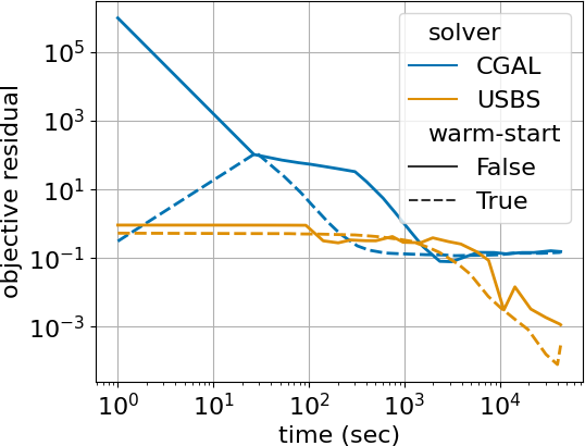
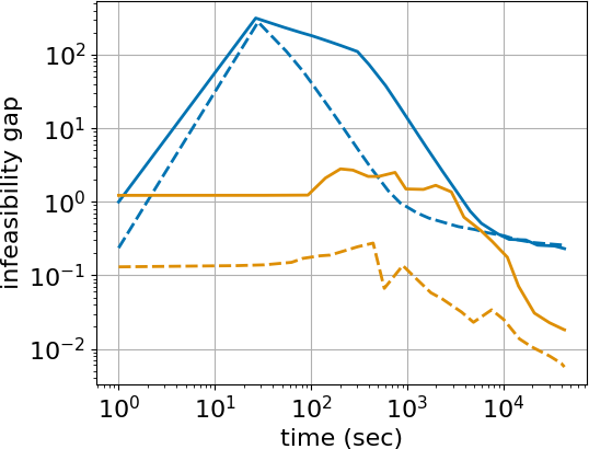
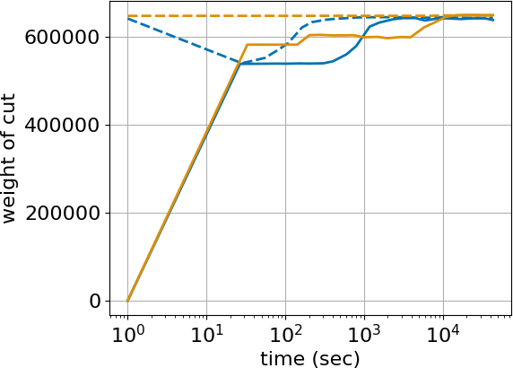
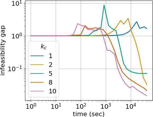
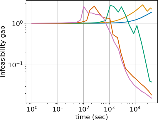
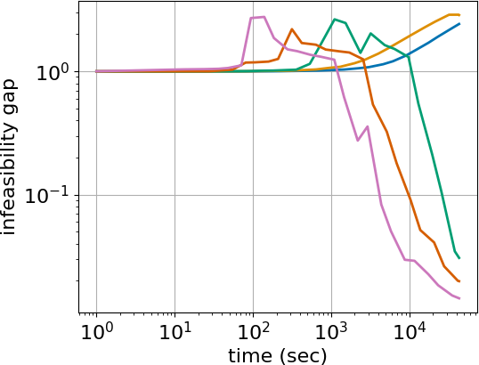
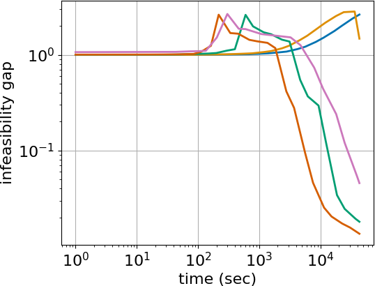
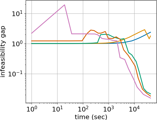
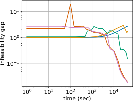
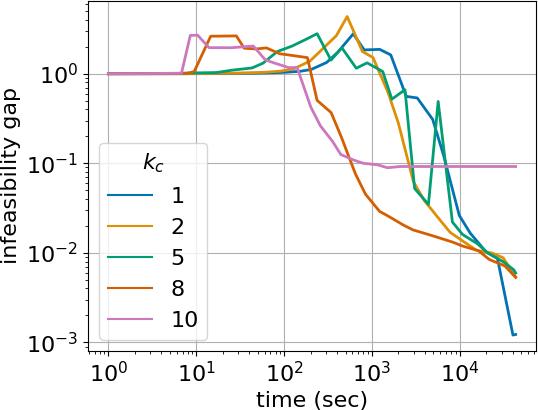
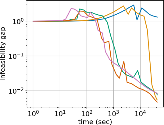
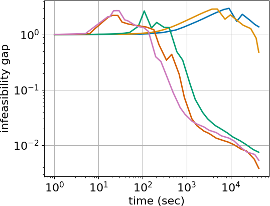
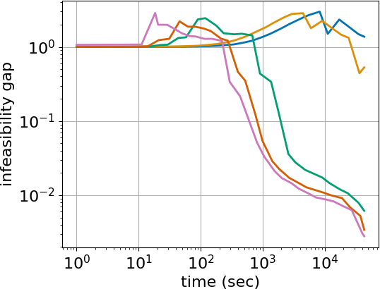
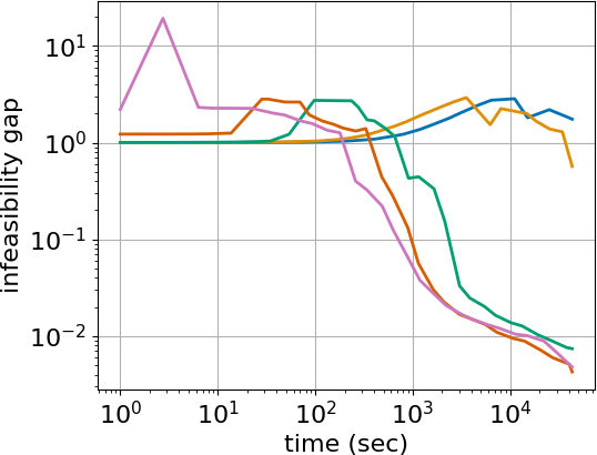
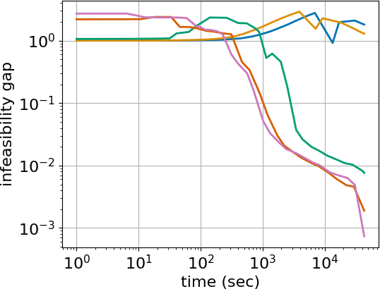
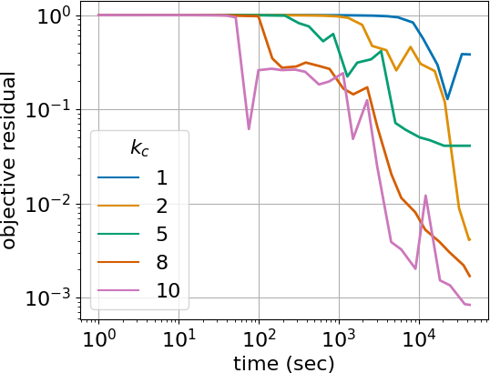
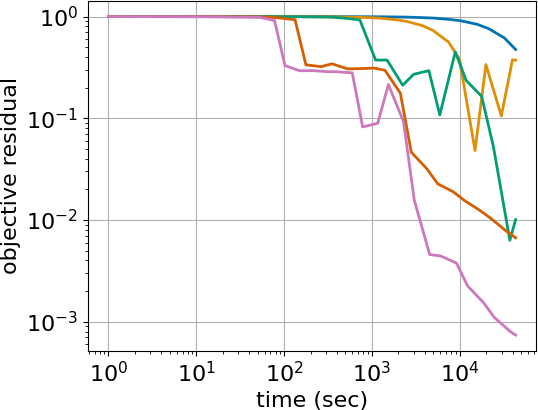
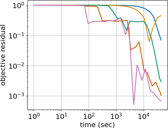
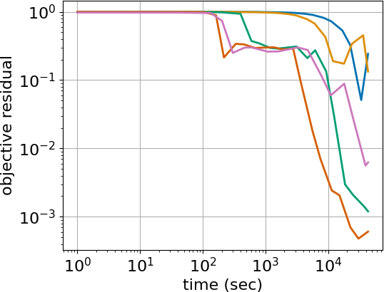
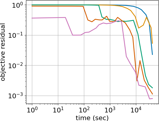
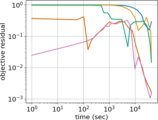
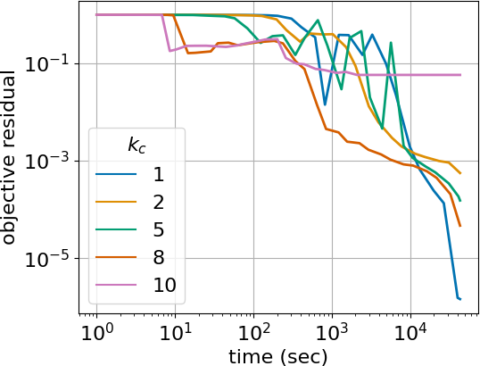
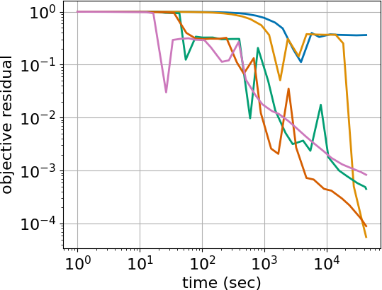
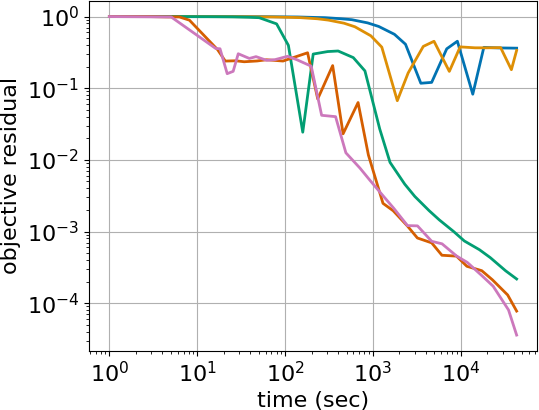
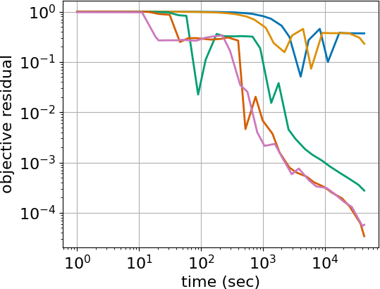
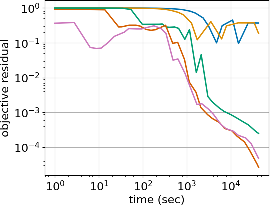
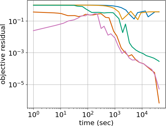
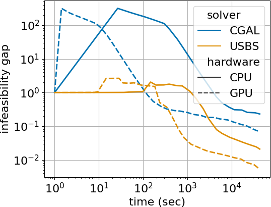
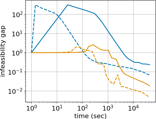
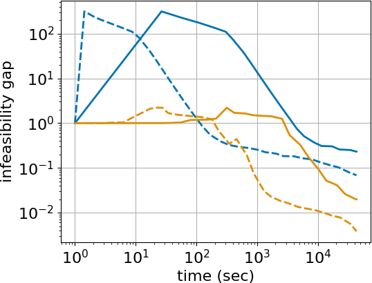
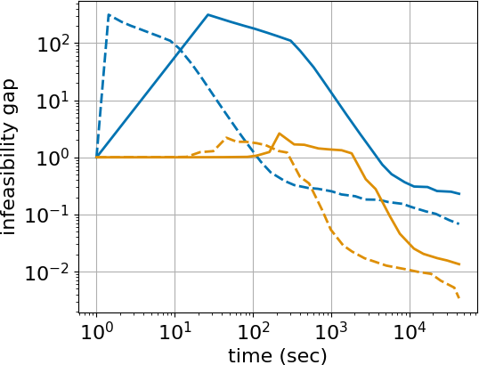
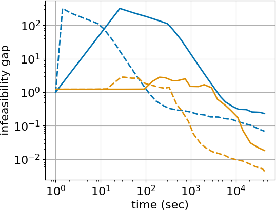
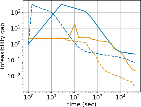
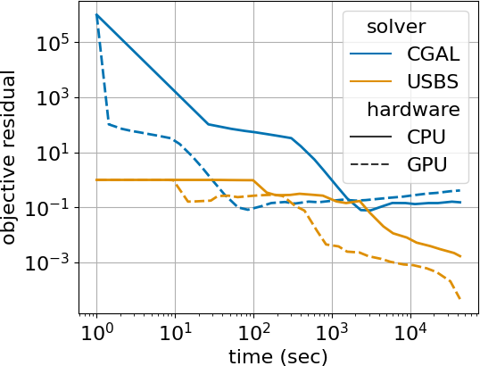
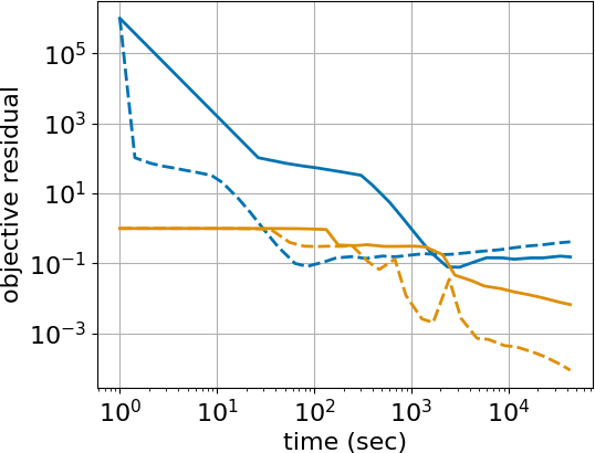
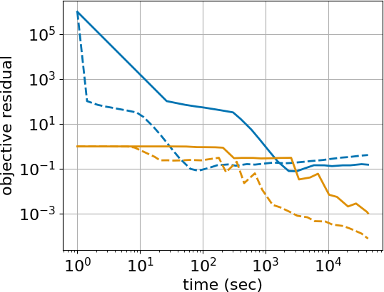
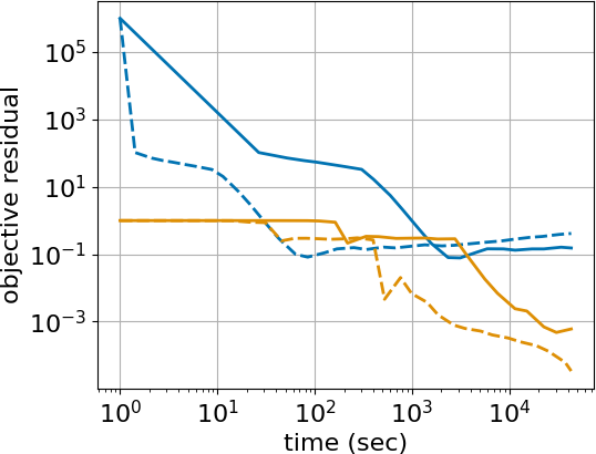
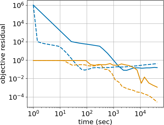
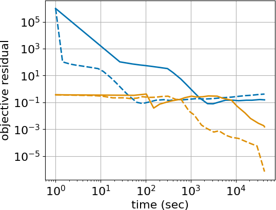
figs. 5 and 6 compare USBS’s infeasibility gap against time for different settings of and on the 144 instance from DIMACS10 on both CPU and GPU. figs. 7 and 8 compare USBS’s infeasibility gap against time for different settings of and on the 144 instance from DIMACS10 on both CPU and GPU. figs. 9 and 10 compare CGAL and USBS on CPU and GPU for different settings of and on the 144 instance from DIMACS10. We observe anywhere from 10-25x speedup on GPU as compared to CPU. We also observe that USBS performs best when .
F.2 QAP
Figure 11 and Figure 12 plot relative gap and best relative gap against time (in seconds) for three instances, respectively. Figure 11 shows that even for large instances the best relative gap is obtained within the first few minutes of the hour of optimization. In these instances, we can also observe that USBS not only obtains a better best relative gap, but also is able to leverage a warm-start solution to improve performance. Figure 13 shows the best relative gap obtained for ten data instances over one hour of optimization. It can be seen that warm-starting does not always yield a better best relative gap, but USBS is better able to leverage a warm-start solution than CGAL. These results show that warm-starting is a beneficial heuristic for finding a quality approximate solution to QAPs. The warm-starting technique used in these experiments is not the only possible warm-starting initialization strategy. For examples, one could generate several warm-start initializations for (21) by dropping other rows and columns of and besides the last row and column. Then, after creating n warm-start initializations, we could take the best upper bound obtained by optimizing (21) from each of those warm-start initializations.
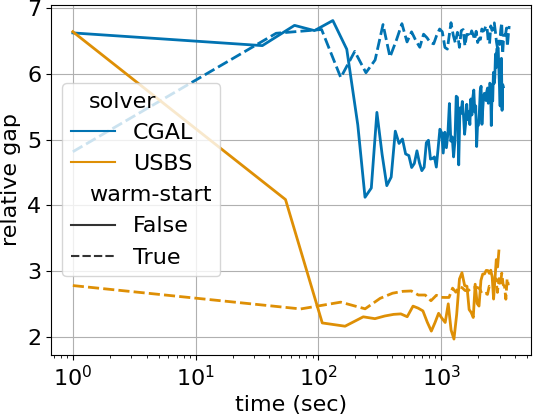
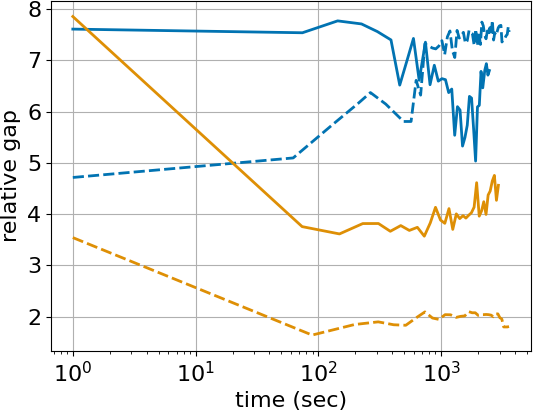
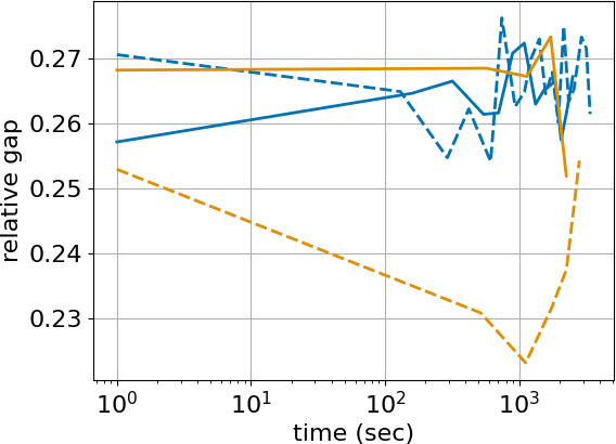
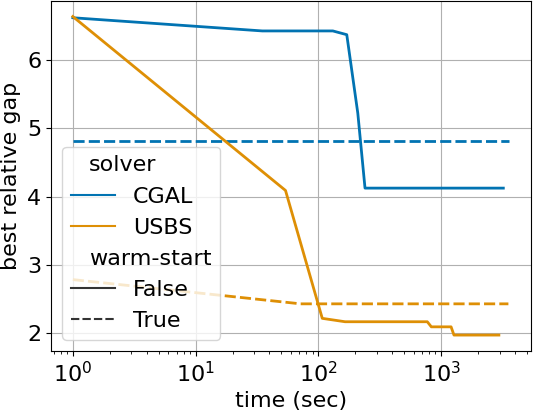
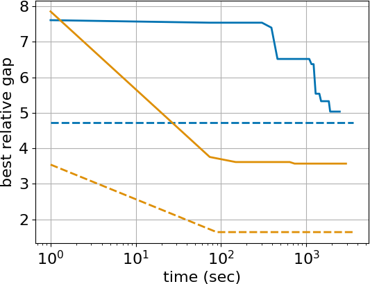
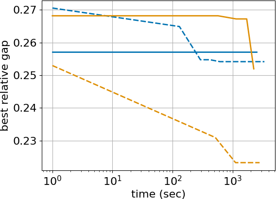
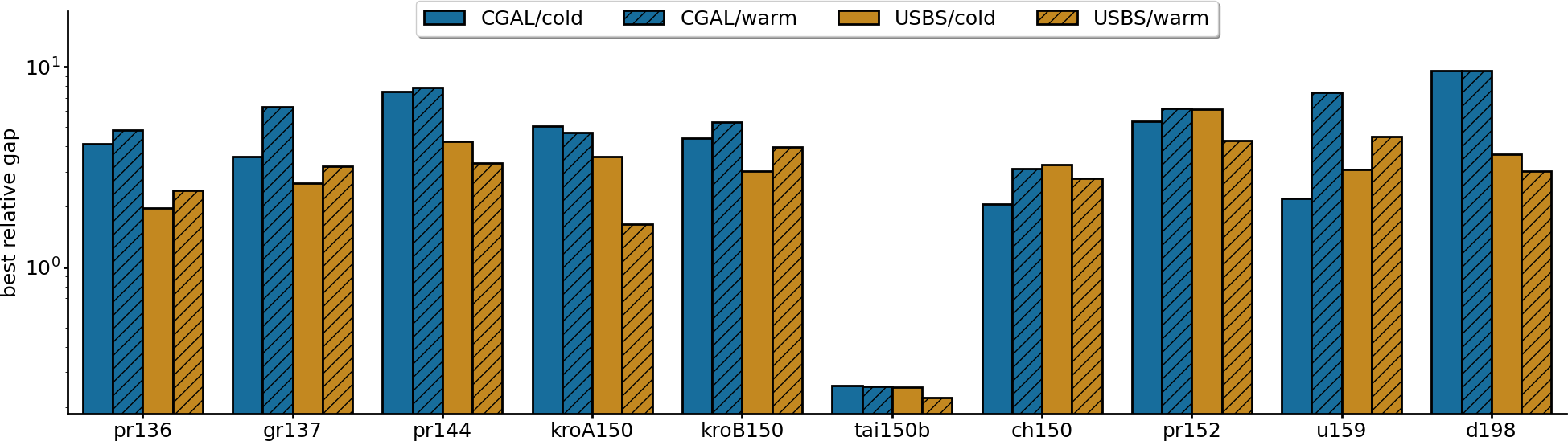
F.3 Interactive Entity Resolution with -constraints
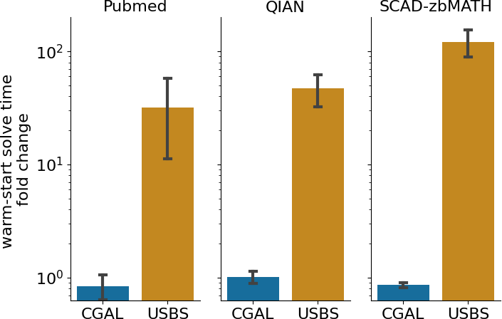
Figure 14 shows the average warm-start SDP solve time fold change. Warm-start fold change greater than one indicates a speedup in solve time while warm-start fold change less than one indicates a slowdown in solve time. We see that the warm-start fold change for CGAL is less than or equal to one, indicating a slowdown consistent with Figure 3. We see that on average warm-starting affords USBS a 20-100x speedup on average per -constraint . Note that this is much faster than the 2-3x we see in Figure 3. This is due to the fact that sometimes warm-starting does not help USBS, which makes intuitive sense if the warm-start initialization is far away from the solution set for the new SDP. We believe that with some further experimentation including additional pairwise learned similarities between mentions and -constraints or different warm-starting strategies we might be able to mitigate these situations. Regardless, in most cases, warm-starting provides a significant improvement in convergence time when using USBS. We also note that Figure 14 shows that warm-starting provides more of a benefit the larger the SDP we are trying to solve.