An effective image copy-move forgery detection using entropy image

Abstract

Image forensics has become increasingly important in our daily lives. As a fundamental type of forgeries, Copy-Move Forgery Detection (CMFD) has received significant attention in the academic community. Keypoint-based algorithms, particularly those based on SIFT, have achieved good results in CMFD. However, the most of keypoint detection algorithms often fail to generate sufficient matches when tampered patches are present in smooth areas. To tackle this problem, we introduce entropy images to determine the coordinates and scales of keypoints, resulting significantly increasing the number of keypoints. Furthermore, we develop an entropy level clustering algorithm to avoid increased matching complexity caused by non-ideal distribution of grayscale values in keypoints. Experimental results demonstrate that our algorithm achieves a good balance between performance and time efficiency.

Index Terms—  Image forensics, CMFD, SIFT, entropy level clustering

1 Introduction

With the advancement of multimedia technology, the quality of digital image forgeries has improved significantly. Simultaneously, the cost associated with such forgeries has decreased. Consequently, it has become increasingly challenging for people to trust the authenticity of images, unlike several decades ago. However, not all types of manipulations are concerned. In practical applications, people often focus on forgeries that cause semantic changes. In this scenario, copy-move and splicing have gained significant attention in the academic community. Currently, digital image forgery detection techniques can be classified into active and passive methods. Active techniques, such as digital watermarking and signatures, aim to detect tampering by verifying the integrity of pre-embedded prior information in the image. However, these techniques may affect the overall quality of the image. In contrast, passive techniques solely rely on the content information within the image itself and do not alter the original data, making them more widely applicable. Among the various manipulations, copy-move is particularly challenging due to its inherent similarity. Conventional, CMFD can be mainly divided into keypoint-based [1, 2, 3, 4, 5] and block-based [6, 7]. With the development of deep learning feature representation, deep-based [8, 9, 10, 11, 12] have gradually been applied in this field. The main differences between conventional algorithms and deep-based algorithms are as follows:

• Deep-based algorithms outperform conventional on low resolution images, but struggle with high resolution; Conventional algorithms can detect all image sizes, but take longer with high resolution images and rely on hand-crafted features for computer vision tasks.

• Deep-based algorithms still lack interpretability, while conventional algorithms are known for their good interpretability.

• Deep-based algorithms can be used to distinguish between source and target regions, while conventional algorithms struggle with this task.

Although deep-based algorithms have achieved great results, their application is limited when dealing with high resolution images. Therefore, we conducted research on the popular keypoint-based algorithms in CMFD. The keypoint-based is to generate uniformly distributed keypoints across the entire image. In existing works, detecting keypoints in gray images is the most commonly used approach [1, 3, 4, 5, 6, 7]. However, grayscale images primarily represent brightness and contrast information, making conventional keypoint detection algorithms less effective in regions with low texture. To address these issues, this paper proposes an effective CMFD algorithm, which includes as follows:

• We introduce entropy images to determine the coordinates and scales of keypoints. Since SIFT features represent the gradient information of the grayscale, we redefine the orientation and extraction feature in grayscale image, which makes our matching process more accuracy.

• We develop an entropy level clustering algorithm, which greatly address increased matching complexity caused by non-ideal grayscale distribution of keypoints.

The remainder of this paper is organized as follows. We detail our proposed method in section 2. Extensive experimental results are given in section 3, and section 4 draws the conclusion.

2 Proposed method

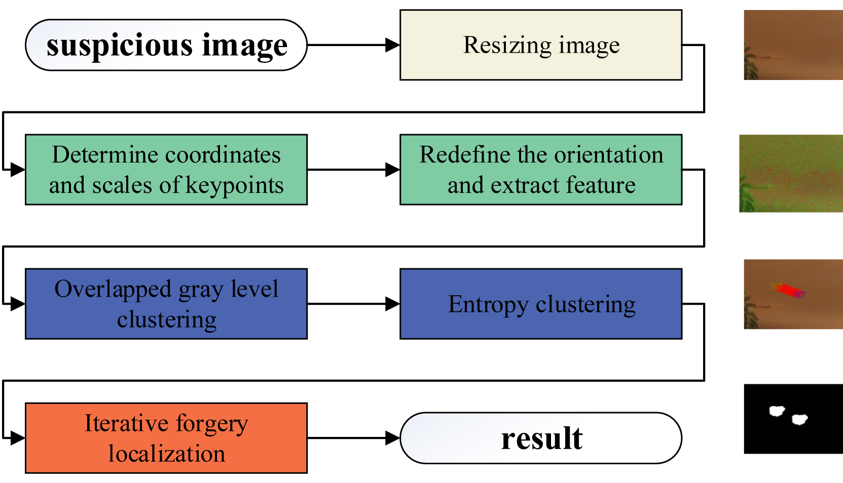
Fig. 1: Framework of the proposed algorithm.

As shown in Fig. 1, the framework of the proposed algorithm consists of three stage. For the third stage, we follow the method described in literature [1]. This post-processing was designed by fully exploiting the dominant orientation and scale information of each matched keypoint. Regarding the other stages, we will report them in the rest of this section.

2.1 Pre-processing

Compared to grayscale images, entropy images can effectively quantify the complexity of textures in a particular area, resulting in a denser distribution of keypoints obtained using entropy images. As shown in Fig. 2 (a), we select three different types of images from the GRIP dataset [6]. The first row represents high texture image, the second row represents an image with smooth and complex textures, and the third image represents a smooth image. The results of standard deviation filtering for the grayscale image and entropy image are represented by Fig. 2 (b) and (c) respectively. In order to provide readers with a better visual experience, we normalize the results to the range [0, 1] and display them using pseudocolored images. Obviously, Fig. 2 (c) exhibits a more suitable standard deviation distribution.

We observe that in the literature [1], the patches with the minimum variance are extracted to ensure that each patch generates 4 keypoints on GRIP [6]. This is necessary because RANSAC estimation requires a minimum of 4 correct matches. We highly appreciate this method as well. However, we observe that this method does not guarantee the presence of 4 correct matches within the copy-move patches after matching. To tackle this problem, We strives a strategy that aims to ensure the presence of 4 keypoints. Due to the commonly used block sizes for extracting invariant moment features range from $8\times 8$ to $32\times 32$, we choose the smallest size. Our objective is to generate a minimum of 4 keypoints within each $8\times 8$ region. We believe that this strategy will enhance the effectiveness of our CMFD.

Fig. 2 (d) and (e) represent the average density distribution of keypoints in grayscale images and entropy images, respectively. Obviously, the second and third types of images have a significant number of regions that do not meet our requirements. For detailed quantization results, please refer to Fig. 4 (b).

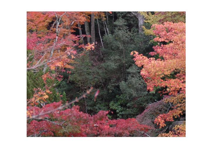
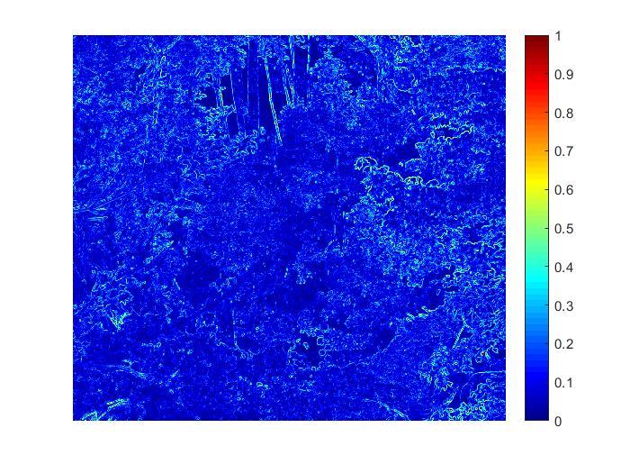
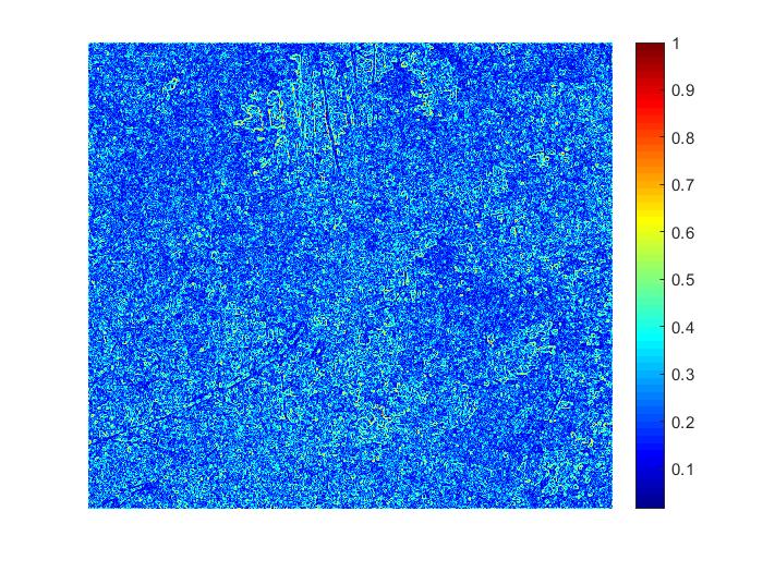
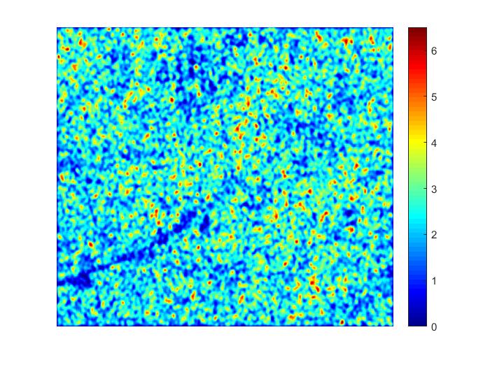
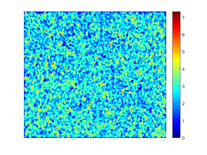
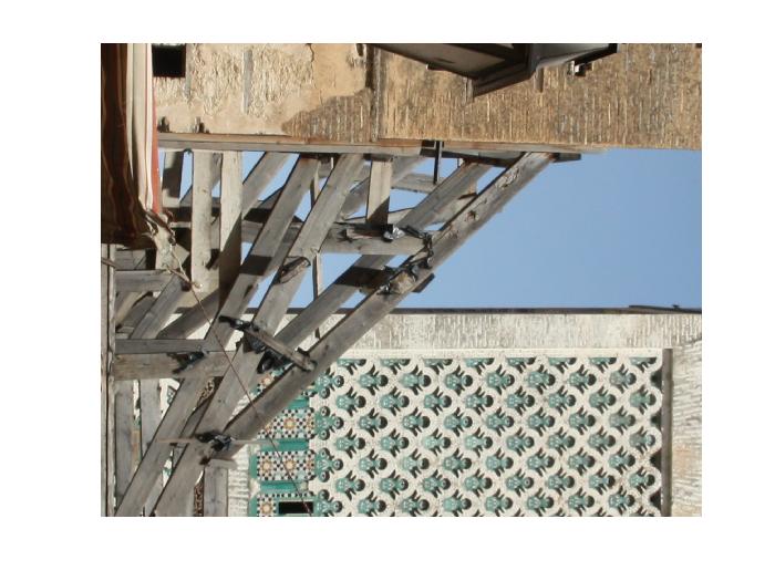
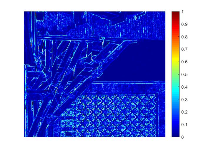
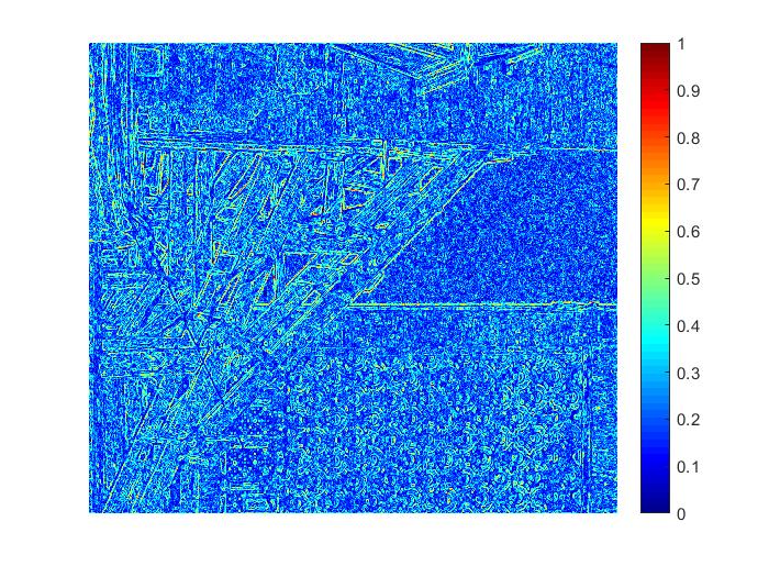
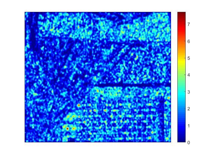
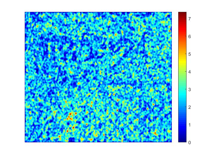
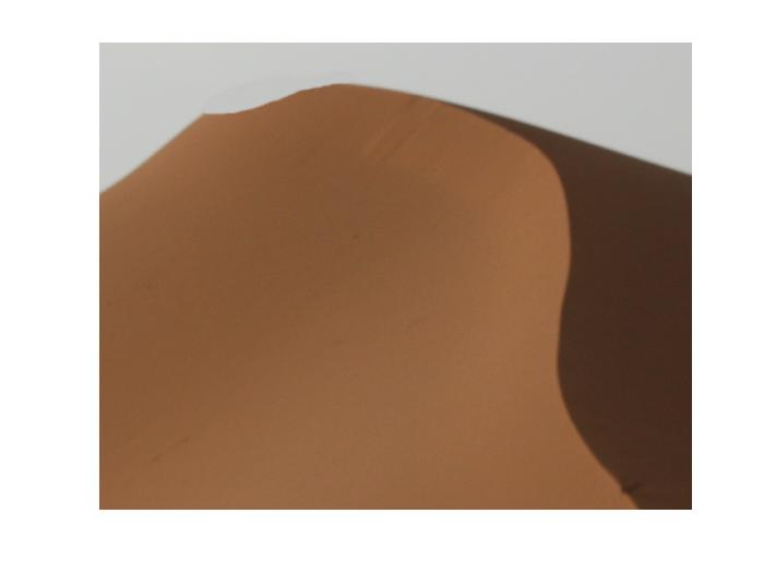
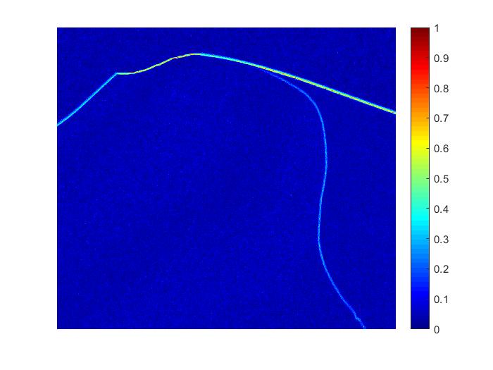
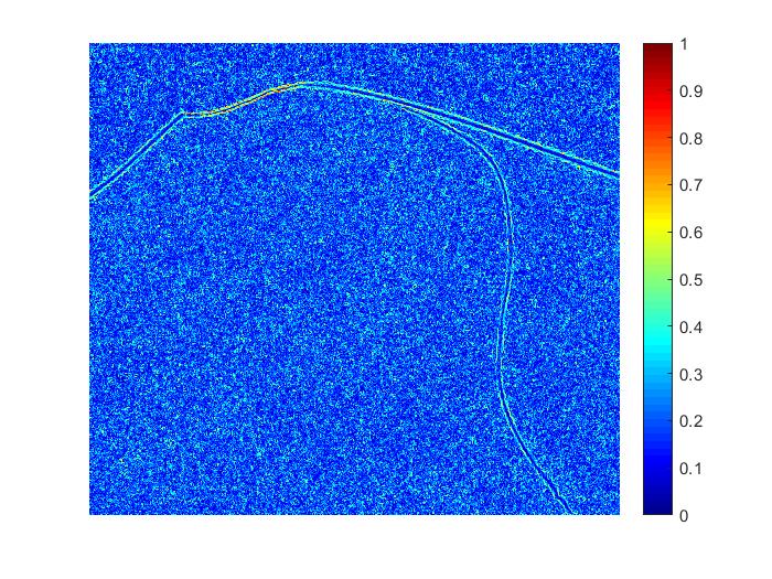
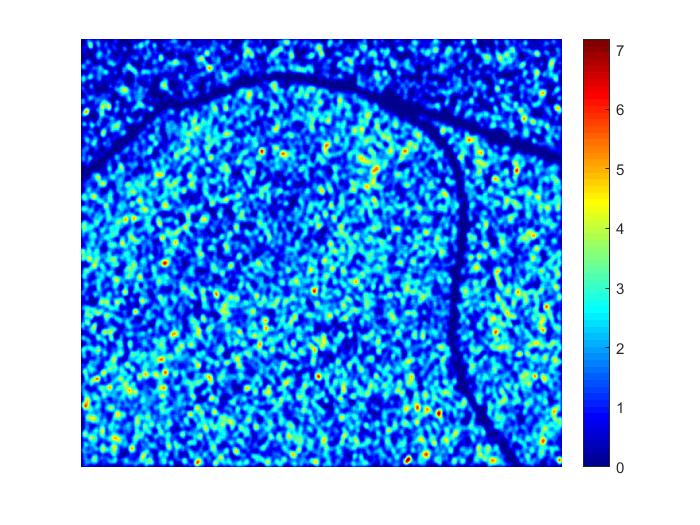
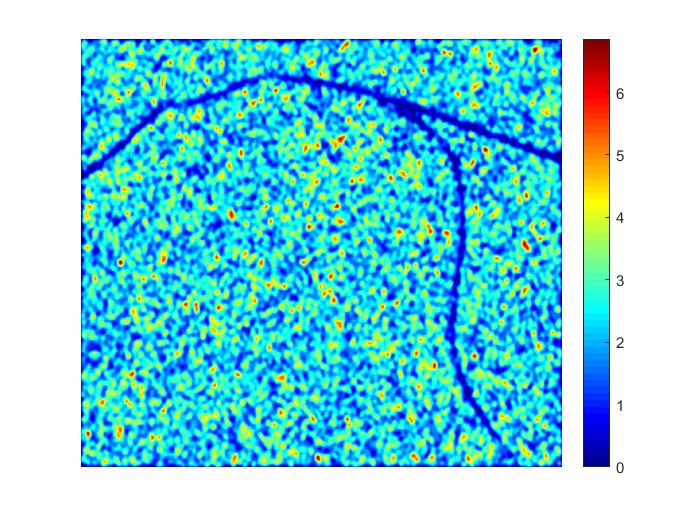
(a)	(b)	(c)	(d)	(e)

Fig. 2: Pre-processing results of different types of images. (a) RGB image; (b) the standard deviation of grayscale image; (c) the standard deviation of entropy image; (d) the average density distribution of keypoints in grayscale images; (e) the average density distribution of keypoints in entropy images.

Assuming the input grayscale image is denoted as $I$. We enlarge the size of $I$ by a scaling factor $s$ before detecting the SIFT keypoints. In this paper, the scaling factor $s$ defined as:

$$s=\left\{{\begin{array}[]{*{20}{l}}{2,\min(h,w)\leq 1024}\\ {{\rm{1,otherwise}}}\end{array}}\right.$$ (1)

Here, we define the upsampled image as $I_{gray}$ with width and height denoted as $w$ and $h$, respectively. For instance, if we have an image with dimensions $1024\times 728$ and we resize it with $s=2$, $I_{gray}$ will have dimensions of $2048\times 1456$.

Then, the entropy image $I_{E}(x,y)$ at position $(x,y)$ can be expressed as:

$${I_{E}}(x,y)=\sum\limits_{i=0}^{255}{{p_{i}}(x,y)\cdot{{\log}_{2}}[{p_{i}}(x,y)]}$$ (2)

Here, $p_{i}(x,y)$ represents the probability of the grayscale value being $i$ in a circular region with radius $R_{E}$ around $(x,y)$.

Subsequently, we apply the SIFT detector to extract keypoints $KP$ from $I_{E}(x,y)$. $KP$ can be defined as:

$$KP=\{x,y,\sigma\}$$ (3)

Here, $(x,y)$ are the coordinates in the image plane, $\sigma$ denotes scale information.

Finally, we will extract the dominant orientation $\theta$ of keypoints $KP$ and descriptor $DES$ from $I_{gray}$. $DES$ represents a 128-dimensional feature, and $KP$ can be represented as follows:

$$KP=\{x,y,\sigma,\theta\}$$ (4)

2.2 Hierarchical keypoint matching

2.2.1 Group matching via overlapped gray level clustering

Grayscale value can effectively reflect the basic information of an image, making it widely used in keypoint clustering algorithms. The major advantage of these methods is conducted in a much more efficient way without deleting original correct matches. This paper introduces a simple and effective overlapped gray level clustering method proposed in reference [1]. Formally, the group of overlapped gray level clustering can be expressed as:

$$\left\{{\begin{array}[]{*{20}{l}}{{C^{u}}=\{k{p_{i}}|{I_{gray}}(k{p_{i}})\in[a_{l}^{u},a_{h}^{u}),k{p_{i}}\in KP\}}\\ {a_{l}^{u}=(u-1)\cdot(ste{p_{1}}-ste{p_{2}})}\\ {a_{h}^{u}=\min(a_{l}^{u}+ste{p_{1}},255)}\end{array}}\right.$$ (5)

Here, $step_{1}$ represents the interval size, $step_{2}$ represents the overlapped size ($step_{1}>step_{2}$). The number of gray level groups is denoted as $N_{u}$, and it can be computed using the following equation:

$$N_{u}=\left\lceil{\frac{{255-step_{1}}}{{step_{1}-step_{2}}}}\right\rceil+1$$ (6)

2.2.2 Group matching via entropy level clustering

Although overlapped gray level clustering can be conducted in an effective way, its effectiveness will be significantly diminished when the grayscale values of keypoints are concentrated within a certain range. Fig. 3 (a) represents the grayscale distribution of the keypoints generated from a certain suspicious image. The grayscale values of keypoints are concentrated in the range of [150, 200], with approximately 70% of keypoints falling within this range according to our statistics. This will greatly reduce the efficiency of clustering matching. To tackle this problem, we propose the entropy level clustering algorithm. From Fig. 3 (b), it can be observed that even in cases where the grayscale distribution is not ideal, the entropy distribution still exhibits a favorable pattern. Therefore, we can make a reasonable partition on the two-dimensional plane of grayscale and entropy values to address the problem mentioned above. A typical example is illustrated in Fig. 3 (c).

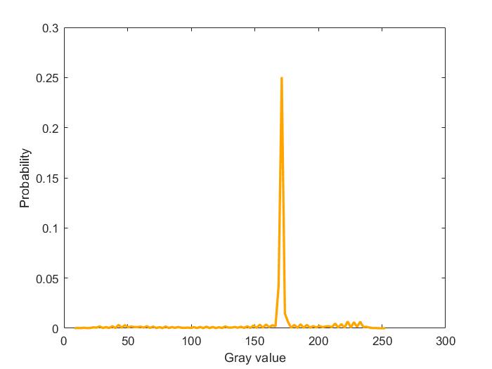
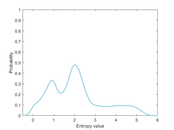
(a)	(b)
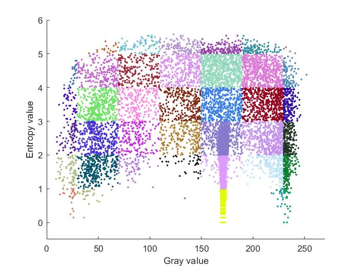
(c)

Fig. 3: An example of hierarchical feature point clustering. (a) the gray value distribution of the keypoints; (b) the entropy value distribution of the keypoints; (c) hierarchical keypoint clustering.

The entropy level clustering algorithm can be expressed as follows:

$${C^{u,v}}=\{k{p_{i}}|{I_{E}}(k{p_{i}})\in[v-1,v],k{p_{i}}\in{C^{u}}\}$$ (7)

Due to the fact that entropy value is controlled by $R_{E}$, it is evident that all entropy values are distributed within the range of [0, 7]. Hence, $v=1,2,\cdots,7$.

After implementing hierarchical keypoint clustering, we will proceed with grouping and matching $C^{u,v}$, ensuring that the matching process satisfies:

$${d_{i}}<T\cdot{d_{i+1}},i=2,\cdots{n_{u,v}}$$ (8)

Here, $n_{u,v}$ represents the number of keypoints within $C^{u,v}$’s group, and $d$ represents the ascending distance between a certain feature and all features within $C^{u,v}$. For the post-processing stage, we adhere to the iterative forgery localization algorithm used in reference [1].

3 Experiments

In this section, we evaluate our proposed method via a series of simulation experiments. All the experiments are done using MATLAB R2018a under Microsoft Windows. The PC used for testing has 2.30 GHz CPU and 16 GB RAM.

3.1 Datasets

This paper validates the proposed algorithm using two public datasets, with details as follows:

• GRIP: This dataset [6] contains 80 tampered images and 80 original images, all of which are in the size of $1024\times 768$ pixels. Some of the images in this dataset include smooth regions, allowing for effective evaluation of the scheme’s performance in such regions.

• CMH: This dataset [2] consists of 108 tampered images with resolutions ranging from $845\times 634$ to $3888\times 2592$ pixels.

3.2 Evaluation metrics

Generally, the evaluation of copy-move forgery detection techniques can be performed at two levels: image level and pixel level. At the image level, the objective is to accurately determine whether an image is tampered with or original. At the pixel level, a more stricter criterion is applied, emphasizing the localization of tampered regions within the image. Usually, datasets commonly employ three evaluation metrics, which are defined as follows:

$$TPR=\frac{{TP}}{{TP+FN}}$$ (9)

$$FPR=\frac{{FP}}{{TN+FP}}$$ (10)

$$F=\frac{{2TP}}{{2TP+FP+FN}}$$ (11)

In the equation mentioned above, TP represents the number of correctly detected tampered images or pixels, TN represents the number of correctly detected original images or pixels, FN represents the number of incorrectly detected tampered images or pixels, and FP represents the number of incorrectly detected original images or pixels.

3.3 Analysis of parameters

In this section, we mainly analyze the parameters of $s$ and $R_{E}$ in Section 2.1.

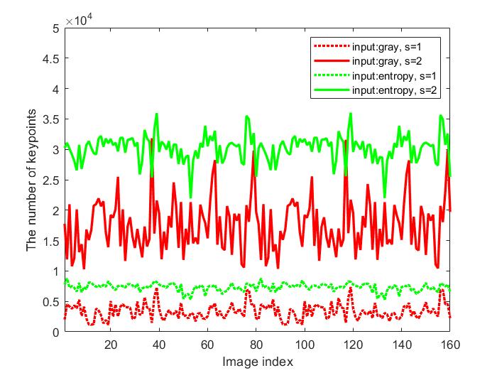
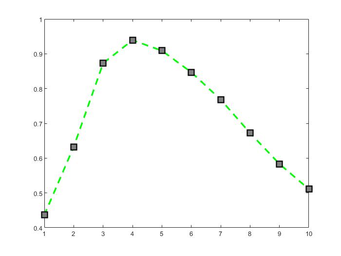
(a)	(b)

Fig. 4: The analysis of parameters. (a) the number of keypoints generated for different inputs and $s$; (b) the rate of pixels with more than 4 keypoints within an $8\times 8$ block under different $R_{E}$.

As shown in Fig. 4 (a), we conduct tests using the GRIP dataset, and the results indicate that regardless of grayscale or entropy images, increasing the upsampling once will approximately triple the number of detected keypoints. Furthermore, by keeping $s$ unchanged, we can clearly observe that the entropy image yields approximately 1.5 times more keypoints compared to the grayscale image. This demonstrates that entropy images are more suitable for CMFD than grayscale images.

As shown in Fig. 4 (b), we calculate the rate of pixels with more than 4 keypoints within an $8\times 8$ block under different $R_{E}$. In addition, 58.84% for grayscale images is obtained under the same conditions. Clearly, entropy images yields better results compared to grayscale images when $R_{E}$ is within the range [2, 8], and the highest ratio that meets our requirements occurs at $R_{E}=4$. Therefore, this paper adopts $R_{E}=4$.

3.4 Detection results on different datasets

In the early phase of our algorithm design, we prioritized testing on the CMH dataset due to limited previous research on this dataset. However, we note that CMH dataset contains forgery images only. In this work, we adopt a combined dataset named CMH+GRIPori, consisting of all the 108 forgeries from CMH, and the 80 original images from GRIP dataset. Some results of the testing are shown in Fig. 5.

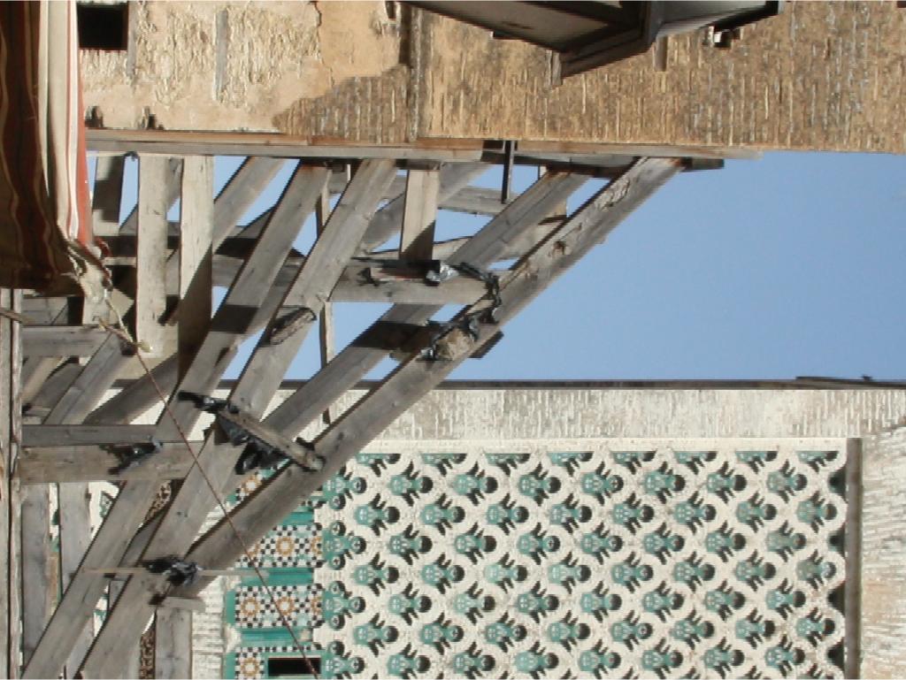
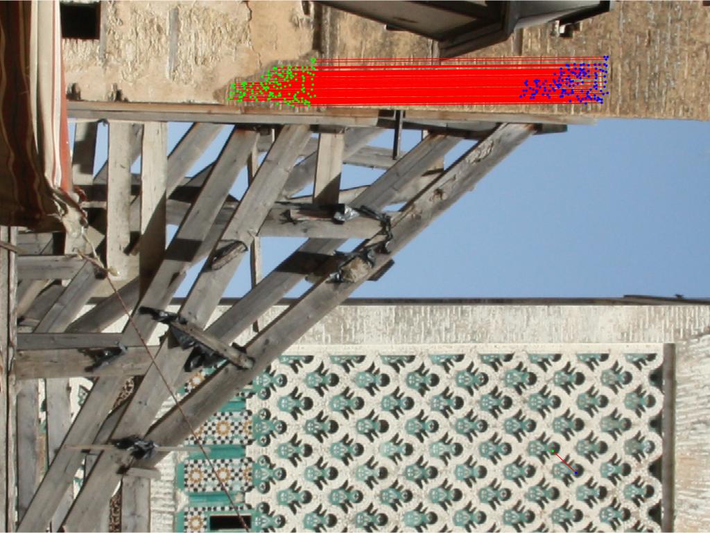
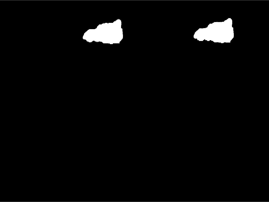
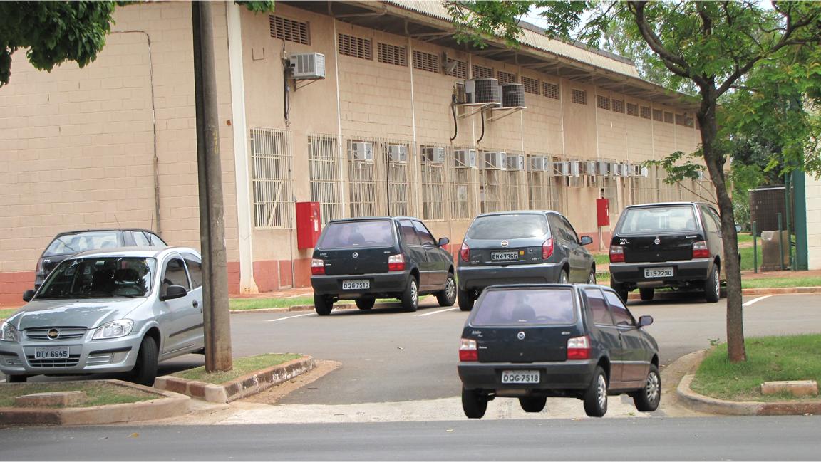
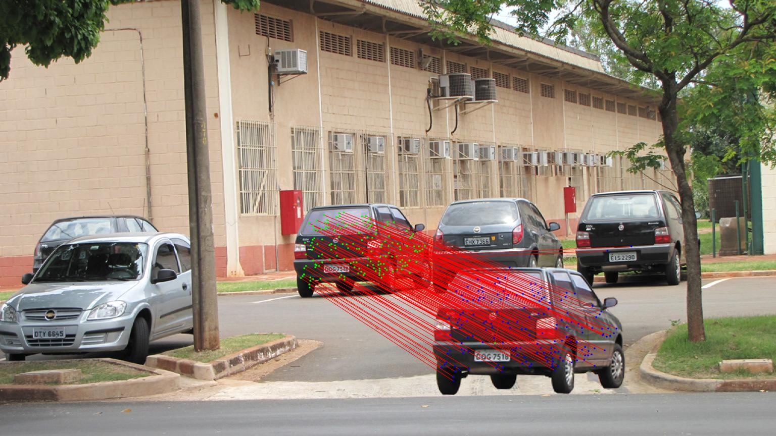
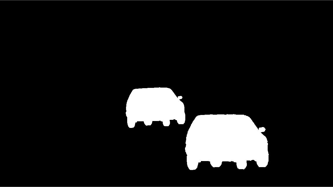
(a)	(b)	(c)	(d)

Fig. 5: Some results of the testing. (a) forgery images; (b) matching; (c) binary result; (d) ground-true.

Table 1 lists the results on CMH+GRIPori obtained by different CMFD, including keypoint-based [1, 2, 3], block-based [6] and proposed method. To provide more detailed test results, we use TPR and FPR to represent image level TPR and FPR metrics, while F-i and F-p represent image level and pixel level F metrics, respectively. Obviously, our proposed method achieve the best results on the CMH+GRIPori dataset.

Table 2 lists the results on GRIP. we can observe that our proposed method has achieved promising results on this dataset as well. However, our method has a disadvantage in terms of time complexity, but this is not due to the design of the matching process. According to the analysis in section 3.3, we find that our method obtains approximately 1.5 times the number of keypoints compared to the generated grayscale images. Typically, the time complexity is directly proportional to the square of the number of keypoints. Based on this estimation, our matching efficiency is approximately 29% faster than the state-of-the-art method mentioned in reference [3] when tested on the GRIP dataset.

Table 1: the results on CMH+GRIPori

Methods	TPR	FPR	F-i	F-p	time
[1]	96.3	0	98.11	90.61	11.2s
[2]	95.37	38.75	85.12	64.09	18.1s
[3]	99.07	0	99.53	91.72	43.3s
[6]	92.59	8.75	93.02	88.10	13.1s
proposed	99.07	0	99.53	92.47	19.9s

Table 2: the results on GRIP

Methods	TPR	FPR	F-i	F-p	time
[1]	100	0	100	94.66	13.9s
[2]	100	38.75	83.77	66.62	11.7s
[3]	100	0	100	98.57	12.9s
[6]	98.75	8.75	95.18	92.99	14.8s
proposed	100	0	100	95.47	20.6s

4 Conclusion

In this paper, we propose a novel framework for CMFD using entropy image. Firstly, we introduce entropy images to determine the coordinates and scales space of keypoints. Considering SIFT features represent the gradient information of the grayscale, we redefine the orientation and extraction feature in grayscale image, which makes our matching process more accuracy. Then, an entropy level clustering is developed to avoid increased matching complexity caused by non-ideal distribution of grayscale values in keypoints. Experimental results demonstrate that our algorithm achieves a good balance between performance and time efficiency.

References

- [1] Yuanman Li and Jiantao Zhou, “Fast and effective image copy-move forgery detection via hierarchical feature point matching,” IEEE Transactions on Information Forensics and Security, vol. 14, no. 5, pp. 1307–1322, 2018.
- [2] Ewerton Silva, Tiago Carvalho, Anselmo Ferreira, and Anderson Rocha, “Going deeper into copy-move forgery detection: Exploring image telltales via multi-scale analysis and voting processes,” Journal of Visual Communication and Image Representation, vol. 29, pp. 16–32, 2015.
- [3] Pan-pan Niu, C Wang, W Chen, Hongying Yang, and Xiangyang Wang, “Fast and effective keypoint-based image copy-move forgery detection using complex-valued moment invariants,” Journal of Visual Communication and Image Representation, vol. 77, pp. 103068, 2021.
- [4] Patrick Niyishaka and Chakravarthy Bhagvati, “Copy-move forgery detection using image blobs and brisk feature,” Multimedia Tools and Applications, vol. 79, no. 35-36, pp. 26045–26059, 2020.
- [5] Qiyue Lyu, Junwei Luo, Ke Liu, Xiaolin Yin, Jiarui Liu, and Wei Lu, “Copy move forgery detection based on double matching,” Journal of Visual Communication and Image Representation, vol. 76, pp. 103057, 2021.
- [6] Davide Cozzolino, Giovanni Poggi, and Luisa Verdoliva, “Efficient dense-field copy–move forgery detection,” IEEE Transactions on Information Forensics and Security, vol. 10, no. 11, pp. 2284–2297, 2015.
- [7] Seung-Jin Ryu, Matthias Kirchner, Min-Jeong Lee, and Heung-Kyu Lee, “Rotation invariant localization of duplicated image regions based on zernike moments,” IEEE Transactions on Information Forensics and Security, vol. 8, no. 8, pp. 1355–1370, 2013.
- [8] Yingjie He, Yuanman Li, Changsheng Chen, and Xia Li, “Image copy-move forgery detection via deep cross-scale patchmatch,” in 2023 IEEE International Conference on Multimedia and Expo (ICME). IEEE, 2023, pp. 2327–2332.
- [9] Yue Wu, Wael Abd-Almageed, and Prem Natarajan, “Busternet: Detecting copy-move image forgery with source/target localization,” in Proceedings of the European conference on computer vision (ECCV), 2018, pp. 168–184.
- [10] Beijing Chen, Weijin Tan, Gouenou Coatrieux, Yuhui Zheng, and Yun-Qing Shi, “A serial image copy-move forgery localization scheme with source/target distinguishment,” IEEE Transactions on Multimedia, vol. 23, pp. 3506–3517, 2020.
- [11] Ashraful Islam, Chengjiang Long, Arslan Basharat, and Anthony Hoogs, “Doa-gan: Dual-order attentive generative adversarial network for image copy-move forgery detection and localization,” in Proceedings of the IEEE/CVF conference on computer vision and pattern recognition, 2020, pp. 4676–4685.
- [12] Jun-Liu Zhong, Ji-Xiang Yang, Yan-Fen Gan, Lian Huang, and Hua Zeng, “Coarse-to-fine spatial-channel-boundary attention network for image copy-move forgery detection,” Soft Computing, vol. 26, no. 21, pp. 11461–11478, 2022.