Hyperdimensional Computing Provides a Programming Paradigm for Oscillatory Systems

Abstract

The increased difficulty in continuing to develop digital electronic logic has led to a renewal of interest in alternative approaches. In this work, we provide a model based on hyperdimensional computing for integrating oscillatory devices into larger computational systems. The expressiveness and compositionality of the underlying computing model allows oscillatory systems to implement both common tasks and novel functions, providing a computational role for many classes of emerging hardware devices. Furthermore, we detail the computational primitives of this system, prove how they can be executed via oscillatory systems, quantify the performance of these operations, and apply them to execute a graph compression task.

I Introduction

The rate of progress in computing based on digital electronic logic has slowed, creating a challenge for an information economy accustomed to a rapid pace of hardware improvement [1]. This challenge has motivated numerous responses, including increased hardware specialization, exploration of alternative representations of information, and the development of novel hardware devices [2, 3, 4]. Among these approaches, the development of novel hardware devices offers unique opportunities to utilize and manipulate alternative physical representations of information. These include physical properties such as optical polarization, electronic spin, and others [4]. Utilizing these alternate physical properties can yield systems with entirely different scaling properties than traditional digital electronics. For instance, photonic systems demonstrate the ability to increase throughput via wavelength-division multiplexing and carry out multiply-accumulate operations with no active power [5].

However, it is a major challenge to integrate even a promising device into a larger system which can carry out useful tasks. The history of computing contains a multitude of alternative visions which were unsuccessful due to their lack of scalability or compatibility with mainstream applications [6]. Compatibility with a broader model of computing provides one reassurance that a novel device can meet the end goal of being integrated within a system that provides utility to a significant user base.

We propose that an established mode of computing, termed ‘hyperdimensional’ (HD) or ‘vector-symbolic’ computing, provides a rich model for information processing requiring operations that can be expressed by many emerging devices. Specifically, we investigate one HD computing system which represents information via phase angles. This provides a specific domain on which an emerging device (or circuit of devices) can express values. Linking ensembles of these elements provides a method to scale into a full computational system. Furthermore, work has already established that this mode of computation can efficiently and composably express popular applications such as neural networks, finite state machines, graph queries, and more [7].

In this work, we detail the computational primitives used by this computing system and how they can operate both by traditional floating-point implementations and novel oscillator-based circuits. We quantify the differences in performance between these implementations and demonstrate a graph compression task. Lastly, we make a scalable and open-source demonstration of these computations available.

II Representation in Computing

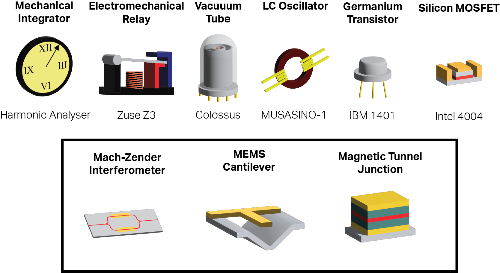
Figure 1: Illustration of artificial devices employed to represent abstract values. Many devices (top text) have been employed to construct practical computing devices (bottom label), but other emerging devices (inner box) are still being investigated for this use.

The representation of information within a computer system greatly influences its performance characteristics. While any two Turing-complete computers may be theoretically have the same capabilities, in reality one may provide much greater advantages on certain tasks given the presence of specialized hardware [8, 9]. Much of this specialized hardware focuses on manipulating the fields of rational and real numbers, often represented (or approximated) by digital electronic elements (Fig. 1). Analog representations of these fields are also being investigated for potential advantages in power efficiency and storage density, though this requires a trade-off from deterministic to stochastic computation [10, 11].

III Phase Vectors

HD computing identifies novel computing methods which employ phenomena encountered in high-dimensional spaces [17], [18]. The fundamental units of information (symbols) in these systems consist not of a single value, but rather a long vector of values – generally, at least hundreds of values. Based on the HD system being used (several exist), each of these values may be binary, real-valued, or complex [19]. In this work, we employ the Fourier Holographic Reduced Representation (FHRR) system, in which each a symbol is defined by vector of angular values, or equivalently, a vector of complex values on the unit circle (1) [20], [21].

$$\bm{\phi}\in FHRR=[\phi_{1},\phi_{2},\ldots,\phi_{n}]=[e^{i\phi_{1}},e^{i\phi_{2}},\ldots,e^{i\phi_{n}}]$$ (1)

III-A Similarity

As a distance can be defined between two real numbers on the ‘number line,’ so can a distance be defined between two HD symbols. This distance can be found by first computing the “similarity” between two symbols [7]. Computing this similarity requires finding the phase difference between each element of the two symbols, measuring its cosine distance, and taking the average value of these distances (2). Vectors of phases with n elements are represented by $\bm{\phi}_{0}$ and $\bm{\phi}_{1}$ .

$$similarity(\bm{\phi}_{0},\bm{\phi}_{1})=\frac{1}{n}\sum_{k=1}^{n}cos(\bm{\phi}_{0,k},\bm{\phi}_{1,k})$$ (2)

The distance between two symbols can then be measured by subtracting the similarity value from 1 – the maximum similarity (closeness) between two symbols (3).

$$distance(\bm{\phi}_{0},\bm{\phi}_{1})=1-similarity(\bm{\phi}_{0},\bm{\phi}_{1})$$ (3)

Two symbols which are identical therefore have a similarity of 1 and distance of 0. In the FHRR, this implies that each pair of angles between the two symbols is exactly in-phase. Alternatively, when on average the angles are orthogonal, the similarity between the symbols will be 0 and their distance is 1. Symbols which contain angles exactly opposing one another have a similarity of -1 and distance of 2 (Fig. 2).

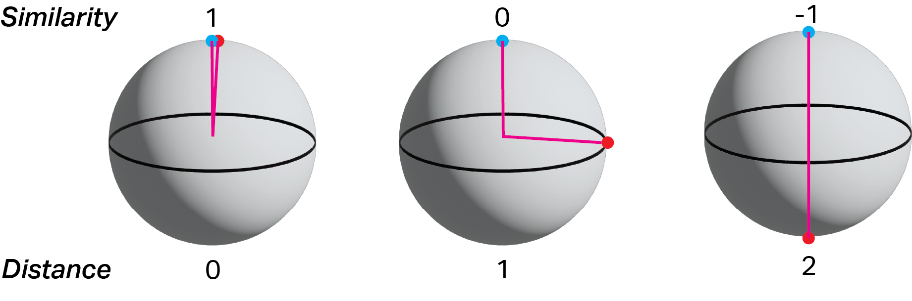
Figure 2: Illustration of similarity between HD symbols. Each FHRR symbol can be embedded on the surface of a hypersphere. Coincident points are similar (in-phase), orthogonal points are dissimilar (out-of-phase), and points on opposite ends of the hypersphere are opposing (antiphase). The central limit theorem implies that as the number of elements in a symbol increase, the likelihood that two random symbols are dissimilar tends towards 1.

III-B Bundling

‘Bundling’ is an operation which loosely corresponds to addition, where multiple symbols are reduced into a single output which is maximally similar to its inputs (Fig. 3). Creating a symbol which is maximally similar to a set of inputs requires that the cosine distance between phases in the inputs and the output phase be minimized. This is done for m input symbols by converting each phase to an explicitly complex value and taking the argument of their sum (4).

$$\bm{\phi}^{\prime}=bundle(\bm{\phi}_{0},\bm{\phi}_{1},\ldots,\bm{\phi}_{m})=arg(\sum_{k=1}^{m}e^{i\bm{\phi}_{k}})$$ (4)

Bundling can be used as a form of lossy compression, for instance representing a set of input symbols (“apple, banana, grape”) as a single output (“fruits”). The constructed output is maximally similar to each of the input symbols. In general, symbols can be bundled until the similarity of the output to each of the inputs degrades to the level seen between random symbols. If inputs already retain a degree of similarity to one another, many may be effectively bundled together. Dissimilar inputs may also be bundled together to produce a similar output, but fewer can be included before the level of similarity degrades to the chance level [7].

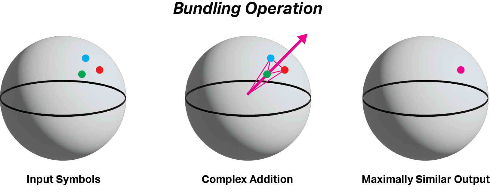
Figure 3: Illustration of the FHRR bundling operation. A set of points is combined through addition in the complex domain. The argument of this vector is taken to find a point on the surface of a hypersphere which is maximally similar to the set of inputs.

The inverse operation of bundling can also be carried out by scaling the output vector and removing the inputs which were added to reach it. However, this requires retrieving the other vectors which were combined to produce the output (5).

$$\begin{split}\bm{\phi}_{0}=unbundle(\bm{\phi}^{\prime},(\bm{\phi}_{1},\ldots,\bm{\phi}_{m}))\\ =arg[m\cdot e^{i\bm{\phi}^{\prime}}+\sum_{k=1}^{m}(-1+0i)\cdot e^{\bm{\phi}_{k}}]\end{split}$$ (5)

III-C Binding

‘Binding’ is an operation which corresponds to multiplication, in which a set of inputs can be displaced by another singular vector (Fig. 4). Carrying out the binding operation is simple in the phase domain; one phase value is offset by another – “adding” the two angles together (6). The resulting outputs can be dissimilar to the inputs, but the relationship of similarities between inputs is preserved.

$$\bm{\phi}^{\prime\prime}=bind(\bm{\phi}_{0},\bm{\phi}_{1})=\bm{\phi}_{0}+\bm{\phi}_{1}$$ (6)

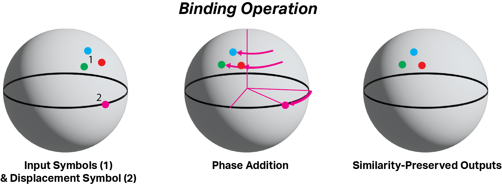
Figure 4: Illustration of the FHRR binding operation. A set of inputs (1) is displaced by a second symbol (2). The angular values of this symbol are added to the set of inputs in the phase domain, shifting each equally. This “orbits” the points around the surface of the hypersphere, maintaining each symbol’s similarity to one another but making them dissimilar to their original values.

Binding can also be inverted through subtraction (7)

$$\bm{\phi}_{0}=unbind(\bm{\phi}^{\prime\prime},\bm{\phi}_{1})=\bm{\phi}^{\prime\prime}-\bm{\phi}_{1}$$ (7)

Binding can be employed to many ends, for instance to construct hierarchical relationships in HD spaces. For instance, to represent a family member, a person’s name can be bound with their role – for instance, “Alice” with “Sister.” Multiple relatives can then be combined through bundling to produce a compressed family tree.

III-D Summary

By applying the atomic operations of bundling and binding, a large variety of useful applications can be expressed, including finite state machines, data structures, string processing, and more [22]. By supplementing these operations with standard linear algebra, HD computing can also be used to implement neural networks [23, 24, 25]. Beyond conventional computing, HD computing also offers the ability to compute multiple queries in superposition and efficiently encode and compute with sparse information [26, 27, 28]. Furthermore, in this work we firmly establish the connection between the atomic FHRR operations and their ability to be executed on oscillator-based systems.

IV Oscillators

Numerous natural systems exhibit oscillatory behavior: fireflies, the human heart, and pendulum clocks are all oscillators. Utilizing power from an internal source, they maintain regular, self-sustaining periodic activity which follows a regular ‘limit cycle’ around an attractor in their phase space [29]. In a pendulum clock, the motion of the pendulum continuously converts the oscillator’s energy from potential to kinetic and back again. The interchange between these two domains can be expressed as a system of linear differential equations (8), where $x$ and $y$ represent variables such as the position and angular velocity of a pendulum, $b$ represents the ‘damping’ or loss of the oscillator, and $\omega$ represents its angular frequency.

$$\frac{dx}{dt}=-\omega y+bx,\frac{dy}{dt}=\omega x+by$$ (8)

These two separate variables can be transformed into a single, complex-valued argument or ‘state’ which evolves through time given a single equation (9), where $Z$ is the complex state and $i$ is the imaginary unit [30].

$$\frac{dZ}{dt}=(b+i\omega)Z$$ (9)

Biological neurons can also be viewed as fundamentally oscillatory devices, as they exhibit frequency resonances and other complex behaviors. For this reason, Equation 9 is used as the basis for the resonate-and-fire neuron model, where the real part of the state represents the membrane current of a neuron and the imaginary part represents its membrane potential [30].

When the damping value $b$ of (9) is small compared to the angular frequency $\omega$, the state of the system can be approximated over a limited period of time by Euler’s formula, (10) which traces a circle around the origin of the complex plane. The value $\phi$ represents the ‘starting phase’ of the oscillator which arises as an integration constant.

$$Z=e^{i(\omega t+\phi)}$$ (10)

The state of this oscillator at an instant in time can then be described as a single value – its angular position in the complex plane, known as its instantaneous phase. This instantaneous phase changes continuously with time as the oscillator’s state evolves.

The evolution of this system in the complex plane and ability to maintain and manipulate phase values suggests that it can provide a basis for HD computing with the FHRR system. In the following sections, we prove that this intuition is correct.

V HD Operations via Oscillators

V-A Representing Phase

To utilize oscillatory elements to represent and compute with the phase values used in the FHRR HD system, it is necessary to encode these values in a way which remains invariant with time. To do this, two oscillators with the same fundamental frequency can be used. Stable phase values can then be encoded not in each oscillator’s instantaneous phase, but in their relative phase, which remains constant with time (11, Supplementary Proof 1). The time-invariance of the relative phase of frequency-locked oscillators endows these systems with the ability to compute using the FHRR computing system. In other words, frequency-locked oscillators will maintain the differences between their starting phases through time.

$$\frac{\partial}{\partial t}\angle(Z_{1}(\phi_{1})-Z_{0}(\phi_{0}))\propto\frac{\partial}{\partial t}\|Z_{1}-Z_{0}\|=0$$ (11)

We now derive the methods via which systems of oscillators storing relative phase values can carry out the computations necessary for the FHRR HD computing system: similarity, bundling, and binding.

V-B Similarity

These phases can be encoded into complex state of oscillators by employing them as the starting phase of each oscillator (10). The value of interest (the relative phase between each oscillator) will remain constant through time. Recalculating the explicit phase and computing the cosine difference between these phase angles appears necessary to compute similarity. However, this operation can be achieved more simply by superimposing the complex state of pairs of oscillators (Supplementary Proof 2), where $\bm{Z}_{0}$ and $\bm{Z}_{1}$ represent vectors of complex oscillator states with $n$ elements each. This interference between the oscillators is proportional to the cosine similarity between their phase values (12)(Fig. 5).

$$sim.(\bm{Z}_{0},\bm{Z}_{1})=\frac{1}{n}\sum^{n}_{i=1}cos[2\cdot arccos(\frac{\|\bm{Z}_{0,i}+\bm{Z}_{1,i}\|}{2})]$$ (12)

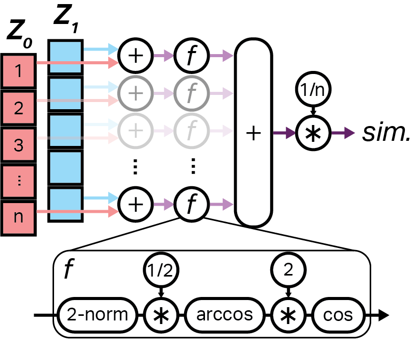
Figure 5: An illustration of the similarity operation executing on two HD symbols encoded into oscillators. The complex values from two paired oscillators are superimposed and transformed. This operation is carried out for each pair of values between two HD symbols and reduced through averaging.

V-C Bundling

Bundling consists of a normalized superposition carried out in the complex plane. As oscillators already encode phases in the complex domain, taking a normalized sum of their m complex states carries out the bundling operation (13)(Fig. 6).

$$bundle(\bm{Z}_{0},\bm{Z}_{1},\ldots,\bm{Z}_{m})=\frac{1}{m}\sum^{m}_{k=1}\bm{Z}_{k}$$ (13)

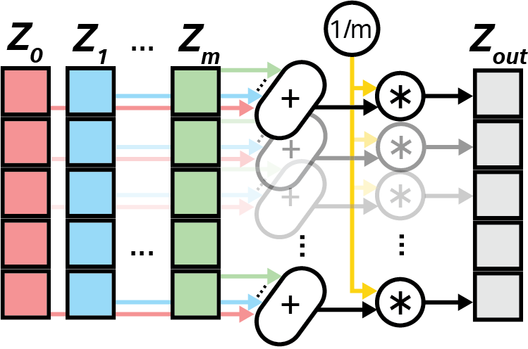
Figure 6: An illustration of the bundling operation executing on an arbitrary number of HD symbols encoded into oscillators. The complex values from each oscillator in the same row are reduced through summation and normalized by the number of HD symbols to produce the output.

V-D Binding

Carrying out bundling in the complex domain via the interaction of oscillators is more involved than the previous two operations, where superposition sufficed to compute the necessary values. In the case of binding, multiplication of complex values becomes necessary as well as the inclusion of a reference state (Supplemental Proof 3). This reference defines what complex state currently represents the angle 0, allowing the displacement vector for the input to be correctly calculated, rotating the input to a new complex value (14(Fig. 7).

$$bundle(\bm{Z}_{0},\bm{Z}_{1},\ldots,\bm{Z}_{m})=\frac{1}{m}\sum^{m}_{k=1}\bm{Z}_{k}$$ (14)

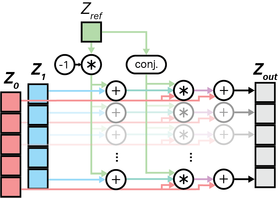
Figure 7: An illustration of the binding operation executing on two HD symbols encoded into oscillators. To decode the absolute phase values stored in these oscillators, a reference oscillator representing the angle 0 is included. The negation and complex conjugate of this reference oscillator are used to (1) decode the absolute phase of the second input and (2) maintain a frequency-matched output oscillation.

V-E Inverse Operations

As bundling takes place in the complex domain, its inverse operation can be found by negating the symbol which was added in the complex plane. Negation can be carried out by reflecting a complex value through the origin of the complex plane or adding $180^{\circ}$ to the equivalent phase value (15).

$$-\bm{Z}=[-1\cdot\bm{Z}_{i}]=[\bm{\phi}_{i}+\pi],i\in 1:n$$ (15)

As before, the symbols involved in the original operation must be known to accurately invert the bundling operation:

$$unbundle(\bm{Z}_{0},(\bm{Z}_{1},\bm{Z}_{2},\ldots))=m\cdot\bm{Z}_{0}+\sum^{m}_{k=1}-1\cdot\bm{Z}_{k}$$ (16)

Conversely, binding takes place in the phase domain. To invert the binding operation, the negative of a given phase value must be added. To invert the phase of a complex number, it is reflected across the axis in the complex plane representing real numbers, conventionally referred to as taking the complex conjugate.

$$-\bm{\phi}=[-1\cdot\bm{\phi}_{i}]=[\bar{Z_{i}}],i\in 1:n$$ (17)

$$unbind(\bm{Z}_{0},\bm{Z}_{1})=\bm{Z}_{0}+\bar{\bm{Z}_{1}}$$ (18)

V-F Transmission

The ability to compute requires the capability to transmit values between separate parts of a calculation. This represents a challenge for analog computations, where transmission irreversibly distorts the values being communicated. In the case of computing via linked oscillators, the accurate transmission of many complex, time-varying analog signals makes scaling these systems to the scale of many-valued vectors required by HD computing challenging.

One way to side-step this issue rests on the fact that the information which must be communicated is not the entire complex state of an oscillator, but just the argument of this value – its phase. This can be transmitted via impulses which are sent when an oscillator’s instantaneous phase reaches a certain value, such as 0, when the oscillator’s state is entirely real:

$$I(t,Z)=\delta(arg(Z(t)))$$ (19)

Where $\delta$ represents the Dirac delta function. These impulses may also be used to communicate an arbitrary phase from an external source:

$$I(t,\phi_{ext})=\delta(arg(e^{i\omega t}-\phi_{ext}))$$ (20)

This sparsely communicates the information necessary to represent a phase value. These pulses can serve as a source of excitement for oscillators, with real-valued current impulses causing them to resonate with the input current:

$$\frac{dZ}{dt}=(b+i\omega)Z+I(t)$$ (21)

This operation allows for systems of oscillators to communicate and synchronize via temporally sparse impulses.

VI Demonstrations

We now demonstrate HD computing operations carried out via two separate methodologies: one, a standard implementation in which floating-points directly represent phase angles, and another which in which phase angles are encoded into binary pulses (“spikes”) which excite oscillators. To simulate these temporal systems, (21) is solved numerically through time using the constants $b=-0.2$ and $\omega=2\pi$ Hz.

The performance of each operation executing via the interaction of oscillators is tested by computing its output between all possible pairs of values on the domain of angular values ($[0,2\pi]$) and comparing to the standard, atemporal floating-point implementation.

VI-A Similarity

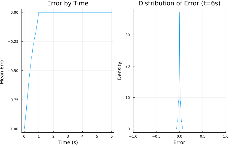
Figure 8: The mean amount of error between values calculated by a standard similarity operation and one operating via the interference of oscillators by time is shown (left). The distribution of these error values at the end of the simulation is narrow and centered on zero (right).

The difference in values output by the standard similarity function (2) and the oscillator-based similarity function (12) through time is displayed in Fig. 8. These similarity values fall on the real-valued domain $(-1,1]$. The error in similarity values decreases rapidly through time as input pulses transmitted to oscillators cause them to resonate with the correct phase. The complex potentials of these resonating oscillators are then interfered to obtain the correct similarity values with differences from the standard method remaining small and distributed around zero.

VI-B Bundling

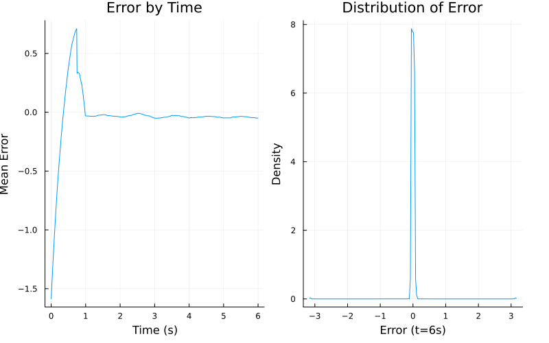
Figure 9: The mean amount of error between phase values produced by a standard bundling operation and one operating via the superposition of oscillator states is shown. This error decreases through time as the oscillators resonate with their input signals (left). The distribution of this error at the final simulation step is narrow and centered on zero (right).

The difference in phase values output by the standard bundling function (4) and the oscillator-based bundling function (13) are displayed in Fig. 9. Again, as the oscillators begin to resonate with their driving input signals, the superposition of their states produces the necessary outputs with small errors.

VI-C Binding

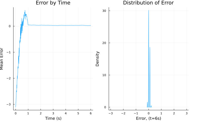
Figure 10: The mean amount of error between phase values produced by a standard binding operation and one operating via the multiplication of oscillator states is shown. As in the previous operations, this error decreases through time (left) and becomes narrowly centered around zero (right).

Lastly, this comparison is carried out for the binding operation, with the standard method (5) being used as the baseline against which the oscillator-based method (14) is compared. The error of the oscillator-based method again decreases through time and becomes small and centered on zero (Fig. 10).

VI-D Graph Compression

The previous experiments characterized the efficacy of FHRR computations implemented via oscillators on individual pairs of angles – these are the individual, atomic operations constituting the FHRR computing system. Next, we demonstrate these individual operations scaling up to hyperdimensional vectors and performed sequentially to carry out a task. The specific task we choose for this demonstration is the compression and reconstruction of graphs. This is accomplished by representing all edges contained within the graph with a single, HD symbol. Completing this task requires composing the previously demonstrated functions: binding, bundling, and similarity (as well as their inverse operations).

A series of undirected graphs with no self-loops were constructed via the Erdős–Rényi model. These graphs contain n nodes and a variable number of edges selected out of all possible pairs with probability p. Increasing p thus leads to an increase in the expected number of edges per graph.

These graphs can be represented in an HD space by selecting a set of random HD symbols, where each symbol uniquely corresponds to one node (22). In this experiment, each graph contained 25 nodes and each symbol representing a node contained 1,024 phase values.

$$node_{i}:=\bm{\phi}_{i}$$ (22)

To describe each edge in the graph, the symbols of the nodes adjacent to the edge can be bound to produce a new symbol (23).

$$edge_{i}=[node_{j}\Leftrightarrow node_{k}]:=bind(\bm{\phi}_{j},\bm{\phi}_{k})$$ (23)

This creates two sets of symbols: one representing the graph’s nodes, N, and the other representing its edges, E. The HD properties of these symbols makes it highly probable that each node symbol will be dissimilar to all others, and being derived from them, all edge symbols will be dissimilar to both the node symbols and other edge symbols. To reduce the amount of space needed to store the set of edges, it can be reduced via bundling to a single symbol (24)(Listing 1).

$$\bm{G}:=bundle(edge_{1},edge_{2},\ldots,edge_{m})$$ (24)

Listing 1: Compressing a graph’s edge structure into a single HD symbol

⬇

function compress_edges(graph):

#represent each node with an HD symbol

HD_nodes = rand_syms(length(graph.nodes))

HD_edges = []

for edge in graph.edges:

#produce a unique representation

# of each edge

source_index, destination_index = edge

HD_edge = bind(HD_nodes[source_index],

HD_nodes[destination_index])

append!(HD_edges, HD_edge)

end

#reduce the list of edges

# to a single symbol via bundling

HD_graph = bundle(HD_edges…)

return HD_nodes, HD_graph

This symbol $\bm{G}$ can be thought of as representing the list of edges in a graph in compressed form via HD operations. To reconstruct the graph’s adjacency matrix from this symbol, the set of symbols representing the nodes N is employed. For each node, its corresponding symbol is unbound from $G$ and the similarity of this product to all other nodes is calculated. This produces a matrix of similarity values (25)(Listing 2).

$$\begin{split}\bm{A}=[sim.(node_{j},unbind(\bm{A},node_{i}))]\\ fori\in 1:n,j\in 1:n,i\neq j\end{split}$$ (25)

Listing 2: Reconstructing a graph’s edges from a node symbols and a compressed edge symbol

⬇

function predict_edges(HD_nodes, HD_graph):

n_nodes = length(HD_nodes)

adjacency = zeros(n_nodes, n_nodes)

#unbind each node from the graph

# symbol to produce a key

for i in 1:n_nodes

source_node = HD_nodes[i]

key = unbind(HD_graph, source_node)

#measure the similarity between this key

# and another node

for j in 1:n_nodes

query = HD_nodes[j]

adjacency[i,j] = similarity(key, query)

end

end

return adjacency

All values in A above a certain threshold can be accepted as predicted true edges, and the rest as predicted false edges. This produces a classification which can be compared against the ground truth, which has an overall performance measured by the area under a receiver operating curve (AUROC).

This compression task increases with difficulty as more edges are included in the graph until a point of maximum entropy is reached. This is reflected in the trend of the performance of the reconstruction with increasing probability of edges in the graph for the conventional floating-point implementation (Fig. 11). The oscillator-based implementation begins with performance similar to the floating-point implementation, but degrades more quickly and shows increased variance. This is due to several factors, such as the fixed, discrete steps used in the solution to the system of equations which effectively limits values to a fixed-point representation and leads to errors in the output of operations shown previously.

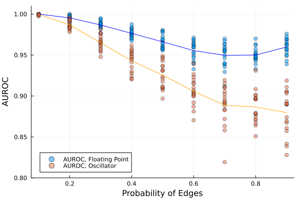
Figure 11: The performance of a classifier used to reconstruct graphs from a compressed representation was measured against an increase in the probability of edges in an Erdős–Rényi random graph. As the encoding process increases in complexity, the quality of the reconstruction determined from the HD embedding suffers. Executing this operation via oscillator-based computation as opposed to a floating-point implementation showed more significant decreases more quickly, demonstrating that small changes in the accuracy of HD operations can have significant impacts on performance.

VII Discussion

In the previous sections, we have demonstrated that HD computing operations can be carried out via a system of linked, ideal oscillators. While this provides a proof-of-concept for integrating devices into useful computational circuits, the practical feasibility of these systems must be evaluated.

On the level of individual devices, all oscillators contain non-idealities which affect their performance. For instance, no two physical oscillators are perfectly matched in frequency, though they can be driven to resonate in synchrony [29]. Physical oscillators also reach limits in their phase domain, such as the displacement achievable by the cantilever of a MEMS oscillator or the charge which can be stored in a resonant electronic circuit. All calculations carried out by the oscillator must be normalized within this phase space to avoid distortion or failure of components. Different components will also lead to changes in ease of fabrication, scalability, power dissipation, and accuracy of individual oscillator phases.

A circuit-level implementation of oscillatory HD computing would require thousands of oscillators in a circuit, with series of many oscillators dedicated to represent an HD symbol. The complex-valued information in these circuits must then be accessible to carry out addition, multiplication, inversion, and conjugation: the operations required for forwards and inverse bundling and binding, as well as similarity.

The ease of transporting this information and carrying out these operations changes greatly with the underlying physical implementation. For instance, coherent beams of light can be used to represent a phase, transported via waveguides, and summed via superposition. However, ‘multiplying’ two beams of light is not as simple to achieve, due to the lack of interaction between photons. While capacitive-inductive oscillators offer a similar appeal due to their ability to represent a system via two physical domains, the difficulty of integrating inductors into integrated circuits remains a challenge to their adoption in large-scale systems. Familiar electronic systems, such as CMOS, offer the highest scalability, ability to transport information, and efficient sub-threshold operation. However, the use of the electronic domain alone requires at least two transistors to represent a single oscillator and explicit addition and multiplication circuits which may be achievable by simpler, physical operations in other devices.

At the system level, the accuracy achieved by each operations must be high; our experiments suggest that small differences in the precision of operations can lead to significant impacts on the performance of a task. We observed that performance was highly dependent on parameters underlying the simulation of the oscillatory systems, such as the resolution of the temporal basis and the duration of the kernel being used to apply impulses to individual oscillators. Performance requirements may also change with the number of values composing an HD symbol, and may be applicable as a circuit-level trade-off to achieve higher accuracy using more components. Additionally, we have considered the case in which each oscillator produces a continuously-valued phase; restricting these values to finite subset would discretize the system, allowing it to carry out deterministic operations. Reducing the number of phase values would impact the overall performance of the system, but it should be noted that one HD computing system computes digitally with only two phase values [19].

Finally, success in computing requires an operation to be easily integrable with the dominant digital ecosystem. For many emergent computing operations such as computation-in-memory, this requires a conversion between the analog and digital domains which can ultimately be costly [11]. Analog, oscillatory HD computing systems would require efficient, scalable means of converting phases from their analog representations into digital values which can be stored and transported to other sections of a digital computer.

Utilizing detailed hardware models of oscillatory devices within the simulation framework is necessary to investigate the potential of oscillator-based HD computing systems at the device, circuit, and system level. However, the abundance of oscillatory devices such as subthreshold transistors, LC/RC circuits, MEMS cantilevers, spin torque oscillators, and coherent photonic systems suggests that there is already a rich field of devices and data which could be applied towards this objective [31].

For many extant tasks well-suited to digital logic, such as arithmetic and precise, repeatable calculations, HD computing systems are unlikely to provide competitive performance. However, for many other tasks such as interfacing with analog inputs, compressing noisy information in a structured manner, and manipulating and searching high-dimensional embeddings, HD computing is well-suited to provide useful approaches [22, 26, 32].

VIII Conclusion

Developing alternative methods of computation is crucial to addressing increasing demands as development of traditional approaches continues to increase in cost. In this work, we propose that hyperdimensional (HD) computing which represents information via vectors of phase angles provides a rich computational system with fundamental links to novel hardware devices. We provided proofs for the basis of this link and quantified via simulation the error in outputs of fundamental HD operations operating via systems of linked oscillators. These fundamental operations were applied to a graph compression task and its feasibility operating via oscillatory systems was verified. Finally, we suggest follow-up work investigating improving the accuracy of these oscillatory computations and establishing deeper links to specific classes of hardware devices.

References

- [1] N. Thompson, “The Economic Impact of Moore’s Law: Evidence from When it Faltered,” Ssrn, pp. 1–58, 2017, doi: 10.2139/ssrn.2899115.
- [2] J. L. Hennessy and D. A. Patterson, “A new golden age for computer architecture,” Commun. ACM, vol. 62, no. 2, pp. 48–60, Jan. 2019, doi: 10.1145/3282307.
- [3] W. Dally, “High-performance hardware for machine learning,” Nips Tutorial, vol. 2, p. 3, 2015.
- [4] “International Roadmap for Devices and Systems, 2022 Edition: Beyond CMOS and Emerging Materials Integration.” IEEE, 2022. [Online]. Available: https://irds.ieee.org/editions/2022/irds
- [5] X. Xu et al., “11 TOPS photonic convolutional accelerator for optical neural networks,” Nature, vol. 589, no. 7840, pp. 44–51, 2021, doi: 10.1038/s41586-020-03063-0.
- [6] S. Hooker, “The hardware lottery,” Communications of the ACM, vol. 64, no. 12, pp. 58–65, 2021, doi: 10.1145/3467017.
- [7] D. Kleyko, D. A. Rachkovskij, E. Osipov, and A. Rahimi, “A Survey on Hyperdimensional Computing aka Vector Symbolic Architectures, Part I: Models and Data Transformations,” pp. 1–27, 2021.
- [8] Y. E. Wang, G.-Y. Wei, and D. Brooks, “Benchmarking TPU, GPU, and CPU Platforms for Deep Learning.” arXiv, Oct. 22, 2019. Accessed: Sep. 11, 2023. [Online]. Available: http://arxiv.org/abs/1907.10701
- [9] M. Emani et al., “A Comprehensive Evaluation of Novel AI Accelerators for Deep Learning Workloads,” in 2022 IEEE/ACM International Workshop on Performance Modeling, Benchmarking and Simulation of High Performance Computer Systems (PMBS), Dallas, TX, USA: IEEE, Nov. 2022, pp. 13–25. doi: 10.1109/PMBS56514.2022.00007.
- [10] S. Yu, H. Jiang, S. Huang, X. Peng, and A. Lu, “Compute-in-Memory Chips for Deep Learning: Recent Trends and Prospects,” IEEE Circuits Syst. Mag., vol. 21, no. 3, pp. 31–56, 2021, doi: 10.1109/MCAS.2021.3092533.
- [11] A. Amirsoleimani et al., “In‐Memory Vector‐Matrix Multiplication in Monolithic Complementary Metal–Oxide–Semiconductor‐Memristor Integrated Circuits: Design Choices, Challenges, and Perspectives,” Advanced Intelligent Systems, vol. 2, no. 11, p. 2000115, Nov. 2020, doi: 10.1002/aisy.202000115.
- [12] A. Reuther, P. Michaleas, M. Jones, V. Gadepally, S. Samsi, and J. Kepner, “AI Accelerator Survey and Trends,” 2021 IEEE High Performance Extreme Computing Conference, HPEC 2021, pp. 1–9, 2021, doi: 10.1109/HPEC49654.2021.9622867.
- [13] Gupta, Geetika, “What’s the Difference Between Single-, Double-, Multi- and Mixed-Precision Computing?,” NVIDIA. [Online]. Available: https://blogs.nvidia.com/blog/2019/11/15/whats-the-difference-between-single-double-multi-and-mixed-precision-computing/
- [14] Kharya, Paresh, “TensorFloat-32 in the A100 GPU Accelerates AI Training, HPC up to 20x,” NVIDIA. [Online]. Available: https://blogs.nvidia.com/blog/2020/05/14/tensorfloat-32-precision-format/
- [15] D. Kleyko et al., “Vector Symbolic Architectures as a Computing Framework for Nanoscale Hardware,” pp. 1–28, 2021.
- [16] J. Orchard and R. Jarvis, “Hyperdimensional Computing with Spiking-Phasor Neurons.” arXiv, Feb. 28, 2023. Accessed: Mar. 29, 2023. [Online]. Available: http://arxiv.org/abs/2303.00066
- [17] P. Kanerva, “Hyperdimensional computing: An introduction to computing in distributed representation with high-dimensional random vectors,” Cognitive Computation, vol. 1, no. 2, pp. 139–159, 2009, doi: 10.1007/s12559-009-9009-8.
- [18] P. Neubert, S. Schubert, and P. Protzel, “An Introduction to Hyperdimensional Computing for Robotics,” KI - Künstliche Intelligenz, vol. 33, no. 4, pp. 319–330, 2019, doi: 10.1007/s13218-019-00623-z.
- [19] K. Schlegel, P. Neubert, and P. Protzel, “A comparison of Vector Symbolic Architectures,” 2020, [Online]. Available: http://arxiv.org/abs/2001.11797
- [20] T. A. Plate, “Holographic reduced representations,” IEEE Transactions on Neural networks, vol. 6, no. 3, pp. 623–641, 1995.
- [21] T. A. Plate, Holographic Reduced Representation: Distributed Representation for Cognitive Structures. Center for the Study of Language and Information, 2003.
- [22] D. Kleyko, D. A. Rachkovskij, E. Osipov, and A. Rahimi, “A Survey on Hyperdimensional Computing aka Vector Symbolic Architectures, Part II: Applications, Cognitive Models, and Challenges,” pp. 1–36, 2021.
- [23] W. Olin-Ammentorp and M. Bazhenov, “Deep Phasor Networks: Connecting Conventional and Spiking Neural Networks,” Institute of Electrical and Electronics Engineers (IEEE), Sep. 2022, pp. 1–10. doi: 10.1109/ijcnn55064.2022.9891951.
- [24] W. Olin-Ammentorp and M. Bazhenov, “Residual and Attentional Architectures for Vector-Symbols.”
- [25] C. Bybee, E. P. Frady, and F. T. Sommer, “Deep Learning in Spiking Phasor Neural Networks.” arXiv, Apr. 01, 2022. Accessed: Jan. 09, 2023. [Online]. Available: http://arxiv.org/abs/2204.00507
- [26] E. P. Frady and F. T. Sommer, “Robust computation with rhythmic spike patterns,” Proceedings of the National Academy of Sciences, vol. 116, no. 36, pp. 18050–18059, 2019, doi: 10.1073/pnas.1902653116.
- [27] S. J. Kent, E. P. Frady, F. T. Sommer, and B. A. Olshausen, “Resonator Circuits for factoring high-dimensional vectors,” pp. 1–61, 2019.
- [28] E. P. Frady, S. Kent, B. A. Olshausen, and F. T. Sommer, “Resonator networks for factoring distributed representations of data structures,” pp. 1–20, 2020.
- [29] A. Pikovsky, M. Rosenblum, and J. Kurths, “Synchronization: A universal concept in nonlinear sciences,” Self, vol. 2, p. 3, 2001.
- [30] E. M. Izhikevich, “Resonate-and-fire neurons,” Neural Networks, vol. 14, no. 6–7, pp. 883–894, 2001, doi: 10.1016/S0893-6080(01)00078-8.
- [31] G. Csaba and W. Porod, “Coupled oscillators for computing: A review and perspective,” Applied Physics Reviews, vol. 7, no. 1, 2020, doi: 10.1063/1.5120412.
- [32] M. Imani, A. Rahimi, D. Kong, T. Rosing, and J. M. Rabaey, “Exploring Hyperdimensional Associative Memory,” in 2017 IEEE International Symposium on High Performance Computer Architecture (HPCA), Austin, TX: IEEE, Feb. 2017, pp. 445–456. doi: 10.1109/HPCA.2017.28.