Clustering Mixtures of Bounded Covariance Distributions
Under Optimal Separation

Abstract

We study the clustering problem for mixtures of bounded covariance distributions, under a fine-grained separation assumption. Specifically, given samples from a $k$-component mixture distribution $D=\sum_{i=1}^{k}w_{i}P_{i}$, where each $w_{i}\geq\alpha$ for some known parameter $\alpha$, and each $P_{i}$ has unknown covariance $\Sigma_{i}\preceq\sigma^{2}_{i}\cdot I_{d}$ for some unknown $\sigma_{i}$, the goal is to cluster the samples assuming a pairwise mean separation in the order of $(\sigma_{i}+\sigma_{j})/\sqrt{\alpha}$ between every pair of components $P_{i}$ and $P_{j}$. Our main contributions are as follows:

• For the special case of nearly uniform mixtures, we give the first polynomial-time algorithm for this clustering task. Prior work either required separation scaling with the maximum cluster standard deviation (i.e. $\max_{i}\sigma_{i}$) [DKK⁺22b] or required both additional structural assumptions and mean separation scaling as a large degree polynomial in $1/\alpha$ [BKK22].

• For arbitrary (i.e. general-weight) mixtures, we point out that accurate clustering is information-theoretically impossible under our fine-grained mean separation assumptions. We introduce the notion of a clustering refinement — a list of not-too-small subsets satisfying a similar separation, and which can be merged into a clustering approximating the ground truth — and show that it is possible to efficiently compute an accurate clustering refinement of the samples. Furthermore, under a variant of the “no large sub-cluster” condition introduced in prior work [BKK22], we show that our algorithm will output an accurate clustering, not just a refinement, even for general-weight mixtures. As a corollary, we obtain efficient clustering algorithms for mixtures of well-conditioned high-dimensional log-concave distributions.

Moreover, our algorithm is robust to a fraction of adversarial outliers comparable to $\alpha$.

At the technical level, our algorithm proceeds by first using list-decodable mean estimation to generate a polynomial-size list of possible cluster means, before successively pruning candidates using a carefully constructed convex program. In particular, the convex program takes as input a candidate mean $\hat{\mu}$ and a scale parameter $\hat{s}$, and determines the existence of a subset of points that could plausibly form a cluster with scale $\hat{s}$ centered around $\hat{\mu}$. While the natural way of designing this program makes it non-convex, we construct a convex relaxation which remains satisfiable by (and only by) not-too-small subsets of true clusters.

1 Introduction

Clustering mixture models is one of the most basic and widely-used statistical primitives on data samples from high-dimensional distributions, with applications in a variety of fields, including bioinformatics, astrophysics, and marketing [Lin95, GEGMMI10]; see [TSM85] for an extensive list of applications. Informally, the input is a set of $n$ samples drawn from a mixture distribution $D=\sum_{i=1}^{k}w_{i}P_{i}$ over $\mathbb{R}^{d}$, where $w_{i}$ is the mixing weight of component $P_{i}$. The goal is to cluster (most of) the samples such that the clustering is approximately equal to partitioning the data according to the ground truth; namely, partitioning samples according to which mixture component they were drawn from. For the clustering task to be information-theoretically possible, it is common to make concentration assumptions on each mixture component $P_{i}$ (e.g. sub-Gaussianity, or a bounded moments assumption), as well as on the pairwise separation between the means of the components.

The prototypical case is that of Gaussian mixtures and has been extensively studied in the literature; see, e.g. [VW02, KSV05, AM05] and references therein. In more detail, [VW02] studied the clustering of data drawn from mixtures of separated spherical Gaussians. Subsequent work [KSV05, AM05] built on the approach of [VW02] to design clustering algorithms for mixtures of separated Gaussians with general covariances. The main algorithmic technique underlying these papers is to apply $k$-PCA in order to discover the subspace spanned by the means of the mixture components.

The focus of this paper is the more general heavy-tailed setting, where each component is only assumed to have bounded covariance instead of stronger concentration. Specifically, suppose that each component $P_{i}$ has unknown covariance matrix $\Sigma_{i}$ that satisfies $\Sigma_{i}\preceq\sigma^{2}\cdot I_{d}$, for some unknown parameter $\sigma>0$. For notational simplicity, we restrict this discussion to uniform mixtures (corresponding to the case that $w_{i}=1/k$ for all $i\in[k]$). Then, unless the component means have pairwise $\ell_{2}$-distance $\gg\sigma\sqrt{k}$, accurate clustering is information-theoretically impossible in the worst-case. On the positive side, the recent work of [DKK⁺22b] gave a computationally efficient algorithm which achieved the best worst-case separation: if all the components $P_{i}$ have covariances $\Sigma_{i}\preceq\sigma^{2}\cdot I_{d}$, then [DKK⁺22b] showed that it is possible to accurately cluster when given a pairwise separation of $C\sigma\sqrt{k}$, where $C>0$ is a sufficiently large universal constant.

The preceding discussion suggests that the algorithmic problem of clustering mixtures of bounded covariance distributions under the information-theoretically optimal mean estimation (within constant factors) is fully resolved. Yet, consider the simple example shown in Figure 1 below.

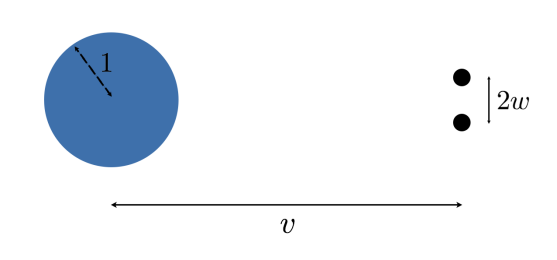
Figure 1: Example “well-separated” mixture distribution that cannot be handled by the algorithm of [DKK⁺22b].

In this example, we have an identity-covariance distribution on the left, separated by distance $v\gg 1$ from a pair of $0$-covariance distributions on the right, which are in turn separated by some small distance $2w\ll 1$. This example is clearly clusterable and “well-separated”, since there is essentially no overlap between any of the mixture components. However, the example cannot be handled by the algorithm of [DKK⁺22b] or earlier algorithms for the following reason: the largest variance is $\sigma^{2}=1$, but the two $0$-covariance distributions are separated only by $2w\ll 1$ — instead of the required $\Theta(\sigma\sqrt{k})=\Theta(1)$ separation.

The above example illustrates an important conceptual weakness of prior work in the heavy-tailed (bounded covariance) setting: it requires that the pairwise mean separation is measured by the maximum covariance across all the mixture components — even if the pair of components in question both have small covariances. This distinction can make a large quantitative difference in both theory and practice. Indeed, even for the special case that the components are of approximately the same size (cardinality), their relative radii may dramatically differ.

Motivation: Achieving fine-grained separation

A more reasonable separation assumption that we focus on in this paper is as follows. Suppose that the components $P_{i}$ and $P_{j}$ have maximum standard deviations $\sigma_{i}$ and $\sigma_{j}$ respectively. Then we require the corresponding means $\mu_{i}$ and $\mu_{j}$ to be separated in $\ell_{2}$-distance by a quantity scaling with $\sigma_{i}+\sigma_{j}$. Note that this is much weaker than the prior assumption scaling with $\max_{i}\sigma_{i}$. We also point out that clustering under such fine-grained separation has been achieved for Gaussian components in earlier works [AM05, KSV05, Bru09]. However, to the best of our knowledge, no such result was previously known for the bounded covariance setting. Motivated by this gap in the literature, in this paper we ask:

Is it possible to efficiently cluster data from mixtures of bounded covariance distributions under the fine-grained separation assumption? Specifically, can we efficiently achieve accurate clustering under pairwise mean separation in the order of $\sqrt{k}(\sigma_{i}+\sigma_{j})$?

As our main contribution, in this paper we study and essentially resolve this question.

We emphasize that the heavy-tailed setting introduces a number of technical challenges that do not appear in the presence of strong concentration. For the sake of intuition, we explain below how $k$-PCA — a standard spectral technique used in prior work — provably fails in our setting.

Failure of $k$-PCA

One of the main standard techniques for clustering mixtures of separated components is to perform $k$-PCA: find the top-$k$ dimensional subspace of the sample covariance, and show that with high probability, this subspace captures the span of the mixture component means. However, this technique fails for bounded covariance distributions under our fine-grained separation assumption, even with infinitely many samples. This can be demonstrated through a variant of the example in Figure 1. Consider the uniform (i.e. equal weights) mixture with a component with unit covariance on a subspace $V$ at the origin, and two components with $0$-covariance, located at points $v+w$ and $v-w$ with $\|v\|_{2}\gg 1$ and $\|w\|_{2}\ll 1$. Suppose also that $V$ is $\Omega(d)$-dimensional, and $V,v,w$ are orthogonal to each other. Denoting the identity matrix in the subspace $V$ by $I_{V}$, the covariance of the full distribution is equal to $\frac{1}{3}I_{V}+\frac{2}{9}vv^{\top}+\frac{2}{3}ww^{\top}$. Given that $\|v\|_{2}\gg 1$ and $\|w\|_{2}\ll 1$, the eigenvectors of this covariance are $v$, any $\Omega(d)$-dimensional basis of $V$, finally followed by $w$. Thus, in order to have the direction $w$ in the subspace found by $k$-PCA, we might need as many as $k=\Omega(d)$ dimensions, which reduces the dimensionality only mildly.

Summary of contributions

Our first goal focuses on uniform-weight mixture distributions, with the aim of clustering assuming only a pairwise separation of $C\cdot(\sigma_{i}+\sigma_{j})\sqrt{k}$ between mixture components $P_{i}$ and $P_{j}$ satisfying $\Sigma_{i}\preceq\sigma^{2}_{i}\cdot I_{d}$ and $\Sigma_{j}\preceq\sigma^{2}_{j}\cdot I_{d}$, for some sufficiently large universal constant $C$. We note that the individual standard deviations $\sigma_{i}$ are unknown to the algorithm.

For this setting, we give the first efficient algorithm (Algorithm 1) achieving this guarantee in Theorem 1.1. We point out that the recent work of [BKK22] also studies the heavy-tailed setting under a fine-grained separation assumption. However, they require separation which scales like $(\sigma_{i}+\sigma_{j})\operatorname*{\mathrm{poly}}(k,\log n)$, for a large degree polynomial. More importantly, they also require an additional “no large sub-cluster assumption” on the samples beyond bounded covariance — even for the uniform-weight mixture setting.

Our second, more general goal is to study the limits of clustering general-weight mixtures of bounded covariance distributions, under the same fine-grained pairwise separation assumption. Perhaps surprisingly, we point out that it is information-theoretically impossible to achieve accurate clustering due to identifiability issues — there can be multiple valid ground truths for the same mixture and there is no way to tell which one is the “correct” one — if the mixing weights are (highly) non-uniform. Nonetheless, our main algorithm (Algorithm 1) efficiently produces an accurate refinement of the ground truth clustering (Theorem 1.4): informally, a clustering refinement is a list of not-too-small and disjoint subsets of samples such that there exists a way to combine them into a clustering close to the ground truth, and furthermore, these subset are themselves well-separated like the ground truth distribution. This essentially amounts to the information-theoretically strongest possible guarantee in our setting. We further show that, under a “no large sub-cluster” condition (à la [BKK22]), the same algorithm outputs exactly the correct $k$ clusters (up to some small fraction of misclassified points).

Finally, we remark that our algorithm is robust to a fraction of adversarial outliers that is comparable to the size of the smallest cluster.

1.1 Our results

Even in the special case of uniform-weight mixtures, no prior work can find an accurate clustering under a fine-grained separation assumption scaling with $\sigma_{i}+\sigma_{j}$ between components $P_{i}$ and $P_{j}$, even if we allow a sub-optimal $\operatorname*{\mathrm{poly}}(k)$ scaling. Here we present our first result, solving both issues simultaneously. Algorithm 1 finds an accurate clustering in polynomial time, assuming the optimal (up-to-constants) separation in the order of $(\sigma_{i}+\sigma_{j})\sqrt{k}$, which is both fine-grained and has the information-theoretically optimal $\sqrt{k}$ dependence.

Theorem 1.1 (Clustering uniform-weight bounded covariance mixtures).

Let $C$ be a sufficiently large constant. Consider a uniform-weight mixture distribution $D=\sum_{i=1}^{k}\frac{1}{k}P_{i}$ with $k$ components on $\mathbb{R}^{d}$. Suppose that $\alpha$ is a parameter in $[0.6/k,1/k]$. Let $\mu_{i}$ and $\Sigma_{i}$ be the (unknown) mean and covariance of each $P_{i}$, and assume that $\Sigma_{i}\preceq\sigma_{i}^{2}\cdot I_{d}$ (with $\sigma_{i}$ being unknown) and $\|\mu_{i}-\mu_{j}\|_{2}>C(\sigma_{i}+\sigma_{j})/\sqrt{\alpha}$ for all $i\neq j$.

Draw $n$ samples from $D$, and let $S_{i}$ be the samples from the $i^{\text{th}}$ mixture component. Further fix a failure probability $\delta>0$. If $n>C(d\log(d)+\log(1/(\alpha\delta)))/\alpha^{2}$, then Algorithm 1 when given the samples, $\alpha,$ and $\delta$ as input, runs in polynomial time and outputs $k$ disjoint sets $\{B_{i}\}_{i\in k}$ so that with probability at least $1-\delta$ the following are true, up to a permutation of indices of the output sets:

1. $|S_{i}\triangle B_{i}|\leq 0.045n/k$ for every $i\in[k]$.

2. The mean of $B_{i}$ is close to $S_{i}$: $\|\mu_{B_{i}}-\mu_{i}\|_{2}=O(\sigma_{i})$ for every $i\in[k]$.

Algorithm 1 is given as input a minimum-weight parameter $\alpha\in[0.6/k,1/k]$, and in polynomial-time it returns a list of exactly $k$ sets, $\{B_{i}\}$, such that, up to a permutation, each $B_{i}$ has a 95% overlap with the set $S_{i}$ of samples drawn from the $i^{\text{th}}$ mixture component $P_{i}$ and that the mean $\mu_{B_{i}}$ of $B_{i}$ is indeed close to the mean $\mu_{i}$ of $P_{i}$, under the minimal assumption that the means of the $i^{th}$ and $j^{th}$ clusters are separated by at least a large constant multiple of $(\sigma_{i}+\sigma_{j})/\sqrt{\alpha}$. We note that i) the 95% overlap can be made an arbitrarily close constant to 1 by increasing the hidden constant in the separation assumption and adapting corresponding constants in the algorithm, and ii) we do not require any “no large sub-cluster condition” in the uniform mixture setting.

We also stress that Algorithm 1 does not require knowing $k$ precisely, and only needs to know a lower bound $\alpha$ for $1/k$, which can be a (small) constant factor different.

We further remark that Item 1 above lower bounds the size of the union of all the $B_{i}$s by $0.95n$, namely that at least 95% of all the points are clustered and returned. As noted above, the 95% can be made into any constant arbitrarily close to 100%, by increasing the constant $C$ in the separation assumption. Alternatively, if we drop Item 2 in the theorem statement, namely that the requirement that the mean of $B_{i}$ is indeed close to the mean $\mu_{i}$ of component $P_{i}$, then it is possible to return all the input samples in the output clustering.

Moreover, Theorem 1.1 holds even for almost-uniform mixtures, where each mixing weight $w_{i}\in[0.9/k,1.1/k]$, and if $\alpha\in[0.7/k,\min_{i}w_{i}]$.

The situation of general (non-uniform) mixing weights is somewhat more complicated. For example, in the situation described below (also shown in Figure 2), even if we know the number $k$ of components and even if we have infinitely many samples, it is information-theoretically impossible to reliably achieve a 90%-accurate clustering.

Example: Non-identifiability of general mixtures

Consider a distribution consisting of 4 equal weight 0-covariance components, separated into 2 pairs. Each pair is at unit distance, and the two pairs are separated by a large distance. Suppose we are given that $k=3$ and $\alpha=1/4$, then there are two possible clusterings that disagree with each other by at least 25% of the total mass: either group the first pair as a large cluster with weight $1/2$ and leave the second pair as two smaller clusters, or by symmetry we can group the second pair instead. It is allegorically impossible to determine which of these is the “true” ground truth clustering even with infinitely many samples from the mixture.

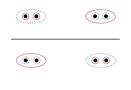
Figure 2: Two different ground truth clusterings for $k=3$.

Given the above impossibility example, the question remains, what is possible given only the mixing weight lower bound parameter $\alpha$, and a separation assumption of $C(\sigma_{i}+\sigma_{j})/\sqrt{\alpha}$ between components $P_{i}$ and $P_{j}$? The example highlights the core of the non-identifiability issue: an impossibility to identify which small subsets to group together. Consequently, we can perhaps hope to compute all the information in the ground truth clustering except for such subset grouping. That is, we can try to identify only the small subsets themselves. Motivated by this observation, we instead aim to return a refinement of the clustering: we will return a list of $\geq k$ subsets (which we will call sub-clusters), each of size at least $\approx\alpha n$, such that there exists some way of grouping the subsets into $k$ larger clusters which then correspond to the ground truth mixture distribution.

For example, in the concrete setting of Figure 2, we could return the 4 small sub-clusters individually, which is a common refinement of the two possible clusterings shown in the figure. Furthermore, (as we will show) we can even guarantee that the returned subsets satisfy a pairwise separation guarantee similar to what we assume of our underlying mixture distribution.

Our main result (Theorem 1.4) of the paper shows that it is indeed possible to find an accurate refinement of the ground truth clustering, using $\tilde{O}(d/\alpha^{2})$ samples and in polynomial time, with Algorithm 1. We define an accurate refinement below, as well as state a simplified version of our main theorem.

Definition 1.2 (Accurate refinement of ground truth clustering).

Let $c>0$ be an absolute constant. Suppose we draw $n$ samples from the mixture distribution $D=\sum_{i=1}^{k}w_{i}P_{i}$, where each $w_{i}\geq\alpha$ and each $P_{i}$ has mean $\mu_{i}$ and standard deviation $\sigma_{i}$. Let $S_{i}$ be the set of samples drawn from $P_{i}$.

An accurate refinement of the clustering $S_{i}$ is a list of $m$ disjoint sets of samples $\{B_{j}\}_{j\in[m]}$ for some $m\in[k,O(1/\alpha)]$, such that:

1. The sets $B_{1},\ldots,B_{m}$ each have size $|B_{j}|\geq 0.92\alpha n$ for all $j\in[m]$.

2. The indices $[m]$ can be partitioned into $k$ sets $H_{1},\ldots,H_{k}$, such that if $\mathcal{B}_{i}$ are defined as $\mathcal{B}_{i}:=\cup_{j\in H_{i}}B_{j}$, the following hold:

   1. $|{S}_{i}\setminus\mathcal{B}_{i}|\leq 0.045|{S}_{i}|$ for every $i\in[k]$.

   2. $|\mathcal{B}_{i}\setminus{S}_{i}|\leq 0.03\alpha n$ for every $i\in[k]$.

   3. For any $i\in[k]$ and any $j\in H_{i}$ we have that $\|\mu_{B_{j}}-\mu_{i}\|_{2}\leq c\,\sigma_{i}\sqrt{|{S}_{i}|/|B_{j}|}$.

   4. For any pair $j\neq j^{\prime}$ we have that $\|\mu_{B_{j}}-\mu_{B_{j^{\prime}}}\|_{2}>100\,c\,(\sigma_{B_{j}}+\sigma_{B_{j^{\prime}}})/\sqrt{\alpha}$, where $\sigma_{B_{j}}$ is the maximum standard deviation of $B_{j}$.

3. As a consequence of Item 2a we have that $|\cup_{j\in[m]}B_{j}|\geq 0.95n$, namely that 95% of the input points are classified into the output sets.

Item 1 above says that each returned set must have size at least $\approx\alpha n$, given that each mixture component is supposed to have weight at least $\alpha$. Item 2 captures the core idea of a refinement: there exists some way to combining the returned sets into sets $\mathcal{B}_{1},\ldots,\mathcal{B}_{k}$, each corresponding to a mixture component $P_{1},\ldots,P_{k}$, with the following guarantees. Items 2a and 2b say that the symmetric difference between the samples $S_{i}$ drawn from component $P_{i}$ and the set $\mathcal{B}_{i}$ is small. Item 2c says that each output set $B_{j}$ must be close to the true mean of its corresponding mixture component $P_{i}$, with error scaling with $\sigma_{i}$ as well as $\sqrt{|S_{i}|/|B_{j}|}$ — the larger $B_{j}$ is, containing more samples in $S_{i}$, the closer $\mu_{B_{j}}$ should be to $\mu_{i}$. Item 2d says that the returned subsets $\{B_{j}\}$ must themselves satisfy a mean separation akin to the one satisfied by the mixture components, up to a constant factor loss. Lastly, Item 3 guarantees that at least $95\%$ of the samples are indeed classified and returned in one of the output sets.

Remark 1.3.

The guarantees of Definition 1.2 imply that for every output set $B_{j}$ there exists a true cluster $S_{i}$ such that $|B_{j}\cap S_{i}|=|B_{j}|-|B_{j}\setminus S_{i}|\geq|B_{j}|-|\mathcal{B}_{i}\setminus S_{i}|\geq|B_{j}|-0.03\alpha n\geq(1-0.03/0.92)|B_{j}|\geq 0.967|B_{j}|$, i.e. more than $96\%$ of the points in the output set come from the true cluster $S_{i}$.

Theorem 1.4 (Simplified version of Theorem 3.1).

Consider a mixture distribution on $\mathbb{R}^{d}$, $D=\sum_{i=1}^{k}w_{i}P_{i}$ with unknown positive weights $w_{i}\geq\alpha$ for some known parameter $\alpha\in(0,1)$. Let $\mu_{i}$ and $\Sigma_{i}$ be the (unknown) mean and covariance for each $P_{i}$, and assume that $\Sigma_{i}\preceq\sigma_{i}^{2}\cdot I_{d}$ for all $i\in[k]$ (with $\sigma_{i}$ being unknown) and $\|\mu_{i}-\mu_{j}\|_{2}>C(\sigma_{i}+\sigma_{j})/\sqrt{\alpha}$ for every $i\neq j$, for a sufficiently large constant $C$.

There is an algorithm (Algorithm 1) which, when given $\alpha$ and $n$ independent samples from $D$ for $n$ at least a sufficiently large multiple of $(d\log d+\log(1/(\alpha\delta)))/\alpha^{2}$, runs in polynomial time and with probability at least $1-\delta$ (over the randomness of both the samples and the algorithm), outputs an accurate refinement clustering of these samples in the sense of Definition 1.2.

As in Theorem 1.1, for Definition 1.2 to be satisfied by the algorithm output, we can make the constant 0.92 in Item 1 arbitrarily close to $1$, and the constants in Items 2a and 2b arbitrarily close to 0, if we increased the constant in the mean separation assumption in Theorem 1.4.

We also remark that the same algorithm (Algorithm 1) can even tolerate adversarial corruption in an $\Omega(\alpha)$-fraction of the samples. See the full theorem, Theorem 3.1, for the detailed statement.

Clustering under “no large sub-clusters”

We can further guarantee that Algorithm 1 returns only $k$ clusters (thereby corresponding exactly to the $k$ ground truth components), if we also assume a “no large sub-cluster” condition à la [BKK22], stated in Definition 1.5. Informally, the condition says that for any large subset $S^{\prime}$ of samples $S_{i}$ drawn from the $i^{\text{th}}$ mixture component, the standard deviation $\sigma_{S^{\prime}}$ of $S^{\prime}$ is comparable to $\sigma_{S_{i}}$. This is intuitively the contrapositive of not having any large sub-clusters: a large sub-cluster can be understood as a large subset that is separated from the rest of the clusters, meaning that it has a substantially smaller covariance. Our condition below is qualitatively the same condition as that of [BKK22], but with a stronger quantitative requirement on the parameters of a sub-cluster. In Section 8.1, we show that such a stronger condition is information-theoretically necessary, due to our much weaker (and optimal) mixture separation assumption. Afterwards, in Section 8.2, we also show (see Corollary 1.6, an informal version of Corollary 8.2), that if the condition is satisfied, then there can only be one possible ground truth (i.e., there are no identifiability issues anymore) and thus Algorithm 1 indeed returns only one output set per real mixture component.

Definition 1.5 (NLSC condition).

We say that the disjoint sets $S_{1},\ldots,S_{k}$ of total size $n$ satisfy the “No Large Sub-Cluster” condition with parameter $\alpha$ if for any cluster $S_{i}$ and any subset $S^{\prime}\subset S_{i}$ with $|S^{\prime}|\geq 0.8\alpha n$, it holds that $\sigma_{S^{\prime}}\geq 0.1\sigma_{S_{i}}$, where $\sigma_{S^{\prime}}$ is the square root of the largest eigenvalue of the covariance matrix of $S^{\prime}$.

Corollary 1.6 (Informal version of Corollary 8.2).

If the samples $S_{i}$ from the $i^{\text{th}}$ mixture component jointly satisfy the NLSC assumption with parameter $\alpha$ across all $i\in[k]$, then Algorithm 1 returns exactly one sample set per mixture component (with high probability). As a consequence, if $B_{i}$ is the output set corresponding to the $i^{\text{th}}$ mixture component, then we have $\|\mu_{B_{i}}-\mu_{i}\|\leq O(\sigma_{i})$, just like in Theorem 1.1.

Later in Section 8.2, we also show that well-conditioned and high-dimensional log-concave distributions have samples that satisfy the NLSC condition with high probability. We remark that the high-dimensionality assumption is necessary: the thin-shell behavior of log-concave distributions in high dimensions is critical to satisfy our NLSC condition.

Proposition 1.7 (Informal version of Proposition 8.5).

A sample of size $\tilde{O}(d/\alpha^{2})$ drawn from a well-conditioned and high-dimensional log-concave distribution satisfies the NLSC condition (Definition 1.5) with high probability.

Before moving on to an overview of our algorithmic techniques, we emphasize that, even though we presented multiple results in multiple settings (uniform vs general weight mixtures, with and without the NLSC condition), they all apply to the same algorithm without needing any changes even in the hardcoded constants. Algorithm 1 does not need any knowledge of whether any of the conditions hold; it achieves the corresponding results automatically whenever the corresponding assumptions are satisfied.

1.2 Technical overview

In this section, we give an overview of the components and techniques used in Algorithm 1, our main algorithm.

Since the mixture component means are assumed to be well-separated, Algorithm 1 works by finding a list of candidate mean vectors, each of which is close to a mixture component, with the entire list “covering” all the components. Once we have such a list, it suffices to consider the Voronoi partition of the samples; that is, to assign each point to the cluster of the closest candidate mean. The mean separation assumption, along with the concentration of bounded covariance distributions, guarantee that such a Voronoi partition will be close to a refinement of the ground truth clustering.

The high-level idea of finding such a list of candidate mean vectors is to first generate a much larger (but still polynomially-sized) list which potentially contains candidates that are far from all mixture components, and then prune all the invalid candidate means out of the list. The first part is relatively straightforward, since there are standard list-decodable mean estimation algorithms for bounded-covariance distributions (e.g. [DKK⁺21]). The only minor complication is that, for these algorithms to return means with tight error guarantees, they need good upper bounds on the standard deviation of each mixture component. We thus first generate a list of possible standard deviations $\hat{s}$ (Proposition 2.7), and for each $\hat{s}$, run the list-decodable mean estimation algorithm. After this step, we have a list of candidate means such that, for each mixture component, there is at least one candidate mean close to it.

The next step is at the heart of our algorithm: to prune candidate means that are not sufficiently close to any mixture component (with distance threshold scaling with the standard deviation of the mixture component). A natural way to do this would be to test each candidate mean by trying to find its corresponding cluster and seeing if that exists. In particular, given a candidate mean $\hat{\mu}$ and candidate standard deviation $\hat{s}$, we would like to find a subset of at least an $\approx\alpha$-fraction of the samples whose covariance matrix is bounded by $O(\hat{s}^{2})\cdot I_{d}$ and whose mean is within $O(\hat{s}/\sqrt{\alpha})$ of $\hat{\mu}$. If we can find this, it suggests that the cluster we are looking for actually exists.

Unfortunately, the natural approach of finding such a cluster is computationally hard, so we need to find appropriate relaxations to make it tractable. Immediately, to avoid computational hardness from integrality issues, we begin by allowing a weighted subset rather than an actual subset, which concretely is to find weights $w_{i}\in[0,1]$ over each sample $x_{i}$, such that $\sum_{i}w_{i}$ is at least $\approx\alpha n$. This nearly turns our problem into a convex program. In particular, if we knew the mean of the cluster exactly, the covariance would be a linear function of $\{w_{i}\}_{i}$, making it a convex program. However, as we do not know the real mean, the covariance matrix centered at $\mu_{w}$ — the mean of the weighted cluster defined by $\{w_{i}\}_{i}$ — is no longer linear in $\{w_{i}\}_{i}$, and the constraint bounding its operator norm is no longer a convex constraint. So, instead, we compute the second moment matrix of $\{w_{i}\}_{i}$ centered at the candidate mean $\hat{\mu}$ (i.e. proportional to $\sum_{i}w_{i}(x_{i}-\hat{\mu})(x_{i}-\hat{\mu})^{\top}$). This gives us a convex program, but unfortunately one that might not be satisfiable even by a correct cluster $C$ whose mean is indeed $O(\hat{s}/\sqrt{\alpha})$ close to the candidate mean $\hat{\mu}$: the second moment matrix of $C$ would actually be $\operatorname*{\mathrm{Cov}}(C)+(\hat{\mu}-\mu_{C})(\hat{\mu}-\mu_{C})^{\top}$, and the latter term might contribute to an eigenvector of size as large as $\Omega(\hat{s}^{2}/\alpha)$, which is too large when $\alpha$ is small. We must therefore further relax our convex program. Instead of finding $\{w_{i}\}$ whose second moment matrix centered at $\hat{\mu}$ has operator norm bounded by $O(\hat{s}^{2})\cdot I_{d}$, we constrain its $O(1/\alpha)$-Ky-Fan norm by $O(\hat{s}^{2}/\alpha)$. This new, final program (Program (1) in Section 4) is now both convex and satisfiable by a true cluster.

The next obstacle, however, is that a solution $\{w_{i}\}_{i}$ to the above convex program might not actually correspond to a true cluster or mixture component. In particular, if there are other clusters with standard deviation much smaller than $\hat{s}$, we might have found a solution that shares bits and pieces of these smaller clusters. This problem can only occur though if there are other clusters with standard deviation smaller than $\hat{s}$, but which are close to $\hat{\mu}$. Thus, we can avoid it by searching for clusters in increasing order of $\hat{s}$ and then throwing away any $\hat{\mu}$ that is within $O(\hat{s}/\sqrt{\alpha})$ of some previously un-pruned candidate mean. Formally, Lemma 4.1 shows that if $\hat{\mu}$ is far from all clusters with standard deviation smaller than $\hat{s}$, and if a solution to Program (1) exists for the pair $(\hat{\mu},\hat{s})$, then the found solution must overlap substantially with a true cluster. An induction applying Lemma 4.1 repeatedly then shows that, after this pruning, all candidate means must be close to some true cluster, and that all clusters have candidate means close to them.

As discussed at the beginning of the section, we can now consider the Voronoi partition of the samples based on the candidate means. A few issues remain, that this partition does not satisfy the guarantees of Theorem 1.4. First, if there are too many candidate means remaining at this stage, a cluster in the Voronoi partition might be too small in size (Section 5). To solve this, we repeatedly remove candidate means whose Voronoi cluster is too small, noting that i) this never decreases the cluster size of un-removed candidate means, and ii) by the separation of the mixture components, we will never accidentally remove all candidate means close to any true cluster. Second, due to heavy-tailed noise and adversarial corruption, even for the Voronoi clusters that overlap well with true clusters, their means might be very far from the candidate means we started out with. We fix this using the standard filtering technique in robust statistics, removing at most 2% of the samples in each Voronoi cluster. Lastly, we need to guarantee that the returned clusters also satisfy (up to constant factors) the same separation assumption we have on our underlying mixture distribution (Section 6). We enforce this again by removing candidate means whenever we detect a pair of (filtered) clusters that are too close to each other. Crucially, we carefully choose which corresponding candidate mean from the pair to remove, so that we never remove all the candidate means close to a true cluster.

1.3 Related work

Here we survey the most relevant prior work on clustering mixture models and algorithmic robust statistics.

Mixture models

A long line of work in theoretical computer science and machine learning has focused on developing efficient clustering methods for various mixture models (with mixtures of Gaussians being the prototypical example) under mean separation conditions; see, e.g. [Das99, AK01, VW02, AM05, KSV05, KK10, AS12, CSV17, HL18, KSS18, DKK⁺22b, BKK22].

Early work [AM05] gave an efficient spectral algorithm for clustering mixtures of bounded covariance Gaussians that succeeds under mean separation $\Theta((\sigma_{i}+\sigma_{j})/\sqrt{\alpha})$ between components $P_{i}$ and $P_{j}$, when the minimum mixing weight $\alpha$ is much smaller than $1/k$. However, even for the special case of uniform-weight $k$-mixtures of Gaussians (and log-concave distributions), their result requires a separation of $(\sigma_{i}+\sigma_{j})\Omega(k)$ — instead of scaling with $\sqrt{k}$ — and, in fact, also has additional spurious terms in the separation containing a logarithmic dependence on the sample complexity $n$. It should be noted that the algorithm of [AM05] built on an earlier algorithm developed in [VW02], which only works for mixtures of spherical Gaussians. They can cluster under the weaker mean separation condition which (roughly) scales as $(1/\alpha)^{1/4}$; their separation condition also has a mild logarithmic dependence on the ambient dimensionality $d$. The works mentioned in this line all employ $k$-PCA as a core algorithmic technique; see the beginning of the introduction on why $k$-PCA fails in our heavy-tailed problem setting, under our fine-grained separation assumption.

[AS12] provided another spectral algorithm, designed to cluster mixtures of bounded covariance data. Their algorithm is able to cluster under a separation of (roughly) $\Omega(k)(\max_{i}\sigma_{i})$. Their specific separation assumption can in fact be smaller than $\Omega(k)(\max_{i}\sigma_{i})$ in certain instances, but the bound is not improvable to $o(k)(\max_{i}\sigma_{i})$ in the worst case, contrasting the $\sqrt{k}$ dependence we achieve. More importantly, their separation condition between $\mu_{i},\mu_{j}$ scales with the maximum standard deviation $\max_{i}\sigma_{i}$, as opposed to the fine-grained pair-dependent sum $\sigma_{i}+\sigma_{j}$ achieved by our algorithm.

Recently, [DKK⁺22b] gave an almost linear-time clustering algorithm for mixtures of bounded covariance distributions. Their techniques inherently also cluster only under a $\max_{i}\sigma_{i}$ separation for the following reason: their algorithm runs a list-decodable mean estimation routine once (with the goal to list-decode the mean of a distribution with covariance $\Sigma\preceq(\max_{i}\sigma_{i}^{2})\cdot I_{d}$) to generate a list of $O(1/\alpha)$ possible candidate cluster means. It then uses a coarse distance-based method to prune the means down to exactly $k$ of them. As a result, their approach only works under a uniform separation between all pairs of components.

Another recent work [BKK22] also studied efficient clustering of mixtures of bounded covariance distributions, achieving a mean separation (between $\mu_{i},\mu_{j}$) scaling with $\sigma_{i}+\sigma_{j}$. However, their separation assumption has a highly sub-optimal $\operatorname*{\mathrm{poly}}(1/\alpha)$ dependence, as well as an unnecessary logarithmic dependence on the sample complexity $n$. More importantly, their clustering algorithm inherently requires an additional structural condition on the components (which they term “no large sub-cluster” condition) beyond just bounded covariance, even for the special case of uniform-weight mixtures.

A related line of work has obtained clustering algorithms with significantly improved separation using more sophisticated algorithmic tools; see, e.g. [DKS18b, HL18, KSS18, DK20, LL22]. These works apply for families of distributions with controlled higher moments (e.g. sub-Gaussians), and in particular have no implication for the bounded covariance setting studied here.

Beyond clustering, a line of research developed efficient algorithms for learning mixtures of Gaussians, even in the presence of a constant fraction of corruptions; see, e.g. [MV10, BS10, BDH⁺20, Kan21, LM20, BDJ⁺20]. The aforementioned algorithms make essential use of the assumption that the mixture components are Gaussian.

Robust statistics and list-decodable learning

Our paper is also related to the field of algorithmic robust statistics in high dimensions. Early work in the statistics community [Hub64, Tuk75] solidified the statistical foundations of this field. Unfortunately, the underlying estimators lead to exponential time algorithms. A line of work in computer science, starting with  [DKK⁺16, LRV16], developed polynomial-time algorithms for a wide range of robust high-dimensional estimation tasks. The reader is referred to the recent book [DK23] for an overview.

The list-decodable learning setting that we leverage in this work was defined, in a somewhat different context, in [BBV08]. [CSV17] gave the first polynomial-time algorithm for the task of list-decodable mean estimation under a bounded covariance assumption. Specifically, if the clean data has covariance bounded by the identity, their achieved error guarantee is $\tilde{O}(1/\sqrt{\alpha})$. This error bound was slightly refined in [CMY20] to $O(1/\sqrt{\alpha})$ with an asymptotically faster algorithm; a matching information-theoretic lower bound of $\Omega(1/\sqrt{\alpha})$ was shown in [DKS18a]. We note that [CSV17] also obtains a corollary for clustering mixtures, but their method requires sub-Gaussian components, and it only outputs a clustering refinement with $O(1/\alpha)$ subsets. Finally, [DKK⁺22b], building on [DKK20a, DKK⁺20b], developed an almost-linear time algorithm for this task; in fact, they built their clustering result for mixtures of bounded covariance distributions via a reduction to list-decodable mean estimation.

In this work, we also use list-decodable mean estimation as a blackbox (Fact 2.8 in Section 2). An important difference compared to prior work is that our processing of the candidate means is substantially more involved, which is required due to our fine-grained separation assumption.

Finally, we point out other work which developed efficient list-decodable mean estimators with significantly improved error guarantees under much stronger distributional assumptions [DKS18a, KSS18, DKK⁺22a].

1.4 Organization

Section 2 gives basic notations and facts that we use in the rest of the paper. Section 3 states our main algorithm (Algorithm 1) as well as the full version of our main result (Theorem 3.1). Sections 4, 5 and 6 analyzes the three main steps of the algorithm. Section 7 uses the guarantees from the prior three sections to prove our main result. Finally, Section 8 discusses the implications of the no large sub-cluster condition in our problem setting.

2 Preliminaries

In this section, we state useful notations and facts that the rest of the paper depends on.

2.1 Notation

For a vector $v$, we let $\|v\|_{2}$ denote its $\ell_{2}$-norm. We use $I_{d}$ to denote the $d\times d$ identity matrix; We will drop the subscript when it is clear from the context. For a matrix $A$, we use $\|A\|_{\textnormal{F}}$ and $\|A\|_{\textnormal{op}}$ to denote the Frobenius and spectral (or operator) norms, respectively. We use $\|A\|_{(k)}$ to denote the Ky-Fan norm which is defined as $\|A\|_{(k)}=\sum_{j=1}^{k}s_{j}(A)$, where $s_{j}(A)$ for $j=1,\ldots,k$ are the first $k$ singular values of $A$. If $V$ is a subspace, we denote by $\mathrm{Proj}_{V}$ its the orthogonal projection matrix.

We use $X\sim D$ to denote that a random variable $X$ is distributed according to the distribution $D$. We use $\mathcal{N}(\mu,\Sigma)$ for the Gaussian distribution with mean $\mu$ and covariance matrix $\Sigma$. For a set $S$, we use $X\sim S$ to denote that $X$ is distributed uniformly at random from $S$. When $S$ is a set of points in $\mathbb{R}^{d}$, we will use the shorter notation $\mu_{S}:=\operatorname*{\mathbb{E}}_{X\sim S}[X],\operatorname*{\mathrm{Cov}}(S):=\operatorname*{\mathbb{E}}_{X\sim S}[(X-\mu_{S})(X-\mu_{S})^{\top}]$, and $\sigma_{S}:=\sqrt{\|\operatorname*{\mathrm{Cov}}(S)\|_{\textnormal{op}}}$.

We use $a\lesssim b$ to denote that there exists an absolute universal constant $C>0$ (independent of the variables or parameters on which $a$ and $b$ depend) such that $a\leq Cb$. We use $a\gg b$ to denote that $\alpha>Cb$ for a sufficiently large absolute constant $C$.

2.2 Deterministic conditions and useful facts

Stability condition

Our algorithm will succeed if the following condition is satisfied for the samples of each true cluster. The condition, referred to as “stability”, is standard in algorithmic robust statistics. Intuitively, it requires that any large subset of the dataset has mean and covariance that do not shift significantly. We provide the definition below. In the fact that follows, we state that large sets of points from bounded covariance distributions indeed satisfy the stability condition with high probability.

Definition 2.1 (Stability condition).

For $C>0$ and $\epsilon\in(0,1/2)$, a multiset $S$ of $m$ points $x_{1},\ldots,x_{m}$ in $\mathbb{R}^{d}$ is called $(C,\epsilon)$-stable with respect to $\mu\in\mathbb{R}^{d}$ and $\sigma\in\mathbb{R}^{+}$ if, for any weights $w_{1},\ldots,w_{m}\in[0,1]$ with $\sum_{x_{i}\in S}w_{i}\geq(1-\epsilon)m$ it holds:

• $\left\|\frac{1}{\sum_{x_{i}\in S}w_{i}}\sum_{x_{i}\in S}w_{i}x_{i}-\mu\right\|_{2}\leq C\sigma\sqrt{\epsilon}$

• $\Sigma_{w,\mu}\preceq C^{2}\sigma^{2}\cdot I_{d}$,

where $\Sigma_{w,\mu}:=\frac{1}{\sum_{x_{i}\in S}w_{i}}\sum_{x_{i}\in S}w_{i}(x_{i}-\mu)(x_{i}-\mu)^{\top}$.

Fact 2.2 (Sample complexity of stability [DKP20]).

Let $S$ be a set of $m$ points drawn i.i.d. from a distribution on $\mathbb{R}^{d}$ with mean $\mu$ and covariance $\Sigma\preceq\sigma^{2}\cdot I_{d}$. If $m\gg(d\log(d)+\log(1/\delta))/\min\{\epsilon,\alpha\}$ then, with probability $1-\delta$, there exists a $(1-0.001\alpha)m$-sized subset $S^{\prime}$ of $S$ that is $(100,\epsilon)$-stable with respect to $\mu\in\mathbb{R}^{d}$ and $\sigma$.

Facts from robust statistics

We record the following facts that will be useful later on. First, we recall in Fact 2.4 a stability-based filtering algorithm that, given any stable set of samples with bounded covariance and with $4\%$ of its points arbitrarily corrupted, removes $4\%$ of the points in a way that the resulting output set is guaranteed to have bounded covariance and mean close to the true one.

Definition 2.3 (Strong contamination model).

Given a parameter $0<\epsilon<1/2$, the strong adversary operates as follows: The algorithm specifies a set of $n$ samples, then the adversary inspects the samples, removes up to $\epsilon n$ of them and replaces them with arbitrary points. The resulting set is given as input to the learning algorithm. We call a set $\epsilon$-corrupted if it has been generated by the above process.

Fact 2.4 (Filtering; see, e.g. [DK23]).

There exists an algorithm for which the following is true: Let $\delta\in(0,1)$ be a parameter. Let $S$ be a set of points in $\mathbb{R}^{d}$ that is $(C,\epsilon)$-stable with respect to $\mu$ and $\sigma$ for some $C>0$ and $\epsilon\leq 0.04$. Let $T$ be an $\epsilon$-corrupted version of $S$ (cf. Definition 2.3) and assume $|T|\gg\log(1/\delta)$. Then the algorithm having as input any set $T$ of the above form and $\delta$ terminates in time $\operatorname*{\mathrm{poly}}(|T|,d)$ and returns a subset $T^{\prime}\subseteq T$ such that, with probability at least $1-\delta$, the following hold:

• $|T^{\prime}|\geq(1-\epsilon)|T|$.

• $\|\mu_{T^{\prime}}-\mu\|_{2}\leq 10C\sigma\sqrt{\epsilon}$.

• $\Sigma_{T^{\prime},\mu}\preceq 10C^{2}\sigma^{2}\cdot I_{d}$.

The following fact states that taking subsets of a set $S$ with bounded covariance does not shifts the mean significantly. This (or its contrapositive version) will be used in a lot of the core arguments. In particular, one corollary of this fact is Lemma 2.6, stating that subsets of stable sets are also stable with worse parameters. This will be useful for applying the aforementioned filtering algorithm at the very last step of our main algorithm to ensure that the final clusters have means and covariances that are close to what they should be. For completeness, we provide a proof of Lemma 2.6 in Appendix A.

Fact 2.5.

Let $S$ be a multiset, and denote by $\mu_{S},\Sigma_{S}$ the mean vector and covariance matrix of the uniform distribution on $S$. If $S$ satisfies $\Sigma_{S}\preceq\sigma^{2}\cdot I_{d}$ and $w_{x}\in[0,1]$ are weights for the points $x\in S$ that satisfy $\sum_{x\in S}w_{x}\geq\alpha|S|$, then we have that

$$\left\|\frac{\sum_{x\in S}w_{x}x}{\sum_{x\in S}w_{x}}-\mu_{S}\right\|_{2}\leq\frac{\sigma}{\sqrt{\alpha}}\;.$$

Lemma 2.6.

Let $S$ be a set of points that is $(C,\epsilon)$-stable with respect to $\mu$ and $\sigma$ for some $C\geq 1$ and $\epsilon<1/2$. Then, any subset $S^{\prime}\subseteq S$ with $|S^{\prime}|\geq\alpha|S|$ is $(1.23C/\sqrt{0.04\alpha},0.04)$-stable with respect to $\mu$ and $\sigma$.

We finally state in Propositions 2.7 and 2.8 the subroutines that we will use for creating a list of candidate covariances and means of the true clusters. We defer the proof of Proposition 2.7 to Appendix A. The algorithm consists of simply returning a list with all the values starting from $\|x-y\|_{2}$ down to $\|x-y\|_{2}/(2|S|^{2})$ in multiples of $\sqrt{2}$, for all pairs of points $x,y$. By the definition of the covariance matrix as $\operatorname*{\mathrm{Cov}}(S)=\frac{1}{2|S|^{2}}\sum_{x,y\in S}(x-y)(x-y)^{\top}$, one of these quantities should be within a factor of two from $\|\operatorname*{\mathrm{Cov}}(S)\|_{\textnormal{op}}$.

Proposition 2.7.

Let $T$ be a set of $m$ points in $\mathbb{R}^{d}$. There is a $\operatorname*{\mathrm{poly}}(m,d)$-time algorithm that outputs a list of size $O(m^{2}\log(m))$ that for any $S\subseteq T$ contains an estimate $\hat{s}$ such that $\|\operatorname*{\mathrm{Cov}}(S)\|_{\textnormal{op}}\leq\hat{s}^{2}\leq 2\|\operatorname*{\mathrm{Cov}}(S)\|_{\textnormal{op}}$.

Fact 2.8 (List-decodable mean estimation; see, e.g. [DKK⁺21]).

Let $S$ be a multi-set in $\mathbb{R}^{d}$ that satisfies $\frac{1}{m}\sum_{x\in S}(x-\mu)(x-\mu)^{\top}\preceq\sigma^{2}\cdot I_{d}$ for some $\mu\in\mathbb{R}^{d}$ and $\sigma>0$, and $T$ be another multi-set in $\mathbb{R}^{d}$ such that $S\subseteq T$ and $|S|\geq\alpha|T|$. There exists an algorithm and absolute constant $C>1$, that on any input $T$ of the aforementioned form and the standard deviation parameter $\sigma$, the algorithm runs in polynomial time and returns a $O(1/\alpha)$-sized list of vectors that contains at least one vector $\hat{\mu}$ such that $\|\hat{\mu}-\mu\|_{2}\leq C\sigma/\sqrt{\alpha}$.

3 Main algorithm and result

We present our main algorithm in the paper, Algorithm 1, which follows the outline described in Section 1.2. Lines 1 and 2 first generates a list of plausible component means and standard deviations. Then, Line 4 is responsible for pruning the list such that every remaining candidate mean is indeed close to a true component. This is useful because the Voronoi partition of the samples based on such a list is an accurate refinement of the ground truth clustering. Lines 5 and 6 further prune the list, to ensure that the returned refinement have subsets that are not too small (at least $\approx\alpha n$ in size) and that they are well-separated. Finally, Line 7 returns filtered versions of the final Voronoi partition, in order to filter out adversarial and heavy-tailed outliers, to make sure that the mean of each returned subset is reasonably close to its corresponding mixture component.

Algorithm 1 Clustering algorithm

Input: Parameter $\alpha\in(0,1)$, and multi-set $T$ of $n$ points in $\mathbb{R}^{d}$ for which there exists a ground truth clustering $S_{1},\ldots,S_{k}$ according to the assumptions of Theorem 3.2.
Output: Disjoint subsets of $T$ that form an accurate refinement (cf. Definition 1.2) of the ground truth clustering.

1. Generate a list $L_{\mathrm{stdev}}$ of candidate standard deviations using the algorithm from Proposition 2.7.

2. Generate a list of candidate means, $L_{\mathrm{mean}}$, by applying the list-decoding algorithm of Fact 2.8 for each candidate $s$ in the list $L_{\mathrm{stdev}}$, and appending the output of each run to $L_{\mathrm{mean}}$.

3. Initialize $L\leftarrow\emptyset$.

4. For every $s\in L_{\mathrm{stdev}}$ in increasing order of $s$:

   1. For every $\mu\in L_{\mathrm{mean}}$:

      1. If $\|\mu-\hat{\mu}\|_{2}>99Cs/\sqrt{\alpha}$ for all $\hat{\mu}\in L$, decide the satisfiability of the convex program defined in Equation 1 in Section 4.

      2. If satisfiable, add $\mu$ to the list $L$.

5. $L^{\prime}\leftarrow\textsc{SizeBasedPruning}(L,T,\alpha)$. $\triangleright$ cf. Algorithm 2

6. $L^{\prime\prime}\leftarrow\textsc{DistanceBasedPruning}(L^{\prime},T,\alpha)$. $\triangleright$ cf. Algorithm 4

7. Output $\textsc{FilteredVoronoi}(L^{\prime\prime},T)$.

We will now state the full version of our main theorem (Theorem 3.1). As discussed in the introduction, our algorithm can also handle a small amount of adversarial corruption in the samples. Recall the “Strong Contamination Model” from Definition 2.3, commonly used in the robust statistics literature, capturing the powerful adversary that our algorithm can handle. In that model, a computationally unbounded adversary can inspect and edit a small fraction of the input points however it wants.

We now give the version of our main result (Theorem 3.1) that works under this adversarial corruption. The statement says that Algorithm 1 outputs an accurate refinement of the ground truth clustering of the samples: a list of sets $\{B_{j}\}_{j\in[m]}$ for some $m\in[k,O(1/\alpha)]$, each of which has size at least $0.92\alpha n$, such that the sets are 90% close to a refinement of the ground truth clustering. We also ensure that the output clusters also enjoy a mean separation guarantee that is qualitatively similar to the one at the distributional level (Item 2d below). Furthermore, if the output set $B_{j}$ corresponds a subset of the samples $S_{i}$ drawn from component $i$, then the mean $\mu_{B_{j}}$ of $B_{j}$ is close to $\mu_{i}$ (Item 2c), by a distance bound that depends on the ratio $|S_{i}|/|B_{j}|$, namely that the larger the fraction that $B_{j}$ covers in $S_{i}$, the closer their means are.

Theorem 3.1 (Main result, formal statement).

Consider a mixture distribution on $\mathbb{R}^{d}$, $D=\sum_{i=1}^{k}w_{i}P_{i}$ with unknown positive weights $w_{i}\geq\alpha$ for some known parameter $\alpha\in(0,1)$. Let $\mu_{i}$ and $\Sigma_{i}$ be the (unknown) mean and covariance for each $P_{i}$, and assume that $\Sigma_{i}\preceq\sigma_{i}^{2}\cdot I_{d}$ for all $i\in[k]$ (with $\sigma_{i}$ being unknown) and $\|\mu_{i}-\mu_{j}\|_{2}>591\,c^{2}(\sigma_{i}+\sigma_{j})/\sqrt{\alpha}$ for every $i\neq j$, for a sufficiently large constant $c$.

Let a set $T_{0}$ of $n$ samples drawn from $D$ independently, and let ${S}_{i}$ be the samples from the $i^{\text{th}}$ mixture component. Let $T$ be any $0.01\alpha$-corruption of $T_{0}$ according to the model defined in Definition 2.3. Further fix a failure probability $\delta\in(0,1)$.

If $n\gg(d\log(d)+\log(1/(\alpha\delta)))/\alpha^{2}$, then on input the set $T$ and the parameter $\alpha$, with probability at least $1-\delta$ (over the randomness of both the samples and the algorithm), Algorithm 1 runs in time $\operatorname*{\mathrm{poly}}(nd/\alpha)$ and outputs $m\leq 1/(0.92\alpha)$ disjoint sets $\{B_{j}\}_{j\in[m]}$ such that:

1. The output sets $B_{1},\ldots,B_{m}$ each have size $|B_{j}|\geq 0.92\alpha n$ for all $j\in[m]$.

2. The set of indices $[m]$ can be partitioned into $k$ subsets $H_{1},\ldots,H_{k}$, such that if $\mathcal{B}_{i}$ are defined as $\mathcal{B}_{i}:=\cup_{j\in H_{i}}B_{j}$, the following hold:

   1. $|{S}_{i}\setminus\mathcal{B}_{i}|\leq 0.045|{S}_{i}|$ for every $i\in[k]$.

   2. $|\mathcal{B}_{i}\setminus{S}_{i}|\leq 0.03\alpha n$ for every $i\in[k]$.

   3. For any $i\in[k]$ and any $j\in H_{i}$, we have that $\|\mu_{B_{j}}-\mu_{i}\|_{2}\leq c\,\sigma_{i}\sqrt{|{S}_{i}|/|B_{j}|}$.

   4. For any pair $j\neq j^{\prime}$, we have that $\|\mu_{B_{j}}-\mu_{B_{j^{\prime}}}\|_{2}>366\,c\,(\sigma_{B_{j}}+\sigma_{B_{j^{\prime}}})/\sqrt{\alpha}$.

3. As a consequence of Item 2a, we have that $|\cup_{j\in[m]}B_{j}|\geq 0.95n$, namely that 95% of the input points are classified into the output sets.

Before we prove Theorem 3.1, we first show Theorem 1.1 concerning the special case of uniform-weight mixture distributions. As we show below, Theorem 1.1 is a direct consequence of Theorem 3.1.

Proof of Theorem 1.1.

Theorem 1.1 is a special case of Theorem 3.1. It can be readily checked that all the assumptions of Theorem 3.1 are satisfied for $\alpha\in[0.6/k,1/k]$. Moreover, the sizes $|S_{i}|$ have expected value $n/k$, and thus by the Chernoff-Hoefding bound it must be the case that $0.999n/k\leq|S_{i}|\leq 1.001n/k$ with high probability. Since the sets $B_{j}$ ($j\in[m]$) mentioned in Theorem 3.1 are disjoint with sizes $|B_{j}|\geq 0.92\alpha n>0.552n/k$ (Item 1 of the theorem statement) and their unions $\mathcal{B}_{i}$ corresponding to $i^{\text{th}}$ cluster satisfy $|\mathcal{B}_{i}\setminus S_{i}|\leq 0.03n/k$ (Item 2b), this means that each $\mathcal{B}_{i}$ has size $|\mathcal{B}_{i}|\leq 1.031n/k$ and thus every $\mathcal{B}_{i}$ must consist of exactly one of the $B_{j}$’s. Thus, the algorithm outputs exactly $k$ sets $B_{1},\ldots,B_{k}$, where (up to a permutation of the labels) $B_{i}$ corresponds to the $i^{\text{th}}$ mixture component. Then, Items 2a and 2b of Theorem 3.1 imply that $|S_{i}\triangle B_{i}|\leq 0.044\max(|S_{i}|,\alpha n)\leq 0.045n/k$ since $\alpha\leq 1/k$ and $|S_{i}|\leq 1.001n/k$. Item 2 of Theorem 1.1 follows from Item 2c of Theorem 3.1 after noting that

$$|B_{j}|\geq|B_{j}\cap S_{j}|\geq|S_{j}|-|S_{j}\triangle B_{j}|\geq 0.999n/k-0.044n/k=0.955n/k\geq(0.955/1.001)|S_{j}|\;.$$

This completes the proof of Theorem 1.1.

∎

It remains to analyze Algorithm 1, which we do in Sections 4, 5, 6 and 7. Section 4 states and analyzes the convex program used in Line 4 of the algorithm, as well as the guarantees-by-induction right after Line 4 finishes. Section 5 gives Algorithm 2 used in Line 5, which ensures that every set in the Voronoi partition computed from the remaining candidate means is of size at least $\approx\alpha n$. Section 6 gives Algorithm 4 used in Line 6, which in turn ensures that the Voronoi partition from the remaining means corresponds to a refinement with well-separated subsets. Finally, in Section 7, we prove Theorem 3.2 stated below, which is a version of Theorem 3.1 conditioned on samples satisfying deterministic stability conditions (cf. Section 2.2).

Theorem 3.2 (Stable set version of Theorem 3.1).

Let $d\in\mathbb{Z}_{+}$, $\delta,\alpha\in(0,1)$ be parameters, and let $C>1$ be a sufficiently large absolute constant. Consider a (multi-)set $T$ of $n\gg\log(1/(\alpha\delta))/\alpha$ points in $\mathbb{R}^{d}$ with $k$ disjoint subsets $S_{1},\ldots,S_{k}\subseteq T$, where $|\cup_{i}S_{i}|\geq(1-0.02\alpha)|T|$, satisfying the following for each $i\in[k]$: (i) $|S_{i}|\geq 0.97\alpha n$, (ii) $S_{i}$ is $(C,0.04)$-stable (cf. Definition 2.1) with respect to mean $\mu_{i}$ and maximum standard deviation parameter $\sigma_{i}$ (where $\mu_{i},\sigma_{i}$ are unknown), (iii) for every pair $i\neq j$ we have $\|\mu_{i}-\mu_{j}\|_{2}>10^{5}C^{2}(\sigma_{i}+\sigma_{j})/\sqrt{\alpha}$. Then Algorithm 1 on input $T,\alpha$, runs in $\operatorname*{\mathrm{poly}}(nd/\alpha)$-time and with probability at least $1-\delta$ (over the internal randomness of the algorithm) outputs $m\leq 1.07/\alpha$ disjoint sets $\{B_{j}\}_{j\in[m]}$ that satisfy the following:

1. The output sets $B_{1},\ldots,B_{m}$ are disjoint and have size $|B_{j}|\geq 0.92\alpha n$ for all $j\in[m]$.

2. The set $[m]$ can be partitioned into $k$ sets $H_{1},\ldots,H_{k}$, such that if $\mathcal{B}_{i}$ are defined as $\mathcal{B}_{i}:=\cup_{j\in H_{i}}B_{j}$, the following hold:

   1. $\mathcal{B}_{i}\neq\emptyset$ for $i\in[k]$.

   2. $|S_{i}\setminus\mathcal{B}_{i}|\leq 0.033|S_{i}|$ for every $i\in[k]$.

   3. $|\mathcal{B}_{i}\setminus S_{i}|\leq 0.03\alpha n$ for every $i\in[k]$.

   4. For any $i\in[k]$ and any $j\in H_{i}$ we have that $\|\mu_{B_{j}}-\mu_{i}\|_{2}\leq 13C\sigma_{i}\sqrt{|S_{i}|/|B_{j}|}$.

   5. For any pair $j\neq j^{\prime}$ we have that $\|\mu_{B_{j}}-\mu_{B_{j^{\prime}}}\|_{2}>4761C(\sigma_{B_{j}}+\sigma_{B_{j^{\prime}}})/\sqrt{\alpha}$.

To end this section, we prove that Theorem 3.1 does indeed follow from Theorem 3.2.

Proof of Theorem 3.1.

Before we begin the proof, we note that, despite the notation $S_{i}$ appearing in both Theorems 3.1 and 3.2, they mean slightly different sets in the context. In Theorem 3.1, the $S_{i}$ sets refer to all the samples generated from the $i^{\text{th}}$ mixture component, prior to any corruptions. On the other hand, when applying Theorem 3.2, we will instead consider large subsets of the samples that are stable. For this proof, we will use the notation $\tilde{S}_{1},\ldots,\tilde{S}_{k}$ to denote the samples from the $i^{\text{th}}$ component, and we will later choose $S_{i}$ in the context of Theorem 3.2 to be large subsets of $\tilde{S}_{i}$ that are stable, essentially guaranteed by Fact 2.2.

We now check explicitly that with high probability (i.e. at least $1-\delta/2$), the set $T$ in Theorem 3.1 has subsets $S_{1},\ldots,S_{k}$ satisfying the assumptions of Theorem 3.2. We choose the constant $c$ that appears in the statement of Theorem 3.1 to be the same as $13C$ in Theorem 3.2.

We can think of the mixture model as first deciding the number of samples drawn from each component, and then generating each set of samples by drawing i.i.d. samples from the component. Since each component has weight at least $\alpha$ and the number of samples is $n\gg(d\log(d)+\log(1/(\alpha\delta)))/\alpha^{2}$, by Chernoff-Hoeffding bounds and a union bound, with probability at least $1-\delta/100$, $|\tilde{S}_{i}|\geq 0.999\alpha n\gg(d\log(d)+\log(1/(\alpha\delta)))/\alpha$ for all $i\in[k]$. Then, by Fact 2.2 applied to the samples $\tilde{S}_{i}$ from each component, and a union bound over all components, we have that with probability at least $1-\delta/100$, there exist subsets $S_{i}^{\prime}\subseteq\tilde{S}_{i}$ for $i\in[k]$ with $|S_{i}^{\prime}|\geq(1-0.001\alpha)|\tilde{S}_{i}|$ that are $(C/2,0.05)$-stable with respect to $\mu_{i}$ and $\sigma_{i}$. This, combined with the fact that the adversary can corrupt only $0.01\alpha n$ points, means that if we let $S_{i}$ for $i\in[k]$ be the sets $S_{i}^{\prime}\cap T$ (i.e. parts of $S_{i}^{\prime}$ that are not corrupted by the adversary), the assumptions of Theorem 3.2 that $|\cup_{i}S_{i}|\geq(1-0.02\alpha)|T|$, $|S_{i}|\geq 0.97\alpha n$ and $S_{i}$ being $(C,0.04)$-stable are all satisfied with probability at least $1-\delta/2$.

Continuing our check of the assumptions of Theorem 3.2, the separation assumption $\|\mu_{i}-\mu_{j}\|_{2}>10^{5}C^{2}(\sigma_{i}+\sigma_{j})/\sqrt{\alpha}$ trivially follows from the corresponding assumption in Theorem 3.1 (and the fact that we have chosen $c=13C$).

The conclusion of Theorem 3.2 is guaranteed to hold with probability $1-\delta/2$ over the randomness of the algorithm. By a union bound over the failure event of the Theorem 3.2 and the failure event of Fact 2.2 (which are both at most $\delta/2$), we get that the conclusion holds with probability at least $1-\delta$ over both the randomness of the samples and the randomness of the algorithm.

We finally check that the conclusion of Theorem 3.2 implies the conclusion in Theorem 3.1. Item 1 of Theorem 3.1, stating that $|B_{j}|\geq 0.92\alpha n$, is the same as in Theorem 3.2. Item 2a of Theorem 3.1, stating that $|\tilde{S}_{i}\setminus\mathcal{B}_{i}|\leq 0.034|\tilde{S}_{i}|$ is derived from Item 2b of Theorem 3.2 as follows: $|\tilde{S}_{i}\setminus\mathcal{B}_{i}|\leq|S_{i}\setminus\mathcal{B}_{i}|+|\tilde{S}_{i}\setminus S_{i}|\leq 0.033|S_{i}|+|\tilde{S}_{i}\setminus S_{i}|\leq 0.033|\tilde{S}_{i}|+0.001|\tilde{S}_{i}|+0.01\alpha n=0.045|\tilde{S}_{i}|$, where the second step used Item 2b of Theorem 3.2, the third step used that $S_{i}\subseteq S_{i}^{\prime}\subseteq\tilde{S}_{i}$, $|S_{i}^{\prime}|\geq(1-0.001\alpha)|\tilde{S}_{i}|$ and that the adversary can edit at most $0.01\alpha n$ points. The last step used that $|\tilde{S}_{i}|\geq 0.999\alpha n$. Item 2b of Theorem 3.1, stating that $|\mathcal{B}_{i}\setminus\tilde{S}_{i}|\leq 0.03\alpha n$ can be derived from Item 2c of Theorem 3.2 as follows: $|\mathcal{B}_{i}\setminus\tilde{S}_{i}|\leq|\mathcal{B}_{i}\setminus S_{i}|\leq 0.03\alpha n$, the first step is because $S_{i}\subseteq\tilde{S}_{i}$ and the second step uses the guarantee from Theorem 3.2. The last two parts of the conclusion of Theorem 3.1 follow similarly.

∎

4 Candidate mean pruning via convex programming

This section states and analyzes the convex program (in (1) below) used in Line 4 of Algorithm 1. Line 4 assumes that for all mixture components $P_{i}$ and its stable subset of samples $S_{i}$, the list $L_{\mathrm{stdev}}$ contains an $\hat{s}\in[\sigma_{S_{i}},\sqrt{2}\sigma_{S_{i}}]$ by Proposition 2.7, and the list $L_{\mathrm{mean}}$ contains a $\hat{\mu}$ with $\|\hat{\mu}-\mu_{S_{i}}\|\leq O(\sigma_{S_{i}}/\sqrt{\alpha})$ by Fact 2.8—recall that we denote by $\sigma_{S_{i}}=\sqrt{\|\operatorname*{\mathrm{Cov}}(S_{i})\|_{\textnormal{op}}}$ the maximum standard deviation of the points in $S_{i}$. At the end of the section, we will then guarantee that, after the double-loop of Line 4 finishes, the list $L\subset L_{\mathrm{mean}}$ also contains mean estimates close to every $S_{i}$, and moreover, every $\hat{\mu}\in L$ is close to some $S_{i}$.

We will use the notation of Theorem 3.2 in the following. Recall that we denote by $T$ the input set of samples. For every vector $\mu\in\mathbb{R}^{d}$ and $s>0$, we define the convex program below, where the constant $C$ is the same constant appearing in Fact 2.8.

Find: $$w_{x}\in[0,1] x\in T$$ for all

s.t.: $$\begin{aligned} &\left\|\sum_{x\in T}w_{x}(x-\mu)(x-\mu)^{\top}\right\|_{(1/\alpha)}\leq\frac{2C^{2}s^{2}}{\alpha}\sum_{x\in T}w_{x},\\[4.30554pt] &0.97\alpha n\leq\sum_{x\in T}w_{x}\end{aligned}$$ (1)

The following lemma (Lemma 4.1) analyzes the convex program (1). If for some standard deviation candidate $s$ and candidate mean $\mu$, we are guaranteed that $\mu$ is far from all $S_{j}$ with $\sigma_{S_{j}}\ll s$, and furthermore, there is a solution for the program (1), then every $S_{j}$ whose mean is far away from $\mu$ has negligible overlap with the solution $\{w_{x}\}_{x}$. The first assumption corresponds to the check in Line 4(a)i—Lemma 4.1 will be used in the context of an induction over the outer loop, where we assume that all clusters $S_{j}$ with $\sigma_{S_{j}}\leq s$ have some “representative” candidate mean in $L$ that is close to $\mu_{S_{j}}$. The conclusion of Lemma 4.1 certifies that $\mu$ must be close to some true cluster $S_{i}$ if Line 4(a)i passes, thus allowing us to safely add this $\mu$ to the list $L$.

Lemma 4.1.

Consider the setting of Theorem 3.2 and consider an arbitrary pair of parameters $\mu\in\mathbb{R}^{d}$ and $s>0$. Suppose that: (i) for every cluster $S_{j}$ with $\sigma_{S_{j}}<s/100$ it holds that $\|\mu-\mu_{S_{j}}\|_{2}\geq 46Cs/\sqrt{\alpha}$, and (ii) a solution $w_{x}$ for $x\in T$ to the program defined in Equation 1 exists. Then there exists a unique true cluster $S_{i}$ with $\sigma_{S_{i}}\geq s/100$ such that $\|\mu_{S_{i}}-\mu\|_{2}\leq 4600C\sigma_{S_{i}}/\sqrt{\alpha}$.

Proof.

By the constraint $0.97\alpha n\leq\sum_{x\in T}w_{x}$ of the program, it suffices to show that all clusters $S_{j}$ with $\|\mu_{S_{i}}-\mu\|_{2}>4600C\sigma_{S_{i}}/\sqrt{\alpha}$ have (in the aggregate) small overlap with the solution of the program $\{w_{x}\}_{x}$, namely, that $\sum_{j:\|\mu_{S_{i}}-\mu\|_{2}>4600C\sigma_{S_{i}}/\sqrt{\alpha}}\sum_{x\in S_{j}}w_{x}\leq 0.01\sum_{x\in T}w_{x}$. In order to show this, we consider a number of cases. We first consider clusters that have standard deviation at most $s/100$ (which satisfy assumption (i) in the lemma statement), and then clusters with bigger standard deviation. At the end, we combine the two analyses to conclude the proof of the lemma.

For clusters $S_{j}$ with $\sigma_{S_{j}}<s/100$: We first show that across cluster indices $j$ with $\sigma_{S_{j}}<s/100$, we must have that $\sum_{j\,:\,\sigma_{S_{j}}<s/100}\sum_{x\in S_{j}}w_{x}\leq 0.003\sum_{x\in T}w_{x}$. For every cluster index $j\in[k]$, we denote by $v_{j}$ the unit vector in the direction of $\mu_{S_{j}}-\mu$ and consider the partition $S_{j}=S_{j}^{\leq}\cup S_{j}^{>}$, where $S_{j}^{>}=\{x\in S_{j}:v_{j}^{\top}(x-\mu)>45Cs/\sqrt{\alpha}\}$ and $S_{j}^{\leq}=S\setminus S_{j}^{>}$. That is, $S_{j}^{>}$ is the part of the cluster $S_{j}$ that is far away from $\mu$ in the direction $\mu_{S_{j}}-\mu$ and $S_{j}^{\leq}$ the points that are close. We bound the overlap of the solution $\{w_{x}\}_{x\in T}$ with each kind of points individually in Claims 4.2 and 4.3 that follow. The argument for the points that are far away is that a large number of them would cause a violation of the Ky-Fan norm constraint of the program defined in (1). For the points that are close to $\mu$, the argument is that a large number of these points would move the mean of the cluster close to $\mu$ and violate our assumption that $\|\mu-\mu_{S_{j}}\|_{2}\geq 46Cs/\sqrt{\alpha}$ for every cluster $S_{j}$ with $\sigma_{S_{j}}<s/100$.

Claim 4.2.

$\sum_{j=1}^{k}\sum_{x\in S_{j}^{>}}w_{x}\leq 0.001\sum_{x\in T}w_{x}$.

Proof.

This follows by the Ky-Fan norm constraint of the the program defined in Equation 1. Let $V$ be an arbitrary $(1/\alpha)$-dimensional subspace containing the span of $v_{1},\ldots,v_{k}$ (where the $v_{i}$’s are defined as the unit vectors in the directions $\mu_{S_{i}}-\mu$ for $i\in[k]$). Then we have that:

$$\frac{2C^{2}s^{2}}{\alpha}\sum_{x\in T}w_{x} \geq\left\|\sum_{x\in T}w_{x}(x-\mu)(x-\mu)^{\top}\right\|_{(1/\alpha})$$ (by the Ky-Fan norm constraint)

$$\geq\mathrm{tr}\left(\sum_{x\in T}w_{x}\mathrm{Proj}_{V}(x-\mu)(x-\mu)^{\top}\mathrm{Proj}_{V}^{\top}\right)$$ (by def. of the Ky-Fan norm)

$$=\sum_{x\in T}w_{x}\left\|\mathrm{Proj}_{V}(x-\mu)\right\|_{2}^{2}$$

$$\geq\sum_{j=1}^{k}\sum_{x\in S_{j}^{>}}w_{x}\left\|\mathrm{Proj}_{V}(x-\mu)\right\|_{2}^{2}$$

$$\geq\sum_{j=1}^{k}\sum_{x\in S_{j}^{>}}w_{x}(v_{j}(x-\mu))^{2} v_{j}\in V$$ (since )

$$\geq 2000C^{2}\sum_{j=1}^{k}\sum_{x\in S_{j}^{>}}w_{x}\frac{1}{\alpha}s^{2}\;. S_{j}^{>}$$ (by definition of set )

The above implies that $\sum_{j=1}^{k}\sum_{x\in S_{j}^{>}}w_{x}\leq 0.001\sum_{x\in T}w_{x}$. ∎

Claim 4.3.

We have that $\sum_{j\,:\,\sigma_{S_{j}}<s/100}\sum_{x\in S_{j}^{\leq}}w_{x}\leq 0.002\sum_{x\in T}w_{x}$.

Proof.

Let $\alpha_{j}^{\leq}:=\left(\sum_{x\in S_{j}^{\leq}}w_{x}\right)/|S_{j}^{\leq}|$ denote the intersection of the solution with $S_{j}^{\leq}$; the part of the $j$-th cluster that is close to $\mu$. We will show that $\sum_{j\in[k]:\sigma_{S_{j}}<s/100}\alpha_{j}^{\leq}\leq 0.001$.

Since $S_{j}^{\leq}$ contains by definition the points $x\in S_{j}$ that $v_{j}^{\top}(x-\mu)\leq 45Cs/\sqrt{\alpha}$, then their mean satisfies $v_{j}^{\top}(\mu_{S_{j}^{\leq}}-\mu)\leq 45Cs/\sqrt{\alpha}$. Then we can write

$$v_{j}^{\top}(\mu_{S_{j}}-\mu_{S_{j}^{\leq}})=v_{j}^{\top}(\mu_{S_{j}}-\mu)-v_{j}^{\top}(\mu_{S_{j}^{\leq}}-\mu)\geq 46Cs/\sqrt{\alpha}-45Cs/\sqrt{\alpha}\geq Cs/\sqrt{\alpha}>100C\sigma_{S_{j}}/\sqrt{\alpha}\;,$$

where the first inequality used the assumption that $\|\mu_{S_{j}}-\mu\|_{2}\geq 46Cs/\sqrt{\alpha}$ for $\sigma_{S_{j}}<s/100$ (and that $v_{j}$ is the unit vector in the direction of $\mu_{S_{j}}-\mu$), and the last inequality used that we consider only clusters with $\sigma_{S_{j}}<s/100$.

The above implies that $\|\mu_{S_{j}}-\mu_{S_{j}^{\leq}}\|_{2}>100C\sigma_{S_{j}}/\sqrt{\alpha}$. If, for the sake of contradiction, we had $\alpha_{j}^{\leq}\geq 0.001\alpha$, then Fact 2.5 (and the fact that $C>1$) implies $\|\mu_{S_{j}^{\leq}}-\mu_{S_{j}}\|_{2}\leq 100\sigma_{S_{j}}/\sqrt{\alpha}\leq 100C\sigma_{S_{j}}/\sqrt{\alpha}$, which is a contradiction. Thus, it must be the case that $\alpha_{j}^{\leq}<0.001\alpha$.

The above implies that $\sum_{j\,:\,\sigma_{S_{j}}<s/100}\sum_{x\in S_{j}^{\leq}}w_{x}\leq 0.001\alpha\sum_{j\,:\,\sigma_{S_{j}}<s/100}|S_{j}^{\leq}|$ $\leq 0.001\alpha n\leq(0.001/0.97)\sum_{x\in T}w_{x}<0.002\sum_{x\in T}w_{x}$, where the last inequality used that $\sum_{x\in T}w_{x}\geq 0.97\alpha n$ is a constraint in the program (1). ∎

For clusters $S_{j}$ with $\sigma_{S_{j}}\geq s/100$: For every cluster $S_{j}$, we define a similar notation as in the previous case $\alpha_{j}:=\left(\sum_{x\in S_{j}}w_{x}\right)/|S_{j}|$, which quantifies the overlap of the cluster with the solution of the program. As explained in the beginning, the goal is to show that all clusters $S_{j}$ with mean far away from $\mu$ have (in the aggregate) small overlap with the solution $\{w_{x}\}_{x}$ of the program. In the previous paragraph (the one analyzing clusters with $\sigma_{S_{j}}\geq s/100$), we did not have to use that the means are far from $\mu$ because we could argue separately for the points that are close to $\mu$; but here considering only clusters with mean far away from $\mu$ will become crucial. We will furthermore only consider clusters for which $\alpha_{j}>0.001\alpha$—since our goal is to show small overlap in the aggregate, it suffices to do so for the clusters that individually have non-trivial overlap. In summary, the clusters that we consider in this paragraph are ones from the set $\mathrm{Bad}:=\{j\in[k]:\sigma_{S_{j}}\geq s/100,\alpha_{j}>0.001\alpha,\|\mu_{S_{j}}-\mu\|_{2}>4600C\sigma_{S_{j}}/\sqrt{\alpha}\}$, and the goal is to show that $\sum_{j\in\mathrm{Bad}}\sum_{x\in S_{j}}w_{x}\leq 0.001\sum_{x\in T}w_{x}$. To do this, we will show that the part of the solution coming from clusters in the set $\mathrm{Bad}$ causes large variance in the subspace connecting the $\mu_{S_{j}}$’s with $\mu$; thus, by the Ky-Fan norm constraint, such contributions should be limited.

Recall that for any cluster $S_{j}$, the notation $v_{j}$ denotes the unit vector in the direction of $\mu_{S_{j}}-\mu$, and $V$ denotes a subspace of dimension $1/\alpha$ that includes the span of $v_{1},\ldots,v_{k}$ (recall $k\leq 1/\alpha$). Using calculations similar to Claim 4.2, we have that

$$\sum_{j=1}^{k}\sum_{x\in S_{j}}w_{x}\left(v_{j}(x-\mu)\right)^{2} \leq\sum_{j=1}^{k}\sum_{x\in S_{j}}w_{x}\left\|\mathrm{Proj}_{V}(x-\mu)\right\|_{2}^{2}$$

$$=\sum_{x\in T}w_{x}\left\|\mathrm{Proj}_{V}(x-\mu)\right\|_{2}^{2}$$

$$\leq\left\|\sum_{x\in T}w_{x}(x-\mu)(x-\mu)^{\top}\right\|_{(1/\alpha)}$$

$$\leq\frac{2C^{2}s^{2}}{\alpha}\sum_{x\in T}w_{x}\;,$$ (2)

where the last inequality is, again, by definition of the the program (1).

Now consider a cluster $S_{j}$ with $j\in\mathrm{Bad}$, i.e. a cluster for which $\sigma_{S_{j}}>s/100$, $\alpha_{j}>0.001\alpha$ and $\|\mu_{S_{j}}-\mu\|_{2}>4600C\sigma_{S_{j}}/\sqrt{\alpha}$. Let $\mu^{\prime}_{j}:=\left(\sum_{x\in S_{j}}w_{x}x\right)/\left(\sum_{x\in S_{j}}w_{x}\right)$. We have the following by Fact 2.5:

$$\|\mu_{j}^{\prime}-\mu_{S_{j}}\|_{2}\leq\sigma_{S_{j}}/\sqrt{\alpha_{j}}\leq 100\sigma_{S_{j}}/\sqrt{\alpha}\leq 100C\sigma_{S_{j}}/\sqrt{\alpha}\;.$$ (3)

The above implies that $v_{j}^{\top}(\mu_{j}^{\prime}-\mu)\geq 4500C\sigma_{S_{j}}/\sqrt{\alpha}$, because otherwise we would have

$$\|\mu_{S_{j}}-\mu\|_{2} =v_{j}^{\top}(\mu_{S_{j}}-\mu)$$

$$=v_{j}^{\top}(\mu_{S_{j}}-\mu^{\prime}_{j})+v_{j}^{\top}(\mu_{j}^{\prime}-\mu)$$

$$\leq\|\mu_{S_{j}}-\mu_{j}^{\prime}\|_{2}+4500C\sigma_{S_{j}}/\sqrt{\alpha}$$

$$\leq 100C\sigma_{S_{j}}/\sqrt{\alpha}+4500C\sigma_{S_{j}}/\sqrt{\alpha}$$ (by Equation 3)

$$\leq 4600C\sigma_{S_{j}}/\sqrt{\alpha}\;,$$

which is a contradiction to $j\in\mathrm{Bad}$. Thus,

$$\sum_{x\in S_{j}}w_{x}(v_{j}^{\top}(x-\mu))^{2} =|S_{j}|\frac{\alpha_{j}}{\sum_{x\in S_{j}}w_{x}}\sum_{x\in S_{j}}w_{x}(v_{j}^{\top}(x-\mu))^{2}$$

$$\geq|S_{j}|\alpha_{j}\left(\frac{1}{\sum_{x\in S_{j}}w_{x}}\sum_{x\in S_{j}}w_{x}v_{j}^{\top}(x-\mu)\right)^{2}$$ (by Jensen’s inequality)

$$=|S_{j}|\alpha_{j}\left(v_{j}^{\top}(\mu_{j}^{\prime}-\mu)\right)^{2}$$

$$\geq|S_{j}|\alpha_{j}\cdot 2\cdot 10^{7}\cdot C^{2}\alpha^{-1}\sigma_{S_{j}}^{2}$$

$$\geq|S_{j}|\alpha_{j}\cdot 2000C^{2}\cdot\alpha^{-1}s^{2} \sigma_{S_{j}}\geq s/100$$ (since )

$$\geq\left(\sum_{x\in S_{j}}w_{x}\right)2000C^{2}\alpha^{-1}s^{2}\;.$$

Combining with Equation 2 the above shows that $\sum_{j\in\mathrm{Bad}}\sum_{x\in S_{j}}w_{x}\leq 0.001\sum_{x\in T}w_{x}$.

Putting everything together: We now show how the two previous analyses for the clusters $j$ with $\sigma_{S_{j}}<s/100$ and $\sigma_{S_{j}}\geq s/100$ for $j\in\mathrm{Bad}$ can be combined to conclude the proof of Lemma 4.1.

We first argue that there exists exactly one cluster $i$ with $\|\mu_{S_{j}}-\mu\|_{2}\leq 4600C\sigma_{S_{i}}/\sqrt{\alpha}$: Indeed, there cannot be more than one such clusters because if there were two clusters $i\neq j$ then by the triangle inequality and stability condition we would have

$$\|\mu_{i}-\mu_{j}\|_{2} \leq\|\mu_{S_{i}}-\mu\|_{2}+\|\mu_{S_{j}}-\mu\|_{2}+\|\mu_{i}-\mu_{S_{i}}\|_{2}+\|\mu_{j}-\mu_{S_{j}}\|_{2}$$ (by the triangle inequality)

$$\leq\|\mu_{S_{i}}-\mu\|_{2}+\|\mu_{S_{j}}-\mu\|_{2}+C(\sigma_{i}+\sigma_{j})$$ (by stability condition for means)

$$\leq 4600C(\sigma_{S_{i}}+\sigma_{S_{j}})/\sqrt{\alpha}+C(\sigma_{i}+\sigma_{j})$$

$$\leq 4600C^{2}(\sigma_{i}+\sigma_{j})/\sqrt{\alpha}+C(\sigma_{i}+\sigma_{j})$$ (by stability condition for covariances)

$$\leq 4601C^{2}(\sigma_{i}+\sigma_{j})/\sqrt{\alpha}\;, C>1$$ (using )

which would violate our separation assumption in Theorem 3.2. It also cannot be the case that none of the clusters satisfy the condition that $\|\mu_{S_{i}}-\mu\|_{2}\leq 4600C\sigma_{S_{i}}/\sqrt{\alpha}$, because in that case we will show that we could also obtain a contradiction. Recall that in our notation $T$ is the entire dataset and $S_{j}$’s are the stable sets (which we often call “clusters”). The contradiction can be derived as follows (step by step explanations are provided in the next paragraph):

$$\sum_{x\in T}w_{x} =\sum_{j:\sigma_{S_{j}}<s/100}\sum_{x\in S_{j}}w_{x}+\sum_{j:\sigma_{S_{j}}\geq s/100}\sum_{x\in S_{j}}w_{x}+\sum_{x\in T\setminus\cup_{j}S_{j}}w_{x}$$ (4)

$$=\sum_{j:\sigma_{S_{j}}<s/100}\sum_{x\in S_{j}}w_{x}+\sum_{j\in\mathrm{Bad}}\sum_{x\in S_{j}}w_{x}+\sum_{j:\sigma_{S_{j}}\geq s/100,j\not\in\mathrm{Bad}}\sum_{x\in S_{j}}w_{x}+\sum_{x\in T\setminus\cup_{j}S_{j}}w_{x}$$ (5)

$$\leq 0.003\sum_{x\in T}w_{x}+0.002\sum_{x\in T}w_{x}+0.001\sum_{x\in T}w_{x}+0.02\alpha n$$ (6)

$$\leq 0.003\sum_{x\in T}w_{x}+0.002\sum_{x\in T}w_{x}+0.001\sum_{x\in T}w_{x}+0.021\sum_{x\in T}w_{x}\leq 0.05\sum_{x\in T}w_{x}\;.$$ (7)

We explain the steps here: (4) splits the summation into a part for the large covariance clusters and one for the small covariance ones, and the part of the dataset that does not belong to any of the clusters. (5) further splits the sum due to large variance clusters into two parts: the clusters that belong in the set $\mathrm{Bad}$ and the rest of them. (6) bounds each one of the resulting terms as follows: The bound of the first term uses the analysis of small covariance clusters. The bound of the second term uses the analysis of large covariance clusters. The bound of the third term uses that, since we have assumed that $\|\mu_{S_{j}}-\mu\|_{2}>4600C\sigma_{S_{j}}/\sqrt{\alpha}$ for all clusters, the only way that $j\not\in\mathrm{Bad}$ can happen is because of $\alpha_{j}<0.001\alpha$. The bound of the last term comes from the assumption in Theorem 3.2 that $\cup_{i}S_{i}$ contains most of the points in $T$ (this is one of the assumptions in Theorem 3.2). Finally, (7) uses the fact that $\sum_{x\in T}w_{x}\geq 0.97\alpha n$ by construction of the the program constraints in (1).

Equation (7) yields the desired contradiction, thus there must be exactly one cluster $S_{i}$ with $\|\mu_{S_{i}}-\mu\|_{2}\leq 4600C\sigma_{S_{i}}/\sqrt{\alpha}$. This completes the proof of Lemma 4.1.

∎

Having shown Lemma 4.1 which gives guarantees about solutions of the convex program (1), we can now state and prove the induction (Lemma 4.4) which guarantees that throughout the execution of the double loop in Line 4, every candidate mean added to the list $L$ must be close to some true cluster $S_{i}$, and every true cluster $S_{i}$ with standard deviation at most $s$ must have a corresponding candidate mean in $L$.

Lemma 4.4 (Induction).

Consider the setting of Theorem 3.2 and Algorithm 1. The first statement below holds throughout the execution and the second statement holds at the start of every iteration of the loop of line 4:

1. (Every element from the list is being mapped to a true cluster): For every element $\hat{\mu}_{i}$ in the list $L$ there exists a true cluster $S_{j}$ such that $\|\hat{\mu}_{i}-\mu_{S_{j}}\|\leq 4600C\sigma_{S_{j}}/\sqrt{\alpha}$.

2. (Every cluster of smaller covariance has already been found): For every true cluster $S_{i}$ with $\sigma_{S_{i}}\leq s$, there exists $\hat{\mu}_{j}$ in the list $L$ such that $\|\hat{\mu}_{j}-\mu_{S_{i}}\|_{2}\leq 4600C\sigma_{S_{i}}/\sqrt{\alpha}$.

Before we prove the lemma, we note that the guarantee of the lemma involves the empirical quantities $\mu_{S_{i}}$ and $\sigma_{S_{i}}$ as opposed to the “true” means and standard deviations $\mu_{i},\sigma_{i}$ of the mixture components, which are the parameters that each $S_{i}$ is stable with respect to. Later on in the paper, we will use the following straightforward corollary of Lemma 4.4, which can be derived directly by the two stability conditions $\sigma_{S_{i}}\leq C\sigma_{i}$ and $\|\mu_{S_{i}}-\mu_{i}\|_{2}\leq C\sigma_{i}$.

Corollary 4.5.

In the setting of Lemma 4.4, the first statement holds throughout the execution of the algorithm and the second holds at the start of every iteration of the loop of line 4:

1. For every element $\hat{\mu}_{i}$ in the list $L$, there exists a true cluster $S_{j}$ such that $\|\hat{\mu}_{i}-\mu_{j}\|\leq 4601C^{2}\sigma_{j}/\sqrt{\alpha}$.

2. For every true cluster $S_{i}$ with $\sigma_{S_{i}}\leq s$, there exists $\hat{\mu}_{j}$ in the list $L$ such that $\|\hat{\mu}_{j}-\mu_{i}\|_{2}\leq 4601C^{2}\sigma_{i}/\sqrt{\alpha}$.

We now prove Lemma 4.4.

Proof of Lemma 4.4.

In everything that follows, we will informally use the phrase that “cluster $S_{i}$ has been found” as a shorthand to the statement that there exists $\hat{\mu}_{j}$ in the list $L$ such that $\|\hat{\mu}_{j}-\mu_{S_{i}}\|_{2}\leq 4600C\sigma_{i}/\sqrt{\alpha}$.

We prove the lemma by induction. Suppose the algorithm enters a new iteration of the outer loop (line 4), and suppose that Items 1 and 2 (our inductive hypothesis) hold for all prior steps of the algorithm. We will show that Item 1 remains true each time a new element is inserted into the list $L$ in iterations of the inner loop and that Item 2 remains true in the next iteration of the outer loop. Since showing Item 2 is more involved, we will start with that.

Proof of Item 2:

For Item 2 we want to show that every cluster $S_{j}$ with $\sigma_{S_{j}}\leq s$ will be found. We consider two cases: The first case is $\sigma_{S_{j}}<s/100$. In that case, by the guarantee of list-decoding for the covariances (Proposition 2.7), there must exist a candidate standard deviation $\hat{s}$ in the list $L_{\mathrm{stdev}}$ such that $\sigma_{S_{j}}\leq\hat{s}\leq\sqrt{2}\sigma_{S_{j}}$. Note that combining with $\sigma_{S_{j}}<s/100$ this implies that $\hat{s}<s$. This means that, as the algorithm has gone through the list $L_{\mathrm{stdev}}$, it must have examined that candidate covariance $\hat{s}$ in an earlier step. For that step, the inductive hypothesis along with the fact that $\sigma_{S_{j}}\leq\hat{s}$ implies that the cluster $S_{j}$ must have already been found at that earlier step.

Now let us consider the case $s/100\leq\sigma_{S_{j}}\leq s$. We will show that, if the cluster has not been already found, then it will be found at the current iteration of the loop of line 4. We will do this by showing that there exists a candidate mean $\mu\in L_{\mathrm{mean}}$ such that:

1. $\|\mu-\mu_{S_{j}}\|_{2}\leq C\sigma_{S_{j}}/\sqrt{\alpha}$.

2. $\|\mu-\hat{\mu}_{i}\|_{2}>99Cs/\sqrt{\alpha}$ for every $\hat{\mu}_{i}$ in the list $L$.

3. The program defined by Equation 1 is satisfiable.

Before establishing the individual claims, we point out that they indeed imply that the cluster $j$ will be found at the current iteration. To see this, first note that claim (b) above implies that the algorithmic check in line 4(a)i will go through when the algorithm uses the candidate mean $\mu$. Then, because of claim (c), the program will be satisfiable, and an application of Lemma 4.1 combined with claim (a) will yield that $\|\mu-\mu_{S_{j}}\|_{2}\leq 4600C\sigma_{S_{j}}/\sqrt{\alpha}$, i.e. the cluster $S_{j}$ is indeed found. We explain the application of Lemma 4.1 in detail in the next two paragraphs.

First, we check that the preconditions of Lemma 4.1 are established, i.e. we will check that for every cluster $\ell$ with $\sigma_{S_{\ell}}<s/100$ it holds that $\|\mu-\mu_{S_{\ell}}\|_{2}\geq 46Cs/\sqrt{\alpha}$ and that a solution to the program exists. The satisfiability of the program is due to claim (c). In the reminder of the paragraph, we show the part that $\|\mu-\mu_{S_{\ell}}\|_{2}\geq 46Cs/\sqrt{\alpha}$ for all clusters $\ell$ with $\sigma_{S_{\ell}}<s/100$: By the inductive hypothesis, all clusters with standard deviation at most $s/100$ have already been found, meaning that if $S_{\ell}$ is a cluster with $\sigma_{S_{\ell}}<s/100$, then there is a $\hat{\mu}_{t}$ in the list with $\|\hat{\mu}_{t}-\mu_{S_{\ell}}\|_{2}\leq 4600C\sigma_{S_{\ell}}/\sqrt{\alpha}$. Putting everything together, if $S_{\ell}$ is a cluster with $\sigma_{S_{\ell}}<s/100$, then $\|\mu-\mu_{S_{\ell}}\|_{2}\geq\|\mu-\hat{\mu}_{t}\|_{2}-\|\hat{\mu}_{t}-\mu_{S_{\ell}}\|_{2}\geq 99Cs/\sqrt{\alpha}-4600C\sigma_{S_{\ell}}/\sqrt{\alpha}\geq 99Cs/\sqrt{\alpha}-46Cs/\sqrt{\alpha}\geq 46Cs/\sqrt{\alpha}$ (where the first step uses the reverse triangle inequality, the second step uses claim (b) for the first term and $\|\hat{\mu}_{t}-\mu_{\ell}\|_{2}\leq 4600C\sigma_{S_{\ell}}/\sqrt{\alpha}$ for the second term and the next step uses that $\sigma_{S_{\ell}}<s/100$).

We have thus checked that Lemma 4.1 is applicable. We now check that the conclusion of the lemma indeed implies that cluster $S_{j}$ will be found. The conclusion of the lemma (after a renaming of the index) is that there exists a unique true cluster $S_{t}$ with $\sigma_{S_{t}}\geq s/100$ such that $\|\mu-\mu_{S_{t}}\|_{2}\leq 4600C\sigma_{S_{t}}/\sqrt{\alpha}$. Note the “unique” part: there cannot be any other cluster $S_{t^{\prime}}$ for which $\|\mu-\mu_{S_{t^{\prime}}}\|_{2}\leq 4600C\sigma_{S_{t^{\prime}}}/\sqrt{\alpha}$ (otherwise the separation assumption between clusters is violated). This combined with claim (a) means that the cluster $S_{t}$ from the conclusion of Lemma 4.1 must be the same cluster that we originally denoted by $S_{j}$. Thus, we showed that cluster $S_{j}$ is found, as desired.

We now show that the claims (a), (c), and (b) hold for $\mu$ being the mean candidate for which it holds $\|\mu-\mu_{S_{j}}\|_{2}\leq C\sigma_{S_{j}}/\sqrt{\alpha}$ by the list-decoding guarantee (Fact 2.8). Thus, (a) is satisfied by that fact. We now show that this $\mu$ also satisfies (c): Using (a) and that the standard deviation of $S_{j}$ in every direction is at most $\sigma_{S_{j}}$ (by definition), we can show the following for the Ky-Fan norm of the centered around $\mu$ second moment of that true cluster:

$$\left\|\frac{1}{|S_{j}|}\sum_{x\in S_{j}}(x-\mu)(x-\mu)^{\top}\right\|_{(1/\alpha)} \leq\left\|\frac{1}{|S_{j}|}\sum_{x\in S_{j}}(x-\mu_{S_{j}})(x-\mu_{S_{j}})^{\top}\right\|_{(1/\alpha)}+\|\mu-\mu_{S_{j}}\|_{2}^{2}$$

$$\leq\frac{1}{\alpha}\left\|\frac{1}{|S_{j}|}\sum_{x\in S_{j}}(x-\mu_{S_{j}})(x-\mu_{S_{j}})^{\top}\right\|_{(\textnormal{op})}+C^{2}\frac{1}{\alpha}\sigma_{S_{j}}^{2}$$

$$\leq\frac{1}{\alpha}\left(\sigma_{S_{j}}^{2}+C^{2}\sigma_{S_{j}}^{2}\right)$$

$$\leq 2C^{2}\frac{s^{2}}{\alpha}\;,$$

where the first step uses the inverse triangle inequality and the last step uses that we only consider true clusters with $\sigma_{S_{j}}\leq s$. Thus, the program is satisfiable by the binary weights $w_{x}=\mathds{1}(x\in S_{j})$.

We now move to establishing the claim (b), i.e. that $\|\mu-\hat{\mu}_{i}\|_{2}>99Cs/\sqrt{\alpha}$ for every $\hat{\mu}_{i}$ in the list $L$. Consider an arbitrary $\hat{\mu}_{i}$ from the list $L$ corresponding to a previously found cluster. By the inductive hypothesis, for every $\hat{\mu}_{i}\in L$, there exists a true cluster $S_{\ell}$ for which $\|\hat{\mu}_{i}-\mu_{S_{\ell}}\|_{2}\leq 4600C\sigma_{S_{\ell}}/\sqrt{\alpha}$. By assumption in the context of the claim, cluster $j$ has not been found, and thus $\ell\neq j$. Then, by the reverse triangle inequality, we obtain:

$$\|\mu-\hat{\mu}_{i}\|_{2} \geq\|\mu_{j}-\mu_{\ell}\|_{2}-\|\mu_{j}-\mu_{S_{j}}\|_{2}-\|\mu_{\ell}-\mu_{S_{\ell}}\|_{2}-\|\mu_{S_{\ell}}-\hat{\mu}_{i}\|_{2}-\|\mu-\mu_{S_{j}}\|_{2}$$

$$>10^{4}C^{2}(\sigma_{\ell}+\sigma_{j})/\sqrt{\alpha}-C\sigma_{j}-C\sigma_{\ell}-4600C\sigma_{S_{\ell}}/\sqrt{\alpha}-C\sigma_{S_{j}}/\sqrt{\alpha}$$

$$\geq(10^{4}-1)C^{2}(\sigma_{j}+\sigma_{\ell})/\sqrt{\alpha}-4600C\sigma_{S_{\ell}}/\sqrt{\alpha}-C\sigma_{S_{j}}/\sqrt{\alpha}$$

$$\geq(10^{4}-1)C(\sigma_{S_{j}}+\sigma_{S_{\ell}})/\sqrt{\alpha}-4600C\sigma_{S_{\ell}}/\sqrt{\alpha}-C\sigma_{S_{j}}/\sqrt{\alpha} \sigma_{S_{j}}\leq C\sigma_{j}$$ ( by stability condition for covariances)

$$\geq(10^{4}-2)C\sigma_{S_{j}}$$

$$\geq 99Cs/\sqrt{\alpha}\;, s/100<\sigma_{S_{j}}$$ (using )

where the second line uses the separation assumption between clusters $\ell,j$ to bound below the first term, the stability condition to bound the next two terms, and the facts that $\|\mu-\mu_{j}\|_{2}\leq C\sigma_{S_{j}}/\sqrt{\alpha}$ and $\|\hat{\mu}_{i}-\mu_{S_{\ell}}\|_{2}\leq 4600C\sigma_{\ell}/\sqrt{\alpha}$ that we had already established in the previous paragraph. The last line uses that we are analyzing only the case $s/100<\sigma_{S_{j}}$.

Proof of Item 1:

Consider an iteration of the (inner) loop of the algorithm. We assume that the inductive hypothesis holds for the past iterations and we will show that Item 1 continues to be true after the current one is finished. It suffices to only consider an iteration where a new element $\hat{\mu}$ gets inserted to the list $L$ in line 4(a)ii (otherwise the claim is trivial). The fact that $\hat{\mu}$ corresponds to a true cluster will be a direct consequence of Lemma 4.1.

It remains to check that Lemma 4.1 is applicable, i.e. we will check that for every cluster $\ell$ with $\sigma_{S_{\ell}}<s/100$ it holds that $\|\mu-\mu_{S_{\ell}}\|_{2}\geq 46Cs/\sqrt{\alpha}$ and that a solution to the program exists. The satisfiablitity of the program is due to the fact that the algorithm has reached line 4(a)ii. In the reminder of the paragraph, we show the part that $\|\mu-\mu_{S_{\ell}}\|_{2}\geq 46Cs/\sqrt{\alpha}$ for all clusters $\ell$ with $\sigma_{S_{\ell}}<s/100$: By the inductive hypothesis, all clusters with standard deviation at most $s/100$ have already been found, meaning that if $S_{\ell}$ is a cluster with $\sigma_{S_{\ell}}<s/100$, then there is a $\hat{\mu}_{t}$ in the list with $\|\hat{\mu}_{t}-\mu_{S_{\ell}}\|_{2}\leq 4600C\sigma_{S_{\ell}}/\sqrt{\alpha}$. Putting everything together, if $S_{\ell}$ is a cluster with $\sigma_{S_{\ell}}<s/100$, then $\|\mu-\mu_{S_{\ell}}\|_{2}\geq\|\mu-\hat{\mu}_{t}\|_{2}-\|\hat{\mu}_{t}-\mu_{S_{\ell}}\|_{2}\geq 99Cs/\sqrt{\alpha}-4600C\sigma_{S_{\ell}}/\sqrt{\alpha}\geq 99Cs/\sqrt{\alpha}-46Cs/\sqrt{\alpha}\geq 46Cs/\sqrt{\alpha}$, where the inequalities used are the following: The first step uses the reverse triangle inequality, the second step uses the condition in line 4(a)i of the pseudocode line 4(a)ii in order to bound the first term and $\|\hat{\mu}_{t}-\mu_{S_{\ell}}\|_{2}\leq 4600C\sigma_{S_{\ell}}/\sqrt{\alpha}$ for the second term, and the next inequality uses that $\sigma_{S_{\ell}}<s/100$.

∎

5 Cardinality-based pruning of candidate means

This section concerns Line 5 of Algorithm 1. Right before Line 5 is executed, we are guaranteed that the list $L$ of candidate means consists only of candidates close to one of the $S_{i}$ sets. Concretely, every $\hat{\mu}\in L$ is close to some $S_{i}$ with distance at most $O(\sigma_{S_{i}}/\sqrt{\alpha})$, and that every $S_{i}$ has some $\hat{\mu}\in L$ close to it. At this point, the Voronoi partition of the samples is already an accurate refinement of the ground truth clustering (Lemma 5.1 below). However, we want to further ensure that the returned clustering “looks like” what we assume of our underlying mixture distribution; namely, that each subset has at least $\approx\alpha$ mass, and that the subsets are pairwise well-separated. Line 5 prunes candidate means, via Algorithm 2 stated below, to ensure that the corresponding Voronoi cell has sufficient mass.

We first show Lemma 5.1, which states that the Voronoi partition based on the candidate means in $L$ does form an accurate refinement to the ground truth clustering.

Lemma 5.1 (Voronoi clustering properties).

Consider the notation and assumptions of Theorem 3.2. Let $L$ be an $m$-sized list of vectors $\hat{\mu}_{1},\ldots,\hat{\mu}_{m}$ with $m\geq k$. Suppose the list $L$ can be partitioned into sets $H_{1},\ldots,H_{k}$ such that for every $i\in[k]$, $H_{i}$ consists of the vectors $\hat{\mu}_{j}$ with $\|\hat{\mu}_{j}-\mu_{i}\|_{2}\leq 4601C^{2}\sigma_{i}/\sqrt{\alpha}$, and further assume that $H_{i}\neq\emptyset$ for all $i\in[k]$. Let $A_{j}=\{x\in T:\arg\min_{j^{\prime}\in[m]}\|x-\hat{\mu}_{j^{\prime}}\|_{2}=j\}$ for $j\in[m]$ be the Voronoi partition (recall that $T$ denotes the entire dataset). For each $i\in[k]$ define $\mathcal{A}_{i}:=\cup_{j:\hat{\mu}_{j}\in H_{i}}A_{j}$. Then, the following hold:

1. (Points from $S_{i}$ assigned to sub-clusters associated with the wrong true cluster are few)
   $|S_{i}\setminus\mathcal{A}_{i}|\leq 0.011|S_{i}|$ for every $i\in[k]$, and

2. (Points from the sub-clusters associated with a true cluster mostly include points from that true cluster) $|\mathcal{A}_{i}\setminus S_{i}|\leq 0.03\alpha n$ for every $i\in[k]$.

3. $|\mathcal{A}_{i}|\geq 0.959\alpha n$ for $i\in[k]$.

Proof.

First, observe that Item 3 in the lemma follows directly from Item 1 and the assumption $|S_{i}|\geq 0.97\alpha n$. Namely,

$$|\mathcal{A}_{i}|\geq|\mathcal{A}_{i}\cap S_{i}|\geq|S_{i}|-|S_{i}\setminus\mathcal{A}_{i}|\geq 0.989|S_{i}|\geq 0.959\alpha n\;.$$ (8)

Thus it suffices to prove Items 1 and 2.

For $i\in[k]$ and for every $i^{\prime}\neq i$ define the intersection of the true cluster $i$ with the union of the sub-clusters associated with cluster $i^{\prime}$ as $S_{i,i^{\prime}}^{\prime}:=S_{i}\cap\mathcal{A}_{i^{\prime}}$. We claim that it suffices to show that $|S_{i,{i^{\prime}}}^{\prime}|<(0.01\alpha)|S_{i}|$ for every $i^{\prime}\neq i$, that Items 1 and 2 follow.

For the first part of the lemma statement (Item 1), we have that

$$|S_{i}\setminus\mathcal{A}_{i}|=\sum_{i^{\prime}\neq i}|S_{i}\cap\mathcal{A}_{i^{\prime}}|=\sum_{i^{\prime}\neq i}|S_{i,i^{\prime}}^{\prime}|\leq 0.01|S_{i}|\alpha k\leq 0.011|S_{i}|\;,$$

where we used that the sets $A_{1},\ldots,A_{m}$ form a partition of $T$, and the number of true clusters is $k\leq 1/(0.97\alpha)$ (since we assumed $|S_{i}|\geq 0.97\alpha n$).

Similarly, for the second part of the lemma statement (Item 2),

$$|\mathcal{A}_{i}\setminus S_{i}|\leq\sum_{i^{\prime}\neq i}|\mathcal{A}_{i}\cap S_{i^{\prime}}|+0.02\alpha n\leq 0.01\alpha\sum_{i^{\prime}\in[k]}|S_{i^{\prime}}|+0.02\alpha n\leq 0.01\alpha n+0.02\alpha n\leq 0.03\alpha n\;,$$

where the first inequality uses the assumption from Theorem 3.2, that there are at most $0.02\alpha n$ points that do not belong to any of the sets $S_{1},\ldots,S_{n}$.

We now show the claim that $|S_{i,{i^{\prime}}}^{\prime}|<(0.01\alpha)|S_{i}|$ for every $i,i^{\prime}\in[k]$ with $i^{\prime}\neq i$. Recall our notation $\mu_{i}$ (for $i\in[k]$) representing the vectors that each true cluster $S_{i}$ is stable for (see setup of Theorem 3.2). These vectors should not be confused with the $\hat{\mu}_{j}$ ones (for $j\in[m]$), which are the approximate centers used to produce the Voronoi partition. Since we have assumed that the $\mu_{i}$’s are separated from each other and $H_{i}$ contains (by definition) the candidate means that are close to $\mu_{i}$, every pair of vectors $\hat{\mu}\in H_{i}$ and $\hat{\mu}^{\prime}\in H_{i^{\prime}}$ for $i\neq i^{\prime}$ must also be separated:

$$\|\hat{\mu}-\hat{\mu}^{\prime}\|_{2} \geq\|\mu_{i}-\mu_{i^{\prime}}\|_{2}-\|\hat{\mu}-\mu_{i}\|_{2}-\|\hat{\mu}^{\prime}-\mu_{i^{\prime}}\|_{2}$$ (by reverse triangle inequality)

$$\geq 10^{5}C^{2}(\sigma_{i}+\sigma_{i^{\prime}})/\sqrt{\alpha}-4601C^{2}\sigma_{i}/\sqrt{\alpha}-4601C^{2}\sigma_{i^{\prime}}/\sqrt{\alpha}$$

$$\geq 95399C^{2}(\sigma_{i}+\sigma_{i^{\prime}})/\sqrt{\alpha}\;.$$ (9)

Given that every point in $S_{i,{i^{\prime}}}^{\prime}$ is closer to some $\hat{\mu}^{\prime}\in H_{i^{\prime}}$ than every $\hat{\mu}\in H_{i}$, and furthermore given that $\hat{\mu}$ and $\hat{\mu}^{\prime}$ are far from each other according to (9), we now show that $\|\mu_{S_{i,i^{\prime}}^{\prime}}-\mu_{i}\|_{2}>10C^{2}\sigma_{i}/\sqrt{\alpha}$. Combining this with Fact 2.5, we can extract that $|S_{i,i^{\prime}}^{\prime}|<(0.01\alpha)|S_{i}|$. To see that by contradiction, assume that $|S_{i,i^{\prime}}^{\prime}|\geq(0.01\alpha)|S_{i}|$. Then, Fact 2.5 ensures that $\|\mu_{S_{i,i^{\prime}}^{\prime}}-\mu_{i}\|_{2}\leq 10\sigma_{S_{i}}/\sqrt{\alpha}\leq 10C\sigma_{S_{i}}/\sqrt{\alpha}\leq 10C^{2}\sigma_{i}/\sqrt{\alpha}$, where we used $C>1$ as well as the stability condition for the covariance (the fact that $\sigma_{S_{i}}\leq C\sigma_{i}$).

To see that $\|\mu_{S_{i,i^{\prime}}^{\prime}}-\mu_{i}\|_{2}>10C^{2}\sigma_{i}/\sqrt{\alpha}$, consider an arbitrary point

$x\in S_{i,i^{\prime}}^{\prime}$ and let $\hat{\mu}^{\prime}\in H_{i^{\prime}}$ be the center from $L$ that is the closest one to $x$ (by definition of $S_{i,i^{\prime}}^{\prime}$ that closest center belongs in $H_{i^{\prime}}$). Letting $\hat{\mu}$ again be an arbitrary center from $H_{i}$, since $x$ is closer to $\hat{\mu}^{\prime}$ than $\hat{\mu}$, we have $\|x-\hat{\mu}\|_{2}\geq\frac{1}{2}\|\hat{\mu}-\hat{\mu}^{\prime}\|_{2}$. Finally,

$$\|x-\mu_{i}\|_{2} \geq\|x-\hat{\mu}\|_{2}-\|\hat{\mu}-\mu_{i}\|_{2}$$ (by reverse triangle inequality)

$$\geq\frac{1}{2}\|\hat{\mu}-\hat{\mu}^{\prime}\|_{2}-\|\hat{\mu}-\mu_{i}\|_{2}$$

$$\geq\frac{1}{2}\cdot 95399C^{2}(\sigma_{i}+\sigma_{i^{\prime}})/\sqrt{\alpha}-4601C^{2}\sigma_{i}/\sqrt{\alpha} \hat{\mu}\in H_{i}$$ (by (9) and )

$$>10C^{2}\sigma_{i}/\sqrt{\alpha}\;.$$

Since the above holds for every $x\in S_{i,{i^{\prime}}}^{\prime}$, it also holds for the mean of that set, i.e. $\|\mu_{S_{i,i^{\prime}}^{\prime}}-\mu_{i}\|_{2}>10C^{2}\sigma_{i}/\sqrt{\alpha}$. As we mentioned above, combining this with Fact 2.5 shows that $|S_{i,i^{\prime}}^{\prime}|<(0.01\alpha)|S_{i}|$, as desired.

∎

We now state Algorithm 2, which is used in Line 5 of Algorithm 1.

Algorithm 2 Pruning of sub-clusters based on cardinality.

Input: Dataset $T$ of $n$ points, centers $\hat{\mu}_{1},\ldots,\hat{\mu}_{m}$ and parameter $\alpha\in(0,1)$.
Output: A subset $\hat{\mu}_{1},\ldots,\hat{\mu}_{m^{\prime}}$ of the input centers.

1. $J_{\mathrm{deleted}}\leftarrow\emptyset$ .

2. Construct the Voronoi partition $A_{j}=\{x:\arg\min_{j^{\prime}\in[m]}\|x-\hat{\mu}_{j^{\prime}}\|_{2}=j\}$ for $j\in[m]$.

3. While there exists $j\in[m]\setminus J_{\mathrm{deleted}}$ with $|A_{j}|<0.96\alpha n$ do:

   1. Update $J_{\mathrm{deleted}}\leftarrow J_{\mathrm{deleted}}\cup\{j\}$.

   2. For all $j\notin J_{\mathrm{deleted}}$, update $A_{j}=\{x:\arg\min_{j^{\prime}\in[m]\setminus J_{\mathrm{deleted}}}\|x-\hat{\mu}_{j^{\prime}}\|_{2}=j\}$.

4. Return $\{\hat{\mu}_{j}\}_{j\in[m]\setminus J_{\mathrm{deleted}}}$.

Lemma 5.2 below analyzes Algorithm 2.

Lemma 5.2 (Pruning of sub-clusters based on cardinality).

Consider the notation and assumptions of Theorem 3.2. Let $L$ be an $m$-sized list of vectors $\hat{\mu}_{1},\ldots,\hat{\mu}_{m}$ with $m\geq k$. Suppose the list $L$ can be partitioned into sets $H_{1},\ldots,H_{k}$ such that for every $i\in[k]$, $H_{i}$ consists of the vectors $\hat{\mu}_{j}$ with $\|\hat{\mu}_{j}-\mu_{i}\|_{2}\leq 4061C^{2}\sigma_{i}/\sqrt{\alpha}$, and further assume that $H_{i}\neq\emptyset$ for all $i\in[k]$.

Suppose that we run Algorithm 2 on $L$ as the input and denote by $\hat{\mu}_{1},\ldots,\hat{\mu}_{m^{\prime}}$ the sublist of centers output by the algorithm. Then, if we define the sets $H_{i}^{\prime}:=\{\hat{\mu}_{j}$ for $j\in[m^{\prime}]:\|\hat{\mu}_{j}-\mu_{i}\|_{2}\leq 4061C^{2}\sigma_{i}/\sqrt{\alpha}\}$ for $i\in[k]$, then $H_{1}^{\prime},\ldots,H_{k}^{\prime}$ is a partition of $\{\hat{\mu}_{1},\ldots,\hat{\mu}_{m^{\prime}}\}$ and it also holds that $H_{i}^{\prime}\neq\emptyset$ for all $i\in[k]$. Moreover, in the final Voronoi clustering that corresponds to these output centers, $A_{j}:=\{x:\arg\min_{j^{\prime}\in[m^{\prime}]}\|x-\hat{\mu}_{j^{\prime}}\|_{2}=j\}$ for $j\in[m^{\prime}]$, it holds true that $|A_{j}|\geq 0.96\alpha n$.

Proof.

Consider the notation $A_{j}$ for the Voronoi clusters as in the pseudocode of Algorithm 2. The claim that $|A_{j}|\geq 0.96\alpha n$ for all $j\in[m^{\prime}]$ follows by construction of the algorithm (line 3). We thus focus on the remaining part of the lemma conclusion (the one about the sets $H_{i}^{\prime}$).

To show the remaining parts of the lemma conclusion, it suffices to show that at any point during the algorithm’s execution, if we define the sets $H_{i}^{\prime}:=\{\hat{\mu}_{j}$ for $j\in[m]\setminus J_{\mathrm{deleted}}:\|\hat{\mu}_{j}-\mu_{i}\|_{2}\leq 4061C^{2}\sigma_{j}/\sqrt{\alpha}\}$, then $H_{i}^{\prime}\neq\emptyset$ for all $i\in[k]$ (the fact that $H_{1}^{\prime},\ldots,H_{k}^{\prime}$ is a partition of $L$ holds trivially by our assumption on the input).

In order to show that $H_{i}^{\prime}\neq\emptyset$ for all $i\in[k]$, suppose that at some point during the algorithm’s execution there exists $i\in[k]$ for which we are left with only a single center $\hat{\mu}_{j}$ satisfying $\|\hat{\mu}_{j}-\mu_{i}\|_{2}\leq 4061C^{2}\sigma_{i}/\sqrt{\alpha}$. Then, we will show that this $\hat{\mu}_{j}$ will never get deleted. To do so, we claim that at least $0.99|S_{i}|$ points of $S_{i}$ have $\hat{\mu}_{j}$ as their closest center among the non-deleted centers $\{\hat{\mu}_{t}\}_{t\in[m]\setminus J_{\mathrm{deleted}}}$. From this claim, it follows that the set $A_{j}$ in the Voronoi partition corresponding to that center will have size $|A_{j}|\geq 0.99|S_{i}|\geq 0.99\cdot 0.97\alpha n\geq 0.96\alpha n$ (using our assumption $|S_{i}|>0.97\alpha n$) and therefore $\hat{\mu}_{j}$ will never be deleted because of the deletion condition in line 3.

We now prove the above claim that at least $0.99|S_{i}|$ points of $S_{i}$ have $\hat{\mu}_{j}$ as their closest non-deleted center. Denote by $S_{i,i^{\prime}}^{\prime}:=\{x\in S_{i}:\arg\max_{t\in[m]\setminus J_{\mathrm{deleted}}}\|x-\hat{\mu}_{t}\|_{2}\in H_{i^{\prime}}\}$, i.e. the part of $S_{i}$ consisting of the points that are closer to centers belonging in $H_{i^{\prime}}$ than $H_{i}$. First we argue that it suffices to show that $|S_{i,i^{\prime}}^{\prime}|<0.01\alpha|S_{i}|$. This implies $\sum_{i^{\prime}\neq i}|S_{i,i^{\prime}}^{\prime}|\leq 0.01k\alpha|S_{i}|\leq 0.01|S_{i}|$, which means that, at least $0.99|S_{i}|$ of the points from $S_{i}$ must have $\arg\max_{j^{\prime}\in[m]\setminus J_{\mathrm{deleted}}}\|x-\hat{\mu}_{j^{\prime}}\|_{2}\in H_{i}$. Finally, since we are under the assumption that $\hat{\mu}_{j}$ is the only center in $H_{i}$ from the non-deleted ones ($j\in[m]\setminus J_{\mathrm{deleted}}$), the previous implies that at least $0.99|S_{i}|$ points of $S_{i}$ have $\hat{\mu}_{j}$ as their closest center.

In order to show $|S_{i,i^{\prime}}^{\prime}|<0.01\alpha|S_{i}|$ for any $i^{\prime}\neq i$, we will show that $\|\mu_{S_{i,i^{\prime}}^{\prime}}-\mu_{i}\|_{2}>10C^{2}\sigma_{i}/\sqrt{\alpha}$; this is enough because of Fact 2.5 and the fact that $S_{i,i^{\prime}}\subseteq S_{i}$.

It thus remains to show that $\|\mu_{S_{i,i^{\prime}}^{\prime}}-\mu_{i}\|_{2}>10C^{2}\sigma_{i}/\sqrt{\alpha}$. To do so, consider any center $\hat{\mu}_{\ell}$ that satisfies $\|\hat{\mu}_{\ell}-\mu_{i^{\prime}}\|_{2}\leq 4061C^{2}\sigma_{i^{\prime}}/\sqrt{\alpha}$ and observe the following (recall that in our notation $\hat{\mu}_{j}$ is the only center from $\{\hat{\mu}_{t}\}_{t\in[m]\setminus J_{\mathrm{deleted}}}$ that satisfies $\|\hat{\mu}_{j}-\mu_{i}\|_{2}\leq 4061C^{2}\sigma_{i}/\sqrt{\alpha}$):

$$\|\hat{\mu}_{j}-\hat{\mu}_{\ell}\|_{2} \geq\|\mu_{i}-\mu_{i^{\prime}}\|_{2}-\|\hat{\mu}_{\ell}-\mu_{i^{\prime}}\|_{2}-\|\hat{\mu}_{j}-\mu_{i}\|_{2}$$ (by reverse triangle inequality)

$$\geq 10^{5}C^{2}(\sigma_{i}+\sigma_{i^{\prime}})/\sqrt{\alpha}-4061C^{2}\sigma_{i^{\prime}}/\sqrt{\alpha}-4061C^{2}\sigma_{i}/\sqrt{\alpha}$$

$$\geq 95399C^{2}(\sigma_{i}+\sigma_{i^{\prime}})/\sqrt{\alpha}\;.$$ (10)

Now, consider $S_{i,i^{\prime}}^{\prime}:=\{x\in S_{i}:\arg\max_{t\in[m]\setminus J_{\mathrm{deleted}}}\|x-\hat{\mu}_{t}\|_{2}\in H_{i^{\prime}}\}$ and fix an $x\in S_{i,i^{\prime}}^{\prime}$. If $\ell$ denotes the $\arg\max_{t\in[m]\setminus J_{\mathrm{deleted}}}\|x-\hat{\mu}_{t}\|_{2}$, then it holds $\|x-\hat{\mu}_{j}\|_{2}\geq\frac{1}{2}\|\hat{\mu}_{j}-\hat{\mu}_{\ell}\|_{2}$. Then,

$$\|x-\mu_{i}\|_{2} \geq\|x-\hat{\mu}_{j}\|_{2}-\|\hat{\mu}_{j}-\mu_{i}\|_{2}$$

$$\geq\frac{1}{2}\|\hat{\mu}_{j}-\hat{\mu}_{\ell}\|_{2}-\|\hat{\mu}_{j}-\mu_{i}\|_{2}$$

$$\geq\frac{1}{2}\cdot 95399C^{2}(\sigma_{i}+\sigma_{i^{\prime}})/\sqrt{\alpha}-4061C^{2}\sigma_{i}/\sqrt{\alpha}$$ (by (10))

$$>10C^{2}\sigma_{i}/\sqrt{\alpha}\;.$$

Since, the above holds for every $x\in S_{i,i^{\prime}}^{\prime}$, then it must also hold for their mean of the set, i.e. $\|\mu_{S_{i,i^{\prime}}^{\prime}}-\mu_{i}\|_{2}>10C^{2}\sigma_{i}/\sqrt{\alpha}$.

∎

6 Distance-based pruning of candidate means

In the previous section, we gave Algorithm 2 used in Line 5 of Algorithm 1, which ensures that the list $L$ of candidate means corresponds to a Voronoi partition that is an accurate refinement of the true clustering $\{S_{i}\}_{i}$, and furthermore, that each subset in the partition has size at least $\approx\alpha n$.

This section concerns Line 6 of Algorithm 1, which additionally prunes the list $L$ so that the Voronoi cells are in fact far apart from each other, satisfying a pairwise separation that is qualitatively identical to the separation assumption we impose on the underlying mixture distribution.

Due to the existence of adversarial corruptions and heavy-tailed noise in the data set, we first need to use filtering on each Voronoi cell (Algorithm 3), in order to make sure that the mean of the filtered Voronoi cell is actually close to the mean of the $S_{i}$ that the cell corresponds to. Corollary 6.1 states the guarantees after such filtering.

Algorithm 3 Filtered Voronoi partitioning

Input: Dataset $T$ of $n$ points and centers $\hat{\mu}_{1},\ldots,\hat{\mu}_{m}$.
Output: Disjoint subsets $B_{1},\ldots,B_{m}$ of $T$.

1. Construct the Voronoi partition $A_{j}=\{x\in T:\arg\min_{j^{\prime}\in[m]}\|x-\hat{\mu}_{j^{\prime}}\|_{2}=j\}$.

2. $B_{j}\leftarrow\textsc{Filter}(A_{j})$ for $j\in[m]$, where Filter denotes the filtering algorithm from Fact 2.4.

3. Output $B_{1},\ldots,B_{m}$.

Corollary 6.1 (Filtered Voronoi clustering properties).

Consider the setting of Lemma 5.1 and furthermore assume that the Voronoi sets have size $|A_{j}|\geq 0.96\alpha n$ for every $j\in[m]$. Then the algorithm $\textsc{FilteredVoronoi}(T,\{\hat{\mu}_{i}\}_{i\in[m]})$ outputs disjoint sets $B_{1},\ldots,B_{m}$ such that with probability $1-\alpha\delta/10$, the following are true (denote $\mathcal{B}_{i}=\cup_{j:\hat{\mu}_{j}\in H_{i}}B_{j}$, where $H_{i}$’s are defined as in Lemma 5.1):

1. $|S_{i}\setminus\mathcal{B}_{i}|\leq 0.033|S_{i}|$ for every $i\in[k]$.

2. $|\mathcal{B}_{i}\setminus S_{i}|\leq 0.03\alpha n$ for every $i\in[k]$ and $|A_{j}\setminus B_{j}|\leq 0.04|A_{j}|$ for every $j\in[m]$.

3. For any $j\in[m]$ such that $\hat{\mu}_{j}\in H_{i}$, it holds $\|\mu_{B_{j}}-\mu_{i}\|_{2}\leq 13C\sigma_{i}\sqrt{|S_{i}|/|B_{j}|}$ and $\sigma_{B_{j}}\leq 20C\sigma_{i}\sqrt{|S_{i}|/|B_{j}|}$.

4. $|\mathcal{B}_{i}|\geq 0.93\alpha n$ for $i\in[k]$.

Proof.

As in the previous lemma, we first note that Item 4 follows directly from Item 1.

$$|\mathcal{B}_{i}|\geq|\mathcal{B}_{i}\cap S_{i}|\geq 0.967|S_{i}|\geq 0.93\alpha n\;,$$

where the second inquality uses Item 1 and the last inequality uses $|S_{i}|\geq 0.97\alpha n$ by the setup in Theorem 3.2.

If $A_{1},\ldots,A_{m}$ is the Voronoi clustering before filtering and $\mathcal{A}_{1},\ldots,\mathcal{A}_{k}$ as in Lemma 5.1, then by that lemma: $|S_{i}\setminus\mathcal{A}_{i}|\leq 0.011|S_{i}|$, $|\mathcal{A}_{i}\setminus S_{i}|\leq 0.03\alpha n$ and $|\mathcal{A}_{i}|\geq 0.959\alpha n$ for all $i\in[k]$. In everything that follows we assume $|A_{j}|\geq 0.96\alpha n$. Let $B_{j}$ denote the filtered sets output by the algorithm of Fact 2.4 on input $A_{j}$.

Proof of Item 3:

Recall that the outputs $B_{j}$ of Algorithm 3 are filtered versions of the sets $A_{j}$ from the Voronoi partition. Item 3 states that the filtered version $B_{j}\subseteq\mathcal{B}_{i}$ must have mean close to $\mu_{i}$ and covariance not too large. We check this by showing the preconditions of Fact 2.4 (applied with $\epsilon=0.04$), and then Item 3 follows from applying the fact with $A_{j}$ as the set $T$ from the fact statement and $A_{j}\cap S_{i}$ as the set $S$ in that statement, where $i$ here is the index for which $A_{j}\subseteq\mathcal{A}_{i}$.

We will apply Fact 2.4 with $\epsilon=0.04$. For this to be applicable, we need to ensure that $|T\setminus S|\leq 0.04|T|$, which using $A_{j}$ in place of $T$ and $A_{j}\cap S_{i}$ in place of $S$ becomes $|A_{j}\setminus S_{i}|\leq 0.04|A_{j}|$. Applying Fact 2.4 also requires that $A_{j}\cap S_{i}$ is stable (Definition 2.1). We start by establishing the first requirement, that $|A_{j}\setminus S_{i}|\leq 0.04|A_{j}|$:

$$|A_{j}\cap S_{i}| =|A_{j}|-|A_{j}\setminus S_{i}|$$

$$\geq|A_{j}|-|\mathcal{A}_{i}\setminus S_{i}| A_{j}\subseteq\mathcal{A}_{i}$$ (since )

$$\geq|A_{j}|-0.03\alpha n |\mathcal{A}_{i}\setminus S_{i}|\leq 0.03\alpha n$$ ( by Lemma 5.1)

$$\geq 0.96|A_{j}|\;,$$ (11)

where the last line uses that we have assumed $|A_{j}|\geq 0.96\alpha n$. Using the above $|A_{j}\setminus S_{i}|=|A_{j}|-|A_{j}\cap S_{i}|\leq 0.04|A_{j}|$, as desired.

We now establish the second requirement, that $A_{j}\cap S_{i}$ is stable (Definition 2.1). To this end, since $S_{i}$ was assumed to be $(C,0.04)$-stable with respect to $\mu_{i}$ and $\sigma_{i}$, then using Lemma 2.6 we have that $A_{j}\cap S_{i}$ is $(1.23C\sqrt{|S_{i}|}/\sqrt{0.04|A_{j}\cap S_{i}|},0.04)$-stable with respect to $\mu_{i},\sigma_{i}$.

The first part of the conclusion of Fact 2.4 is that if $B_{j}$ denotes the output of the filtering algorithm run on $A_{j}$, it holds $|B_{j}|\geq 0.96|A_{j}|$, the second part states that

$$\|\mu_{B_{j}}-\mu_{i}\|_{2}\leq 12.3\,C\sigma_{i}\sqrt{\frac{|S_{i}|}{0.04|A_{j}\cap S_{i}|}}\sqrt{0.04}\leq 13C\sigma_{i}\sqrt{\frac{|S_{i}|}{|B_{j}|}}$$

where the last inequality above is because $|B_{j}|\leq|A_{j}|\leq|A_{j}\cap S_{i}|/0.96$, where the last step here is because of (11).

Similarly, the third part of the conclusion of Fact 2.4 is that $\sigma_{B_{j}}\leq 20C\sigma_{i}\sqrt{|S_{i}|/|B_{j}|}$. Lastly, we check that the condition on the size of the sets from Fact 2.4 is indeed satisfied because $|A_{j}|\geq 0.96\alpha n\gg\log(1/(\alpha\delta))$, where we used the assumption on the size of $n$ from Theorem 3.2.

Proof of Item 1:

We have already shown that Fact 2.4 is applicable for analyzing the effect of the filtering algorithm on input $A_{j}$ and thus $|A_{j}\setminus B_{j}|\leq 0.04|A_{j}|$ (first part of the conclusion of Fact 2.4). Then,

$$|S_{i}\setminus\mathcal{B}_{i}| =|S_{i}\setminus\mathcal{A}_{i}|+\sum_{j:A_{j}\subseteq\mathcal{A}_{i}}|A_{j}\setminus B_{j}|$$

$$\leq 0.011|S_{i}|+0.04\sum_{j:A_{j}\subseteq\mathcal{A}_{i}}|A_{j}|$$ (by Lemma 5.1 and Fact 2.4)

$$=0.011|S_{i}|+0.04|\mathcal{A}_{i}| A_{j}$$ (’s are disjoint)

$$=0.011|S_{i}|+0.04(|\mathcal{A}_{i}\cap S_{i}|+|\mathcal{A}_{i}\setminus S_{i}|)$$

$$\leq 0.011|S_{i}|+0.04(|S_{i}|+0.03\alpha n) |\mathcal{A}_{i}\setminus S_{i}|\leq 0.012\alpha n$$ ( by Lemma 5.1)

$$\leq 0.011|S_{i}|+0.04\left(|S_{i}|+\frac{0.03}{0.97}|S_{i}|\right)\leq 0.033|S_{i}| |S_{i}|\geq 0.97\alpha n$$ (by assumption that )

Proof of Item 2:

We have that $|\mathcal{A}_{i}\setminus S_{i}|\leq 0.03\alpha n$ before the filtering takes place. Since filtering only removes points, $\mathcal{B}_{i}\subseteq\mathcal{A}_{i}$ and thus $|\mathcal{B}_{i}\setminus S_{i}|\leq 0.03\alpha n$ continues to hold after the filtering.

∎

Having shown guarantees on the filtered Voronoi cells, we now give Algorithm 4, used in Line 6 of Algorithm 1, which is responsible for further pruning the candidate means in $L$ such that the resulting filtered Voronoi cells are well-separated. Lemma 6.2 gives the guarantees of Algorithm 4.

Algorithm 4 Distance-based pruning of sub-clusters

Input: Dataset $T$ of $n$ points, centers $\hat{\mu}_{1},\ldots,\hat{\mu}_{m}$, and parameter $\alpha\in(0,1)$.
Output: A subset $\hat{\mu}_{1},\ldots,\hat{\mu}_{m^{\prime}}$ of the input centers.

1. $\{B_{1},\ldots,B_{m}\}\leftarrow\textsc{FilteredVoronoi}(\{\hat{\mu}_{1},\ldots,\hat{\mu}_{m}\},T)$.

2. $J_{\mathrm{deleted}}\leftarrow\emptyset$.

3. While there exist $j,j^{\prime}$ with $\|\mu_{B_{j}}-\mu_{B_{j^{\prime}}}\|_{2}\leq 4761C(\sigma_{B_{j}}+\sigma_{B_{j^{\prime}}})/\sqrt{\alpha}$:

   1. Calculate $d=\min_{t\in[m]}\|\mu_{B_{j}}-\mu_{B_{t}}\|_{2}/\sigma_{B_{j}}$ and $d^{\prime}=\min_{t\in[m]}\|\mu_{B_{j^{\prime}}}-\mu_{B_{t}}\|_{2}/\sigma_{B_{j^{\prime}}}$.

   2. If $d<d^{\prime}$:

      1. $j_{\mathrm{deleted}}\leftarrow j$.

   3. Else:

      1. $j_{\mathrm{deleted}}\leftarrow j^{\prime}$.

   4. Update $J_{\mathrm{deleted}}\leftarrow J_{\mathrm{deleted}}\cap\{j_{\mathrm{deleted}}\}$

   5. Update $\{B_{j}\}_{j\in[m]\setminus J_{\mathrm{deleted}}}\leftarrow\textsc{FilteredVoronoi}(\{\hat{\mu}_{j}\}_{j\in[m]\setminus J_{\mathrm{deleted}}},T)$.

4. Output $\hat{\mu}_{j}$ for $j\in[m]\setminus J_{\mathrm{deleted}}$ after relabeling the indices so that they are from $1$ to $m-|J_{\mathrm{deleted}}|$.

Lemma 6.2 (Distance-based pruning of sub-clusters).

Consider the setting and notation of Theorem 3.2. Let $L=\{\hat{\mu}_{1},\ldots,\hat{\mu}_{m}\}$ be a list of vectors for some $m\geq k$. Suppose the list $L$ can be partitioned into sets $H_{1},\ldots,H_{k}$ such that for every $i\in[k]$, $H_{i}$ consists of the vectors $\hat{\mu}_{j}$ with $\|\hat{\mu}_{j}-\mu_{i}\|_{2}\leq 4061C^{2}\sigma_{i}/\sqrt{\alpha}$, and that $H_{i}\neq\emptyset$ for all $i\in[k]$. Also assume that every set in the Voronoi partition $A_{j}=\{x:\arg\min_{j^{\prime}}\|x-\hat{\mu}_{j^{\prime}}\|_{2}=j\}$ for $j\in[m]$ has size $|A_{j}|\geq 0.96\alpha n$. Consider an execution of $\textsc{DistanceBasedPruning}(L,T,\alpha)$ algorithm (Algorithm 4) with the list $L$, the entire dataset of points $T$ and the parameter $\alpha$ as input.

After the algorithm terminates, let $\hat{\mu}_{1}^{\prime},\ldots,\hat{\mu}_{m^{\prime}}^{\prime}$ be the output list (where we denote by $m^{\prime}$ its size). Then the following three statements hold with probability at least $1-\delta/2$:

1. The output list $\{\hat{\mu}^{\prime}_{j}\}_{j\in[m^{\prime}]}$ can be partitioned into sets $H_{1}^{\prime},\ldots,H_{k}^{\prime}$ such that for every $i\in[k]$, $H_{i}^{\prime}$ consists of the vectors of $\hat{\mu}_{j}^{\prime}$ with $\|\hat{\mu}_{j}^{\prime}-\mu_{i}\|_{2}\leq 4061C^{2}\sigma_{i}/\sqrt{\alpha}$ and it holds $H_{i}^{\prime}\neq\emptyset$ for all $i\in[k]$.

2. Every set in the Voronoi partition corresponding to the output centers $A_{j}^{\prime}=\{x:\arg\min_{j^{\prime}\in[m^{\prime}]}\|x-\hat{\mu}_{j^{\prime}}\|_{2}=j\}$ for $j\in[m^{\prime}]$ has size $|A_{j}^{\prime}|\geq 0.96\alpha n$.

3. If $B_{1}^{\prime},\ldots,B^{\prime}_{m^{\prime}}$ denote the output of $\textsc{FilteredVoronoi}(\{\hat{\mu}_{1}^{\prime},\ldots,\hat{\mu}^{\prime}_{m^{\prime}}\},T)$ for the non-deleted centers, then it holds that $\|\mu_{B^{\prime}_{j}}-\mu_{B^{\prime}_{j^{\prime}}}\|_{2}\geq 4761C(\sigma_{B^{\prime}_{j}}+\sigma_{B^{\prime}_{j^{\prime}}})/\sqrt{\alpha}$ for every $j,j^{\prime}\in[m^{\prime}]$ with $j\neq j^{\prime}$.

Proof.

The final part of the lemma conclusion, Item 3, holds by design of the stopping condition of our algorithm (line 3).

We show the remaining parts (Items 1 and 2) by induction. That is, we will fix an iteration of the algorithm, assume that Items 1 and 2 hold just before the iteration starts, and prove that they continue to hold after the iteration ends. More specifically, since in each iteration we use FilteredVoronoi, which is randomized, we may allow a probability of failure for each step in our inductive hypothesis, in particular, we will use probability of failure $(\delta/2)$ divided by the maximum number of iterations (so that by Fact 6.3, the conclusion holds after all iterations end with probability at least $1-\delta/2$).

Fact 6.3.

If event $A$ happens with probability $1-\tau_{1}$ and event $B$ happens with probability $1-\tau_{2}$ conditioned on event $A$, then the probability of both $A$ and $B$ happening is at least $1-\tau_{1}-\tau_{2}$.

The upper bound on the number of iterations can be trivially seen to be $1/(0.96\alpha)$. This is because we assumed that every Voronoi set in the beginning has size $|A_{j}|\geq 0.96\alpha n$ and the algorithm only deletes one of the candidate means at a time, thus the algorithm will trivially terminate after $1/(0.96\alpha)$ steps. It therefore suffices to show that the inductive step of our proof holds with probability at least $1-0.1\alpha\delta$.

Since the iteration under consideration alters the list of vectors and some associated quantities, we must ensure that our notation reflects the specific moment within the algorithm. To achieve this, we will use unprimed letters to represent quantities at the moment just before the iteration begins ($J_{\mathrm{deleted}},H_{i},A_{i},B_{i}$) for the set of deleted indices appearing in the pseudocode, the partition, the Voronoi clustering, and the filtered Voronoi clustering), and primes to denote the quantities ($J_{\mathrm{deleted}}^{\prime},H_{i}^{\prime},A_{i}^{\prime},B_{i}^{\prime}$) after the iteration ends. That is, our inductive hypothesis is that

1. The list $\{\hat{\mu}_{j}\}_{j\in[m]\setminus J_{\mathrm{deleted}}}$ can be partitioned into sets $H_{1},\ldots,H_{k}$ such that for every $i\in[k]$, $H_{i}$ consists of the vectors of $\hat{\mu}_{j}$ with $\|\hat{\mu}_{j}-\mu_{i}\|_{2}\leq 4061C^{2}\sigma_{i}/\sqrt{\alpha}$ and it holds $H_{i}\neq\emptyset$ for all $i\in[k]$.

2. Every set in the Voronoi partition corresponding to the centers $A_{j}=\{x:\arg\min_{j\in[m]\setminus J_{\mathrm{deleted}}}\|x-\hat{\mu}_{j^{\prime}}\|_{2}=j\}$ for $j\in[m]\setminus J_{\mathrm{deleted}}$ has size $|A_{j}|\geq 0.96\alpha n$.

And we will show that after the iteration ends, if $J_{\mathrm{deleted}}^{\prime}$ denotes the updated set of deleted indices (i.e. the set that also includes the index that was deleted during the current iteration), and $A_{j}^{\prime},B_{j}^{\prime}$ denote the Voronoi sets and filtered Voronoi sets corresponding to the centers $\hat{\mu}_{j}$ for $j\in[m]\setminus J_{\mathrm{deleted}}^{\prime}$, the following hold with probability at least $1-0.1\alpha\delta$:

1. The updated list $\{\hat{\mu}_{j}\}_{j\in[m]\setminus J_{\mathrm{deleted}}^{\prime}}$ can be partitioned into sets $H_{1}^{\prime},\ldots,H_{k}^{\prime}$ such that for every $i\in[k]$, $H_{i}^{\prime}$ consists of the vectors of $\hat{\mu}_{j}$ with $\|\hat{\mu}_{j}-\mu_{i}\|_{2}\leq 4061C^{2}\sigma_{i}/\sqrt{\alpha}$ and it holds $H_{i}^{\prime}\neq\emptyset$ for all $i\in[k]$.

2. Every set in the Voronoi partition corresponding to the updated centers $A_{j}^{\prime}$, where $A_{j}^{\prime}=\{x:\arg\min_{j\in[m]\setminus J^{\prime}_{\mathrm{deleted}}}\|x-\hat{\mu}_{j^{\prime}}\|_{2}=j\}$ for $j\in[m]\setminus J^{\prime}_{\mathrm{deleted}}$ has size $|A_{j}^{\prime}|\geq 0.96\alpha n$.

Now observe that, by construction, every iteration only deletes a vector from the list, and therefore the list $\{\hat{\mu}_{j}\}_{j\in[m]\setminus J_{\mathrm{deleted}}^{\prime}}$ can be partitioned into the sets $H^{\prime}_{1},\ldots,H^{\prime}_{k}$ satisfying the first part of Item 1 (that $H_{i}^{\prime}$ consists of the vectors of $\hat{\mu}_{j}$ with $\|\hat{\mu}_{j}-\mu_{i}\|_{2}\leq 4061C^{2}\sigma_{i}/\sqrt{\alpha}$). Regarding Item 2, this trivially holds because deleting a point, can only make the Voronoi clusters bigger in size. The only nontrivial condition to check is that $H^{\prime}_{i}$ remains non-empty for all $i\in[k]$. Equivalently, we need to show that, if at the beginning of an iteration, $H_{i}$ consists of only a single vector, then it will never be removed in the iteration.

By our inductive hypothesis that the partition $H_{1},\ldots,H_{k}$ with the aforementioned properties exists (Item (a)) and our assumption that $|A_{j}|\geq 0.96\alpha n$ (Item (b) of inductive hypothesis), Corollary 6.1 is applicable. The application of that implies that the following holds with probability at least $1-0.1\alpha\delta$: Denote by $\mathcal{B}_{i}=\cup_{j\in[m]\setminus J_{\mathrm{deleted}}:\hat{\mu}_{j}\in H_{i}}B_{j}$ for $i\in[k]$, i.e. $\mathcal{B}_{i}$ is the union of all Voronoi clusters corresponding to (non-deleted) centers in $H_{i}$. Then,

1. $\mathcal{B}_{i}\neq\emptyset$ for $i\in[k]$.

2. For any $j\in[m]\setminus J_{\mathrm{deleted}}$ such that $\hat{\mu}_{j}\in H_{i}$ it holds $\|\mu_{B_{j}}-\mu_{i}\|_{2}\leq 14C\sigma_{i}/\sqrt{\alpha}$ and $\sigma_{B_{j}}\leq 21C\sigma_{i}/\sqrt{\alpha}$.

3. For every $i\in[k]$ with $|H_{i}|=1$, if $j\in[m]\setminus J_{\mathrm{deleted}}$ denotes the unique index for which $B_{j}=\mathcal{B}_{i}$, then it holds $\sigma_{B_{j}}\leq 21C\sigma_{i}$.

The second statement above can be extracted from Item 3 of Corollary 6.1 after noting that $|B_{j}|\geq|A_{j}|-|A_{j}\setminus B_{j}|\geq 0.96|A_{j}|\geq 0.92\alpha n\geq 0.94\alpha|S_{i}|$, where we used $|A_{j}\setminus B_{j}|\leq 0.04|A_{j}|$ (Item 3 of Corollary 6.1) and the assumption that $|A_{j}|\geq 0.96\alpha n$. The third statement ((iii) above) can be extracted from Item 3 of Corollary 6.1 after noting that $|B_{j}|\geq|B_{j}\cap S_{i}|\geq|S_{i}|-|S_{i}\setminus B_{j}|\geq 0.967|S_{i}|$, where we used that $|S_{i}\setminus B_{j}|\leq 0.033|S_{i}|$ by Item 1 of Corollary 6.1.

We will also use the notation $\mathrm{par}(B_{j})$ to denote the index $i\in[k]$ for which it holds $\|\mu_{B_{j}}-\mu_{i}\|_{2}\leq 35C\sigma_{i}/\sqrt{\alpha}$ (by the fact that $\mathcal{B}_{i}\neq\emptyset$ mentioned above and the separation assumption for the $\mu_{i}$’s, such an index indeed exists and it is unique). We will call $\mathrm{par}(B_{j})$ the “parent” of $B_{j}$. By slightly overloading this notation, we will also use $\mathrm{par}(\hat{\mu}_{j})$ to denote the index $i$ for which it holds $\hat{\mu}_{j}\in H_{i}$, i.e. $\|\hat{\mu}_{j}-\mu_{i}\|_{2}\leq 4061C^{2}\sigma_{i}/\sqrt{\alpha}$ . We will also informally call the $B_{j}$’s “sub-clusters” (as opposed to the sets $S_{i}$ that we call “true” or “parent” clusters).

Using this notation, and further denoting by $j_{\mathrm{deleted}}$ the index of the vector deleted in the current iteration, what remains to check is equivalent to the statement that $|H_{\mathrm{par}(j_{\mathrm{deleted}})}|>1$.

To show this, we need Claim 6.4 below, which states the straightforward fact that sub-clusters with the same parent cluster will have means close to each other, and sub-clusters with different parents necessarily have means much farther. This in particular implies that, given a sub-cluster $B_{j}$, the closest sub-cluster must share the same parent if $|B_{j}|>1$. We will now use Claim 6.4 to show the statement that the deleted vector $\hat{\mu}_{j_{\mathrm{deleted}}}$ must have $|H^{\prime}_{\mathrm{par}(j_{\mathrm{deleted}})}|>1$, and provide the simple proof of Claim 6.4 at the end, which follows from straightforward applications of the reverse triangle inequality.

Claim 6.4.

The following holds for every for $j,j^{\prime}\in[m]\setminus J_{\mathrm{deleted}}$ with $j\neq j^{\prime}$: Denote by $\ell:=\mathrm{par}(B_{j})$, $\ell^{\prime}:=\mathrm{par}(B_{j^{\prime}})$. If $\ell=\ell^{\prime}$, then $\|\mu_{B_{j}}-\mu_{B_{j^{\prime}}}\|_{2}\leq 28C\sigma_{\ell}/\sqrt{\alpha}$, otherwise, $\|\mu_{B_{j}}-\mu_{B_{j^{\prime}}}\|_{2}>10^{4}C^{2}(\sigma_{\ell}+\sigma_{\ell^{\prime}})/\sqrt{\alpha}$.

We will now show our end goal using a case analysis (and Claim 6.4). Denote by $B_{j},B_{j^{\prime}}$ the sub-clusters that are identified in line 3 of Algorithm 4 (i.e. one of $j$ or $j^{\prime}$ will eventually be what we called $j_{\mathrm{deleted}}$ before). We need to show that, if the index $j$ is the one that gets deleted, then $|H^{\prime}_{\mathrm{par}(j)}|>1$, and similarly for $j^{\prime}$. We check each of the following cases:

1. (Case where $|H_{\mathrm{par}(B_{j})}|=1,|H_{\mathrm{par}(B_{j^{\prime}})}|>1$) Let $\ell,\ell^{\prime}$ be the parents of $B_{j}$ and $B_{j^{\prime}}$ respectively. We first note that $\sigma_{B_{j}}\leq 21C\sigma_{\ell}$ by the third property of $B_{j}$ (Item (iii)). Now we argue that, since $j$ and $j^{\prime}$ are flagged by line 3 of Algorithm 4, it must be the case that $\sigma_{B_{j^{\prime}}}>21C\sigma_{\ell^{\prime}}$, for otherwise:

   $$\|\mu_{B_{j}}-\mu_{B_{j^{\prime}}}\| \geq\|\mu_{\ell}-\mu_{\ell^{\prime}}\|-\|\mu_{B_{j^{\prime}}}-\mu_{\ell^{\prime}}\|-\|\mu_{B_{j}}-\mu_{\ell}\|$$ (reverse triangle inequality)

   $$\geq 10^{5}C^{2}(\sigma_{\ell}+\sigma_{\ell^{\prime}})/\sqrt{\alpha}-14C\sigma_{\ell^{\prime}}/\sqrt{\alpha}-14C\sigma_{\ell}/\sqrt{\alpha}$$ (by separation assumption and Item (ii))

   $$\geq(10^{5}-14)C^{2}(\sigma_{\ell}+\sigma_{\ell^{\prime}})/\sqrt{\alpha}$$ (12)

   $$\geq 4761C(\sigma_{B_{j}}+\sigma_{B_{j^{\prime}}})/\sqrt{\alpha} \sigma_{B_{j}}\leq 21C\sigma_{\ell} \sigma_{B_{j^{\prime}}}\leq 21C\sigma_{\ell^{\prime}}$$ (using , )

   Having shown that $\sigma_{B_{j}}\leq 21C\sigma_{\ell}$ and $\sigma_{B_{j^{\prime}}}>21C\sigma_{\ell^{\prime}}$, we will now show that the center $\hat{\mu}_{j}$ corresponding to $B_{j}$ will not be the one deleted in this loop iteration, and instead the center $\hat{\mu}_{j^{\prime}}$ corresponding to $B_{j^{\prime}}$ will be the one that will get deleted. To see that, denote by $d$ and $d^{\prime}$ the same quantities as in line 3a of the pseudocode, i.e. the normalized distances of the sub-clusters from their closest other sub-clusters.

   On the one hand, we have that

   $$d:=\frac{\min_{t\in[m]\setminus J_{\mathrm{deleted}}}\|\mu_{B_{j}}-\mu_{B_{t}}\|_{2}}{\sigma_{B_{j}}}\geq\frac{(10^{5}-14)C^{2}\sigma_{\ell}}{\sqrt{\alpha}\sigma_{B_{j}}}\geq\frac{4761C}{\sqrt{\alpha}}\;,$$

   where the first step follows by the fact that the closest sub-cluster to $B_{j}$ must have as parent a different true cluster (because $|\mathrm{par}(B_{j})|=1$), and since true clusters are sufficiently separated, the closest sub-cluster to $B_{j}$ must be at least $(10^{5}-14)C^{2}\sigma_{\ell}/\sqrt{\alpha}$-away (see the derivation of (12) for an identical proof). The last step uses that $\sigma_{B_{j}}\leq 21C\sigma_{\ell}$.

   On the other hand, for the (normalized) distance of $B_{j^{\prime}}$ to its closest sub-cluster (denote that sub-cluster by $B_{t^{*}}$) we have the following: First note that $B_{t^{*}}$ must have the same parent as $B_{j^{\prime}}$ due to Claim 6.4 and $|\mathrm{par}(B_{j^{\prime}})|>1$. Then, since both have $\ell^{\prime}$ as their parent,

   $$d^{\prime} :=\frac{\min_{t\in[m]\setminus J_{\mathrm{deleted}}}\|\mu_{B_{j^{\prime}}}-\mu_{B_{t}}\|_{2}}{\sigma_{B_{j^{\prime}}}}$$

   $$=\frac{\|\mu_{B_{j^{\prime}}}-\mu_{B_{t^{*}}}\|_{2}}{\sigma_{B_{j^{\prime}}}}$$

   $$\leq\frac{\|\mu_{B_{j^{\prime}}}-\mu_{\ell^{\prime}}\|_{2}}{\sigma_{B_{j^{\prime}}}}+\frac{\|\mu_{\ell^{\prime}}-\mu_{B_{t^{*}}}\|_{2}}{\sigma_{B_{j^{\prime}}}}$$

   $$\leq 2\cdot\frac{14C^{2}\sigma_{\ell^{\prime}}}{\sqrt{\alpha}\sigma_{B_{j^{\prime}}}} C>1$$ (by Item (ii) and )

   $$\leq 2C/\sqrt{\alpha}\;. \sigma_{B_{j^{\prime}}}\geq 21C\sigma_{\ell^{\prime}}$$ (using )

   This means that $d^{\prime}<d$ and line 3(c)i of the algorithm will delete $\hat{\mu}_{j^{\prime}}$, i.e. the eliminated center is not the only center of its parent.

2. (Case $|H_{\mathrm{par}(B_{j})}|>1,|H_{\mathrm{par}(B_{j^{\prime}})}|=1$) Symmetric to the previous case.

3. (Case $|H_{\mathrm{par}(B_{j})}|>1,|H_{\mathrm{par}(B_{j^{\prime}})}|>1$) This case is straightforward. In this case, both parents have more than one centers, thus no matter which center the algorithm deletes, the eliminated center is not the only center of its parent.

4. ($|H_{\mathrm{par}(B_{j})}|=1,|H_{\mathrm{par}(B_{j^{\prime}})}|=1$) In this case we argue that $B_{j},B_{j^{\prime}}$ could not have been identified in line 3 of Algorithm 4, meaning that this is not a valid case to consider. To show this, let $\ell,\ell^{\prime}$ be the parents of $B_{j}$ and $B_{j^{\prime}}$ respectively. By the second and third properties of $B_{j}$, $\sigma_{B_{j}}\leq 21C\sigma_{\ell}$ and $\|\mu_{B_{j}}-\mu_{\ell}\|\leq 14C\sigma_{\ell}/\sqrt{\alpha}$. Similarly, $\sigma_{B_{j^{\prime}}}\leq 21C\sigma_{\ell^{\prime}}$ and $\|\mu_{B_{j^{\prime}}}-\mu_{\ell^{\prime}}\|\leq 14C\sigma_{\ell^{\prime}}/\sqrt{\alpha}$.

   $$\|\mu_{B_{j}}-\mu_{B_{j^{\prime}}}\| \geq\|\mu_{\ell}-\mu_{\ell^{\prime}}\|-\|\mu_{B_{j}}-\mu_{\ell}\|-\|\mu_{B_{j^{\prime}}}-\mu_{\ell^{\prime}}\|$$

   $$\geq 10^{5}C^{2}(\sigma_{\ell}+\sigma_{\ell^{\prime}})/\sqrt{\alpha}-14C\sigma_{\ell}/\sqrt{\alpha}-14C\sigma_{\ell^{\prime}}/\sqrt{\alpha}$$

   $$\geq(10^{5}-14)C^{2}(\sigma_{\ell}+\sigma_{\ell^{\prime}})/\sqrt{\alpha}$$

   $$>4761C(\sigma_{B_{j}}+\sigma_{B_{j^{\prime}}})/\sqrt{\alpha}\;.$$

   The above means that the check of line 3 in Algorithm 4 could not be satisfied for $B_{j},B_{j^{\prime}}$.

It only remains to prove Claim 6.4.

Proof of Claim 6.4.

Let $B_{j},B_{j^{\prime}}$ be sub-clusters with the same parent $\ell$. Then by Item (ii) and a triangle inequality, $\|\mu_{B_{j}}-\mu_{B_{j^{\prime}}}\|\leq\|\mu_{B_{j}}-\mu_{\ell}\|+\|\mu_{B_{j^{\prime}}}-\mu_{\ell}\|\leq 28C\sigma_{\ell}/\sqrt{\alpha}$.

Now, if $B_{j}$ has parent $\ell$ and $B_{j^{\prime}}$ has parent $\ell^{\prime}$, then by Item (ii) and reverse triangle inequality:

$$\|\mu_{B_{j}}-\mu_{B_{j^{\prime}}}\| \geq\|\mu_{\ell}-\mu_{\ell^{\prime}}\|-\|\mu_{\ell}-\mu_{B_{j}}\|-\|\mu_{\ell^{\prime}}-\mu_{B_{j^{\prime}}}\|$$

$$\geq 10^{5}C^{2}(\sigma_{\ell}+\sigma_{\ell^{\prime}})/\sqrt{\alpha}-14C\sigma_{\ell}/\sqrt{\alpha}-14C\sigma_{\ell^{\prime}}/\sqrt{\alpha}$$

$$>10^{4}C^{2}(\sigma_{\ell}+\sigma_{\ell^{\prime}})/\sqrt{\alpha}\;. C>1$$ ()

∎

∎

7 Overall analysis of Algorithm 1

In this brief section, we combine the results and analyses in Sections 4, 5 and 6 to prove Theorem 3.2.

Proof of Theorem 3.2.

Let $s_{\max}$ denote the maximum element of the list $L_{\mathrm{stdev}}$ created in line 1. By Corollary 4.5, after the loop of line 4 ends, the list $L$ of candidate mean vectors that the algorithm has created is such that (i) for every element $\hat{\mu}_{j}\in L$ there exists a true cluster $S_{i}$ such that $\|\hat{\mu}_{j}-\mu_{i}\|_{2}\leq 4061C^{2}\sigma_{j}/\sqrt{\alpha}$, and (ii) for every true cluster $S_{i}$ with $\sigma_{S_{i}}\leq s_{\max}$, there exists a $\hat{\mu}_{j}\in L$ such that $\|\hat{\mu}_{j}-\mu_{i}\|_{2}\leq 4061C^{2}\sigma_{j}/\sqrt{\alpha}$. Furthermore, we also know by Proposition 2.7 that, for every true cluster $S_{i}$, there exists an $\hat{s}$ in the list such that $\sigma_{S_{i}}\leq\hat{s}$. This implies that $s_{\max}\geq\max_{i}\sigma_{S_{i}}$, and guarantee (ii) above applies to every true cluster $S_{i}$.

Following the structure of the algorithm, we use Lemma 5.2 to reason about line 5 of Algorithm 1. To check that the lemma is indeed applicable, we need to show that $L$ can be partitioned into disjoint sets $H_{1},\ldots,H_{k}$ such that for every $i\in[k]$, $H_{i}$ consists of the vectors $\hat{\mu}_{j}$ satisfying $\|\hat{\mu}_{j}-\mu_{i}\|_{2}\leq 4061C^{2}\sigma_{i}/\sqrt{\alpha}$, and that $H_{i}\neq\emptyset$ for all $i\in[k]$. This is indeed true for the sets $H_{i}:=\{\hat{\mu}\in L:\|\hat{\mu}-\mu_{i}\|_{2}\leq 4061C^{2}\sigma_{i}/\sqrt{\alpha}\}$. The sets are disjoint because of our assumption that $\|\mu_{i}-\mu_{i^{\prime}}\|_{2}>10^{5}C^{2}(\sigma_{i}+\sigma_{i^{\prime}})/\sqrt{\alpha}$ for every $i\neq i^{\prime}$, and their union is equal to the entire $L$ because of the guarantee (i) from the previous paragraph. Finally, the fact that $H_{i}\neq\emptyset$ for all $i\in[k]$ holds because of the guarantee (ii) of the previous paragraph.

The conclusion of Lemma 5.2 is that, after we apply the SizeBasedPruning algorithm in line 5 of Algorithm 1, the resulting list $L^{\prime}$ will admit a partition $H^{\prime}_{1},\ldots,H^{\prime}_{k}$ with the same properties as before, but also with the added property that every Voronoi cluster $A_{j}^{\prime}:=\{x\in T:\arg\min_{\hat{\mu}_{j^{\prime}}\in L^{\prime}}\|x-\hat{\mu}_{j^{\prime}}\|_{2}=j\}$ for $j\in[|L^{\prime}|]$ that corresponds to the centers of the output list $L^{\prime}$, satisfies $|A_{j}^{\prime}|\geq 0.96\alpha n$.

Next we use Lemma 6.2 to analyze the application of DistanceBasedPruning to the list $L^{\prime}$ in line 6 of Algorithm 1. Let us use $L^{\prime\prime}$ to denote the output of $\textsc{DistanceBasedPruning}(L^{\prime},T,\alpha)$. The lemma is applicable because of the conclusion of the previous paragraph. In turn, the conclusion of Lemma 6.2 is that with probability at least $1-\delta/2$ (over the randomness of the algorithm, in particular, the uses of filtering from Fact 2.4),

1. The list $L^{\prime\prime}$ of centers admits a partition $H^{\prime\prime}_{1},\ldots,H^{\prime\prime}_{k}$ with the same properties as before.

2. Every set in the Voronoi partition corresponding to these centers $A_{j}^{\prime\prime}=\{x:\arg\min_{\hat{\mu}_{j^{\prime}}\in L^{\prime\prime}}\|x-\hat{\mu}_{j^{\prime}}\|_{2}=j\}$ have sizes $|A_{j}^{\prime\prime}|\geq 0.96\alpha n$.

3. If $B_{1}^{\prime\prime},\ldots,B^{\prime\prime}_{|L^{\prime\prime}|}$ denote the output of $\textsc{FilteredVoronoi}(L^{\prime\prime},T)$ then it holds that $\|\mu_{B_{j}^{\prime\prime}}-\mu_{B_{j^{\prime}}^{\prime\prime}}\|_{2}\geq 4761C(\sigma_{B_{j}^{\prime\prime}}+\sigma_{B_{j^{\prime}}^{\prime\prime}})/\sqrt{\alpha}$ for every $j\neq j^{\prime}$.

Note that $\textsc{FilteredVoronoi}(L^{\prime\prime},T)$ is the last step of Algorithm 1. We will show that all the guarantees of the output Theorem 3.2 follow by Items (a), (b) and (c) and a final application of Corollary 6.1 (which is applicable because of Items (a) and (b) above):

Item 1 in the conclusion of Theorem 3.2 is true by the fact that $|A_{j}^{\prime\prime}|\geq 0.96\alpha n$ from Item (b) and the fact that the filtering in $\textsc{FilteredVoronoi}(L,T)$ only removes $4\%$ of the points in $A_{j}^{\prime\prime}$ (see Item 2 in Corollary 6.1) with probability $1-\delta/2$.

For Item 2 in the conclusion of Theorem 3.2, we have the following: Item 2a holds by Item 4 in Corollary 6.1. Item 2b holds by Item 1 in Corollary 6.1. Item 2c holds by Item 2 in Corollary 6.1. Item 2d follows from Item 3 in Corollary 6.1. Item 2e holds by Item (c) above.

Moreover, the number $m$ of the output sets $B_{1},\ldots,B_{m}$ is at most $1/(0.92\alpha)$ since each set has at least $0.94\alpha n$ points and the sets are disjoint.

Finally, the algorithm runs in time $\operatorname*{\mathrm{poly}}(nd/\alpha)$-time because the size of the lists $L_{\mathrm{mean}},L_{\mathrm{stdev}}$ is polynomial in $n$ and $1/\alpha$, which means that the size of $L$ is also polynomial, and finally since the two pruning algorithms in lines 5 and 6 delete one element of $L$ at each step until termination, the overall number of steps is polynomial. It can also be checked that each step involves calculations that can be implemented in $\operatorname*{\mathrm{poly}}(nd/\alpha)$-time.

∎

8 Clustering under the no large sub-cluster condition

The previous section analyzes Algorithm 1 in the general case, where the underlying mixture satisfies information-theoretically optimal separation, and the algorithm only knows a lower bound $\alpha$ to the mixing weight. As we have shown in the introduction, we cannot aim to return an accurate clustering close to the ground truth, but instead, we return an accurate refinement of the ground truth clustering.

In this section, we study the no large sub-cluster (NLSC) condition (Definition 1.5), which is a deterministic condition on the sample set that guarantees that Algorithm 1 in fact returns an accurate clustering instead of just a refinement. We first compare our NLSC condition with that proposed by [BKK22]. Even though the conditions are qualitatively similar, our choice of parameters makes our NLSC condition a stronger assumption. We explain in Section 8.1 why the stronger NLSC assumption is necessary due to our weaker separation assumption.

We then show in Section 8.2 that, under the NLSC condition (Definition 1.5), Algorithm 1 will return exactly $k$ sets, one per mixture component, despite not knowing $k$. This is stated as Corollary 8.2, the formal version Corollary 1.6. Afterwards, we also show that the general class of well-conditioned log-concave distributions yield samples that satisfy this condition with high probability, as long as the dimensionality is large and the sample complexity is polynomially large.

8.1 Comparison with the NLSC condition from [BKK22]

In this subsection, we compare our NLSC condition (Definition 1.5) with the NLSC condition proposed by [BKK22]. For the reader’s convenience, we restate Definition 1.5 below.

See 1.5

For contrast, the NLSC condition of [BKK22] is weaker. Instead of $\sigma_{S^{\prime}}$ being within a constant factor of $\sigma_{S_{i}}$, their requirement can be as small as an $\alpha$ factor of $\sigma_{S_{i}}$.

Definition 8.1 (NLSC condition of [BKK22]).

We say that the disjoint sets $S_{1},\ldots,S_{k}$ of total size $n$ satisfy the “No Large Sub-Cluster” condition of [BKK22] with parameter $\alpha$ if for any cluster $S_{i}$ and any subset $S^{\prime}\subset S_{i}$ with $|S^{\prime}|\geq 0.01\sqrt{n}\log n$, it holds that $\sigma_{S^{\prime}}\geq\frac{1}{5\sqrt{5}}\frac{|S^{\prime}|}{|S_{i}|}\sigma_{S_{i}}$, where $\sigma_{S^{\prime}}$ is the square root of the largest eigenvalue of the covariance matrix of $S^{\prime}$.

The two differences between the definitions are (i) the minimum size of the subset $S^{\prime}$ being considered, which is an insignificant difference, and more importantly (ii) the lower bound of $\sigma_{S^{\prime}}$. In our definition, the lower bound is a small constant factor of $\sigma_{S_{i}}$, but their definition uses a factor that scales with the ratio of the set sizes, potentially interpolating between $\Theta(\alpha)$ and $\Theta(1)$.

We will now show that, under the separation assumption of $C\cdot(\sigma_{i}+\sigma_{j})/\sqrt{\alpha}$ between pairs of clusters, for any large constant $C$, there is an explicit construction of a sample set where the NLSC condition of [BKK22] allows for two substantially different clusterings satisfying the separation assumption, whereas our NLSC condition (by the result of Corollary 8.2 below) only allow clusterings that are essentially the same as each other.

First consider a 1-dimensional set of points $U$ of $\alpha n$ points, distributed as a uniform grid over the interval $[-\frac{1}{2},\frac{1}{2}]$. Its mean is 0, and its variance is $\frac{1}{12}-o(1)$, where the $o(1)$ term goes to 0 as $\alpha n\to\infty$. It is straightforward to check via a “swapping” argument that, for any subset $U^{\prime}$ of size at least $0.8\alpha n$ (which is thus at least a 0.8-fraction of $U$), we have $\sigma_{U^{\prime}}\geq 0.8\sigma_{U}\geq\frac{1}{5\sqrt{5}}\frac{|U^{\prime}|}{|U|}\sigma_{U}$.

We then use $U$ to construct a high-dimensional sample set. Set the ambient dimensionality to be $d=1/(2\alpha)$. We will embed a set $U$ along each Euclidean axis, symmetrically in the positive and negative coordinates. For $i\in[d]$, construct the set $S_{i}^{+}=\{(x+(C/\sqrt{\alpha}))e_{i}:x\in U\}$, which is a set of points that are non-zero only in the $i^{\text{th}}$ coordinate, embedded on the positive side of the $i^{\text{th}}$ axis, and similarly construct $S_{i}^{-}=\{(x-(C/\sqrt{\alpha}))e_{i}:x\in U\}$. Let the set $S$ be the union of all these $S_{i}^{+}$ and $S_{i}^{-}$ across $i\in[d]$, giving a total of $n$ points.

We claim that, according to the NLSC condition of [BKK22], there are two very different but both valid clusterings of $S$: i) treating every $S_{i}^{+}$ and $S_{i}^{-}$ as a separate cluster, and ii) treating the entire $S$ as a single cluster. We now verify both clusterings.

Recall that, to verify the validity of a clustering, we need to check that a) each cluster has size at least $\alpha n$, b) the clusters are well-separated, and c) the NLSC condition of [BKK22] is satisfied.

For the clustering treating each $S_{i}^{+}$ and $S_{i}^{-}$ as separate clusters, point (a) is trivial, and (c) is true by construction of $U$. It remains to check the cluster separation assumption (point (b) above). The minimum distance between (the means of) a pair of clusters is $\sqrt{2}C/\sqrt{\alpha}$, and each cluster has variance upper bounded by $1/12$. On the other hand, the required separation is $C\cdot(1/\sqrt{12}+1/\sqrt{12})/\sqrt{\alpha}<\sqrt{2}C/\sqrt{\alpha}$. Thus the separation assumption is indeed satisfied.

Now consider the clustering treating the entire set $S$ as a single cluster. Point (a) is again trivial, and so is point (b). It remains to check point (c), which is the NLSC condition of [BKK22].

By construction of the set $S$, its mean is 0 and its covariance matrix is a multiple of the identity. We bound above its variance along an axis direction, in order to establish the NLSC condition of [BKK22]. By the law of total variance, we can write

$$\operatorname*{\mathrm{Cov}}(S)_{ii}=2\alpha\operatorname*{\mathrm{Var}}(U)+2\alpha(C/\sqrt{\alpha})^{2}\leq\alpha/6+2C^{2},$$

since $\operatorname*{\mathrm{Var}}(U)\leq 1/12$. As long as $\alpha\ll 1$ and $C>1$, we have that $\|\operatorname*{\mathrm{Cov}}(S)\|_{\textnormal{op}}=\operatorname*{\mathrm{Cov}}(S)_{ii}\leq 2.1C^{2}$.

Now consider an arbitrary subset $S^{\prime}\subseteq S$ (in fact, we will not need to lower bound its size for the analysis). By an averaging argument, there must exist some dimension $i$ such that at least $2\alpha|S^{\prime}|$ points of $S^{\prime}$ lie in $S_{i}^{+}\cup S_{i}^{-}$. We will lower bound the variance of $S^{\prime}$ in direction $e_{i}$.

Either at least 50% of the points in $|S^{\prime}|$ lie in $S_{i}^{+}\cup S_{i}^{-}$ or at least 50% of the points lie at the origin in direction $e_{i}$.

In the former case, since $S_{i}^{+}\cup S_{i}^{-}$ has size $2\alpha n$, we know that $|S^{\prime}|\leq 2\alpha n/0.5=4\alpha n$. Moreover, by an averaging argument, there are at least $|S^{\prime}|/4$ points in one of $S^{\prime}\cap S_{i}^{+}$ or $S^{\prime}\cap S_{i}^{-}$. Without loss of generality, we assume it is the $+$ side. By construction of $U$, the variance of $S^{\prime}\cap S_{i}^{+}$ in the $e_{i}$ direction is at least $\frac{1}{13}\frac{|S^{\prime}\cap S_{i}^{+}|}{\alpha n}\geq 0.01\frac{|S^{\prime}|}{\alpha n}$, where the first lower bound follows from having a sufficiently large $\alpha n$. This in turn lower bounds the variance of $S^{\prime}$ in the $e_{i}$ direction by $0.01\frac{|S^{\prime}|}{\alpha n}\cdot|S^{\prime}\cap S_{i}^{+}|/|S^{\prime}|\geq 0.002\frac{|S^{\prime}|}{\alpha n}$. The variance lower bound for $S^{\prime}$ required by the NLSC condition of [BKK22] is at most $\frac{1}{125}(\frac{|S^{\prime}|}{n})^{2}\cdot 2.1C^{2}\leq 0.07\alpha\frac{|S^{\prime}|}{n}\cdot C^{2}$. Thus, as long as $\alpha$ is upper bounded by some constant much smaller than $1/C$, we will have $0.07\alpha\frac{|S^{\prime}|}{n}\cdot C^{2}\leq 0.002\frac{|S^{\prime}|}{\alpha n}$, and the NLSC condition of [BKK22] is satisfied in this case.

In the latter case, we know that there are at least $0.5|S^{\prime}|$ points that project to the origin in dimension $i$, and we also showed previously that there are at least $2\alpha|S^{\prime}|$ points in $S^{\prime}\cap(S_{i}^{+}\cup S_{i}^{-})$. Further observe that points in $S^{\prime}\cap(S_{i}^{+}\cup S_{i}^{-})$ have distance at least $C/\sqrt{\alpha}-\frac{1}{2}$ from the origin in the direction $e_{i}$. Using the formula that the variance of $S^{\prime}$ in direction $e_{i}$ is equal to

$$\frac{1}{2|S^{\prime}|^{2}}\sum_{x\in S^{\prime}}\sum_{y\in S^{\prime}}(x_{i}-y_{i})^{2}\,,$$

we can thus lower bound this directional variance by

$$\frac{1}{2|S^{\prime}|^{2}}2(0.5|S^{\prime}|)(2\alpha|S^{\prime}|)\cdot\left(C/\sqrt{\alpha}-\frac{1}{2}\right)^{2}\geq 0.25C^{2}$$

whenever $C>1$ and $\alpha<1$. Finally, we note that $0.25C^{2}\geq\frac{1}{125}\left(\frac{|S^{\prime}|}{|S|}\right)^{2}\cdot 2.1C^{2}$, where the right hand side is the NLSC condition (of [BKK22]) variance lower bound, meaning that the NLSC condition is also satisfied in this case.

To summarize, we have exhibited a set $S$ such that, under the separation assumption of $C\cdot(\sigma_{i}+\sigma_{j})/\sqrt{\alpha}$, the NLSC condition of [BKK22] still allows for two very different clusterings of the set $S$ as long as we choose $\alpha$ sufficiently small as a function of the assumed constant $C$.

On the other hand, our stronger NLSC condition lets us prove Corollary 8.2 below, which shows that the algorithm will always output a clustering close to the ground truth. As such, there cannot be two substantially-different ground truth clusterings under our stronger assumption.

8.2 NLSC implies accurate clustering

We prove Corollary 8.2, which states that, if we assume the NLSC condition (Definition 1.5), then Algorithm 1 returns a clustering instead of just a refinement. That is, it returns exactly $k$ sets. After that, we show that well-conditioned high-dimensional log-concave distributions give samples that satisfy the NLSC condition with high probability.

Corollary 8.2.

If in the setting of Theorem 3.2 we additionally assume that the sets $S_{i}$ jointly satisfy the NLSC assumption with parameter $\alpha$ across all $i\in[k]$, then the algorithm returns exactly one sample set per mixture component. More precisely, for all $i\in[k]$, the set $H_{i}$ mentioned in the statement of Theorem 3.2 is a singleton. As a consequence, if $j$ is the unique index in $H_{i}$ in the context of Theorem 3.2, then we have $\|\mu_{B_{j}}-\mu_{i}\|\leq O(\sigma_{i})$.

Proof of Corollary 8.2.

To show this by contradiction, suppose that there are two output sets $B,B^{\prime}$ that correspond to the same cluster $S_{i}$, i.e. $B\subseteq\mathcal{B}_{i}$ and $B^{\prime}\subseteq\mathcal{B}_{i}$ according to Item 2 of Theorem 3.1.

For the set $B$, observe that we have $|B\cap S_{i}|\geq 0.96|B|\geq 0.88\alpha|S_{i}|$. The first inequality is a consequence of Items 2b and 1 (see Remark 1.3), and the second inequality uses $|B|\geq 0.92\alpha n$ and $|S_{i}|\leq n$.

By an application of Fact 2.5, and a subsequent usage of the NLSC assumption, we have that

$$\|\mu_{B\cap S_{i}}-\mu_{S_{i}}\|_{2}\leq\frac{\sigma_{S_{i}}}{\sqrt{0.88\alpha}}\leq\frac{10\sigma_{B\cap S_{i}}}{\sqrt{0.88\alpha}}\leq\frac{10\sigma_{B}}{0.96\sqrt{0.88\alpha}}\leq\frac{12\sigma_{B}}{\sqrt{\alpha}}\;,$$ (13)

where the first inequality is an application of Fact 2.5 using $|B\cap S_{i}|\geq 0.88\alpha|S_{i}|$, the second inequality uses the NLSC assumption, and the third inequality uses the fact that $|B\cap S_{i}|\geq 0.96|B|$ implies $\sigma_{B\cap S_{i}}\leq\sigma_{B}/0.96$. Moreover, since $|B\cap S_{i}|\geq 0.96|B|$, by another application of Fact 2.5,

$$\|\mu_{B\cap S_{i}}-\mu_{B}\|_{2}\leq\sigma_{B}/\sqrt{0.96}\;.$$ (14)

The above two inequalities together imply $\|\mu_{B}-\mu_{S_{i}}\|\leq 13\sigma_{B}/\sqrt{\alpha}$. By symmetric arguments for $B^{\prime}$, we also have $\|\mu_{B^{\prime}}-\mu_{S_{i}}\|\leq 13\sigma_{B^{\prime}}/\sqrt{\alpha}$. This then implies $\|\mu_{B}-\mu_{B^{\prime}}\|_{2}\leq 13(\sigma_{B}+\sigma_{B^{\prime}})/\sqrt{\alpha}$. We have thus contradicted Item 2e of the theorem (because the constant $C$ there is $C>1$). ∎

We now show that well-conditioned log-concave distributions yield samples that satisfy the no large sub-cluster condition with high probability. We first start with isotropic distributions.

Proposition 8.3.

Consider an arbitrary $d$-dimensional isotropic log-concave distribution $D$. If $d\geq c\cdot\log^{8}\frac{1}{\alpha}$ for some sufficiently large constant $c$, then it suffices to take a set $S$ of $\tilde{O}((d+\log\frac{1}{\delta})/\alpha^{2})$ samples from $D$ so that, with probability at least $1-\delta$, for any subset $S^{\prime}\subseteq S$ with $|S^{\prime}|\geq 0.8\alpha$, we have $\|\operatorname*{\mathrm{Cov}}(S^{\prime})\|_{\textnormal{op}}\geq 0.7$.

Proof.

First observe that isotropic log-concave distributions $D$ concentrate around a thin spherical shell. Specifically, a result of [Fle10] shows that

$$\operatorname*{\mathbb{P}}_{X\sim D}\left[\left(1-\frac{t}{d^{1/8}}\right)\sqrt{d}\leq\|X\|_{2}\leq\left(1+\frac{t}{d^{1/8}}\right)\sqrt{d}\right]\geq 1-O\left(e^{-\Omega(t)}\right)$$

for all $t\in[0,d^{1/8}]$. Taking $t=\Theta(\log\frac{1}{\alpha})$ and using the assumption that $d\gg\log^{8}\frac{1}{\alpha}$, this implies that with probability at least $1-\alpha/1000$, we have $\|X\|_{2}\geq\sqrt{0.99d}$. Thus, by standard Chernoff bounds, if we take at least $O((1/\alpha)\log\frac{1}{\delta})$ many samples for some sufficiently large hidden constant, then with probability at least $1-\delta/2$, at most an $\alpha/100$ fraction of the samples have $\|X\|_{2}<\sqrt{0.99d}$.

We will further show that the following claim that with high probability over the entire sample set, any $\alpha$-fraction of the samples must have mean not too far from the origin.

Claim 8.4.

Suppose $S$ is a set of samples drawn from distribution $D$, of size at least a large constant multiple of $(d+\log\frac{1}{\delta})/\alpha^{2}$. Then, with probability at least $1-\delta/2$ over the randomness of $S$, for any arbitrary subset $S^{\prime}\subset S$ of size at least $0.9\alpha|S|$, we have $\|\mu_{S^{\prime}}\|_{2}\leq O(\log\frac{1}{\alpha})$.

Proof.

We will use the standard fact that isotropic log-concave distributions are sub-exponential, whose samples are in turn stable with high probability, as long as the sample size is sufficiently large (see Exercise 3.1 in [DK23] for example). In particular, with probability at least $1-\delta/2$ over a set $S$ of $\tilde{O}((d+\log\frac{1}{\delta})/\alpha^{2})$ samples from a log-concave distribution $D$ with unit covariance $D$ and mean $0$, it holds that for every subset $\tilde{S}\subseteq S$ of size at least $(1-\alpha)|S|$, we have $\|\mu_{\tilde{S}}\|_{2}\leq O(\alpha\log\frac{1}{\alpha})$.

Now consider any subset $S^{\prime\prime}\subseteq S$ of size between $(\alpha/2)|S|$ and $\alpha|S|$. Its complement $\tilde{S}=S\setminus S^{\prime\prime}$ satisfies $\|\mu_{\tilde{S}}\|_{2}\leq O(\alpha\log\frac{1}{\alpha})$. Furthermore, by alternatively taking $\tilde{S}=S$, we have $\|\mu_{S}\|_{2}=O(\alpha\log\frac{1}{\alpha})$. Thus, $\|\mu_{S^{\prime\prime}}\|_{2}\leq\frac{2}{\alpha}\|\mu_{S}-(1-\alpha)\mu_{\tilde{S}}\|_{2}\leq\frac{1}{\alpha}O(\alpha\log\frac{1}{\alpha})=O(\log\frac{1}{\alpha})$ by the triangle inequality.

Finally, consider any subset $S^{\prime}$ of size at least $0.8\alpha|S|$. Observe that this set $S^{\prime}$ can always be partitioned into sets $S^{\prime\prime}$ of sizes between $(\alpha/2)|S|$ and $\alpha|S|$, each of which satisfies $\|\mu_{S^{\prime\prime}}\|_{2}\leq O(\log\frac{1}{\alpha})$. Moreover, the mean $\mu_{S^{\prime}}$ of $S^{\prime}$ is just the convex combination of the means of these smaller disjoint subsets. This implies that $\|\mu_{S^{\prime}}\|_{2}\leq O(\log\frac{1}{\alpha})$. ∎

To summarize, we have shown that, with probability at least $1-\delta$ over the randomness of the samples $S$, we have (a) at most an $\alpha/100$ fraction of the samples $x$ have $\|x\|_{2}<\sqrt{0.99d}$, and (b) for any subset $S^{\prime}\subseteq S$ of size at least $0.9\alpha n\geq 0.9\alpha|S|$, $\|\mu_{S^{\prime}}\|_{2}\leq O(\log\frac{1}{\alpha})$. We are now ready to show the NLSC condition for $S$ conditioned on these two facts.

First, take any subset $S^{\prime}$ of size at least $0.8\alpha n$. By condition (a) above, there are at least $0.75|S^{\prime}|$ many points $x\in S^{\prime}$ with $\|x\|_{2}\geq\sqrt{0.99d}$. Thus, we have

$$\mathrm{tr}\left(\frac{1}{|S^{\prime}|}\sum_{x\in S^{\prime}}xx^{\top}\right)\geq 0.75d\;.$$

Second, observe that the covariance of $S^{\prime}$ is

$$\operatorname*{\mathrm{Cov}}(S^{\prime})=\frac{1}{|S^{\prime}|}\sum_{x\in S^{\prime}}(x-\mu_{S^{\prime}})(x-\mu_{S^{\prime}})^{\top}=\frac{1}{|S^{\prime}|}\sum_{x\in S^{\prime}}xx^{\top}-\mu_{S^{\prime}}\mu_{S^{\prime}}^{\top}\;.$$

Thus, we have

$$\mathrm{tr}(\operatorname*{\mathrm{Cov}}(S^{\prime}))=\mathrm{tr}\left(\frac{1}{|S^{\prime}|}\sum_{x\in S^{\prime}}xx^{\top}\right)-\mathrm{tr}(\mu_{S^{\prime}}\mu_{S^{\prime}}^{\top})\geq 0.75d-O\left(\log^{2}\frac{1}{\alpha}\right)\geq 0.7d\;,$$ (15)

where the last inequality uses $d\gg\log^{8}\frac{1}{\alpha}\gg\log^{2}\frac{1}{\alpha}$. Since the trace is equal to the sum of all eigenvalues, (15) states that the average eigenvalue is at least $0.7$, thus the largest one should be $\|\operatorname*{\mathrm{Cov}}(S^{\prime})\|_{\textnormal{op}}\geq 0.7$.

∎

Now we use the above proposition to show that samples from well-conditioned log-concave distributions satisfy Definition 1.5 with high probability. In fact, the guarantees apply even to log-concave distributions for which there is a high-dimensional subspace $V$ that both i) contains the largest variance direction and ii) is well-conditioned in the projection onto $V$.

Proposition 8.5.

Consider an arbitrary $d$-dimensional log-concave distribution $D$ with covariance matrix $\Sigma$ such that there exists a subspace $V$ of dimension $\mathrm{dim}(V)\gg c\cdot\log^{8}\frac{1}{\alpha}$ which: (i) contains the top eigenvector of $\Sigma$ and (ii) the covariance matrix of the projected distribution $\mathrm{Proj}_{V}\,\Sigma\,\mathrm{Proj}_{V}^{\top}$ has condition number at most 2. Then $\tilde{O}((d+\log\frac{1}{\delta})/\alpha^{2})$ samples from $D$ suffice for the sample set to satisfy the NLSC condition (Definition 1.5) with probability at least $1-\delta$.

Proof.

We first show the special case when $V$ is the entire $\mathbb{R}^{d}$, and by assumption, the condition number of $\Sigma$ is $\kappa\leq 2$. Observe that, by the property of the operator norm, for every matrix $A$ it holds $\|A\|_{\textnormal{op}}=\|\Sigma^{-1/2}\Sigma^{1/2}A\Sigma^{1/2}\Sigma^{-1/2}\|_{\textnormal{op}}\leq\|\Sigma^{-1/2}\|_{\textnormal{op}}^{2}\|\Sigma^{1/2}A\Sigma^{1/2}\|_{\textnormal{op}}$, which rearranging gives

$$\|\Sigma^{1/2}A\Sigma^{1/2}\|_{\textnormal{op}}\geq\|A\|_{\textnormal{op}}/\|\Sigma^{-1/2}\|_{\textnormal{op}}^{2}\;.$$ (16)

Let $S$ be the samples from $D$, and consider an arbitrary subset $S^{\prime}\subset S$ with $|S^{\prime}|\geq 0.8\alpha n$. Moreover, let the normalized versions of these sets be $\tilde{S}=\{\Sigma^{-1/2}x:x\in S\}$ and $\tilde{S}^{\prime}=\{\Sigma^{-1/2}x:x\in S^{\prime}\}$. The normalization means that the samples in $\tilde{S},\tilde{S}^{\prime}$ come from an isotropic log-concave distribution. Thus, by Proposition 8.3 we know that with probability at least $1-\delta/2$, it holds

$$\|\operatorname*{\mathrm{Cov}}(\tilde{S}^{\prime})\|_{\textnormal{op}}\geq 0.7\;.$$ (17)

Putting everything together, we have

$$\|\operatorname*{\mathrm{Cov}}(S^{\prime})\|_{\textnormal{op}} \geq\frac{1}{\|\Sigma^{-1/2}\|_{\textnormal{op}}^{2}}\|\operatorname*{\mathrm{Cov}}(\tilde{S}^{\prime})\|_{\textnormal{op}} A=\operatorname*{\mathrm{Cov}}(\tilde{S}^{\prime})$$ (using (16) with )

$$\geq\frac{0.7}{\|\Sigma^{-1/2}\|_{\textnormal{op}}^{2}}$$ (by Equation 17)

$$\geq 0.35\|\Sigma\|_{\textnormal{op}} \Sigma \kappa\leq 2$$ (since condition number of is at most )

Finally, we again note that isotropic log-concave distributions are sub-exponential and thus by standard arguments (see, e.g. Exercise 3.1 in [DK23]), $\tilde{O}((d+\log\frac{1}{\delta}))$ samples suffice to have that $\|\operatorname*{\mathrm{Cov}}(\tilde{S})\|_{\textnormal{op}}\leq 1.001$ with probability at least $1-\delta/2$. This means that $\|\operatorname*{\mathrm{Cov}}(S)\|_{\textnormal{op}}=\|\Sigma^{1/2}\operatorname*{\mathrm{Cov}}(\tilde{S})\Sigma^{1/2}\|_{\textnormal{op}}\leq\|\Sigma\|_{\textnormal{op}}\|\operatorname*{\mathrm{Cov}}(\tilde{S})\|_{\textnormal{op}}\leq 1.001\|\Sigma\|_{\textnormal{op}}$. Combining this with the fact that $\|\operatorname*{\mathrm{Cov}}(S^{\prime})\|_{\textnormal{op}}\geq 0.35\|\Sigma\|_{\textnormal{op}}$ (that we showed earlier), we obtain that $\|\operatorname*{\mathrm{Cov}}(S^{\prime})\|_{\textnormal{op}}\geq 0.1\|\operatorname*{\mathrm{Cov}}(S)\|_{\textnormal{op}}$, i.e. that the NLSC condition holds.

It is easy to extend the argument for a general subspace $V$ in the corollary statement. To see this, note that orthogonal projections preserve log-concavity, thus if we restrict everything to the subspace $V$, we could first show that NLSC holds in that subspace. That is, for any subset $S^{\prime}\subseteq S$ with $|S^{\prime}|\geq 0.8\alpha|S|$ of the data points, if $S_{V}:=\{\mathrm{Proj}_{V}x:x\in S\}$ and $S^{\prime}_{V}:=\{\mathrm{Proj}_{V}x:x\in S^{\prime}\}$ denote the projected versions of the sets onto $V$ then $\sigma_{S^{\prime}_{V}}\geq 0.1\sigma_{S_{V}}$. Then, the two inequalities $\sigma_{S^{\prime}}\geq\sigma_{S^{\prime}_{V}}$ and $\sigma_{S_{V}}\geq 0.99\sigma_{S}$ would imply that NLSC holds in the full-dimensional space. The first inequality is due to the fact that orthogonal projections can only decrease the variance, and the second inequality is because both $\sigma_{S_{V}}$ and $\sigma_{S}$ are with high probability close to $\sqrt{\|\Sigma\|_{\textnormal{op}}}$, by concentration of the empirical covariance matrix in every direction (Exercise 3.1 in [DK23]). ∎

Appendix

Appendix A Omitted Proofs from Section 2

We restate and prove the following statements.

See 2.6

Proof.

Let $S^{\prime}$ be a subset of $S$ with $|S^{\prime}|\geq\alpha|S|$. According to Definition 2.1, in order to show that $S^{\prime}$ is $(1.23C/\sqrt{0.04\alpha},0.04)$-stable, we have to show that for any weight function $w:S^{\prime}\to[0,1]$ with $\sum_{x\in S^{\prime}}w_{x}\geq(1-0.04)|S^{\prime}|$, the weighted mean and second moment centered around $\mu$ are at most $1.23C/\sqrt{\alpha}$ and $38C^{2}\sigma^{2}/\alpha$ respectively.

For the mean, by an application of Fact 2.5, we have that

$$\left\|\frac{\sum_{x\in S^{\prime}}w_{x}x}{\sum_{x\in S^{\prime}}w_{x}}-\mu\right\|_{2} \leq\left\|\frac{\sum_{x\in S^{\prime}}w_{x}x}{\sum_{x\in S^{\prime}}w_{x}}-\mu_{S}\right\|_{2}+\|\mu_{S}-\mu\|_{2}$$

$$\leq\frac{\sigma_{S}}{\sqrt{(1-0.04)\alpha}}+C\sigma\sqrt{0.04}$$

$$\leq\frac{C\sigma}{\sqrt{(1-0.04)\alpha}}+C\sigma\sqrt{0.04}$$

$$\leq\frac{1.23C\sigma}{\sqrt{\alpha}}\;,$$

where the first step is triangle inequality, the second step uses Fact 2.5 for the first term and stability of $S$ for the second term, and the next step uses stability condition for the covariance.

For the second moment, we have that

$$\frac{1}{\sum_{x\in S^{\prime}}w_{x}}\sum_{x\in S^{\prime}}w_{x}(x-\mu)(x-\mu)^{\top} \preceq\frac{1}{(1-0.04)\alpha}\frac{1}{|S|}\sum_{x\in S}w_{x}(x-\mu)(x-\mu)^{\top}$$

$$\preceq\frac{1}{(1-0.04)\alpha}\frac{1}{|S|}\sum_{x\in S}(x-\mu)(x-\mu)^{\top}$$

$$\preceq\frac{1}{(1-0.04)\alpha}C^{2}\sigma^{2}I\preceq 38\frac{C^{2}\sigma^{2}}{\alpha}I\;,$$

where the first step uses that $\sum_{x\in S^{\prime}}w_{x}\geq(1-0.04)\alpha|S|$, and the last line uses stability for $S$. ∎

See 2.7

Proof.

The algorithm is the following:

1. $L\leftarrow\emptyset$.

2. For every pair $x,y\in T$:

   1. Add $\sqrt{2^{-j}\|x-y\|_{2}^{2}}$ to the list $L$ for every $j=0,1,\ldots,\log(2m^{2})$.

3. Let $L^{\prime}\leftarrow\{\sqrt{2}s:s\in L\}$.

4. Return $L^{\prime}$.

Using the definition of the covariance matrix $\operatorname*{\mathrm{Cov}}(S)=\frac{1}{2|S|^{2}}\sum_{x,y\in S}(x-y)(x-y)^{\top}$, we have that $\max_{x,y\in S}\|x-y\|_{2}^{2}/(2|S|^{2})\leq\|\operatorname*{\mathrm{Cov}}(S)\|_{\textnormal{op}}\leq\max_{x,y\in S}\|x-y\|_{2}^{2}$. The algorithm adds to the output list every number starting from $\max_{x,y\in S}\|x-y\|_{2}$ down to $\max_{x,y\in S}\|x-y\|_{2}/\sqrt{2|S|^{2}}$ in factors of $\sqrt{2}$. This means that the list $L$ contains an $s$ such that $s^{2}\leq\|\operatorname*{\mathrm{Cov}}(S)\|_{\textnormal{op}}\leq 2s^{2}$. By multiplying each element in the list by $\sqrt{2}$, the final list $L^{\prime}$ contains an $\hat{s}$ such that $\|\operatorname*{\mathrm{Cov}}(S)\|_{\textnormal{op}}\leq\hat{s}^{2}\leq 2\|\operatorname*{\mathrm{Cov}}(S)\|_{\textnormal{op}}$. ∎

References

• [AK01] S. Arora and R. Kannan. Learning mixtures of arbitrary gaussians. In Proceedings on 33rd Annual ACM Symposium on Theory of Computing, 2001, pages 247–257. ACM, 2001.
• [AM05] D. Achlioptas and F. McSherry. On spectral learning of mixtures of distributions. In Proceedings of the Eighteenth Annual Conference on Learning Theory (COLT), pages 458–469, 2005.
• [AS12] P. Awasthi and O. Sheffet. Improved spectral-norm bounds for clustering. In Approximation, Randomization, and Combinatorial Optimization. Algorithms and Techniques, pages 37–49. Springer, 2012.
• [BBV08] M.-F. Balcan, A. Blum, and S. Vempala. A discriminative framework for clustering via similarity functions. In STOC, pages 671–680, 2008.
• [BDH+20] A. Bakshi, I. Diakonikolas, S. B. Hopkins, D. Kane, S. Karmalkar, and P. K. Kothari. Outlier-robust clustering of gaussians and other non-spherical mixtures. In 61st IEEE Annual Symposium on Foundations of Computer Science, FOCS 2020, pages 149–159. IEEE, 2020.
• [BDJ+20] A. Bakshi, I. Diakonikolas, H. Jia, D. M. Kane, P. K. Kothari, and S. S. Vempala. Robustly learning mixtures of $k$ arbitrary gaussians. arXiv preprint arXiv:2012.02119, 2020. Conference version in STOC’22.
• [BKK22] C. Bhattacharyya, R. Kannan, and A. Kumar. How many clusters? - an algorithmic answer. In Proceedings of the 2022 Annual ACM-SIAM Symposium on Discrete Algorithms (SODA), pages 2607–2640, 2022.
• [Bru09] S. C. Brubaker. Extensions of Principle Components Analysis. PhD thesis, Georgia Institute of Technology, 2009.
• [BS10] M. Belkin and K. Sinha. Polynomial learning of distribution families. In FOCS, pages 103–112, 2010.
• [CMY20] Y. Cherapanamjeri, S. Mohanty, and M. Yau. List decodable mean estimation in nearly linear time. In 61st IEEE Annual Symposium on Foundations of Computer Science, FOCS 2020, 2020.
• [CSV17] M. Charikar, J. Steinhardt, and G. Valiant. Learning from untrusted data. In Proceedings of STOC 2017, pages 47–60, 2017.
• [Das99] S. Dasgupta. Learning mixtures of Gaussians. In Proceedings of the 40th Annual Symposium on Foundations of Computer Science, pages 634–644, 1999.
• [DK20] I. Diakonikolas and D. M. Kane. Small covers for near-zero sets of polynomials and learning latent variable models. In 61st IEEE Annual Symposium on Foundations of Computer Science, FOCS 2020, pages 184–195. IEEE, 2020.
• [DK23] I. Diakonikolas and D. M. Kane. Algorithmic high-dimensional robust statistics. Cambridge University Press, 2023.
• [DKK+16] I. Diakonikolas, G. Kamath, D. M. Kane, J. Li, A. Moitra, and A. Stewart. Robust estimators in high dimensions without the computational intractability. In Proceedings of FOCS’16, pages 655–664, 2016.
• [DKK20a] I. Diakonikolas, D. Kane, and D. Kongsgaard. List-decodable mean estimation via iterative multi-filtering. In Advances in Neural Information Processing Systems 33: Annual Conference on Neural Information Processing Systems 2020, NeurIPS 2020, December 6-12, 2020, virtual, 2020.
• [DKK+20b] I. Diakonikolas, D. M. Kane, D. Kongsgaard, J. Li, and K. Tian. List-decodable mean estimation in nearly-pca time. CoRR, abs/2011.09973, 2020. Conference version in NeurIPS’21.
• [DKK+21] I. Diakonikolas, D. Kane, D. Kongsgaard, J. Li, and K. Tian. List-decodable mean estimation in nearly-pca time. Advances in Neural Information Processing Systems, 34:10195–10208, 2021.
• [DKK+22a] I. Diakonikolas, D. Kane, S. Karmalkar, A. Pensia, and T. Pittas. List-decodable sparse mean estimation via difference-of-pairs filtering. In NeurIPS, 2022.
• [DKK+22b] I. Diakonikolas, D. M. Kane, D. Kongsgaard, J. Li, and K. Tian. Clustering mixture models in almost-linear time via list-decodable mean estimation. In Proceedings of the 54th Annual ACM SIGACT Symposium on Theory of Computing, pages 1262–1275, 2022.
• [DKP20] I. Diakonikolas, D. M. Kane, and A. Pensia. Outlier Robust Mean Estimation with Subgaussian Rates via Stability. In Advances in Neural Information Processing Systems 33, NeurIPS 2020, 2020.
• [DKS18a] I. Diakonikolas, D. M. Kane, and A. Stewart. List-decodable robust mean estimation and learning mixtures of spherical gaussians. In Proceedings of the 50th Annual ACM SIGACT Symposium on Theory of Computing, STOC 2018, pages 1047–1060, 2018. Full version available at https://arxiv.org/abs/1711.07211.
• [DKS18b] I. Diakonikolas, D. M. Kane, and A. Stewart. Sharp bounds for generalized uniformity testing. In Advances in Neural Information Processing Systems 31: Annual Conference on Neural Information Processing Systems 2018, NeurIPS 2018, pages 6204–6213, 2018.
• [Fle10] B. Fleury. Concentration in a thin euclidean shell for log-concave measures. Journal of Functional Analysis, 259(4):832–841, 2010.
• [GEGMMI10] L. García-Escudero, A. Gordaliza, C. Matrán, and A. Mayo-Iscar. A review of robust clustering methods. Advances in Data Analysis and Classification, 4(2):89–109, 2010.
• [HL18] S. B. Hopkins and J. Li. Mixture models, robustness, and sum of squares proofs. In Proceedings of the 50th Annual ACM SIGACT Symposium on Theory of Computing, STOC 2018, pages 1021–1034, 2018.
• [Hub64] P. J. Huber. Robust estimation of a location parameter. Ann. Math. Statist., 35(1):73–101, 03 1964.
• [Kan21] D. M. Kane. Robust learning of mixtures of gaussians. In Proceedings of the 2021 ACM-SIAM Symposium on Discrete Algorithms (SODA), pages 1246–1258. SIAM, 2021.
• [KK10] A. Kumar and R. Kannan. Clustering with spectral norm and the k-means algorithm. In 2010 IEEE 51st Annual Symposium on Foundations of Computer Science, pages 299–308. IEEE, 2010.
• [KSS18] P. K. Kothari, J. Steinhardt, and D. Steurer. Robust moment estimation and improved clustering via sum of squares. In Proceedings of the 50th Annual ACM SIGACT Symposium on Theory of Computing, STOC 2018, pages 1035–1046, 2018.
• [KSV05] R. Kannan, H. Salmasian, and S. Vempala. The spectral method for general mixture models. In Proceedings of the Eighteenth Annual Conference on Learning Theory (COLT), pages 444–457, 2005.
• [Lin95] B. Lindsay. Mixture models: theory, geometry and applications. Institute for Mathematical Statistics, 1995.
• [LL22] A. Liu and J. Li. Clustering mixtures with almost optimal separation in polynomial time. In S. Leonardi and A. Gupta, editors, STOC ’22: 54th Annual ACM SIGACT Symposium on Theory of Computing, 2022, pages 1248–1261. ACM, 2022.
• [LM20] A. Liu and A. Moitra. Settling the robust learnability of mixtures of gaussians. arXiv preprint arXiv:2011.03622, 2020. Conference version in STOC’21.
• [LRV16] K. A. Lai, A. B. Rao, and S. Vempala. Agnostic estimation of mean and covariance. In Proceedings of FOCS’16, 2016.
• [MV10] A. Moitra and G. Valiant. Settling the polynomial learnability of mixtures of Gaussians. In FOCS, pages 93–102, 2010.
• [TSM85] D. Titterington, A. Smith, and U. Makov. Statistical Analysis of Finite Mixture Distributions. Wiley, New York, 1985.
• [Tuk75] J. Tukey. Mathematics and picturing of data. In Proceedings of ICM, volume 6, pages 523–531, 1975.
• [VW02] S. Vempala and G. Wang. A spectral algorithm for learning mixtures of distributions. In Proceedings of the 43rd Annual Symposium on Foundations of Computer Science, pages 113–122, 2002.