Floating active carpets drive transport and aggregation in aquatic ecosystems

Abstract

Communities of swimming microorganisms often thrive near liquid-air interfaces. We study how such ‘active carpets’ shape their aquatic environment by driving biogenic transport in the water column beneath the active carpet. The collective flows that these organisms generate lead to diffusive upward fluxes of nutrients from deeper water layers, and downward fluxes of oxygen and carbon. Combining analytical theory and simulations, we examine the key transport metrics including the single and pair diffusivity, the first passage time for particle pair encounters, and the rate of particle aggregation. Our findings reveal that the hydrodynamic fluctuations driven by active carpets have a region of influence that reaches orders of magnitude further in distance than the size of the organisms. These non-equilibrium fluctuations lead to a strongly enhanced diffusion of particles, which is anisotropic and space-dependent. The fluctuations also facilitate encounters of particle pairs, which we quantify by analyzing their velocity pair correlation functions as a function of distance between the particles. We found that the size of the particles plays a crucial role in their encounter rates, with larger particles situated near the active carpet being more favourable for aggregation. Overall, this research has broadened our comprehension of aquatic systems out of equilibrium, particularly how biologically driven fluctuations contribute to the transport of fundamental elements in biogeochemical cycles.

1 Introduction

Swimming microorganisms that accumulate into thin and dense floating films at fluid interfaces are widespread in aquatic environments (Zhan et al., 2014; Sengupta et al., 2017; Durham & Stocker, 2012; Mathijssen et al., 2016; Desai & Ardekani, 2020; Vaccari et al., 2017). The emergence of these ‘active carpets’ (Mathijssen et al., 2018a; Guzmán-Lastra et al., 2021) (AC or ACs for plural) results from various factors, including hydrodynamic interactions, mechanical responses, taxis, and the optimisation of metabolic activities, to name a few (Berke et al., 2008; Durham & Stocker, 2012; Sommer et al., 2017; Desai & Ardekani, 2020; Ahmadzadegan et al., 2019). Recently, Mathijssen et al. (2018a) introduced a mathematical framework to quantify how ACs generate hydrodynamic fluctuations in their surrounding fluid. Depending on the swimming strategy of the microbes, ACs can either attract or repel fluid in the presence of orientational and/or density gradients (Mathijssen et al., 2018a; Kanale et al., 2022; Lambert et al., 2013), and generate anisotropic material transport in the water column (Guzmán-Lastra et al., 2021). These studies showed that ACs can facilitate nutrient transport and enhanced diffusion that is orders of magnitude stronger than thermal fluctuations, which is integral to ecosystems whose functioning relies on actively driven transport processes. However, it remains unexplored how such ACs can move particles to and from liquid-air interfaces, and how they impact the clustering dynamics of suspended matter within aquatic systems.

The active material transport induced by living and artificial microswimmers stands at the forefront of fluid dynamics research (Angelani et al., 2011; Gokhale et al., 2022; Madden et al., 2022; Omar et al., 2018; Dani et al., 2022). It encompasses diverse phenomena, starting with active diffusion in which tracer particles are entrained due to hydrodynamic flows induced by swimming microorganisms (Mathijssen et al., 2018b; Jeanneret et al., 2016; Pellicciotta et al., 2020; Jin et al., 2021), generating an effective enhanced diffusion over the summation of these encounters. This active diffusion has been measured experimentally for various microorganisms and via numerical simulations in different contexts, predicting a key role between the active flux, swimmers’ persistency, and relative distance between microswimmers (Morozov & Marenduzzo, 2014; Pushkin & Yeomans, 2013; de Graaf & Stenhammar, 2017; Mino et al., 2011; Miño et al., 2013).

While particles disperse owing to active diffusion, their final concentration profile is restricted to the fluid confinement (Hamada et al., 2020; Morozov & Marenduzzo, 2014). In the case of ACs settling near non-slip boundaries, we find non-Boltzmannian concentration distributions (Guzmán-Lastra et al., 2021). This counterintuitive behaviour strongly suggests an active temperature gradient, which has not been measured before in the context of biogenic hydrodynamic diffusion (Loi et al., 2008; Takatori & Brady, 2015; Ortlieb et al., 2019).

When a microorganism swims, it induces local flows that, when superimposed over a whole microbial colony, may generate coherent flows and large amplitude disturbances during collective motion. Examples of the impact of collective motions in scalar transport at intermediate Reynolds $Re\sim O(1)$ include the biogenic mixing induced by zooplankton diel vertical migration and bioconvection observed in natural aquatic systems and laboratory experiments (Wang & Ardekani, 2015; Dabiri, 2010; Simoncelli et al., 2017; Javadi et al., 2020; Pedley & Kessler, 1992; Hill & Pedley, 2005; Sommer et al., 2017). Yet, biomixing owing to active turbulence (Alert et al., 2022) in ACs remain unexplored.

A rigorous quantification of the biogenic mixing capacity requires analysis of tracer pair dispersion, rather than a single-particle diffusivity (Belan & Kardar, 2019). Pair dispersion provides information not only about the mixing capacity of a system but also about particle aggregation. The latter process is a crucial mechanism for sustaining aquatic life (Burd & Jackson, 2009; Cruz & Neuer, 2022; Font-Muñoz et al., 2019; Arguedas-Leiva et al., 2022; Camassa et al., 2019), and a fundamental skill of biological cells (Maheshwari et al., 2019). Recent studies have deepened our insights into the dynamic clustering and aggregation of colloids (Jia et al., 2019; Angelani et al., 2011; Dani et al., 2022). Notably, these studies have revealed the role of colloid size in governing pairwise interactions with microswimmers (Kushwaha et al., 2023; Gokhale et al., 2022). Factors such as tumbling rate and chirality have been found to influence short-range encounters, diffusion rates, and mixing (Madden et al., 2022; Belan & Kardar, 2019). However, our current understanding of the hydrodynamic interactions induced by microswimmers living near fluid-fluid interfaces on mixing and colloid clustering remains limited (Gonzalez et al., 2021; Dani et al., 2022; Wang et al., 1998). In this paper, we build upon the singularity method to delve into the dynamics of ACs living near fluid-air interfaces and their impact on tracer dynamics. Our objectives are twofold. Firstly, we seek to expand the theory of ACs by providing analytical solutions for the velocity fluctuations induced by a colony of microswimmers inhabiting fluid-air interfaces. Secondly, we investigate suspended tracer dynamics, quantifying single and pair diffusivity and particle aggregation driven by ACs. First, we present a brief overview of the theoretical framework for ACs and the numerical methods applied to analyse both ACs and tracer dynamics. Subsequently, we report our findings and draw conclusions.

2 Active carpets

We consider microswimmers in a 3D semi-infinite fluid that self-organise into an AC, as illustrated in figure 1($a$). The fluid-air interface is located at $z=0$, which satisfies non-penetrative and free-slip boundary conditions. The AC is situated at a distance $z=h$. We use a Cartesian coordinate system where the positive $z$ direction points downward from the liquid-air interface, so the coordinate $z$ indicates depth. To analyse the flow generated by each swimmer, we utilise a multipole expansion of the fundamental solution of the Stokes equations together with the method of images (see e.g. Lauga, 2020). For a swimmer located at $\bm{r}_{s}$, an image swimmer is located at the mirror position $\bm{r}_{s}^{*}=\mathsf{M}\cdot\bm{r}_{s}$, where $\mathsf{M}$ represents the mirror matrix $\mathsf{M}=\text{diag}(1,1,-1)$. Microswimmers, such as motile bacteria, can be considered as force dipoles in the far-field approximation, as shown by Drescher et al. (2011). Defining the orientation of the swimmer $\bm{\hat{p}}$ as the unit vector along the axis that connects the flagella with the head of the swimmer, the fluid flow at a position $\bm{r}$ caused by a swimmer located at position $\bm{r}_{s}$ is (Mathijssen et al., 2016)

$$\bm{u}_{s}(\bm{r},\bm{r}_{s},\bm{\hat{p}})=-\kappa\hat{\bm{p}}\cdot\nabla_{s}\bm{u}-\kappa\hat{\bm{p}}\cdot\nabla^{*}_{s}\bm{u}^{*},$$ (1)

where $\bm{u}=\mathsf{G}(\bm{r}-\bm{r}_{s})\cdot\hat{\bm{p}}$ is the Stokeslet flow and $\bm{u}^{*}=\mathsf{M}\,\mathsf{G}(\bm{r}-\bm{r}_{s}^{*})\cdot\hat{\bm{p}}$ is its image, with $\mathsf{G}(\bm{x})=\frac{1}{8\pi|\bm{x}|}(\mathsf{I}+\bm{x}\bm{x}/|\bm{x}|^{2})$ the Oseen tensor. The coefficient $\kappa$ is the dipole strength that can be expressed in terms of the exerted force by the swimmer in the fluid, its characteristic length, and the fluid viscosity (see e.g. Mathijssen et al., 2016). In general, the dipole strength sign depends on the swimming strategy and the swimmer body-geometry: $\kappa>0$ represents a pusher, whereas $\kappa<0$ represents a puller (Happel & Brenner, 1983).

We consider an AC composed of point dipole forces, each of them located at positions $\bm{r}_{s}(t)=(x_{s}(t),y_{s}(t),h)$ and oriented along $\bm{\hat{p}}(t)=(p_{x}(t),p_{y}(t),0)$. At any time $t$, microswimmers exert a flow field given by equation (1) so the total flow field generated by an AC is given by $\bm{u}(\bm{r},t)=\sum_{s}\bm{u}_{s}(\bm{r},\bm{r}_{s}(t),\hat{\bm{p}}(t))$. This total flow field characterises the distortions induced on the surrounding fluid.

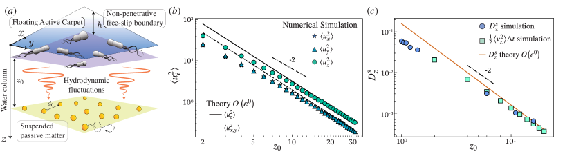
Figure 1: ($a$) An active carpet near the liquid-air interface generates flows that stir particles suspended below. ($b$) Strength of hydrodynamic fluctuations as a function of distance from the AC. Markers represent simulation results and lines represent the theoretical prediction from equation (3b). ($c$) Single-particle diffusivity in the $z$ direction. Circles are results from simulated MSDs, the squares are results from simulating the variance following equation (5), and the solid orange line represents the theoretical prediction from Eqs. (3b) and (5).

We consider the case where the induced flow is probed by passive tracers that are far from the free-slip surface, compared to the position of the swimmers. Therefore, we make the substitution $z_{s}=\varepsilon\,z$ with $\varepsilon\ll 1$, and perform a Taylor expansion on the flow exerted by a single swimmer, obtaining

$$\bm{u}\left(\bm{r},\bm{r}_{s},\bm{\hat{p}}_{s}\right)=\bm{u}_{(\varepsilon=0)}+\frac{\partial\bm{u}}{\partial\varepsilon}\bigr{\rvert}_{0}\varepsilon+\mathcal{O}\left(\varepsilon^{2}\right).$$

Evaluating the velocity field at $\bm{r}=(0,0,z)$, with $\bm{r}_{s}=(\rho_{s}\cos\theta_{s},\rho_{s}\sin\theta_{s},h)$ and $\bm{\hat{p}}=(\cos\phi_{s},\sin\phi_{s},0)$, the approximated far-field velocity field is,

$$(u_{x},u_{y})=\frac{\kappa\,\rho_{s}[2z^{2}-\rho_{s}^{2}(1+3\cos(2(\theta_{s}-\phi_{s})))]}{(z^{2}+\rho_{s}^{2})^{5/2}}(\cos\theta_{s},\sin\theta_{s}),$$ (2a)

$$u_{z}=\frac{z\kappa[-2z^{2}+\rho_{s}(1+3\cos(2(\theta_{s}-\phi_{s})))]}{(z^{2}+\rho_{s}^{2})^{5/2}}.$$ (2b)

We consider an AC with a uniform number density equal to $n$ organisms per unit area, and with uniformly distributed orientations, so the AC probability density function is $f(\bm{r}_{s},\bm{\hat{p}}_{s})=n/2\pi$. The ensemble-averaged flow field induced by an active carpet is $\langle\bm{u}\rangle=\int_{0}^{\infty}\int_{-\pi}^{\pi}\int_{-\pi}^{\pi}f\,\bm{u}(\bm{r},\bm{r}_{s},\hat{\bm{p}}_{s})\,{\rm d}\phi_{s}\,{\rm d}\theta_{s}\,\rho_{s}{\rm d}\rho_{s}=0.$ Thus, the mean flow at any instant is equal to zero for an infinite uniform AC, as expected by symmetry. However, the variances of the hydrodynamic fluctuations are not. We can derive them as follows:

$$\langle u_{i}u_{j}\rangle=\int_{0}^{\infty}\int_{-\pi}^{\pi}\int_{-\pi}^{\pi}\frac{n}{2\pi}\,u_{i}u_{j}\,{\rm d}\phi_{s}\,{\rm d}\theta_{s}\,\rho_{s}{\rm d}\rho_{s},$$ (3a)

$$\langle u_{x}^{2}\rangle=\langle u_{y}^{2}\rangle=\frac{9\pi n\kappa^{2}}{8z^{2}},\hskip 7.11317pt\langle u_{z}^{2}\rangle=\frac{11\pi n\kappa^{2}}{16z^{2}}.$$ (3b)

Thus, the intensity of the hydrodynamic fluctuations depends on the surface density of microswimmers, $n$. Moreover, they scale with the square of the individual flow strength, $\kappa^{2}$, so they are the same for puller-type and pusher-type swimmers. Finally, the fluctuations scale with the inverse of the distance squared, $1/z^{2}$, so they are stronger nearby and weaker further away from the AC.

To test our analytical theory, we also perform numerical simulations where the ACs are implemented explicitly as a large set of discrete, non-interacting point dipoles. They are randomly distributed across a horizontal square surface with a side length of $L=Nh$, where $N$ is a large integer ranging from $10^{3}$ to $10^{4}$. The surface density of microswimmers within the carpet is fixed to $n=0.1/h^{2}$, so the total number of organisms in the carpet is given by $N_{s}=nL^{2}=0.1N^{2}$. To evaluate the variances of the hydrodynamic fluctuations we computed in equation (3b), we compute the average $\langle\cdot\rangle$ over a large ensemble of independent AC configurations. In each AC configuration, the $N_{s}$ microswimmers are given new random positions and random orientations within the $x$-$y$ plane where the colony lives.

In what follows, time and length units are fixed such that $h=1$ and $\kappa=30$. We then consider $N_{t}$ tracer particles to gather statistics for the stochastic tracer dynamics. The equation of motion of the $\alpha$-th tracer is controlled by the flows induced by the AC:

$$\frac{{\rm d}\bm{r}_{\alpha}}{{\rm d}t}=\sum_{s}^{N_{s}}\bm{u}_{s}(\bm{r}_{\alpha},\bm{r}_{s},{\bm{\hat{p}})},$$ (4)

where $\bm{u}_{s}(\bm{r}_{\alpha},\bm{r}_{s},\bm{\hat{p}})$ is the velocity field produced by an individual microswimmer at a position $\bm{r}_{s}$ and orientation $\bm{\hat{p}}$, acting on a tracer placed at $\bm{r}_{\alpha}$, using either the full expression from equation (1) or the far field approximation from equation (2).

3 Results

3.1 Hydrodynamic fluctuations

We first focus on examining the velocity variance. Numerically, we produce a large ensemble of AC configurations and evaluate each variance component for a given initial tracer depth $z_{0}$. The simulation box has a size $L=10^{3}$, in which $N_{s}=10^{5}$ swimmers were placed. Figure 1$(b)$ compares the analytical solution for the variance found in equation (3b) (black and dashed lines) with full numerical simulations (markers). Notice that the parallel fluctuations, $\langle u_{x}^{2}\rangle$ and $\langle u_{y}^{2}\rangle$, are about 60% larger than the vertical fluctuations, $\langle u_{z}^{2}\rangle$, showing a significant anisotropic behaviour. The results show that the far-field theory is less accurate close to the AC, $z_{0}\lesssim 10$, but it offers a good approximation at long distances from the AC. These results clearly show that the hydrodynamic fluctuations are space-dependent in the vertical direction, decaying as $\langle u_{i}^{2}\rangle\propto 1/z_{0}^{2}$ through the fluid column.

Compared to a solid no-slip boundary, where $\langle u_{i}^{2}\rangle\propto 1/z_{0}^{4}$ (Guzmán-Lastra et al., 2021), these fluctuations near a liquid-air interface are much longer ranged, giving rise to a larger region of influence.

3.2 Single-particle diffusivity

Secondly, we examine the diffusion of particles that is caused by the hydrodynamic fluctuations generated by the AC. To explicitly obtain their diffusivity, we consider the single-particle mean-squared displacement (MSD), given by

$$\langle\Delta r_{i}\Delta r_{j}\rangle=\sum_{t^{\prime}=0}^{\tilde{n}\Delta t}\sum_{t^{\prime\prime}=0}^{\tilde{n}\Delta t}\Big{\langle}u_{i}(\bm{r}_{0},t^{\prime})u_{j}(\bm{r}_{0},t^{\prime\prime})\Big{\rangle}\Delta t^{\prime}\Delta t^{\prime\prime},$$

where $\tilde{n}$ is the total number of time steps in the simulations. We consider the case where the flow fields are uncorrelated between two consecutive time steps. Each time step corresponds to a different independent snapshot of the AC with microswimmers that have randomly sampled positions and orientations. Then we have the relation $\langle u_{i}(\bm{r}_{0},t^{\prime})u_{j}(\bm{r}_{0},t^{\prime\prime})\rangle=\langle u_{i}(\bm{r}_{0})u_{j}(\bm{r}_{0})\rangle\delta_{t^{\prime}t^{\prime\prime}}$, leading to the following expression for the MSD:

$$\langle\Delta r_{i}\Delta r_{j}\rangle=\langle u_{i}(\bm{r}_{0})u_{j}(\bm{r}_{0})\rangle\sum_{t^{\prime}=0}^{\tilde{n}\Delta t}\sum_{t^{\prime\prime}=0}^{\tilde{n}\Delta t}\delta_{t^{\prime}t^{\prime\prime}}\Delta t^{\prime}\Delta t^{\prime\prime}=\langle u_{i}u_{j}\rangle\tilde{n}\Delta t^{2}=\langle u_{i}u_{j}\rangle\Delta t\,t_{f},$$

where $t_{f}=\tilde{n}\Delta t$ denotes the final integration time. Therefore, we have $\langle\Delta r_{i}^{2}\rangle=\langle u_{i}^{2}\rangle\Delta t\,t_{f}\equiv 2D_{i}^{s}t_{f}$, so the single-particle diffusivity is

$$D_{i}^{s}\equiv\frac{1}{2}\langle u_{i}^{2}\rangle\Delta t.$$ (5)

To verify this numerically, we place tracers initially at $z_{0}$ and we compute their MSD for $\tilde{n}=10^{2}$ time steps. Figure 1(c) shows the single-particle diffusivity $D_{i}^{s}$ for $i=z$ as a function of $z_{0}$ obtained from the simulations and from the theory. The simulated observable $\langle u_{z}^{2}\rangle\Delta t/2$ is shown as green squares, and the diffusivity, $D_{z}^{s}$, obtained from the simulated MSDs, is displayed as blue circles. These markers collapse onto a single curve, which is compared with the theory from equation (5) shown by the orange line. Indeed, the results exhibit strong agreement between theory and simulations. As predicted, the diffusivity decays with an exponent of $-2$ for large $z_{0}$. This implies that particle stirring significantly intensifies near the AC, potentially enhancing particle encounters, which we consider next.

3.3 Velocity pair correlation

Thirdly, we look at how pairs of suspended particles respond to fluid distortions caused by the AC. Although the generated flow is time-uncorrelated, the spatial structure is more complex: Particles that are initially located close to each other follow adjacent streamlines that are almost parallel to each other, so their motions remain correlated at short distances. By contrast, with larger initial separations, the particles will follow different streamlines and separate further from each other. This relative motion is quantified by the velocity pair correlation function,

$$g_{p}(d_{0},z_{0})=\frac{\langle u_{x}(\bm{r}_{1})u_{x}(\bm{r}_{2})\rangle}{\sqrt{\langle u_{x}^{2}(\bm{r}_{1})\rangle\langle u_{x}^{2}(\bm{r}_{2})\rangle}},$$ (6)

where the initial positions of the two particles are $\bm{r}_{1}=(d_{0}/2\sqrt{2},d_{0}/2\sqrt{2},z_{0})$ and $\bm{r}_{2}=(-d_{0}/2\sqrt{2},-d_{0}/2\sqrt{2},z_{0})$, which are located at the same distance from the carpet $z_{0}$ and separated laterally by $d_{0}$. Notice that the velocity pair correlation is symmetric in the $x$ and $y$ directions.

Numerically, we sample over $10^{4}$ ensembles, each with $N_{s}=10^{7}$ swimmers, to measure the velocity using equation (1) at the positions $\bm{r}_{1}$ and $\bm{r}_{2}$ given above, with $z_{0}$ in the range $[2,20]$ and $d_{0}$ in the range [$10^{-3}$, $10^{3}$]. The resulting velocity pair correlations are shown as circles in figure 2(a). As predicted, we find that pairs become progressively more uncorrelated with distance $d_{0}$. Moreover, the separation required for the pairs to become uncorrelated grows with $z_{0}$. Notably, when the velocity pair correlations are plotted in terms of the scaled distance $d_{0}/z_{0}$, there is a collapse for all depths onto a single curve, as shown in the inset of figure 2(a). Globally, velocities decorrelate at distances larger than $d_{0}\gtrsim 7z_{0}$. This result already suggests that as we move away from the AC, only large particles may collide. We will examine that in more detail later. First, we propose a heuristic model for the collapsed velocity correlation of the form

$$g_{p}^{\text{model}}(\xi)=\exp(-\xi)[A_{1}\sin(\xi)+\cos(\xi)]+\exp(-\xi/A_{2})[A_{3}+A_{4}\xi],$$ (7)

where $\xi=d_{0}/z_{0}$. Using least squares to fit this model to our simulation data, we find that the optimal fitting parameters are $A_{1}=0.097$, $A_{2}=1.3$, $A_{3}=-0.014$, $A_{4}=0.89$. The resulting model is shown as coloured lines for the different $z_{0}$ values in figure 2(a), and also in the inset.

Analytical progress can be made by using the far-field approximation, where $g_{p}$ can be obtained by evaluating the velocity from equation (2) and the variances from equation (3) at the positions $\bm{r}_{1}$ and $\bm{r}_{2}$, which gives

$$g_{p}(d_{0},z_{0})=\frac{1}{\langle u_{x}^{2}\rangle}\int_{0}^{2\pi}\int_{0}^{2\pi}\int_{0}^{\infty}u_{x}(\bm{r}_{1})u_{x}(\bm{r}_{2})\frac{n}{2\pi}\rho_{s}{\rm d}\rho_{s}{\rm d}\theta_{s}{\rm d}\phi_{s}.$$ (8)

It is challenging to find a closed-form expression for this integral, but it can be evaluated numerically. This semi-analytical result is shown in the inset of figure 2$(a)$. This theory result agrees well with our simulations and highlights the importance of the vertical distance to the AC: It does not only determine the strength of the hydrodynamic fluctuations, but also the relative motion of the flow structures. Particles at greater depths tend to move together more, which directly impacts their pair diffusivity, as we will see next.

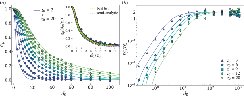
Figure 2: (a) Velocity pair correlation as a function of horizontal particle separation. Coloured circles represent simulation results for different depths, ranging from $z_{0}=2$ (blue) to $z_{0}=20$ (light green), each separated by $\Delta z_{0}=2$. Lines represent the best fit to the model from equation  (7). Inset: These curves collapse when plotted as $d_{0}/z_{0}$. The yellow line is the best fit from equation  (7), and the pink dashed line is the semi-analytical result obtained by numerically integrating $g_{p}(d_{0},z_{0})$. (b) Pair diffusivity as a function of horizontal particle separation, normalised by the single-particle diffusivity. Markers represent simulation values for different depths, $z_{0}$. The black dashed line is the theoretical asymptotic value from $D_{i}^{p\infty}$.

3.4 Pair diffusion

We now explore how an AC drives can mix two particles up, as a function of their distance. This is quantified by the ‘pair diffusivity’. Numerically, we sample the carpet as described previously. Two tracers are put initially at the positions $\bm{r}_{1}$ and $\bm{r}_{2}$, after which they follow the equation of motion, equation  (4). The integration time step is $\Delta t=10^{-3}$. Averages are performed over $300$ pair trajectories. The pair diffusivity $D_{\rho}^{p}$ in the $xy$ plane is obtained by measuring the pair’s distance squared, $\Delta\rho^{2}(t)=\left(|\bm{r}_{1}(t)-\bm{r}_{2}(t)|-d_{0}\right)^{2}$. After the simulation ends, each $\Delta\rho^{2}$ curve is fitted with a power-law function of the form $4D_{\rho}^{p}\,t^{b}$. Results show that all curves follow a diffusive regime ($b\sim 1$).

Figure 2(b) displays the resulting pair diffusivity $D_{\rho}^{p}$, normalised by the single-particle diffusivity $D^{s}_{p}$, as a function of the initial horizontal particle separation $d_{0}$. For small separations, the particles follow almost the same streamlines, so their relative motion and pair diffusivity is small. Indeed, it is difficult to mix particles that are close to each other, as we observe in the kitchen when stirring macaron batter (Mathijssen et al., 2023). At large particle separations, it gets easier to mix them, so the pair diffusivity increases with $d_{0}$ until it plateaus.

To predict this analytically, we define $\bm{r}_{12}=\bm{r}_{1}-\bm{r}_{2}$. Similar to the single-particle MSD calculation, the pair MSD is then computed as follows,

$$\langle\Delta r_{12i}\Delta r_{12j}\rangle=\langle\Delta r_{1i}\Delta r_{1j}\rangle+\langle\Delta r_{2i}\Delta r_{2j}\rangle-\langle\Delta r_{1i}\Delta r_{2j}\rangle-\langle\Delta r_{2i}\Delta r_{1j}\rangle,$$ (9)

where $\Delta r_{\alpha i}$ denotes the displacement of the particle $\alpha$ along coordinate $i$ and analogously for $\Delta r_{12i}$. On average, terms 1 and 2 on the RHS of equation  (9) are the same, and terms 3 and 4 are also equal to each other. Therefore, $\langle\Delta r_{12i}\Delta r_{12j}\rangle=2\langle\Delta r_{1i}\Delta r_{1j}\rangle-2\langle\Delta r_{1i}\Delta r_{2j}\rangle$. Considering $i=j$, the first term is $\langle\Delta r_{i}\Delta r_{i}\rangle=2D_{i}^{s}t$, with $D_{i}^{s}$ the single diffusivity in the $i$-coordinate. The second term can be estimated in a similar way as in the single MSD calculation, $\langle\Delta r_{1i}\Delta r_{2i}\rangle=\sum_{t^{\prime}=0}^{\tilde{n}\Delta t}\sum_{t^{\prime\prime}=0}^{\tilde{n}\Delta t}\langle u_{1i}u_{2i}\rangle\Delta t^{\prime}\Delta t^{\prime\prime}$. The function to be integrated is the complete spatiotemporal pair correlation velocity, $\langle u_{1i}u_{2i}\rangle(d_{0},z_{0},t)=\langle u_{i}^{2}\rangle g_{p}(d_{0},z_{0})\delta_{t^{\prime}t^{\prime\prime}}$ where $g_{p}$ is the spatial pair velocity correlation defined in 6. With this, we obtain $\langle\Delta r_{1i}\Delta r_{2i}\rangle=\langle u_{i}^{2}\rangle g_{p}\sum_{t^{\prime}=0}^{\tilde{n}\Delta t}\sum_{t^{\prime\prime}=0}^{\tilde{n}\Delta t}\delta_{t^{\prime}t^{\prime\prime}}\Delta t^{\prime}\Delta t^{\prime\prime}=\langle u_{i}^{2}\rangle g_{p}\Delta t\,t_{f}$. Thus, $\langle(\Delta r_{12i})(\Delta r_{12j})\rangle=2\left(2D_{i}^{s}-\langle u_{i}^{2}\rangle\Delta tg_{p}\right)t_{f}$, where we obtain the pair diffusivity

$$D_{i}^{p}\equiv 2D_{i}^{s}-\langle u_{i}^{2}\rangle\Delta tg_{p}=2D_{i}^{s}(1-g_{p}).$$ (10)

This expression depends upon the variance and single diffusivity relation in equation  (5). Since the function $g_{p}(d_{0},z_{0})$ decays exponentially with the distance $d_{0}$, the asymptotic pair diffusivity is readily predicted for large $d_{0}$,

$$\lim_{d_{0}\to\infty}D_{i}^{p}\equiv D_{i}^{p\infty}=2D_{i}^{s}.$$ (11)

Figure 2(b) shows this theoretical result for the pair diffusivity from equation  (10), using $g^{\text{model}}_{p}$ from equation  (7). This result agrees well with the simulations, as shown for various distances $z_{0}$.

Interestingly, the observed diffusive behaviour in our study bears a resemblance to turbulent systems, as seen in (Belan & Kardar, 2019), where a pair of tracers within a 3D bath of microswimmers also exhibited an asymptotic diffusivity twice that of their self-diffusion. Our results reveal that the distance parameter $z_{0}$ significantly affects diffusivity. The mixing becomes more intense and converges to the asymptotic value when particles are closer to the AC. This phenomenon can be attributed to amplified hydrodynamic fluctuations near the carpet, which disrupt spatial correlations in fluid flows. The parameter $d_{0}$ is also crucial; closer particles exhibit lower diffusion from each other compared to those at greater distances, resulting in synchronised movement and more similar trajectories. Consequently, the pair diffusivity might offer fundamental insights into aggregation phenomena, which we study next.

3.5 Particle aggregation

Last, we investigate whether fluctuations caused by ACs can initiate the aggregation of spherical particles of finite radius $a$. To model this, we consider a short-ranged pairwise sticky force between the particles. We consider the Morse model, given by $\bm{F}_{M}(\bm{r})=2UW\left[1-e^{-W(r-r_{\text{eq}})}\right]e^{-W(r-r_{\text{eq}})}\hat{\bm{r}}$, where $r=|\bm{r}|$ is the distance between the tracers. Here, $r_{\text{eq}}$ is the pair equilibrium distance, while $U$ and $W$ denote the depth and width of the potential well, respectively. The force is scaled with the Stokes mobility, so it has units of velocity. By setting $r_{\text{eq}}$ to twice the radius $a$, $U$ to $10^{-9}$, and $W$ to 30, we position the potential minima along $r$, allowing for the precise adjustment of equilibrium distances for tracers with different radii $a$.

Initially, at $t=0$, the particles are placed in a square lattice of $N_{t}=19\times 19=361$ particles located at the same depth $z_{0}$. The distance between their centers is equal to $d_{0}=\tilde{d}_{0}+2a$, where $\tilde{d}_{0}$ is the border-to-border distance between the particles. We always set $\tilde{d}_{0}=0.8$ and vary $d_{0}$ or equivalently $a$. Subsequently, for $t>0$, the particles start moving in the $x$-$y$ plane at a fixed depth $z_{0}$, following the equation of motion equation  (4) with the addition of the inter-particle sticking forces. Hence, they start colliding and aggregating to each other.

We then simulate the histogram of first passage times, defined as the time taken for particles to collide. These results are shown in the inset of figure 3(a). The red dashed line shows the mean first passage time, $\tau_{FP}$. This observable can also be estimated analytically by equating the pair MSD from equation  (10) to the border-to-border distance between particles, $\tilde{d_{0}}^{2}\approx\langle\Delta r_{1}\Delta r_{2}\rangle=4D_{p}^{\rho}\tau_{\text{FP}}$, so the mean first passage time is

$$\tau_{\text{FP}}\approx\frac{\tilde{d_{0}}^{2}}{4D_{p}^{\rho}}.$$ (12)

This theoretical prediction for $\tau_{FP}$ agrees well with the numerical simulations, as shown for $z_{0}=3$ by the solid green line in figure 3($a$). This provides a reliable estimate for the average collision time between two particles due to the hydrodynamic stirring induced by the AC.

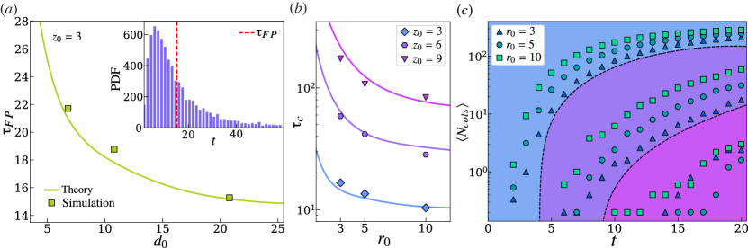
Figure 3: ($a$) Mean first passage time of particle collisions as a function of the horizontal particle separation, $d_{0}$, for particles initially located at $z_{0}=3$. Squares represent simulations and the line is the prediction $\tau_{\text{FP}}\approx\tilde{d_{0}}^{2}/4D_{p}^{\rho}.$ Insite: Histogram of first passage times. The vertical red dashed line is the mean first passage time. ($b$) Clearance time against particle radius for three depths. Symbols show simulation results, and solid lines show $\tau_{c}\sim 0.7\tau_{FP}$. ($c$) Average accumulated number of collisions over time. Markers show averaged simulation results for different particle radii, ranging from $a=3$ (triangles) to $a=10$ (squares). The background colours represent different depths, ranging from $z_{0}=3$ (light blue) to $z_{0}=9$ (pink).

In addition, we calculate the average ‘clearance time’ denoted as $\tau_{c}$. This is the time taken for half of the particles in the suspension to have collided. This observable represents a fundamental time scale of particle aggregation (Font-Muñoz et al., 2019; Wang et al., 1998). The graph shown in figure 3(b) illustrates the clearance time, where we assume that particles stick together after a collision. Therefore, $\tau_{c}$ is a crucial indicator for cluster formation. Our results show that, as the size of the particle $a$ increases, the clearance time decreases. Moreover, $\tau_{FP}$ and $\tau_{c}$ are proportional to each other since they both arise from the same physical process. Empirically, we observe that $\tau_{c}\sim 0.7\tau_{\text{FP}}$ for every $z_{0}$, as shown by the lines in figure 3(b), which agree well with the simulations.

Last, we measured the time evolution of the average accumulated number of collisions $\langle N_{cols}\rangle$ for this configuration. Figure 3$(c)$ shows $\langle N_{cols}\rangle$ over time for each $z_{0}$. We observe a close correlation between $\langle N_{cols}\rangle$ and $\tau_{c}$, as expected. Collisions become more frequent as we move closer to the AC and increase with larger particle radii. This suggests that the pair correlation function $g_{p}$ in equation  (6) governs both the collisions and the measured aggregation times. As the particle size increases, the correlation among their centres decreases, making it easier for them to follow different trajectories and ultimately leading to more collisions. In contrast, the intense fluctuations near ACs disrupt this correlation, increasing the likelihood of collisions.

4 Concluding remarks

Here, we have established analytical connections between the flows generated by active carpets and the aggregation dynamics of suspended particles. Our key findings include: (i) An analytical solution for hydrodynamic fluctuations produced by active carpets near fluid-air interfaces; (ii) the emergence of space-dependent and anisotropic diffusion, which decreases quadratically with distance; (iii) the role of hydrodynamic fluctuations in facilitating pairing encounters, where particle aggregation is favoured for large compared to small particles; (iv) the mean first-passage time between collisions decreases as particles move farther apart; (v) in the close vicinity of active carpets, intense hydrodynamic stirring accelerates clearance times and particle aggregation processes. This research highlights the pivotal role of biologically driven flows in the transport and spatial organisation of particles in aquatic systems, while serving as a noteworthy example of an out-of-equilibrium system that remains analytically tractable.

Acknowledgments. The authors are grateful for the helpful feedback given Hartmut Löwen and Felipe Barros.

Fundings. G.A., R.S. and F.G.-L. have received support from the ANID – Millennium Science Initiative Program – NCN19 170, Chile. F.G.-L. was supported by Fondecyt Iniciación No. 11220683. H.N.U. and A.J.T.M.M. were supported by start-up grants from the University of Pennsylvania. A.J.T.M.M. acknowledges funding from the United States Department of Agriculture (USDA-NIFA AFRI grants 2020-67017-30776 and 2020-67015-32330), the Charles E. Kaufman Foundation (Early Investigator Research Award KA2022-129523) and the University of Pennsylvania (University Research Foundation Grant and Klein Family Social Justice Award).

Declaration of interests. The authors report no conflict of interest.

Author ORCIDs

Gabriel Aguayo    https://orcid.org/0009-0004-4915-2707
Arnold Mathijssen    https://orcid.org/0000-0002-9577-8928
Hugo N. Ulloa    https://orcid.org/0000-0002-1995-6630
Rodrigo Soto   https://orcid.org/0000-0003-1315-5872
Francisca Guzman-Lastra    https://orcid.org/0000-0002-1906-9222

References

- Ahmadzadegan et al. (2019) Ahmadzadegan, A., Wang, S., Vlachos, P. P. & Ardekani, A. M. 2019 Hydrodynamic attraction of bacteria to gas and liquid interfaces. Phys. Rev. E 100 (6), 062605.
- Alert et al. (2022) Alert, R., Casademunt, J. & Joanny, J.-F.çois 2022 Active turbulence. Annu. Rev. Condens. Matter Phys. 13, 143–170.
- Angelani et al. (2011) Angelani, L., Maggi, C., Bernardini, M.L., Rizzo, A. & Di Leonardo, R. 2011 Effective interactions between colloidal particles suspended in a bath of swimming cells. Phys. Rev. Lett. 107 (13), 138302.
- Arguedas-Leiva et al. (2022) Arguedas-Leiva, J.-A., Słomka, J., Lalescu, C. C., Stocker, R. & Wilczek, M. 2022 Elongation enhances encounter rates between phytoplankton in turbulence. Proc. Natl. Acad. Sci. 119 (32), e2203191119.
- Belan & Kardar (2019) Belan, S. & Kardar, M. 2019 Pair dispersion in dilute suspension of active swimmers. J. Chem. Phys. 150 (6), 064907.
- Berke et al. (2008) Berke, A. P, Turner, L., Berg, H. C. & Lauga, E. 2008 Hydrodynamic attraction of swimming microorganisms by surfaces. Phys. Rev. Lett. 101 (3), 038102.
- Burd & Jackson (2009) Burd, Adrian B & Jackson, George A 2009 Particle aggregation. Annual Review of Marine Science 1, 65–90.
- Camassa et al. (2019) Camassa, Roberto, Harris, Daniel M, Hunt, Robert, Kilic, Zeliha & McLaughlin, Richard M 2019 A first-principle mechanism for particulate aggregation and self-assembly in stratified fluids. Nature Communications 10 (1), 5804.
- Cruz & Neuer (2022) Cruz, Bianca N & Neuer, Susanne 2022 Particle-associated bacteria differentially influence the aggregation of the marine diatom minutocellus polymorphus. ISME Communications 2 (1), 73.
- Dabiri (2010) Dabiri, John O 2010 Role of vertical migration in biogenic ocean mixing. Geophys. Res. Lett. 37 (11).
- Dani et al. (2022) Dani, A., Yeganeh, M. & Maldarelli, C. 2022 Hydrodynamic interactions between charged and uncharged brownian colloids at a fluid-fluid interface. Journal of Colloid and Interface Science 628, 931–945.
- Desai & Ardekani (2020) Desai, Nikhil & Ardekani, Arezoo M 2020 Biofilms at interfaces: microbial distribution in floating films. Soft Matter 16 (7), 1731–1750.
- Drescher et al. (2011) Drescher, K., Dunkel, J., Cisneros, L. H., Ganguly, S. & Goldstein, R. E. 2011 Fluid dynamics and noise in bacterial cell–cell and cell–surface scattering. Proceedings of the National Academy of Sciences 108 (27), 10940–10945.
- Durham & Stocker (2012) Durham, W. M. & Stocker, R. 2012 Thin phytoplankton layers: characteristics, mechanisms, and consequences. Annual Review of Marine Science 4, 177–207.
- Font-Muñoz et al. (2019) Font-Muñoz, J. S., Jeanneret, R., Arrieta, J., Anglès, S., Jordi, A., Tuval, I. & Basterretxea, G. 2019 Collective sinking promotes selective cell pairing in planktonic pennate diatoms. Proceedings of the National Academy of Sciences 116 (32), 15997–16002.
- Gokhale et al. (2022) Gokhale, Shreyas, Li, Junang, Solon, Alexandre, Gore, Jeff & Fakhri, Nikta 2022 Dynamic clustering of passive colloids in dense suspensions of motile bacteria. Physical Review E 105 (5), 054605.
- Gonzalez et al. (2021) Gonzalez, E., Aponte-Rivera, C. & Zia, R. N. 2021 Impact of polydispersity and confinement on diffusion in hydrodynamically interacting colloidal suspensions. J. Fluid Mech. 925, A35.
- de Graaf & Stenhammar (2017) de Graaf, Joost & Stenhammar, Joakim 2017 Stirring by periodic arrays of microswimmers. J. Fluid Mech. 811, 487–498.
- Guzmán-Lastra et al. (2021) Guzmán-Lastra, F., Löwen, H. & Mathijssen, A. JTM 2021 Active carpets drive non-equilibrium diffusion and enhanced molecular fluxes. Nature Communications 12 (1), 1906.
- Hamada et al. (2020) Hamada, Mayumi, Cueto-Felgueroso, Luis & de Anna, Pietro 2020 Diffusion limited mixing in confined media. Phys. Rev. Fluids 5 (12), 124502.
- Happel & Brenner (1983) Happel, J. & Brenner, H. 1983 Low Reynolds number hydrodynamics: with special applications to particulate media, , vol. 1. Springer Science & Business Media.
- Hill & Pedley (2005) Hill, NA & Pedley, TJ 2005 Bioconvection. Fluid Dynamics Research 37 (1-2), 1.
- Javadi et al. (2020) Javadi, Armand, Arrieta, Jorge, Tuval, Idan & Polin, Marco 2020 Photo-bioconvection: towards light control of flows in active suspensions. Philosophical Transactions of the Royal Society A 378 (2179), 20190523.
- Jeanneret et al. (2016) Jeanneret, Raphaël, Pushkin, Dmitri O, Kantsler, Vasily & Polin, Marco 2016 Entrainment dominates the interaction of microalgae with micron-sized objects. Nature communications 7 (1), 12518.
- Jia et al. (2019) Jia, Yankai, Huang, Renjing, Lan, Yang, Ren, Yukun, Jiang, Hongyuan & Lee, Daeyeon 2019 Reversible aggregation and dispersion of particles at a liquid–liquid interface using space charge injection. Advanced Materials Interfaces 6 (5), 1801920.
- Jin et al. (2021) Jin, Chenyu, Chen, Yibo, Maass, Corinna C & Mathijssen, Arnold JTM 2021 Collective entrainment and confinement amplify transport by schooling microswimmers. Phys. Rev. Lett. 127 (8), 088006.
- Kanale et al. (2022) Kanale, Anup V, Ling, Feng, Guo, Hanliang, Fürthauer, Sebastian & Kanso, Eva 2022 Spontaneous phase coordination and fluid pumping in model ciliary carpets. Proceedings of the National Academy of Sciences 119 (45), e2214413119.
- Kushwaha et al. (2023) Kushwaha, P., Semwal, V., Maity, S., Mishra, S. & Chikkadi, V. 2023 Phase separation of passive particles in active liquids. Physical Review E 108 (3), 034603.
- Lambert et al. (2013) Lambert, Ruth A, Picano, Francesco, Breugem, Wim-Paul & Brandt, Luca 2013 Active suspensions in thin films: nutrient uptake and swimmer motion. J. Fluid Mech. 733, 528–557.
- Lauga (2020) Lauga, E. 2020 The fluid dynamics of cell motility, , vol. 62. Cambridge University Press.
- Loi et al. (2008) Loi, Davide, Mossa, Stefano & Cugliandolo, Leticia F 2008 Effective temperature of active matter. Phys. Rev. E 77 (5), 051111.
- Madden et al. (2022) Madden, I. P., Wang, L., Simmchen, J. & Luijten, E. 2022 Hydrodynamically controlled self-organization in mixtures of active and passive colloids. Small 18 (21), 2107023.
- Maheshwari et al. (2019) Maheshwari, Akshay J, Sunol, Alp M, Gonzalez, Emma, Endy, Drew & Zia, Roseanna N 2019 Colloidal hydrodynamics of biological cells: A frontier spanning two fields. Phys. Rev. Fluids 4 (11), 110506.
- Mathijssen et al. (2016) Mathijssen, Arnold JTM, Doostmohammadi, Amin, Yeomans, Julia M & Shendruk, Tyler N 2016 Hydrodynamics of micro-swimmers in films. J. Fluid Mech. 806, 35–70.
- Mathijssen et al. (2018a) Mathijssen, A. JTM, Guzmán-Lastra, F., Kaiser, A. & Löwen, H. 2018a Nutrient transport driven by microbial active carpets. Phys. Rev. Lett. 121 (24), 248101.
- Mathijssen et al. (2018b) Mathijssen, Arnold JTM, Jeanneret, Raphaël & Polin, Marco 2018b Universal entrainment mechanism controls contact times with motile cells. Phys. Rev. Fluids 3 (3), 033103.
- Mathijssen et al. (2023) Mathijssen, Arnold J. T. M., Lisicki, Maciej, Prakash, Vivek N. & Mossige, Endre J. L. 2023 Culinary fluid mechanics and other currents in food science. Reviews of Modern Physics 95, 025004.
- Mino et al. (2011) Mino, Gastón, Mallouk, Thomas E, Darnige, Thierry, Hoyos, Mauricio, Dauchet, Jeremi, Dunstan, Jocelyn, Soto, Rodrigo, Wang, Yang, Rousselet, Annie & Clement, Eric 2011 Enhanced diffusion due to active swimmers at a solid surface. Phys. Rev. Lett. 106 (4), 048102.
- Miño et al. (2013) Miño, G. L., Dunstan, J., Rousselet, A., Clément, E. & Soto, Rodrigo 2013 Induced diffusion of tracers in a bacterial suspension: theory and experiments. J. Fluid Mech. 729, 423–444.
- Morozov & Marenduzzo (2014) Morozov, Alexander & Marenduzzo, Davide 2014 Enhanced diffusion of tracer particles in dilute bacterial suspensions. Soft Matter 10 (16), 2748–2758.
- Omar et al. (2018) Omar, A. K., Wu, Y., Wang, Z.-G. & Brady, J. F. 2018 Swimming to stability: structural and dynamical control via active doping. ACS nano 13 (1), 560–572.
- Ortlieb et al. (2019) Ortlieb, Levke, Rafaï, Salima, Peyla, Philippe, Wagner, Christian & John, Thomas 2019 Statistics of colloidal suspensions stirred by microswimmers. Phys. Rev. Lett. 122 (14), 148101.
- Pedley & Kessler (1992) Pedley, TJ & Kessler, JO 1992 Bioconvection. Science Progress (1933-) pp. 105–123.
- Pellicciotta et al. (2020) Pellicciotta, Nicola, Hamilton, Evelyn, Kotar, Jurij, Faucourt, Marion, Delgehyr, Nathalie, Spassky, Nathalie & Cicuta, Pietro 2020 Entrainment of mammalian motile cilia in the brain with hydrodynamic forces. Proceedings of the National Academy of Sciences 117 (15), 8315–8325.
- Pushkin & Yeomans (2013) Pushkin, Dmitri O & Yeomans, Julia M 2013 Fluid mixing by curved trajectories of microswimmers. Phys. Rev. Lett. 111 (18), 188101.
- Sengupta et al. (2017) Sengupta, Anupam, Carrara, Francesco & Stocker, Roman 2017 Phytoplankton can actively diversify their migration strategy in response to turbulent cues. Nature 543 (7646), 555–558.
- Simoncelli et al. (2017) Simoncelli, Stefano, Thackeray, Stephen J & Wain, Danielle J 2017 Can small zooplankton mix lakes? Limnology and Oceanography Letters 2 (5), 167–176.
- Sommer et al. (2017) Sommer, Tobias, Danza, Francesco, Berg, Jasmine, Sengupta, Anupam, Constantinescu, George, Tokyay, Talia, Bürgmann, Helmut, Dressler, Y, Sepúlveda Steiner, O, Schubert, CJ & others 2017 Bacteria-induced mixing in natural waters. Geophys. Res. Lett. 44 (18), 9424–9432.
- Takatori & Brady (2015) Takatori, Sho C & Brady, John F 2015 Towards a thermodynamics of active matter. Phys. Rev. E 91 (3), 032117.
- Vaccari et al. (2017) Vaccari, Liana, Molaei, Mehdi, Niepa, Tagbo HR, Lee, Daeyeon, Leheny, Robert L & Stebe, Kathleen J 2017 Films of bacteria at interfaces. Advances in colloid and interface science 247, 561–572.
- Wang et al. (1998) Wang, Lian-Ping, Wexler, Anthony S & Zhou, Yong 1998 On the collision rate of small particles in isotropic turbulence. i. zero-inertia case. Physics of Fluids 10 (1), 266–276.
- Wang & Ardekani (2015) Wang, Shiyan & Ardekani, Arezoo M 2015 Biogenic mixing induced by intermediate reynolds number swimming in stratified fluids. Scientific Reports 5 (1), 17448.
- Zhan et al. (2014) Zhan, Caijuan, Sardina, Gaetano, Lushi, Enkeleida & Brandt, Luca 2014 Accumulation of motile elongated micro-organisms in turbulence. J. Fluid Mech. 739, 22–36.