Jet Classification Using High-Level Features from Anatomy of Top Jets

Abstract

Recent advancements in deep learning models have significantly enhanced jet classification performance by analyzing low-level features (LLFs). However, this approach often leads to less interpretable models, emphasizing the need to understand the decision-making process and to identify the high-level features (HLFs) crucial for explaining jet classification. To address this, we introduce an analysis model (AM) that analyzes selected HLFs designed to capture important features of top jets. Our AM mainly consists of the following three modules: a relation network analyzing two-point energy correlations, mathematical morphology and Minkowski functionals for generalizing jet constituent multiplicities, and a recursive neural network analyzing subjet constituent multiplicity to enhance sensitivity to subjet color charges. We demonstrate that our AM achieves performance comparable to the Particle Transformer (ParT) in top jet tagging and simulated jet comparison at the hadronic calorimeter angular resolution scale while requiring fewer computational resources. Furthermore, as a more constrained architecture than ParT, the AM exhibits smaller training uncertainties because of the bias-variance tradeoff. We also compare the information content of AM and ParT by decorrelating the features already learned by AM.

1 Introduction

Understanding how to identify the initiating particle of jets in hadron collisions has been a crucial challenge in pursuing physics beyond the Standard Model. This problem becomes increasingly important as the Large Hadron Collider (LHC) accumulates substantial events for discovering new physics signatures at energies above the electroweak scale. The search involves the identification of the boosted heavy particles, such as $W/Z$ bosons, Higgs bosons, and top quarks, produced in hard processes with high energies. Those boosted particles often create collimated clusters similar to the jets originating from light quarks and gluons (QCD jets). Therefore, designing and understanding taggers separating the heavy particle-initiated jets from the QCD jets has been a crucial problem of collider physics, essential for maximizing the discovery potential of the LHC and future colliders.

Modern methods for jet tagging are based on deep learning algorithms to maximize the utilization of information in a jet. Deep learning classifiers are based on artificial neural networks capable of handling high-dimensional data and correlation among them. The flexibility and capability allow us to build a tagger directly analyzing low-level features (LLFs) like jet constituents. The early studies have concentrated on network architectures that analyze jets in representations close to those popular in computer science, such as jet images Cogan:2014oua ; Almeida:2015jua ; deOliveira:2015xxd ; Komiske:2016rsd ; Kasieczka:2017nvn ; Macaluso:2018tck ; Farina:2018fyg ; Lin:2018cin and clustering sequences Guest:2016iqz ; Louppe:2017ipp ; Cheng:2017rdo . These deep learning-based classifiers have significantly outperformed traditional methods, which rely on a limited number of high-level features (HLFs) designed to capture specific substructural features of heavy particle-initiated jets Butterworth:2008iy ; Kaplan:2008ie ; Plehn:2010st ; Plehn:2011sj ; Thaler:2010tr ; Thaler:2011gf ; Larkoski:2013eya ; Larkoski:2014gra by orders of magnitude. Consequently, deep learning has been regarded as a promising approach for boosting the sensitivity of the LHC experiments in detecting new physics.

The state-of-the-art (SoTA) models in classification performances are based on graph neural networks graphnn and transformers NIPS2017_3f5ee243 . First examples in jet physics include ParticleNet Qu:2019gqs based on dynamic graph convolutional neural networks 10.1145/3326362 and Particle Flow Network Komiske:2018cqr based on deep sets NIPS2017_f22e4747 . ParticleNet outperformed image-based approaches in top jet tagging Kasieczka:2019dbj and has gained significant attention CMS-PAS-BTV-22-001 . Graph neural networks are also convenient in fusing physics constraints, such as imposing IRC-safety in terms of energy correlators NIPS2017_f22e4747 ; Chakraborty:2020yfc , using symmetry equivariant layers Gong:2022lye ; Bogatskiy:2022czk and using Lund plane Dreyer:2018nbf ; Dreyer:2020brq inspired correlations between jet constituents Qu:2022mxj . The most advanced taggers currently are graph neural networks that incorporate physics knowledge: Particle Transformer Qu:2022mxj , LorentzNet Gong:2022lye , and PELICAN Bogatskiy:2022czk , as the additional constraint simplifies the problem while preserving networks’ capabilities.

Deep learning-based taggers have shown impressive performance in learning all the detailed patterns of given jets; however, there are concerns about systematic uncertainties, particularly regarding the learning of features from soft QCD. Since the dynamics of the strong interaction at low energies are not perturbatively described, simulations rely on phenomenological models tuned to experimental data instead Buckley:2011ms ; Bierlich:2022pfr ; Bellm:2015jjp ; Sherpa:2019gpd . Consequently, the soft features in simulated jets can vary significantly from one simulation to another. This systematic variance poses a challenge in building taggers, especially the supervised classifiers trained on simulated jets, as they may become sensitive to the choice of simulation setups Barnard:2016qma ; Chakraborty:2019imr ; Chakraborty:2020yfc ; Lim:2020igi ; Dreyer:2020brq ; Ghosh:2021hrh , though in some cases, the simulation dependencies are minor Cheung:2022dil . A thorough understanding of the physics information utilized by each tagger is crucial to assess and minimize the systematic uncertainties and simulation bias of taggers.

To address this problem of understanding deep learning-based jet taggers, we revisit the classifiers based on HLFs. Compared to classifiers analyzing LLFs, taggers focusing on HLFs are more constrained and offer clearer interpretations in terms of physics. These characteristics make HLF-based taggers more interpretable, particularly when analyzing how HLFs influence network predictions Komiske:2017aww ; Komiske:2018cqr ; Chakraborty:2019imr . Additionally, constrained taggers typically exhibit smaller training uncertainties, such as variation in network predictions due to random initialization of networks or train/validation dataset splitting Chakraborty:2020yfc ; Das:2022cjl . This phenomenon is known as the bias-variance tradeoff, which suggests that constrained models tend to have less variance than more general models at the cost of performance.

What if HLF-based taggers are competitive with more general taggers such as graph neural networks? There would be two immediate advantages: network predictions would have less training uncertainty, and simpler taggers would require fewer computational resources. In principle, if we could design a set of HLFs that fully capture features crucial for jet tagging, we could develop a high-performing jet tagger based on HLFs. Additionally, such taggers could be further utilized for calibrating simulations when they are trained to distinguish simulations from the experimental data with high precision.

This paper is structured as follows to address the challenges discussed above. Section 2 introduces our analysis model, which consists of modules analyzing groups of HLFs that capture specific characteristic features of top jets. This model is an extension of our previous works Lim:2018toa ; Chakraborty:2019imr ; Chakraborty:2020yfc ; Lim:2020igi . Specifically, we will revisit a set of constituent multiplicities sensitive to subjet color charges, which are also important features in top jet tagging. We will introduce a recursive neural network analyzing these numbers to our framework.

In Section 3, we compare the performance of the analysis model to one of the state-of-the-art jet taggers, Particle Transformer (ParT) Qu:2022mxj . As a benchmark, we focus on top jet classification problems using various simulations, including Pythia Bierlich:2022pfr , Herwig Bellm:2015jjp , and Vincia Ritzmann:2012ca ; Fischer:2016vfv . Additionally, we compare jets simulated by different generators to assess each network’s ability to differentiate simulations. For simplicity, our discussion will concentrate on features at the angular scale above the hadronic calorimeter scale, 0.1. We will demonstrate that our model has a classification performance comparable to that of ParT, emphasizing that all the introduced HLFs are crucial for achieving this level of performance.

In Section 4, we estimate the statistical significance of the difference between our analysis model and ParT using the bootstrap method. Our model exhibits smaller training uncertainties while maintaining performance comparable to ParT, within the range of $2\sim 3\sigma$. We also assess the difference in information learned by the two models by penalizing information in ParT that has already been learned by the analysis model. We summarize our findings and conclude in Section 5.

2 Analysis Model Using High-Level Features

2.1 Anatomy of Top Jets and Feature-wise Analysis Modules

three-prong	color triplet jet	color triplet subjets
two-prong $W$-subjet	color singlet $W$-subjet	color connection

Figure 1: Illustrations of characteristic features of top jets. The three diagrams at the bottom are the $W$-subjet features. Blue-crossed radiation in the color singlet $W$-subjet illustration denotes suppressed radiation.

We design a neural network analyzing selected HLFs, capturing the most significant characteristic features of top jets, listed in Figure 1. Firstly, the top quark in a top jet decays into three quarks through the process $t\rightarrow bW\rightarrow bq\bar{q}$, resulting in a jet with a distinctive three-prong substructure. Among these three prongs, two subjets originate from the decay of W-boson, and they should satisfy the W-boson decay kinematics.

In addition to these topological substructures, color substructures appear in various scales. Since the entire system originates from a quark, the top jet exhibits a color triplet radiation pattern at the jet radius scale. We observe two important color features at the subjet level, where three prongs are visible. The W-boson subjet comes from a color singlet, resulting in confined radiation Larkoski:2023xam , and a color connection between the two prongs is expected Gallicchio:2010sw . The presence of the three leading quark subjets is also a distinctive feature setting top jets apart from QCD jets, which consist of subjets from both quarks and gluons Pumplin:1992bv . Therefore, careful consideration of these color substructures is crucial in the analysis.

Note that we do not explicitly consider the color connections that extend beyond the jet boundary in this paper. While these external color connections are still features of top jets and can enhance the tagging performance in a supervised setup, they are highly process-dependent, potentially making taggers less process-agnostic Lee:2023tfx . Although the SoTA models are generally able to exploit this information to achieve the best tagging performance, our model will not directly address the external color connections. Instead, we will leave our model to use the information encoded in the selected HLFs and evaluate how effectively our setup can match the tagging performance of SoTA models.

For analyzing the selected HLFs derived from top jet anatomy, we introduce our AM, consisting of neural networks that take HLFs designed to capture top jets’ characteristic features fully. The AM consists of analysis modules $\Phi^{A}$, which analyze a set of HLFs $x_{A}$, where $A$ is an HLF label. We denote the network output vector as $z_{A}$, i.e.,

$$z_{A}=\Phi^{A}(x_{A},x_{\mathrm{kin}}),$$ (1)

where $x_{\mathrm{kin}}$ is a set of global features provided to all the analysis modules. The outputs $z_{A}$ are then converted to a single output $\hat{y}$ by an MLP $\Phi$,

$$\hat{y}=\Phi\left(\bigcup_{A}\,z_{A}\right),$$ (2)

and it will be trained by minimizing the binary cross-entropy loss function with the prior of each class to 0.5.

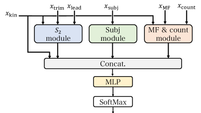
Figure 2: A schematic diagram of our AM combining $x_{\mathrm{kin}}$ (Section 2.2), $x_{S_{2}}=x_{\mathrm{trim}},x_{\mathrm{lead}}$ (Section 2.3), $x_{\mathrm{count}}$ and $x_{\mathrm{MF}}$ (Section 2.4), and $x_{\mathrm{subj}}$ (Section 2.5) for the inference.

In the following subsections, we describe each of the HLFs and their analysis modules. Figure 2 shows a schematic diagram of the AM combining the HLFs motivated from the following.

• (Section 2.2) jet kinematics, $x_{\mathrm{kin}}$.

• (Section 2.3) IRC-safe energy correlations, $x_{S_{2}}=\{x_{\mathrm{trim}},x_{\mathrm{lead}}\}$ Lim:2018toa ; Chakraborty:2019imr ; Chakraborty:2020yfc .

• (Section 2.4) jet color charge: $p_{T}$-scale conditioned jet constituent multiplicity distribution $x_{\mathrm{count}}$ and its generalization $x_{\mathrm{MF}}$ Chakraborty:2020yfc ; Lim:2020igi .

• (Section 2.5) subjet momenta $x_{\mathrm{subj}}$ and its constituent multiplicity for its color charge $x_{\mathrm{subj}}^{ex}$.

The $p_{T}$-conditioned constituent multiplicities $x_{\mathrm{count}}$ and the last subjet analysis module are the main new features of this paper. In Section 3, we will show that the jet classifier built from AM performs nearly equal to ParT. Namely, the selected HLFs are sufficient for describing the top jet classifier based on ParT. This setup further allows us to determine which features are more relevant in the classification by comparing tagging performance when some HLFs are dropped.

2.2 Global Features: Basic Jet Kinematics

We first select the global features $x_{\mathrm{kin}}$ mainly to provide characteristic angular scales of jets, which are given by the ratio of jet mass $m$ and transverse momentum $p_{T}$ to all the analysis modules. In particular, we use the kinematical variables of the whole jet $\mathrm{\mathbf{J}}$ and the trimmed jet $\mathrm{\mathbf{J}}_{\mathrm{trim}}$to capture the angular scale of top quark decay. We additionally provide the variables of the leading $p_{T}$ subjet $\mathrm{\mathbf{J}}_{\mathrm{lead}}$ to implicitly capture the W-boson decay scale. The resulting global features consist of the following inputs:

$$x_{\mathrm{kin}}=(p_{T,\mathrm{\mathbf{J}}},m_{\mathrm{\mathbf{J}}},p_{T,\mathrm{\mathbf{J}}_{\mathrm{trim}}},m_{\mathrm{\mathbf{J}}_{\mathrm{trim}}},p_{T,\mathrm{\mathbf{J}}_{\mathrm{lead}}},m_{\mathrm{\mathbf{J}}_{\mathrm{lead}}}).$$ (3)

2.3 IRC-Safe Energy Correlators: Relation Network and Two-Point Energy Correlation Spectrum

The topological features and color charge characteristics are often captured by IRC safe energy correlators Tkachov:1995kk , for example, $N$-subjettiness Thaler:2010tr and jet width/girth Gallicchio:2011xq . To build an analysis module covering the topological and color charge features described by the energy correlators, we use a relation network (RN) with IRC safety constraint Lim:2018toa .

The vanilla RN DBLP:journals/corr/RaposoSBPLB17 ; NIPS2017_7082 is a fully connected graph neural network that only uses edge features between vertices. Since perturbative phenomena in jets, such as particle decays and parton showers, are often described by two-body kinematics, an RN is a good choice for the first feature extraction. The RN consists of two networks: $\Phi_{E}$ for modeling derived edge features between two vertices and $\Phi_{G}$ for mapping accumulated edge features to the global output feature. The network output is then written as follows:

$$\Phi^{G}\left[\sum_{i\in a,j\in b}\Phi^{E}(v_{i},v_{j})\right],$$ (4)

where $v_{i}$ and $v_{j}$ are the vertex features, and the sum runs over all the vertices representing jet constituents in sets $a$ and $b$.

With IRC safety and additional translation and rotation invariances on the $(\eta,\phi)$ plane, the summand must be a two-point energy correlator with angular weighting function $W(R)$ that solely depends on the relative distance between two constituents $R_{ij}=\sqrt{(\eta_{i}-\eta_{j})^{2}+(\phi_{i}-\phi_{j})^{2}}$, i.e.,

$$\sum_{i\in a,j\in b}\Phi^{E}(v_{i},v_{j})=\sum_{i\in a,j\in b}p_{T,i}p_{T,j}W(R_{ij}).$$ (5)

This RN can be significantly simplified by introducing an IRC safe two-point correlation spectrum Lim:2020igi ; Chakraborty:2020yfc ; Lim:2018toa ; Chakraborty:2019imr ,

$$S_{2,ab}(R)=\sum_{i\in a,j\in b}p_{T,i}p_{T,j}\delta(R-R_{ij}).$$ (6)

The term $S_{2,ab}(R)\,dR$ can be interpreted as a $p_{T,i}p_{T,j}$ weighted histogram of the angular distance of jet constituent pairs. The double summations in edge feature accumulation are then simplified to a single integral,

$$\sum_{i\in a,j\in b}\Phi^{E}(v_{i},v_{j})=\int dR\;S_{2,ab}(R)W(R).$$ (7)

Note that this expression covers two-point energy flow polynomials $\mathrm{EFP}^{n}_{2}$ Komiske:2017aww ; Komiske:2018cqr when the angular weighting function $W(R)$ is a polynomial. We evaluate the integral with a simple rectangle rule with finite bin size $\Delta R=0.1$; the integral turns into a linear combination of binned two-point energy correlation spectrum $S_{2,ab}(R;\Delta R)=\int_{R}^{R+\Delta R}dR\,S_{2,ab}(R)$. The linear combination coefficients can then be absorbed into the weight matrix of the first linear layer in $\Phi_{G}$. The RN simplifies an MLP by taking $S_{2,ab}(R;\Delta R)$’s as inputs.

We again employ the trimmed jet $\mathrm{\mathbf{J}}_{\mathrm{trim}}$ and leading $p_{T}$ subjet $\mathrm{\mathbf{J}}_{\mathrm{lead}}$ for the constituent subsets to explicitly capture correlations in hard vs. soft radiations and the leading jet vs. others, respectively. In the $\mathrm{\mathbf{J}}_{\mathrm{trim}}$ analysis module, we use $a,b\in\{\mathrm{\mathbf{J}}_{\mathrm{trim}},\mathrm{\mathbf{J}}_{\mathrm{trim}}^{c}=\mathrm{\mathbf{J}}-\mathrm{\mathbf{J}}_{\mathrm{trim}}\}$ and denote the set of binned $S_{2,ab}$’s as $x_{\mathrm{trim}}$. Similarly in the $\mathrm{\mathbf{J}}_{\mathrm{lead}}$ analysis module, we use $a,b\in\{\mathrm{\mathbf{J}}_{\mathrm{lead}},\mathrm{\mathbf{J}}^{c}_{\mathrm{lead}}=\mathrm{\mathbf{J}}-\mathrm{\mathbf{J}}_{\mathrm{lead}}\}$ and refer the set of binned $S_{2,ab}$’s as $x_{\mathrm{lead}}$. It is noteworthy that the complementary sets $\mathrm{\mathbf{J}}_{\mathrm{trim}}^{c}$ and $\mathrm{\mathbf{J}}^{c}_{\mathrm{lead}}$ are formally IRC safe, and they provide a different perspective on the distribution of soft particles. We represent the output of the two analysis modules as $z_{\mathrm{trim}}$ and $z_{\mathrm{lead}}$,

$$z_{\mathrm{trim}} = \Phi^{\mathrm{trim}}(x_{\mathrm{trim}},x_{\mathrm{kin}}),$$ (8)

$$z_{\mathrm{lead}} = \Phi^{\mathrm{lead}}(x_{\mathrm{lead}},x_{\mathrm{kin}}).$$ (9)

The RNs $\Phi^{\mathrm{trim}}$ and $\Phi^{\mathrm{lead}}$ are modeled using MLPs with two hidden layers. The schematic structure of the networks is illustrated in Figure 3.

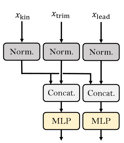
(a)

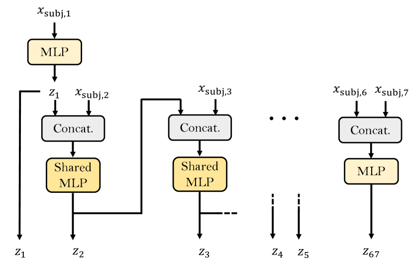
(b)

Figure 3: (a) A schematic diagram of relation network. (b) A schematic diagram of recurrent neural network analyzing subjet constituent multiplicities and subjet kinematics.

2.4 Constituent Multiplicity Distributions and Mathematical Morphology

To fully capture the color-related characteristics of jets, the IRC-safe shape variables alone are not enough; we also need IRC-unsafe variables. For instance, counting variables play a crucial role in the quark vs. gluon jet classification problem, where the distinguishing feature is the color charge of originating parton: color triplet or octet PhysRevD.44.2025 ; Gallicchio:2011xq ; Frye:2017yrw . Such counting variables are also essential in top jet tagging, as quark vs. gluon jet classification is needed at the subjet level. Note that the kinematics of subjets are different in top jets and QCD jets; the quark subjets of top jets tend to have similar starting $p_{T}$ scale, whereas those of QCD jets do not, due to the kinematics of parton shower. This kinematic difference in subjets suggests that conditional distributions of the counting variable given jet constituent $p_{T}$ can be an informative variable for capturing those color substructures of subjets.

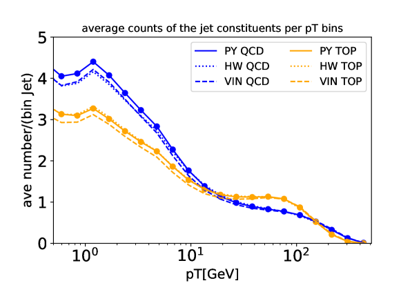
Figure 4: Average counts of the jet constituents per $p_{T}$ bins for top and QCD jet samples. The jet constituents are Delphes Eflow objects of QCD or top jets pixellated with the size $\Delta=0.1\times 0.1$. The bin boundaries are at $p_{T}=[0.1$, $0.5\times(\sqrt{2})^{k}$ ($k=0$,..), $512$] GeV. See Section 3.1 for our event sample and pre-processing details.

Figure 4 shows the expected count histogram of jet constituent $p_{T}$, averaged over our training samples. (See Section 3.1 for the detailed information on our datasets.) Results from three event generators – Pythia (PY), Herwig (HW), and Vincia (VIN) – are represented by solid, dotted, and dashed lines, respectively.

In the figure, QCD jet distributions are shown in blue lines. The HW and VIN expectations have similar trends, while PY produces slightly more constituents overall. The cases of top jets are shown in yellow lines; the PY and HW expectations are similar, while the VIN curve is slightly lower than the others. Note that the difference between event generators is more prominent in the soft region as this region is more sensitive to the parton shower, hadronization modeling, and their simulation tuning.

The differences in expectations between the QCD and top jets are more significant than the above systematic uncertainties between the simulations. In the low $p_{T}$ region, QCD jets typically have more constituents than top jets due to gluon (sub)jets and the high mass selection. On the other hand, the high $p_{T}$ region captures features of the hard process. The top jet histogram notably shows a prominent bump at $\sim 50$ GeV. This bump is mostly due to the subjets originating from the $W$ boson and the hadronization of the corresponding boosted $q\bar{q}$ system. This multiplicity distribution conditioned on $p_{T}$ captures the differences between top and QCD jets and the systematic differences between simulations. Including this histogram and its generalization for the AM will significantly enhance the information encoding performance.

One can further extend the analysis of counting information by using Minkowski Functionals (MFs) in mathematical morphology. MFs are complete linear basis functions of geometric measures with a notion of size, including the constituent multiplicity. If we use the MFs as inputs to an MLP, the resulting network effectively becomes a module analyzing geometric measures. The first linear layer models geometric measures, and the subsequent layers take care of its non-linear transformation. This method of constructing an analysis module is similar to the previously discussed simplification of RN with IRC safety constant. For analyzing jet constituent distributions on the two-dimensional $(\eta,\phi)$ plane, we need to consider the three MFs: area $A$, perimeter length $L$, and Euler characteristic $\chi$.

These MFs are used with dilation operation to encode non-trivial changes in the topology and geometry appearing at various scales, similar to persistence homology in topological data analysis 10.3389/frai.2021.667963 . Let us define a dilated image $\mathcal{I}(R)$ as a Minkowski sum of the set of constituents $\mathcal{C}$ and a disk $B(R)$ with radius $R$, i.e.,

$$\mathcal{I}(R)=\mathcal{C}+B(R)=\{a+b\,|\,a\in\mathcal{C},b\in B(R)\}.$$ (10)

We illustrate this dilation operation in Figure 5. The corresponding MFs of $\mathcal{I}(R)$ are denoted as $A(R)$, $L(R)$, and $\chi(R)$. By construction, these MFs are translation and rotation invariant.

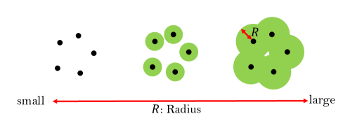
Figure 5: An illustration of the dilation of point clouds by disks. This dilation is used before evaluating the Minkowski Functionals.

The persistence analysis on MFs under the dilation captures changes in topology and geometry. When the dilation is sufficiently small, the MFs of the dilated image are described by Steiner’s formula, i.e., the dilated MFs are linear combinations of MFs without dilation, i.e., dots. For example, consider the dilation from left to middle of Figure 5 just before the disks touch each other. The MFs, in this case, can be expressed as follows.

$$A(R)=\pi R^{2}\cdot\chi(0),\quad L(R)=2\pi R\cdot\chi(0),\quad\mathrm{and}\;\chi(R)=\chi(0).$$ (11)

However, as soon as the disks come in contact, this relationship no longer holds, indicating that a non-trivial topological change occurred at the dilation scale. The MFs after the dilations are computed using shapely package Gillies_Shapely_2023 based on GEOS library libgeos . For the numerical evaluations, the disks are approximated by regular 64-sided polygons.

To make this persistence analysis conditioned on constituent $p_{T}$, we examine the MFs of jet constituents exceeding certain $p_{T}$ thresholds $p_{T}^{\mathrm{th}}$. This setup yields MFs – $A(R;p_{T}^{\mathrm{th}})$, $L(R;p_{T}^{\mathrm{th}})$, and $\chi(R;p_{T}^{\mathrm{th}})$ – as functions of disk radius $R$ and the threshold $p_{T}^{\mathrm{th}}$. These functions can simultaneously capture the morphology of soft constituents and hard substructures within the jet. The MFs are sampled at the following values of $R$ and $p_{T}^{\mathrm{th}}$ to create a discrete set of network inputs.

$$R \in \left.\begin{cases}0.025k+\epsilon&k=1,\cdots,8\\ 0.2+0.05(k-8)+\epsilon&k=9,\;10\end{cases}\right\}$$

$$p^{\mathrm{th}}_{T} \in \left\{0,1,2,4,8\right\}\;\mathrm{GeV}.$$ (12)

Here, $\epsilon$ is a small positive number to avoid the numerical instability appearing when two disks overlap only at the boundary.

Note that the diameter $2R$ is the parameter describing the correlation scale in this persistence analysis. The first MFs with $R=0.025$ are simply the constituent multiplicities since we are using angular resolution $0.1$ and no disks are overlapping each other; the MFs will be simply given as Eq. 11. For $k>1$, some disks may overlap, and MFs can capture non-trivial topological changes during the dilation. For $R>0.2$, we switch to a coarser grid. Most small-scale effects are smeared out at this scale, leaving only large-scale information less sensitive to the $R$ choice, such as hard substructure and large-angle radiations. We limit the angular scale up to $R=0.3$ in this paper.

In summary, this jet morphology analysis module covering IRC-unsafe counting observables considers the following inputs:

• $x_{\mathrm{count}}$: the values of jet constituent histogram bins over constituent $p_{T}$ within 0.1 GeV to 50 GeV. We use the following bin edges scaling exponentially:

  $$\left[0.1,\;a_{1},\;\cdots,\;a_{n_{\mathrm{bins}}-1},\;a_{n_{\mathrm{bins}}}=50\right]\;\mathrm{GeV},\quad a_{k}=0.5\cdot 10^{2(k-1)/(n_{\mathrm{bins}}-1)}\;$$ (13)

  We use $n_{\mathrm{bins}}=20$ bins for this analysis module.

• $x_{\mathrm{MF}}$: $A(R;p_{T}^{\mathrm{th}})$, $L(R;p_{T}^{\mathrm{th}})$, and $\chi(R;p_{T}^{\mathrm{th}})$ evaluated at points described in Eq. 12 with $R\leq 0.3$.

We simply use an MLP $\Phi^{\mathrm{MF}}$ to analyze these inputs. The outputs $z_{\mathrm{MF}}$ are given as follows.

$$z_{\mathrm{MF}}=\Phi^{\mathrm{MF}}(x_{\mathrm{count}},x_{\mathrm{MF}},x_{\mathrm{kin}}).$$ (14)

2.5 Recursive Neural Network for Subjet Constituent Multiplicities and Kinematics

The analysis of constituent multiplicity and Minkowkski functional conditioned on $p_{T}$ provides information regarding the color charge of jets and its morphological behavior at each $p_{T}$ scale. This approach implicitly captures the information about subjet color charges. However, a few ambiguous cases exist, especially when two subjets have a similar $p_{T}$ scale. To address this ambiguity, we introduce an analysis module for dealing with subjet constituent multiplicity explicitly.

In our subjet analysis module, we focus on seven leading $p_{T}$ Cambridge-Aachen subjets Dokshitzer:1997in ; Wobisch:1998wt with radii of 0.1, 0.2, and 0.3. This is because the angular resolution of inputs is 0.1, and other modules handle larger angular scales. The choice of seven subjets is motivated by the results of $n$-subjettiness based taggers Datta:2017rhs . As the subjettiness analysis for top jet tagging saturates at 5-body analysis Moore:2018lsr , considering seven subjets allows us to account for a few additional soft radiations.

We consider the following sets of features for each $k$-th subjet with radius $R$.

$$x^{\mathrm{(ex)}}_{\mathrm{subj},k,R} = \{p_{k},N_{c,k}\}$$ (15)

$$x_{\mathrm{subj},k,R} = \{p_{k}\}$$ (16)

Here, $p_{k}$ is the subjet 4-momentum, and $N_{c,k}$ denotes the number of constituents in the subjet. For simplicity, we do not use the full Minkowski functionals; the $N_{c,k}$ alone provides sufficient information when this module operates together with the others.

We will analyze the above subjet features $x^{\mathrm{(ex)}}_{\mathrm{subj},k,R}$ in a sequential setup to emphasize the subjet ordering, particularly because the first three subjets in top jets are likely to be quark jets. For this purpose, we stack the features of $k$-th subjets with different radii as follows,

$$x^{\mathrm{(ex)}}_{\mathrm{subj},k}=\begin{cases}\{x^{\mathrm{(ex)}}_{\mathrm{subj},k,R}\;|\;{R=0.1,0.2,0.3}\}&\textrm{for}\;k\leq 5\\ \{x_{\mathrm{subj},k,R}\;|\;{R=0.1,0.2}\}&\textrm{for}\;k=6,7.\end{cases}$$ (17)

For the 6th and 7th subjets, we omit $R=0.3$ since the preceding subjets sufficiently cover most of the jets constituents, and the remaining are again minor clusters. We also consider $N_{c,k}$ only in the first five subjets as subsequent subjets are soft subjets, and their color charge is less relevant. A simpler input set $x_{\mathrm{subj},k}$ without constituent multiplicities is also introduced for comparison,

$$x_{\mathrm{subj},k}=\{x_{\mathrm{subj},k,R}\;|\;{R=0.1,0.2}\}\ \textrm{for}\;k\leq 7.$$ (18)

To effectively accommodate the subjet features into our AM, we use a recursive neural network for the first five subjets, structured as follows:

$$z_{1} = \Phi^{\mathrm{1}}(x^{\mathrm{(ex)}}_{\mathrm{subj},1},x_{\mathrm{kin}})$$ (19)

$$z_{k} = \Phi^{\mathrm{C}}(z_{\mathrm{k}-1},x^{\mathrm{(ex)}}_{\mathrm{subj},k},x_{\mathrm{kin}})\quad\mathrm{for}\;k=2,\cdots,5.$$ (20)

Here, each $\Phi^{\mathrm{C}}$ represents a shared MLP with two hidden layers common for $k=2,\cdots,5$. The 6th and 7th subjets contain less hierarchically important information; we use a separate MLP $\Phi^{\mathrm{67}}$ with two hidden layers to process the information.

$$z_{67}=\Phi^{\mathrm{67}}(x_{\mathrm{subj},6},x_{\mathrm{subj},7},x_{\mathrm{kin}}).$$ (21)

The final output sequence of this subjet analysis module, $z_{\mathrm{subj}}$, is defined as follows.

$$z^{\mathrm{(ex)}}_{\mathrm{subj}}=(z_{1},\cdots,z_{5},z_{67}),$$ (22)

where $z^{\mathrm{(ex)}}_{\mathrm{subj}}$ corresponds to $x^{\mathrm{(ex)}}_{\mathrm{subj},k}$ inputs respectively. Figure 3 illustrates the schematic diagram of this network configuration. Note that if we use a deep set architecture NIPS2017_f22e4747 to introduce permutation symmetry for this analyzing module, the resulting network is a variant of the jet flow network Athanasakos:2023fhq with additional subjet constituent multiplicity information.

3 Comparing Classification Performances of Analysis Model and Particle Transformer

3.1 Datasets

In this section, we explain top jet and QCD jet datasets used for training jet classifiers. Top jets are sampled from the hard process $pp\rightarrow t\bar{t}$, and QCD jets are from $pp\rightarrow jj$. Both processes are simulated at a center-of-mass energy $\sqrt{s}=13$ TeV using MadGraph5 3.4.2 Alwall:2014hca . The simulated top quarks are decayed hadronically using madspin Artoisenet:2012st . To focus on generating samples for boosted top jet classification, we exclusively generate events where the transverse momentum of top quarks in $t\bar{t}$ events and leading $p_{T}$ quark/gluon in dijet events is greater than 450 GeV.

For the parton shower and hadronization simulations, we use Pythia 8.308 Bierlich:2022pfr and Herwig 7.2 Bellm:2019zci , considering the following parton shower models,

• Pythia, simple shower, (denoted as PY)

• Pythia, Vincia shower, (denoted as VIN)

• Herwig, default shower, (denoted as HW)

Vincia shower Ritzmann:2012ca ; Fischer:2016vfv is a $p_{T}$-ordered parton shower model for QCD + QED/EW showers based on the antenna formalism. This model exhibits improved color-coherence effects relative to the default simple shower model of Pythia. We additionally include Vincia to assess whether our AM has enough sensitivity to distinguish different Monte Carlo simulations, particularly in PY vs. VIN comparisons. Detailed results are presented in Appendix A. Regarding the simulation tune settings, the Monash tune Skands:2014pea is used for Pythia, and the default tune is used for Herwig. Furthermore, we simulate neutral pion decay to ensure accurate modeling of particle distribution at angular scales near 0.1.

The generated particle-level events are processed using the Delphes detector simulation deFavereau:2013fsa using the default ATLAS detector card with a modification: jets are reconstructed from EFlow objects deFavereau:2013fsa ; DeRoeck:2005sqi . The jets are reconstructed by the anti-kt algorithm Cacciari:2008gp with radius parameter $R=1$, which is implemented in fastjet Cacciari:2011ma ; Cacciari:2005hq . Note that the EFlow objects include information from tracks and electromagnetic calorimeters, offering a better angular resolution than hadronic calorimeter towers. However, to compare network architectures at the same lower angular scale threshold, we will later mask out the shorter-scale information during the construction of HLFs for AM and LLFs for ParT.

We select the leading $p_{T}$ jets with transverse momentum $p_{T,J}\in[500,600]$ GeV, jet mass $m_{J}\in[150,200]$ GeV, and pseudorapidity $|\eta|\leq 2$ as our top jet and QCD jet samples. For top jets, we further require that all quarks originating from the top and W boson decay are located within a distance $R=1$ from the jet axis on the $(\eta,\phi)$-plane. We denote the PY, VIN, and HW simulated QCD jet datasets as $\mathrm{P_{Q}}$, $\mathrm{V_{Q}}$, and $\mathrm{H_{Q}}$, respectively. Similarly, we use $\mathrm{P_{T}}$, $\mathrm{V_{T}}$, and $\mathrm{H_{T}}$ to represent PY, VIN, and HW $t\bar{t}$ datasets, respectively. The training and test dataset sizes are listed in Table 1. While the dataset sizes are not uniform, we ensure the class balance by downsampling the larger dataset so that both classes have the same number of samples during the training. However, during testing, we use the entire dataset without downsampling.

Note that the dataset sizes are bigger than the public top tagging challenge dataset Kasieczka:2019dbj ; kasieczka_2019_2603256 in a similar kinematic range. The community challenge dataset, covering a slightly different $p_{T,J}$ range of $[550,650]$ GeV, does not include preselection based on jet mass. The number of top (QCD) training dataset in the jet mass $\in[150,200]$ GeV is 476K (59K), while our QCD training datasets have about 400K samples. Our dataset has more QCD jets in this mass range, which helps to mitigate the class imbalance during the training.

	$\mathrm{P_{T}}$	$\mathrm{P_{Q}}$	$\mathrm{H_{T}}$	$\mathrm{H_{Q}}$	$\mathrm{V_{T}}$	$\mathrm{V_{Q}}$
Number of training data	524K	384K	395K	418K	403K	329K
Number of testing data	527K	388K	393K	417K	403K	328K

Table 1: The number of training and testing samples generated by Pythia (P), Herwig (H), and Vincia (V). The subscripts T and Q denote top jet and QCD jet samples, respectively. During the training of a binary classifier, we ensure the use of an equal number of samples for both classes by downsampling the larger dataset. Still, all available samples are used for testing.

3.2 Particle Transformer

We will mainly compare our AM results with the Particle Transformer (ParT) Qu:2022mxj . ParT is a transformer-based neural network NIPS2017_3f5ee243 that directly analyzes low-level features (LLFs) of jet constituents. The ParT architecture consists of three main modules:

• Particle attention blocks Qu:2022mxj , which analyze LLFs. This module is based on NormFormer architecture shleifer2021normformer with augmented multi-head attention layers. The query-key inner product in the attention layers is augmented by pairwise features inspired by LundNet Dreyer:2020brq .

• Class attention blocks Touvron_2021_ICCV that transform a trainable class token dosovitskiy2021an ; devlin2018bert into an output, utilizing the final output of the particle attention blocks.

• An MLP that converts the transformed class token into classifier outputs.

The final output of ParT is then trained by minimizing the binary cross-entropy loss function.

Since our aim is to compare classifier performance with inputs having a finite angular resolution $0.1$, we will mask out small-scale information by utilizing jet images Cogan:2014oua ; Almeida:2015jua ; deOliveira:2015xxd . The jet constituents are first preprocessed as described in Lim:2020igi . This preprocessing involves shifting, rotating, and flipping on the $(\eta,\phi)$ coordinate to ensure that the leading subjet is at the origin, the second subjet lies on the positive $\phi$-axis ($\eta=0$ and $\phi>0$), and the third subjet is on the right side of the plane ($\eta>0$). After the preprocessing, the jet constituents are pixelated into bins of size $\Delta\eta=\Delta\phi=0.1$. Pixels with non-zero energy deposits are converted into massless 4-momenta using their $(\eta,\phi)$ coordinates and energy deposits. This set of 4-momenta is used as ParT inputs.

As a result of the pixelation process, the inputs become relatively simpler than the original 4-momenta; therefore, we use a smaller version of ParT compared to the one presented in the original paper Qu:2022mxj . Given that our sample size is about 380k per class, we target a similar number of network parameters in order to maintain a positive degree of freedom. Specifically, we halve the number of attention blocks and the width of each neural network from the default setting. In this configuration, ParT has 340k parameters.

3.3 Comparing Analysis Model and Particle Transformer

3.3.1 Comparing Classification Performance

In this subsection, we compare the classification performance between AM and ParT, specifically using samples generated by PY and HW. The results involving samples generated by VIN are presented in Appendix A.

We particularly focus on the following four classification problems: ($\mathrm{P_{T}}$ vs. $\mathrm{P_{Q}}$), ($\mathrm{H_{T}}$ vs. $\mathrm{H_{Q}}$), ($\mathrm{P_{Q}}$ vs. $\mathrm{H_{Q}}$), and ($\mathrm{P_{T}}$ vs. $\mathrm{H_{T}}$). The first two, ($\mathrm{P_{T}}$ vs. $\mathrm{P_{Q}}$) and ($\mathrm{H_{T}}$ vs. $\mathrm{H_{Q}}$), are the top jet tagging problems using samples generated by PY and HW, respectively. Comparing these two will provide insight into the generator-dependency of taggers. The latter two, ($\mathrm{P_{Q}}$ vs. $\mathrm{H_{Q}}$) and ($\mathrm{P_{T}}$ vs. $\mathrm{H_{T}}$), focus on detecting differences between jets generated by PY and HW. These classifiers are trained to learn the likelihood ratio between two distinct Monte-Carlo simulations, which is crucial in quantifying differences between simulations. In this paper, our initial focus is on evaluating whether the HLFs used in AM are sufficient for effectively paralleling ParT analyzing LLFs. In-depth analyses of systematic differences using HLFs will be future works.

Model	$\mathrm{P_{T}}$ vs. $\mathrm{P_{Q}}$	$\mathrm{H_{T}}$ vs. $\mathrm{H_{Q}}$	$\mathrm{P_{Q}}$ vs. $\mathrm{H_{Q}}$	$\mathrm{P_{T}}$ vs. $\mathrm{H_{T}}$
	AUC	AUC	AUC	AUC
CNN Chakraborty:2020yfc	0.940	0.924	0.577	0.5480
IRC-safe AM-PIPs
A) $x_{\rm kin}$, $x_{S_{2}}$	0.936	0.919	0.571	0.5690
B) $x_{\rm kin}$, $x_{\mathrm{subj}}$	0.938	0.922	0.575	0.5780
C) $x_{\rm kin}$, $x_{S_{2}}$, $x_{\mathrm{subj}}$	0.941	0.925	0.579	0.5850
IRC-unsafe AM-PIPs
D) $x_{\rm kin}$, $x_{\rm MF}$, $x_{\rm count}$	0.930	0.912	0.583	0.5870
E) D) + $x_{S_{2}}$	0.941	0.925	0.595	0.5986
F) D) + $x_{S_{2}}$, $x_{\mathrm{subj}}$	0.942	0.926	0.597	0.5995
Full AM	0.943	0.928	0.600	0.6050
ParT Qu:2022mxj	0.944	0.929	0.599	0.6270

Table 2: AUC for CNN, ParT, AM, and various configurations of AM-PIPs. The specific inputs activated in each AM-PIP are listed in the left column. The AUC of AM is closest to ParT in all classifications, except for $\mathrm{P_{T}}$ vs. $\mathrm{H_{T}}$. Note that $x_{\mathrm{subj}}$ does not include subjet constituent multiplicities, while the full AM uses $x^{\mathrm{ex}}_{\mathrm{subj}}$ that includes the multiplicities.

Model	$\mathrm{P_{T}}$ vs. $\mathrm{P_{Q}}$		$\mathrm{H_{T}}$ vs. $\mathrm{H_{Q}}$		$\mathrm{P_{Q}}$ vs. $\mathrm{H_{Q}}$		$\mathrm{P_{T}}$ vs. $\mathrm{H_{T}}$
	$R_{50\%}$	$R_{30\%}$	$R_{50\%}$	$R_{30\%}$	$R_{50\%}$	$R_{30\%}$	$R_{50\%}$	$R_{30\%}$
CNN Chakraborty:2020yfc	79.0	318	55.9	219	2.33	4.16	2.57	4.83
IRC-safe AM-PIPs
A) $x_{\rm kin}$, $x_{S_{2}}$	71.1	276	49.1	186	2.51	4.63	2.48	4.49
B) $x_{\rm kin}$, $x_{\mathrm{subj}}$	75.3	290	52.4	203	2.53	4.75	2.58	4.74
C) $x_{\rm kin}$, $x_{S_{2}}$, $x_{\mathrm{subj}}$	80.7	316	56.0	217	2.59	4.87	2.64	4.85
IRC-unsafe AM-PIPs
D) $x_{\rm kin}$, $x_{\rm MF}$, $x_{\rm count}$	57.8	215	40.8	152	2.61	4.96	2.65	4.96
E) D) + $x_{S_{2}}$	81.2	321	56.5	223	2.74	5.31	2.76	5.19
F) D) + $x_{S_{2}}$, $x_{\mathrm{subj}}$	84.8	341	58.9	234	2.76	5.36	2.78	5.21
Full AM	85.7	343	61.3	244	2.78	5.43	2.82	5.36
ParT Qu:2022mxj	90.5	372	62.6	242	2.77	5.38	3.07	5.94

Table 3: Rejection rates $R_{X\%}$ for CNN, ParT, AM, and various configurations of AM-PIPs. The specific inputs activated in each AM-PIP are listed in the left column. Note that $x_{\mathrm{subj}}$ does not include subjet constituent multiplicities, while the full AM uses $x^{\mathrm{ex}}_{\mathrm{subj}}$ that includes the multiplicities.

We present the classification performances of AMs and ParT in terms of AUC in Table 2, and two rejection rates $R_{50\%}$ and $R_{30\%}$ in Table 3. The rejection rate $R_{X\%}$ defined as follows:

$$R_{X\%}=1/\mathrm{FPR}\ \mathrm{at\ TPR}=X\%,$$ (23)

where TPR is the true positive rate, and FPR is the false positive rate. In this comparison, the first class is assumed to be the positive class, and the second class is considered the negative class. We report the performance metrics of AM and ParT that achieved the best AUC, selected from six AM and ten ParT trainings, each of them trained with different random seeds, respectively.

In Table 2, we see that AM performs almost as well as ParT in our classification tasks, except for the ($\mathrm{P_{T}}$ vs. $\mathrm{H_{T}}$) classification. We will discuss the significance of the differences in ($\mathrm{P_{T}}$ vs. $\mathrm{H_{T}}$) later. The AUCs for top jet tagging are similar, and AM’s AUC is even a bit higher in ($\mathrm{P_{Q}}$ vs. $\mathrm{H_{Q}}$), even though it only uses a few HLFs. However, when AUCs are close, the corresponding ROC curves may intersect at some point. AUC alone may not clearly determine the performance hierarchy in these cases.

The rejection rates in Table 3 are more precise measures for the performance comparison. The rejection rates of ($\mathrm{P_{T}}$ vs. $\mathrm{P_{Q}}$), ($\mathrm{P_{Q}}$ vs. $\mathrm{H_{Q}}$), and ($\mathrm{P_{T}}$ vs. $\mathrm{H_{T}}$) show the same trends seen in the AUCs. But the HW top tagging problem ($\mathrm{H_{T}}$ vs. $\mathrm{H_{Q}}$), whose AUC was higher for ParT, now shows a mixed behavior: $R_{50\%}$ is better for ParT, $R_{30\%}$ is better for AM. In summary, AM and ParT show similar performances in ($\mathrm{H_{T}}$ vs. $\mathrm{H_{Q}}$), ParT slightly outperforms AM in ($\mathrm{P_{T}}$ vs. $\mathrm{H_{T}}$) and ($\mathrm{P_{T}}$ vs. $\mathrm{P_{Q}}$), but AM does slightly better in ($\mathrm{P_{Q}}$ vs. $\mathrm{H_{Q}}$). These experiments indicate that while AM and ParT are comparable in performance, their exact hierarchy is unclear. In Section 4, we will discuss the significance of the differences using bootstrap methods, but the statistical significance after counting statistical uncertainty and training stochasticity does not exceed 3$\sigma$.

We tested several modifications of the AM, especially for closing the small gap between AM and ParT in the PY top tagging problem ($\mathrm{P_{T}}$ vs. $\mathrm{P_{Q}}$), although HW top tagging and VIN top tagging (see Appendix A) do not have such a performance gap. The modification includes various adjustments such as replacing the recursive network model for $x^{\mathrm{ex}}_{\mathrm{subj}}$ to a fully connected network, adding MFs at an energy threshold of 16 GeV, increasing the hidden layer numbers from two to three, and concatenating $x_{\mathrm{kin}}$ in each layer for more explicit jet kinematics conditioning. However, these changes were insufficient to close the AUC gap. The gap exclusive to PY suggests that introducing PY-specific HLFs appearing above the hadronic calorimeter resolution could potentially close it. However, delving into HLFs specific to a particular Monte-Carlo simulation is beyond the scope of the paper, so we do not further attempt to fill the gap within this paper.

3.3.2 Importance of each Sub-module of Analysis Model

In addition to the direct comparison between AM and ParT, we further consider AM with partial inputs (AM-PIPs) for a hierarchical comparison of the inputs. Our AM incorporates selected sets of HLFs described in Section 2. These HLFs, which include jet kinematics $x_{\mathrm{kin}}$, two-point energy correlations $x_{S_{2}}$, $p_{T}$-conditioned constituent multiplicity $x_{\mathrm{count}}$, Minkowski functionals for jet morphology $x_{\mathrm{MF}}$, subjet constituent multiplicities and kinematics $x^{\mathrm{ex}}_{\mathrm{subj}}$, are designed to capture various physics features of top jets illustrated in Figure 1. To evaluate the impact of each HLF set on the classification performance, we systematically activate or deactivate specific sets of inputs and their corresponding analysis modules. This method of toggling inputs allows us a hierarchical comparison, assessing the relative efficacy of these subsets within the complete AM framework.

Besides AMs and ParT, we consider a convolutional neural network (CNN) introduced in our previous works Chakraborty:2020yfc ; Lim:2020igi . The CNN demonstrated performance similar to that of AM-PIPs with inputs ($x_{\mathrm{kin}}$, $x_{S_{2}}$, $x_{\mathrm{MF}}$). We will use its classification performances as a baseline for the following comparisons.

Table 2 and Table 3 also shows the results of AM-PIPs. The tested input configurations are: A) ($x_{\rm kin}$, $x_{S_{2}}$), B) ($x_{\rm kin}$, $x_{\mathrm{subj}}$), C) ($x_{\rm kin}$, $x_{S_{2}},x_{\mathrm{subj}}$), and D) ($x_{\rm kin}$, $x_{\rm MF}$, $x_{\rm count}$), E) ($x_{\rm kin}$, $x_{S_{2}}$, $x_{\rm MF}$, $x_{\rm count}$), and F) ($x_{\rm kin}$, $x_{S_{2}}$, $x_{\mathrm{subj}}$, $x_{\mathrm{MF}}$, $x_{\rm count}$). These configurations allow us to assess the impact of different HLF combinations on the classification performance. Full AM outperforms all AM-PIPs, indicating that all the HLF sets contain independent information that AM can utilize effectively. Furthermore, the consistent improvement observed with the additional HLFs indicates that the statistical uncertainties are less significant in the performance comparison among AM-PIPs.

The first three AM-PIPs, configuration A), B), and C), omit the counting variables, making them less sensitive to the IRC-unsafe features. Each sub-module alone demonstrates effectiveness in the classifications, as shown in the A) and B) results. But configuration C), combining the two-point energy correlations and subjet kinematics information, performs better, and its performance marginally surpasses that of CNN. Note that CNN is essentially an extension of a local pointwise feature aggregator lin2013network , and its design does not prioritize features from a certain location during aggregation. In contrast, subjets have hierarchical structures. Explicitly providing the hierarchical subjet information allows the AM-PIP to outperform CNN since we have provided additional information.

The latter three AM-PIPs, configuration D), E), and F), discuss IRC-unsafe features. We first observe that the performance drops significantly in the top tagging problems ($\mathrm{P_{Q}}$ vs. $\mathrm{H_{Q}}$) and ($\mathrm{P_{T}}$ vs. $\mathrm{H_{T}}$) if we restrict AM to access only to constituent multiplicities and topological and morphological features as in the configuration D). The performance is even worse than CNN. Note that MFs are geometric measures, so they are specialized in measuring sizes rather than measuring relative positions, even though scale-dependent MF analysis helps analyze the relative structures at some level. Identifying the local clusters and their relative structure is very important in top tagging, so CNN performs better than the configuration D). These observations show that IRC safe features for analyzing the structure of jets, such as $x_{S_{2}}$ and $x_{\mathrm{subj}}$, are important in top tagging problems using samples from the same generators.

But in the case of comparing simulated jets from different Monte Carlo simulations, ($\mathrm{P_{T}}$ vs. $\mathrm{P_{Q}}$) and ($\mathrm{H_{T}}$ vs. $\mathrm{H_{Q}}$), the setup D) starts to outperform the IRC-safe AM-PIPs. The difference between simulated jets is more prominent in IRC-unsafe features because they have significant simulation model dependence, so D) can distinguish jets from different simulations more clearly than the others. Considering this, orthogonal information improves the performance. The setup D) is even performing better than CNN in this case, contrary to what we observed in the top tagging problems. The overall geometry of particle distribution is more important than hard substructures for distinguishing Monte Carlo simulations. Although CNN structure can cover MFs Lim:2020igi in the large depth limit, using MFs explicitly could help gain performances compared to CNN with moderate depth.

The last comparison among E), F), full AM, and ParT justifies the importance of subjet kinematics and their color structures. The baseline of this comparison is E), which is the AM-PIP without subjet information. Including subjet kinematic information $x_{\mathrm{subj}}$ to E) slightly improves performance, as seen in F). The reason is that two-point energy correlations, counting observables, and Minkowski functionals treat all the constituents equally during the feature aggregation while subjet information is not. However, the performance of F) still does not closely match that of ParT. Further considering subjet constituent multiplicities makes F) to the full AM, whose performance is comparable to ParT as discussed in the previous sections. This shows the colors of subjets, i.e., the origin of the subjets ($q$ or $g$), plays a certain role in the classifications.

4 Statistical Significance of the Difference between Analysis Model and Particle Transformer

Model	$\mathrm{P_{T}}$ vs. $\mathrm{P_{Q}}$
	AUC	$R_{50\%}$	$R_{30\%}$
ParT-best (as I)	0.9425$\pm$0.0005	85$\pm$2($\pm 1$)	327$\pm$12($\pm 9$)
ParT-2nd (as II)	0.9420$\pm$0.0010	83$\pm$3($\pm 1$)	317$\pm$14($\pm 9$)
AM (as II)	0.9396$\pm$0.0006	77$\pm$2($\pm 1$)	296$\pm$12($\pm 8$)
Model	$\mathrm{H_{T}}$ vs. $\mathrm{H_{Q}}$
	AUC	$R_{50\%}$	$R_{30\%}$
ParT-best (as I)	0.9266$\pm$0.0009	59.0$\pm$2.0($\pm 0.7$)	222$\pm$10($\pm 5$)
ParT-2nd (as II)	0.9265$\pm$0.0008	58.0$\pm$2.0($\pm 0.7$)	225$\pm$08($\pm 5$)
AM (as II)	0.9240$\pm$0.0005	55.2$\pm$0.7($\pm 0.6$)	218$\pm$06($\pm 5$)
Model	$\mathrm{P_{Q}}$ vs. $\mathrm{H_{Q}}$
	AUC	$R_{50\%}$	$R_{30\%}$
ParT-best (as I)	0.5920$\pm$0.0040	2.700$\pm$0.040($\pm 0.006$)	5.20$\pm$0.10($\pm 0.02$)
ParT-2nd (as II)	0.5910$\pm$0.0040	2.700$\pm$0.040($\pm 0.006$)	5.14$\pm$0.08($\pm 0.02$)
AM (as II)	0.5949$\pm$0.0006	2.732$\pm$0.005($\pm 0.006$)	5.27$\pm$0.02($\pm 0.02$)
Model	$\mathrm{P_{T}}$ vs. $\mathrm{H_{T}}$
	AUC	$R_{50\%}$	$R_{30\%}$
ParT-best (as I)	0.614$\pm$0.006	2.92$\pm$0.06($\pm 0.01$)	5.60$\pm$0.10($\pm 0.02$)
ParT-2nd (as II)	0.613$\pm$0.007	2.91$\pm$0.08($\pm 0.01$)	5.60$\pm$0.20($\pm 0.02$)
AM (as II)	0.598$\pm$0.001	2.75$\pm$0.01($\pm 0.01$)	5.17$\pm$0.02($\pm 0.02$)

Table 4: AUCs and rejection rates $R_{X\%}$ of the AM and ParT, both trained on bootstrap datasets. We show the average and standard deviations of these classification performance metrics. For ParT, the classifier is trained twice; the ParT with a higher average AUC is labeled as ParT-best, and the other as ParT-2nd. The numbers in brackets represent the statistical uncertainties associated with each metric. Note that the bootstrap estimated uncertainties already include this.

In Section 3, we observed that 1) AM and ParT performance are comparable, and 2) AM-PIP improves as more inputs are included. In this section, we estimate the statistical uncertainties of the performance measures to show the significance of our conclusion.

4.1 Estimating Uncertainty of Performance Metrics by Bootstrapping

We estimate uncertainties associated with network training by using the bootstrap method. This method involves the generation of bootstrap datasets from the original dataset by sampling with replacement. In this resampling procedure, we treat the empirical distribution of the training dataset as an approximate true distribution. The bootstrap datasets effectively act as representative samples of this approximate true distribution. By training networks again on each of these datasets, this bootstrap method allows us to estimate the variance of training results. For this study, we use ten bootstrap datasets. Note that our AM is computationally cheaper than ParT, so this bootstrap analysis can be done much faster. The computational resources utilized by AM and ParT are explained in Appendix B.

In Table 4, we show the average and standard deviation of AUC, $R_{50\%}$, and $R_{30\%}$ of AMs and ParTs trained on the bootstrap dataset. Here, we use the original test datasets without bootstrapping to evaluate those performance measures. Note that the performance measures are worse than those in Table 2 and Table 3. The difference is due to the bootstrap dataset being sampled from the original dataset. The resampling does not capture all the training samples, which makes the classifiers slightly suboptimal. Nevertheless, the variance is still a consistent estimator of the uncertainty. For ParT, we further validate this method by repeating the procedure with another set of bootstrap datasets. We denote the bootstrap result with a higher average AUC as the ParT-best and the other as ParT-2nd. The ParT-best and ParT-2nd results are compatible with the uncertainties.

One notable observation is that the bootstrap-estimated uncertainties for ParT are significantly larger than those for AM. Specifically, in the HW top tagging problem, the uncertainties of ParT are twice as large as those of AM. The uncertainty difference is amplified by factor 10 in the generator classifications ($\mathrm{P_{T}}$ vs. $\mathrm{H_{T}}$) and ($\mathrm{P_{Q}}$ vs. $\mathrm{H_{Q}}$). This phenomenon is due to the bias-variance tradeoff inherent in statistical modeling. More expressive models, like ParT, can model classifiers more accurately, but at the cost of increased variance in the results. Consequently, ParT requires a larger sample size to achieve the same level of statistical precision as AM; for an analysis with a given sample size, the uncertainty of AM is always expected to be smaller than that of ParT.

This precision difference becomes more prominent if we subtract the statistical uncertainty from the bootstrap estimated uncertainty. Here, we specifically focus on rejection rates, as their statistical uncertainty can be quickly estimated using analytic formulas. A naive estimation on $1\sigma$ statistical uncertainty of the false positive rate $R_{X\%}^{-1}$ is given by the Wald interval, $\sigma_{R_{X\%}^{-1}}=\sqrt{R_{X\%}^{-1}(1-R_{X\%}^{-1})/N}$, where $N$ is the number of second class samples. The uncertainty in the rejection rate, $\sigma_{R_{X\%}}$, is then derive as $\sigma_{R_{X\%}}={\sigma_{R_{X\%}^{-1}}}/{R_{X\%}^{2}}$. The statistical uncertainty estimates for the rejection rates are listed in Table 4, denoted within brackets.

We can see that the uncertainty is dominated by the statistical uncertainty in the case of AMs, whereas for ParT, this is not the case. This additional variance observed in ParT is from randomness of training, such as network initializations and batch splitting. In the case of AM, the training procedure sufficiently suppresses this initial condition and other randomness dependence in training so that the bootstrap estimated uncertainty and statistical uncertainty are approximately the same. In contrast, ParT training is less successful in reducing this variance to levels below the statistical uncertainties, resulting in higher residual variance in the bootstrap estimated uncertainties. This stability in the training process is one significant advantage of AMs, especially when their performance is comparable to that of state-of-the-art models like ParT.

metric	$\mathrm{P_{T}}$ vs. $\mathrm{P_{Q}}$	$\mathrm{H_{T}}$ vs. $\mathrm{H_{Q}}$	$\mathrm{P_{Q}}$ vs. $\mathrm{H_{Q}}$	$\mathrm{P_{T}}$ vs. $\mathrm{H_{T}}$
AUC	2.76	2.58	0.84	2.36
$R_{50\%}$	2.19	1.56	0.79	2.29
$R_{30\%}$	1.64	0.51	1.08	2.84

Table 5: Estimated significance of the difference between classifier performance metrics between AM and ParT, based on the training uncertainties measured by the bootstrap method.

For a more quantitative comparison of the difference in performance measures between AM and ParT, we define the significance of their performance measure difference as follows:

$$\sigma_{X}=\frac{|X_{\mathrm{ParT}}-X_{\mathrm{AM}}|}{\sqrt{\sigma_{X,\mathrm{ParT}}^{2}+\sigma_{X,\mathrm{AM}}^{2}}},\quad X\in\{\mathrm{AUC},R_{50\%},R_{30\%}\}.$$ (24)

For $X_{\mathrm{ParT}}$ and $\sigma_{X,\mathrm{ParT}}$, we use the average of ParT-best and Part-2nd results. The significances $\sigma_{X}$ are shown in Table 5, all of which are less than $3\sigma$. This indicates that the moderate performance gap between AM and ParT in PY top tagging ($\mathrm{P_{T}}$ vs. $\mathrm{P_{Q}}$) and top jet simulation comparison ($\mathrm{P_{T}}$ vs. $\mathrm{H_{T}}$), shown in Table 2 and Table 3, becomes less significant after accounting both statistical uncertainty and training stochasticity.

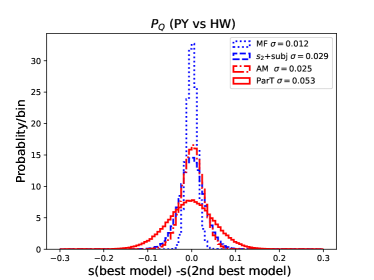
Figure 6: Distribution of the difference between the classifier outputs of the best model and the second best model for $\mathrm{P_{Q}}$ vs. $\mathrm{H_{Q}}$ classification. The red solid line is for ParT, and the red dot-dashed line is for AM. The distribution for ParT is significantly broader than that of AM. Additionally, the blue dotted line is for the AM-PIP with only the morphology analysis module active, and the blue dashed line is for the AM-PIP with relation network and subjet analysis modules active. These two blue lines are for demonstrating output variations in simpler models compared to the full AM.

Finally, to test the consistency of AM and ParT predictions under the randomness of the training, we revisit the classifiers for ($\mathrm{P_{Q}}$ vs. $\mathrm{H_{Q}}$) trained with different random seeds, as discussed in Section 3.3.1. Figure 6 illustrates the differences in classifier outputs between the networks with the best and second-best AUCs. A classifier less influenced by training randomness will yield more similar network outputs. The difference histogram will peak narrowly around zero in such a case. In this comparison, the peak for AM (red dot-dashed line) is narrower than that for ParT (red solid line), indicating more consistent predictions. Specifically, the standard deviation of the histogram is 0.03 for AM, and 0.06 for ParT. A simpler model, such as AM-PIP involving $(x_{\mathrm{kin}},x_{\mathrm{MF}},x_{\mathrm{count}})$, shows even smaller variation of 0.012, though its performance is suboptimal.

4.2 Comparing the Information Content of Classifiers using Odds Ratio

In this section, we directly compare AM and ParT using an odds ratio, which is useful in comparing the information content of two classifiers. Let $s^{\mathrm{I}}(x)$ be the classifier output for given input $x$, i.e., the posterior being a signal as modeled by classifier ${\mathrm{I}}$. The odds ratio $\hat{w}^{\mathrm{I}/\mathrm{II}}$ is defined as the ratio of odds estimated by models $\mathrm{I}$ and $\mathrm{II}$, expressed as follows:

$$\mathrm{OR}^{\mathrm{I}/\mathrm{II}}(x) = \frac{s^{\mathrm{I}}(x)}{1-s^{\mathrm{I}}(x)}\cdot\frac{1-s^{\mathrm{II}}(x)}{s^{\mathrm{II}}(x)}.$$ (25)

An odds ratio greater than 1 indicates that the classifier $\mathrm{I}$ is more confident in its signal prediction by the factor of the odds ratio than the classifier $\mathrm{II}$. If both models are identical, the odds ratio will be 1. Therefore, deviations from 1 in the odds ratio indicate differences in the predictions of the two classifiers for a given sample.

Note that when there is a clear hierarchy between two models, the odds ratio can also be interpreted as a likelihood ratio between two classes, using only the features exclusive to the more expressive model. If the classifier $\mathrm{I}$ is more expressive than $\mathrm{II}$, the prediction $s^{\mathrm{II}}(x)$ in the denominator acts as a normalizer countering information in $s^{\mathrm{I}}(x)$ covered by the model $\mathrm{II}$, similar to conditional probability. With this odds ratio interpretation, we can construct a posterior probability that works as a classifier utilizing only the features exclusive to $\mathrm{I}$:

$$s^{\mathrm{I}/\mathrm{II}}(x)=\frac{\mathrm{OR}^{\mathrm{I}/\mathrm{II}}(x)}{1+\mathrm{OR}^{\mathrm{I}/\mathrm{II}}(x)}.$$ (26)

A more detailed derivation of this interpretation is described in Appendix C.

Since the odds ratio has a classifier interpretation, we quantify the difference between AM and ParT in terms of performance metrics (AUC and rejection rates) of ROC curves using the probability $s^{\mathrm{I}/\mathrm{II}}$ (equivalently the odds ratio $\mathrm{OR}^{\mathrm{I}/\mathrm{II}}$) as a threshold variable. If two classifiers are equivalent, the AUC will be that of a random guess, 0.5, and the rejection rate $R_{X\%}$ will be $1/X\%$.

To estimate uncertainties together, we take the average prediction of the ParT-best models from the bootstrap analysis as ${s}^{\mathrm{I}}$. We then evaluate the odds ratio against AM and ParT-2nd, each trained on bootstrap datasets. Specifically, for each of the $i$-th bootstrap dataset, $s^{\mathrm{II}}$ is either the prediction of AM, $s^{\mathrm{AM}}_{i}$, or ParT-2nd, $s^{\textrm{ParT-2nd}}_{i}$. We evaluate the mean and variance of AUC and rejection rates ($R_{50\%}$ and $R_{30\%}$) across the bootstrap datasets to assess the difference between the two models.

The above uncertainty estimation procedure primarily focuses on model $\mathrm{II}$ variations and does not explicitly account for the uncertainties of model $\mathrm{I}$. To estimate the uncertainties in ParT-best, we can take ParT-2nd as $s^{\mathrm{II}}$. The uncertainties associated with ParT-2nd can be interpreted as an additional uncertainty due to the variation within ParT-best as model $\mathrm{I}$ because ParT-best and ParT-2nd are essentially the same models trained under different random states.

$\mathrm{II}$	metric	$\mathrm{P_{T}}$ vs. $\mathrm{P_{Q}}$	$\mathrm{H_{T}}$ vs. $\mathrm{H_{Q}}$	$\mathrm{P_{Q}}$ vs. $\mathrm{H_{Q}}$	$\mathrm{P_{T}}$ vs. $\mathrm{H_{T}}$
ParT-2nd	AUC	0.52$\pm$0.05	0.53$\pm$0.04	0.50$\pm$0.02	0.50$\pm$0.02
	$R_{50\%}$	2.2$\pm$0.4	2.2$\pm$0.3	2.03$\pm$0.10	2.0$\pm$0.1
	$R_{30\%}$	4.2$\pm$0.9	4.3$\pm$0.9	3.4$\pm$0.2	3.3$\pm$0.3
AM	AUC	0.48$\pm$0.02	0.47$\pm$0.01	0.507$\pm$0.003	0.546$\pm$0.003
	$R_{50\%}$	1.87$\pm$0.09	1.83$\pm$0.05	2.04$\pm$0.02	2.29$\pm$0.02
	$R_{30\%}$	3.2$\pm$0.2	3.2$\pm$0.2	3.41$\pm$0.04	3.91$\pm$0.05

Table 6: Classification performance metrics for the odds ratio $\mathrm{OR}^{\mathrm{I}/\mathrm{II}}$, where $\mathrm{I}$ is ParT-best and $\mathrm{II}$ is AM and ParT-2nd. This table uses the results from bootstrap analysis, and we show the training uncertainties together. An AUC value closer to 0.5 and rejection rates $R_{X\%}$ closer to $1/X\%$ indicates that the two classifiers have similar information contents.

In Table 6, we show the odds ratio analysis results. Ideally, the results of ParT-2nd should be those of random guess results ($\mathrm{AUC}=0.5$, $R_{50\%}=2$, and $R_{30\%}=3.33$). The rejection rates $R_{30\%}$ for the top tagging problems ($\mathrm{P_{T}}$ vs. $\mathrm{P_{Q}}$) and ($\mathrm{H_{T}}$ vs. $\mathrm{H_{Q}}$) are slightly deviate from 3.33. However, the uncertainty is also sufficiently large, so the results are consistent with the expectation. Overall, all the performance metrics are compatible with those of a random guess, and the expectation holds for all the classification tasks.

The results of AM apparently deviated from those of a random guess, especially in ($\mathrm{P_{T}}$ vs. $\mathrm{H_{T}}$). The AUC for this classification is $0.546\pm 0.003$. However, it is important to remember that the uncertainties of AM’s performance metric are relatively small compared to those of ParT. In this odds ratio analysis between ParT and AM, the uncertainties are dominated by those of ParT-best. When comparing 0.046 to that in the ParT-2nd analysis, 0.02, the deviation is about twice the uncertainty. Similarly, when considering the uncertainties of ParT-best, all the performance metrics for AM are compatible with random guess within approximately $2\sigma$.

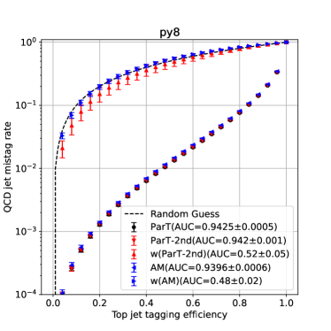
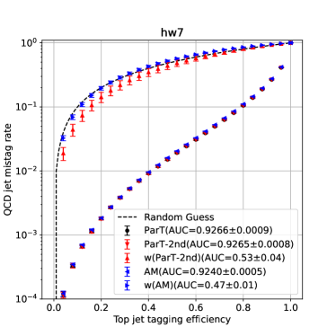
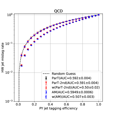
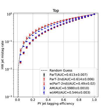
Figure 7: The average ROC curves and their standard deviations for the AM, ParT-best, and ParT-2nd trained on bootstrap datasets. Additionally, we show the ROC curves for the odds ratios $\mathrm{OR}^{\mathrm{I}/\mathrm{II}}$, where $\mathrm{I}$ is the ensemble average of ParT-best, and $\mathrm{II}$ is AM or ParT-2nd. The ROC curves shown here are for the following classification problems: (top left) $\mathrm{P_{T}}$ vs. $\mathrm{P_{Q}}$, (top right) $\mathrm{H_{T}}$ vs. $\mathrm{H_{Q}}$, (bottom left) $\mathrm{P_{Q}}$ vs. $\mathrm{H_{Q}}$, and (bottom right) $\mathrm{P_{T}}$ vs. $\mathrm{H_{T}}$.

Finally, Figure 7 shows the average and standard deviations of the ROC curves for the following classifiers trained on the bootstrap datasets: ParT-best (black circle), ParT-2nd (red inverted triangle), and AM (blue left-facing triangle). Additionally, we show the ROC curves from the odds ratio analysis Eq. 25 and Eq. 26 of ParT-best vs. ParT-2nd (in red triangles) and ParT-best against AM (in blue right-facing triangles). The ROC curves of AM are compatible with that of ParT within $3\sigma$, consistent with other metrics discussed previously. The ROC curves in the odds ratio analysis between ParT-best and AM look closer to the random guess, except for the classification ($\mathrm{P_{T}}$ vs. $\mathrm{H_{T}}$). But again, comparing the difference to the uncertainties of the odds ratio between ParT-best and Part-2nd, the gap becomes less significant. In summary, our AM is aligned to ParT sufficiently well for the top jet tagging and distinguishing simulations while showing smaller training uncertainties.

5 Summary and Conclusion

This paper introduces an analysis model (AM) employing the important high-level features (HLFs) in top jet tagging. The AM simplifies the current state-of-the-art taggers analyzing low-level features (LLFs) while maintaining classification performance. To demonstrate the effectiveness of our model, we revisited the problem of top jet tagging using various Monte Carlo simulated samples at the angular resolution of a hadronic calorimeter scale. We compared the classification performance of AM with a classifier based on the Particle Transformer (ParT). In our previous works, we have developed AMs using the IRC-safe relation network Lim:2018toa ; Chakraborty:2019imr ; Chakraborty:2020yfc and mathematical morphology for jet physics Chakraborty:2020yfc ; Lim:2020igi . This model’s performance matched the performance of a convolutional neural network, but it fell short of matching ParT’s performance. Nevertheless, once we fully considered the newly introduced features – $p_{T}$/̄conditioned jet constituent multiplicity distribution and subjet constituent multiplicities for capturing color charges of subjets – the performance of AM is aligned with that of ParT within a range of $2\sim 3\sigma$ of training uncertainties.

The compatibility between our AM and ParT varies depending on the specific classification problem. For instance, in the top tagging problem using Herwig-generated samples, AM demonstrates comparable performance to that of ParT. Similarly, AM matches ParT’s performance in distinguishing Pythia-generated QCD jets and Herwig-generated QCD jets. In the top tagging problem with Pythia-generated samples and distinguishing Pythia-generated top jets and Herwig-generated top jets, we observed discrepancies at the level of $2\sim 3\sigma$ of training uncertainty. The results suggest that Pythia-simulated jets may have unique features that are not covered by AM, and those are absent in Herwig-simulated jets. Identifying the HLFs exclusive to Pythia to fill this minor gap would be interesting, particularly in understanding the differences between simulations and calibrating those with experimental data; we plan to explore this in future studies.

One key advantage of employing simpler classifiers is the reduction in training uncertainty, a direct consequence of the bias-variance tradeoff. We explicitly demonstrated this behavior in AM through bootstrap methods applied to our jet tagging problems, and our AM demonstrated much smaller training uncertainty than ParT. Importantly, the smaller uncertainty is useful when classifiers are utilized for estimating statistical quantities, such as a likelihood ratio for reweighting simulated datasets nextpaper and decorrelating certain features by planing Chang:2017kvc ; deOliveira:2015xxd . We expect that our AM and this kind of HLF-analyzing classifier-based approach will be valuable in narrowing down uncertainties of reweighting-based calibration for simulated events Andreassen:2019nnm ; Gambhir:2022dut and synthetic samples from machine-learned generative models Diefenbacher:2020rna ; Butter:2021csz ; Das:2023ktd .

Appendix A Classification Results Involving Vincia Simulations

In this appendix, we present the classification results using samples generated Vincia (VIN). We remind that VIN-simulated top jet datasets and QCD jet datasets are denoted by $\mathrm{V_{T}}$ and $\mathrm{V_{Q}}$, respectively. Again, we focus on the following two types of classification problems: The first problem is top jet tagging trained on VIN-generated samples ($\mathrm{V_{T}}$ vs. $\mathrm{V_{Q}}$). The second problem is comparing VIN-simulated jets with jets from other simulations, specifically comparing PY and VIN (($\mathrm{P_{Q}}$ vs. $\mathrm{V_{Q}}$) and ($\mathrm{P_{T}}$ vs. $\mathrm{V_{T}}$)), and comparing VIN and HW (($\mathrm{V_{Q}}$ vs. $\mathrm{H_{Q}}$) and ($\mathrm{V_{T}}$ vs. $\mathrm{H_{T}}$)). We do not perform bootstrap analysis in this appendix; however, we expect that the training uncertainties will be similar to those of the corresponding problem in the main text, given that the same AM and ParT are used.

The classification performance metrics are shown in Table 7, Table 8, and Table 9. We show the naive statistical uncertainty estimations in the brackets. The difference in the classification performances between AM and ParT is negligible, mostly falling within the total training uncertainty. For the top jet simulation comparisons, some deviation is observed considering the statistical uncertainty. However, the total training uncertainty is about 5 to 10 times larger considering Table 4, and hence, the difference is not significant.

One notable observation is that the AUCs of top taggers trained on VIN-generated samples are larger than those of top taggers trained on PY-generated samples or HW-generated samples, shown in Table 2. This suggests that the systematical uncertainties from event generators remain substantial. The difference may be due to Vincia’s different treatment of initial and final state radiations Ritzmann:2012ca ; Fischer:2016vfv . However, a detailed discussion of this difference falls beyond the scope of the paper.

Finally, we compare the information content in the AM and ParT for VIN-involved classification problems, using the odds ratio $\mathrm{OR}^{\mathrm{I}/\mathrm{II}}$. The classification performance metrics for $\mathrm{OR}^{\mathrm{I}/\mathrm{II}}$ are shown in Table 10. Once again, the AUCs and rejection rates $R_{X\%}$ are close to no difference results, considering the large uncertainties associated with ParT, as shown in Table 6.

Model	$\mathrm{V_{T}}$ vs. $\mathrm{V_{Q}}$	$\mathrm{P_{Q}}$ vs. $\mathrm{V_{Q}}$	$\mathrm{V_{Q}}$ vs. $\mathrm{H_{Q}}$	$\mathrm{P_{T}}$ vs. $\mathrm{V_{T}}$	$\mathrm{V_{T}}$ vs. $\mathrm{H_{T}}$
ParT-best (as $\mathrm{I}$)	0.959	0.623	0.652	0.604	0.658
ParT-2nd (as $\mathrm{II}$)	0.959	0.623	0.651	0.602	0.658
AM (as $\mathrm{II}$)	0.960	0.623	0.650	0.610	0.651

Table 7: AUC of the AM and ParT in classifications involving VIN-generated datasets $\mathrm{V_{T}}$ and $\mathrm{V_{Q}}$. The best result for each classification problem is highlighted in boldface. However, the differences in AUC values between AM and ParT are not statistically significant.

Model	$\mathrm{V_{T}}$ vs. $\mathrm{V_{Q}}$	$\mathrm{P_{Q}}$ vs. $\mathrm{V_{Q}}$	$\mathrm{V_{Q}}$ vs. $\mathrm{H_{Q}}$	$\mathrm{P_{T}}$ vs. $\mathrm{V_{T}}$	$\mathrm{V_{T}}$ vs. $\mathrm{H_{T}}$
ParT-best (as $\mathrm{I}$)	186$(\pm 4)$	3.08$(\pm 0.01)$	3.43$(\pm 0.01)$	2.77$(\pm 0.01)$	3.53$(\pm 0.01)$
ParT-2nd (as $\mathrm{II}$)	184$(\pm 4)$	3.08$(\pm 0.01)$	3.41$(\pm 0.01)$	2.76$(\pm 0.01)$	3.52$(\pm 0.01)$
AM (as $\mathrm{II}$)	192$(\pm 4)$	3.07$(\pm 0.01)$	3.40$(\pm 0.01)$	2.84$(\pm 0.01)$	3.42$(\pm 0.01)$

Table 8: Rejection rate $R_{50\%}$ of the AM and ParT in classifications involving VIN-generated datasets $\mathrm{V_{T}}$ and $\mathrm{V_{Q}}$.

Model	$\mathrm{V_{T}}$ vs. $\mathrm{V_{Q}}$	$\mathrm{P_{Q}}$ vs. $\mathrm{V_{Q}}$	$\mathrm{V_{Q}}$ vs. $\mathrm{H_{Q}}$	$\mathrm{P_{T}}$ vs. $\mathrm{V_{T}}$	$\mathrm{V_{T}}$ vs. $\mathrm{H_{T}}$
ParT-best (as $\mathrm{I}$)	807$(\pm 40)$	6.20$(\pm 0.02)$	6.93$(\pm 0.03)$	5.30$(\pm 0.02)$	7.31$(\pm 0.03)$
ParT-2nd (as $\mathrm{II}$)	807$(\pm 40)$	6.20$(\pm 0.02)$	6.89$(\pm 0.03)$	5.26$(\pm 0.02)$	7.28$(\pm 0.03)$
AM (as $\mathrm{II}$)	835$(\pm 42)$	6.27$(\pm 0.03)$	6.84$(\pm 0.03)$	5.45$(\pm 0.02)$	7.03$(\pm 0.03)$

Table 9: Rejection rate $R_{30\%}$ of the AM and ParT in classifications involving VIN-generated datasets $\mathrm{V_{T}}$ and $\mathrm{V_{Q}}$.

$\mathrm{II}$	metric	$\mathrm{V_{T}}$ vs. $\mathrm{V_{Q}}$	$\mathrm{P_{Q}}$ vs. $\mathrm{V_{Q}}$	$\mathrm{V_{Q}}$ vs. $\mathrm{H_{Q}}$	$\mathrm{P_{T}}$ vs. $\mathrm{V_{T}}$	$\mathrm{V_{T}}$ vs. $\mathrm{H_{T}}$
ParT-2nd	AUC	0.5319	0.4965	0.4968	0.5043	0.4780
	$R_{50\%}$	2.25	1.99	1.97	2.02	1.88
	$R_{30\%}$	4.26	3.49	3.15	3.34	3.03
AM	AUC	0.5104	0.5214	0.5150	0.4901	0.5293
	$R_{50\%}$	2.09	2.15	2.09	1.95	2.17
	$R_{30\%}$	4.07	3.49	3.39	3.13	3.67

Table 10: Classification performance metrics for the odds ratio $\mathrm{OR}^{\mathrm{I}/\mathrm{II}}$, where $\mathrm{I}$ is ParT-best and $\mathrm{II}$ is AM and ParT-2nd. An AUC value closer to 0.5 and rejection rates $R_{X\%}$ closer to $1/X\%$ indicates that the two classifiers have similar information contents.

Appendix B Comparing Computational Resources utilized by AM and ParT

In this appendix, we describe the computation resources utilized by AM and ParT. During training with a batch size of 1,000, AM requires less than 1 GB of GPU memory, while ParT consumes approximately 14 GB. Additionally, the training process of AM is significantly faster. When training AM on an NVIDIA GeForce 1080 Ti GPU (FP32 performance: 11.3 TFLOPS), the training session takes 30 minute with an overall GPU utilization of 35%. In comparsion, training of ParT on an NVIDIA RTX 6000 GPU (FP32 performance: 38.7 TFLOPS) also takes 30 minutes, but with a GPU utilization of 95%. The ratio of the number of floating-point operations, calculated as (FP32 performance) $\times$ (GPU utilization) $\times$ (training time), between ParT and AM is approximately 18.3 to 2.0. This indicates that AM requires a significantly smaller number of GPU operations than ParT.

Appendix C Proof of Classifier Interpretation of Odds Ratio

In this appendix, we derive that $s^{\mathrm{I}/\mathrm{II}}$ is a classifier that relies solely on the features exclusive to the more expressive model. Let $\mathrm{I}$ be a more expressive model than $\mathrm{II}$ without loss of generality. We denote the common feature used in both $\mathrm{I}$ and $\mathrm{II}$ as $x_{2}$, and the exclusive feature as $x_{1}$. The classifier predictions $s^{\mathrm{I}}$ and $s^{\mathrm{II}}$ are regressing the posteriors for class 1,

$$s^{\mathrm{I}}(x_{1},x_{2})=p(y=1\,|\,x_{1},x_{2}),\quad s^{\mathrm{II}}(x_{2})=p(y=1\,|\,x_{2}).$$ (27)

The odds ratio is then written as a posterior odds ratio,

$$\mathrm{OR}^{\mathrm{I}/\mathrm{II}}(x_{1},x_{2})=\frac{p(y=1\,|\,x_{1},x_{2})}{p(y=0\,|\,x_{1},x_{2})}\cdot\frac{p(y=0\,|\,x_{2})}{p(y=1\,|\,x_{2})}.$$ (28)

By expanding the conditional probabilities, we can simplify the odds ratio to likelihood ratio between class labels given input $x_{1}$, conditioned on $x_{2}$,

$$\mathrm{OR}^{\mathrm{I}/\mathrm{II}}(x_{1},x_{2})=\frac{p(x_{1}\,|\,y=1,x_{2})}{p(x_{1}\,|\,y=0,x_{2})}.$$ (29)

From this point, let us regard $x_{2}$ in the above expression as a conditioning parameter of distribution rather than a random variable. We denote probability $p(\cdots,x_{2})$ conditioned on $x_{2}$ as $p_{x_{2}}(\cdots)$. The function $s^{\mathrm{I}/\mathrm{II}}$ is then written as follows:

$$s^{\mathrm{I}/\mathrm{II}}(x_{1},x_{2})=\frac{\mathrm{OR}^{\mathrm{I}/\mathrm{II}}(x_{1},x_{2})}{1+\mathrm{OR}^{\mathrm{I}/\mathrm{II}}(x_{1},x_{2})}=\frac{p_{x_{2}}(x_{1}\,|\,y=1)}{p_{x_{2}}(x_{1}\,|\,y=1)+p_{x_{2}}(x_{1}\,|\,y=0)}$$ (30)

The expression on the right-hand side is the posterior probability $p_{x_{2}}(y=1|x_{1})$ with a class prior $p_{x_{2}}(y)=0.5$. Therefore, $s^{\mathrm{I}/\mathrm{II}}$ can be interpreted as a classifier using only the exclusive feature $x_{1}$, given a fixed common feature $x_{2}$.

References

- (1) J. Cogan, M. Kagan, E. Strauss, and A. Schwarztman, Jet-Images: Computer Vision Inspired Techniques for Jet Tagging, JHEP 02 (2015) 118, [arXiv:1407.5675].
- (2) L. G. Almeida, M. Backović, M. Cliche, S. J. Lee, and M. Perelstein, Playing Tag with ANN: Boosted Top Identification with Pattern Recognition, JHEP 07 (2015) 086, [arXiv:1501.05968].
- (3) L. de Oliveira, M. Kagan, L. Mackey, B. Nachman, and A. Schwartzman, Jet-images — deep learning edition, JHEP 07 (2016) 069, [arXiv:1511.05190].
- (4) P. T. Komiske, E. M. Metodiev, and M. D. Schwartz, Deep learning in color: towards automated quark/gluon jet discrimination, JHEP 01 (2017) 110, [arXiv:1612.01551].
- (5) G. Kasieczka, T. Plehn, M. Russell, and T. Schell, Deep-learning Top Taggers or The End of QCD?, JHEP 05 (2017) 006, [arXiv:1701.08784].
- (6) S. Macaluso and D. Shih, Pulling Out All the Tops with Computer Vision and Deep Learning, JHEP 10 (2018) 121, [arXiv:1803.00107].
- (7) M. Farina, Y. Nakai, and D. Shih, Searching for New Physics with Deep Autoencoders, Phys. Rev. D 101 (2020), no. 7 075021, [arXiv:1808.08992].
- (8) J. Lin, M. Freytsis, I. Moult, and B. Nachman, Boosting with Machine Learning, JHEP 10 (2018) 101, [arXiv:1807.10768].
- (9) D. Guest, J. Collado, P. Baldi, S.-C. Hsu, G. Urban, and D. Whiteson, Jet Flavor Classification in High-Energy Physics with Deep Neural Networks, Phys. Rev. D 94 (2016), no. 11 112002, [arXiv:1607.08633].
- (10) G. Louppe, K. Cho, C. Becot, and K. Cranmer, QCD-Aware Recursive Neural Networks for Jet Physics, JHEP 01 (2019) 057, [arXiv:1702.00748].
- (11) T. Cheng, Recursive Neural Networks in Quark/Gluon Tagging, Comput. Softw. Big Sci. 2 (2018), no. 1 3, [arXiv:1711.02633].
- (12) J. M. Butterworth, A. R. Davison, M. Rubin, and G. P. Salam, Jet substructure as a new Higgs search channel at the LHC, Phys. Rev. Lett. 100 (2008) 242001, [arXiv:0802.2470].
- (13) D. E. Kaplan, K. Rehermann, M. D. Schwartz, and B. Tweedie, Top Tagging: A Method for Identifying Boosted Hadronically Decaying Top Quarks, Phys. Rev. Lett. 101 (2008) 142001, [arXiv:0806.0848].
- (14) T. Plehn, M. Spannowsky, M. Takeuchi, and D. Zerwas, Stop Reconstruction with Tagged Tops, JHEP 10 (2010) 078, [arXiv:1006.2833].
- (15) T. Plehn, M. Spannowsky, and M. Takeuchi, How to Improve Top Tagging, Phys. Rev. D 85 (2012) 034029, [arXiv:1111.5034].
- (16) J. Thaler and K. Van Tilburg, Identifying Boosted Objects with N-subjettiness, JHEP 03 (2011) 015, [arXiv:1011.2268].
- (17) J. Thaler and K. Van Tilburg, Maximizing Boosted Top Identification by Minimizing N-subjettiness, JHEP 02 (2012) 093, [arXiv:1108.2701].
- (18) A. J. Larkoski, G. P. Salam, and J. Thaler, Energy Correlation Functions for Jet Substructure, JHEP 06 (2013) 108, [arXiv:1305.0007].
- (19) A. J. Larkoski, I. Moult, and D. Neill, Power Counting to Better Jet Observables, JHEP 12 (2014) 009, [arXiv:1409.6298].
- (20) P. W. Battaglia, J. B. Hamrick, V. Bapst, A. Sanchez-Gonzalez, V. F. Zambaldi, M. Malinowski, A. Tacchetti, D. Raposo, A. Santoro, R. Faulkner, Ç. Gülçehre, H. F. Song, A. J. Ballard, J. Gilmer, G. E. Dahl, A. Vaswani, K. R. Allen, C. Nash, V. Langston, C. Dyer, N. Heess, D. Wierstra, P. Kohli, M. M. Botvinick, O. Vinyals, Y. Li, and R. Pascanu, Relational inductive biases, deep learning, and graph networks, arXiv:1806.01261.
- (21) A. Vaswani, N. Shazeer, N. Parmar, J. Uszkoreit, L. Jones, A. N. Gomez, L. u. Kaiser, and I. Polosukhin, Attention is all you need, in Advances in Neural Information Processing Systems (I. Guyon, U. V. Luxburg, S. Bengio, H. Wallach, R. Fergus, S. Vishwanathan, and R. Garnett, eds.), vol. 30, Curran Associates, Inc., 2017. arXiv:1706.03762.
- (22) H. Qu and L. Gouskos, ParticleNet: Jet Tagging via Particle Clouds, Phys. Rev. D 101 (2020), no. 5 056019, [arXiv:1902.08570].
- (23) Y. Wang, Y. Sun, Z. Liu, S. E. Sarma, M. M. Bronstein, and J. M. Solomon, Dynamic graph cnn for learning on point clouds, ACM Trans. Graph. 38 (oct, 2019) [arXiv:1801.07829].
- (24) P. T. Komiske, E. M. Metodiev, and J. Thaler, Energy Flow Networks: Deep Sets for Particle Jets, JHEP 01 (2019) 121, [arXiv:1810.05165].
- (25) M. Zaheer, S. Kottur, S. Ravanbakhsh, B. Poczos, R. R. Salakhutdinov, and A. J. Smola, Deep sets, in Advances in Neural Information Processing Systems (I. Guyon, U. V. Luxburg, S. Bengio, H. Wallach, R. Fergus, S. Vishwanathan, and R. Garnett, eds.), vol. 30, Curran Associates, Inc., 2017. arXiv:1703.06114.
- (26) A. Butter et al., The Machine Learning landscape of top taggers, SciPost Phys. 7 (2019) 014, [arXiv:1902.09914].
- (27) CMS Collaboration, Performance of heavy-flavour jet identification in boosted topologies in proton-proton collisions at , tech. rep., CERN, Geneva, 2023.
- (28) A. Chakraborty, S. H. Lim, M. M. Nojiri, and M. Takeuchi, Neural Network-based Top Tagger with Two-Point Energy Correlations and Geometry of Soft Emissions, JHEP 07 (2020) 111, [arXiv:2003.11787].
- (29) S. Gong, Q. Meng, J. Zhang, H. Qu, C. Li, S. Qian, W. Du, Z.-M. Ma, and T.-Y. Liu, An efficient Lorentz equivariant graph neural network for jet tagging, JHEP 07 (2022) 030, [arXiv:2201.08187].
- (30) A. Bogatskiy, T. Hoffman, D. W. Miller, and J. T. Offermann, PELICAN: Permutation Equivariant and Lorentz Invariant or Covariant Aggregator Network for Particle Physics, arXiv:2211.00454.
- (31) F. A. Dreyer, G. P. Salam, and G. Soyez, The Lund Jet Plane, JHEP 12 (2018) 064, [arXiv:1807.04758].
- (32) F. A. Dreyer and H. Qu, Jet tagging in the Lund plane with graph networks, JHEP 03 (2021) 052, [arXiv:2012.08526].
- (33) H. Qu, C. Li, and S. Qian, Particle Transformer for jet tagging, in Proceedings of the 39th International Conference on Machine Learning (K. Chaudhuri, S. Jegelka, L. Song, C. Szepesvari, G. Niu, and S. Sabato, eds.), vol. 162 of Proceedings of Machine Learning Research, pp. 18281–18292, PMLR, 17–23 Jul, 2022. arXiv:2202.03772.
- (34) A. Buckley et al., General-purpose event generators for LHC physics, Phys. Rept. 504 (2011) 145–233, [arXiv:1101.2599].
- (35) C. Bierlich et al., A comprehensive guide to the physics and usage of PYTHIA 8.3, arXiv:2203.11601.
- (36) J. Bellm et al., Herwig 7.0/Herwig++ 3.0 release note, Eur. Phys. J. C 76 (2016), no. 4 196, [arXiv:1512.01178].
- (37) Sherpa Collaboration, E. Bothmann et al., Event Generation with Sherpa 2.2, SciPost Phys. 7 (2019), no. 3 034, [arXiv:1905.09127].
- (38) J. Barnard, E. N. Dawe, M. J. Dolan, and N. Rajcic, Parton Shower Uncertainties in Jet Substructure Analyses with Deep Neural Networks, Phys. Rev. D 95 (2017), no. 1 014018, [arXiv:1609.00607].
- (39) A. Chakraborty, S. H. Lim, and M. M. Nojiri, Interpretable deep learning for two-prong jet classification with jet spectra, JHEP 07 (2019) 135, [arXiv:1904.02092].
- (40) S. H. Lim and M. M. Nojiri, Morphology for jet classification, Phys. Rev. D 105 (2022), no. 1 014004, [arXiv:2010.13469].
- (41) A. Ghosh and B. Nachman, A cautionary tale of decorrelating theory uncertainties, Eur. Phys. J. C 82 (2022), no. 1 46, [arXiv:2109.08159].
- (42) K. Cheung, Y.-L. Chung, S.-C. Hsu, and B. Nachman, Exploring the universality of hadronic jet classification, Eur. Phys. J. C 82 (2022), no. 12 1162, [arXiv:2204.03812].
- (43) P. T. Komiske, E. M. Metodiev, and J. Thaler, Energy flow polynomials: A complete linear basis for jet substructure, JHEP 04 (2018) 013, [arXiv:1712.07124].
- (44) R. Das, G. Kasieczka, and D. Shih, Feature Selection with Distance Correlation, arXiv:2212.00046.
- (45) S. H. Lim and M. M. Nojiri, Spectral Analysis of Jet Substructure with Neural Networks: Boosted Higgs Case, JHEP 10 (2018) 181, [arXiv:1807.03312].
- (46) M. Ritzmann, D. A. Kosower, and P. Skands, Antenna Showers with Hadronic Initial States, Phys. Lett. B 718 (2013) 1345–1350, [arXiv:1210.6345].
- (47) N. Fischer, S. Prestel, M. Ritzmann, and P. Skands, Vincia for Hadron Colliders, Eur. Phys. J. C 76 (2016), no. 11 589, [arXiv:1605.06142].
- (48) A. J. Larkoski, Binary Discrimination Through Next-to-Leading Order, arXiv:2309.14417.
- (49) J. Gallicchio and M. D. Schwartz, Seeing in Color: Jet Superstructure, Phys. Rev. Lett. 105 (2010) 022001, [arXiv:1001.5027].
- (50) J. Pumplin, Quark-gluon jet differences in decay, Phys. Rev. D 48 (1993) 1112–1116, [hep-ph/9301215].
- (51) L. Lee, C. Bell, J. Lawless, and E. Nibigira, QCD Reference Frames and False Jet Individualism, arXiv:2308.10951.
- (52) S. Catani, Y. L. Dokshitzer, M. H. Seymour, and B. R. Webber, Longitudinally invariant clustering algorithms for hadron hadron collisions, Nucl. Phys. B 406 (1993) 187–224.
- (53) S. D. Ellis and D. E. Soper, Successive combination jet algorithm for hadron collisions, Phys. Rev. D 48 (1993) 3160–3166, [hep-ph/9305266].
- (54) M. Cacciari, G. P. Salam, and G. Soyez, The anti- jet clustering algorithm, JHEP 04 (2008) 063, [arXiv:0802.1189].
- (55) F. V. Tkachov, Measuring multi - jet structure of hadronic energy flow or What is a jet?, Int. J. Mod. Phys. A12 (1997) 5411–5529, [hep-ph/9601308].
- (56) J. Gallicchio and M. D. Schwartz, Quark and Gluon Tagging at the LHC, Phys. Rev. Lett. 107 (2011) 172001, [arXiv:1106.3076].
- (57) D. Raposo, A. Santoro, D. G. T. Barrett, R. Pascanu, T. P. Lillicrap, and P. W. Battaglia, Discovering objects and their relations from entangled scene representations, CoRR abs/1702.05068 (2017) [arXiv:1702.05068].
- (58) A. Santoro, D. Raposo, D. G. Barrett, M. Malinowski, R. Pascanu, P. Battaglia, and T. Lillicrap, A simple neural network module for relational reasoning, in Advances in Neural Information Processing Systems 30 (I. Guyon, U. V. Luxburg, S. Bengio, H. Wallach, R. Fergus, S. Vishwanathan, and R. Garnett, eds.), pp. 4967–4976. Curran Associates, Inc., 2017. arXiv:1706.01427.
- (59) J. Pumplin, How to tell quark jets from gluon jets, Phys. Rev. D 44 (Oct, 1991) 2025–2032.
- (60) C. Frye, A. J. Larkoski, J. Thaler, and K. Zhou, Casimir Meets Poisson: Improved Quark/Gluon Discrimination with Counting Observables, JHEP 09 (2017) 083, [arXiv:1704.06266].
- (61) F. Chazal and B. Michel, An introduction to topological data analysis: Fundamental and practical aspects for data scientists, Frontiers in Artificial Intelligence 4 (2021) [arXiv:1710.04019].
- (62) S. Gillies, C. van der Wel, J. Van den Bossche, M. W. Taves, J. Arnott, B. C. Ward, and others, “Shapely.” https://github.com/shapely/shapely, Oct., 2023.
- (63) GEOS contributors, “GEOS coordinate transformation software library.” https://libgeos.org/, 2021.
- (64) Y. L. Dokshitzer, G. D. Leder, S. Moretti, and B. R. Webber, Better jet clustering algorithms, JHEP 08 (1997) 001, [hep-ph/9707323].
- (65) M. Wobisch and T. Wengler, Hadronization corrections to jet cross-sections in deep inelastic scattering, in Workshop on Monte Carlo Generators for HERA Physics (Plenary Starting Meeting), pp. 270–279, 4, 1998. hep-ph/9907280.
- (66) K. Datta and A. Larkoski, How Much Information is in a Jet?, JHEP 06 (2017) 073, [arXiv:1704.08249].
- (67) L. Moore, K. Nordström, S. Varma, and M. Fairbairn, Reports of My Demise Are Greatly Exaggerated: -subjettiness Taggers Take On Jet Images, SciPost Phys. 7 (2019), no. 3 036, [arXiv:1807.04769].
- (68) D. Athanasakos, A. J. Larkoski, J. Mulligan, M. Płoskoń, and F. Ringer, Is infrared-collinear safe information all you need for jet classification?, arXiv:2305.08979.
- (69) J. Alwall, R. Frederix, S. Frixione, V. Hirschi, F. Maltoni, O. Mattelaer, H. S. Shao, T. Stelzer, P. Torrielli, and M. Zaro, The automated computation of tree-level and next-to-leading order differential cross sections, and their matching to parton shower simulations, JHEP 07 (2014) 079, [arXiv:1405.0301].
- (70) P. Artoisenet, R. Frederix, O. Mattelaer, and R. Rietkerk, Automatic spin-entangled decays of heavy resonances in Monte Carlo simulations, JHEP 03 (2013) 015, [arXiv:1212.3460].
- (71) J. Bellm et al., Herwig 7.2 release note, Eur. Phys. J. C 80 (2020), no. 5 452, [arXiv:1912.06509].
- (72) P. Skands, S. Carrazza, and J. Rojo, Tuning PYTHIA 8.1: the Monash 2013 Tune, Eur. Phys. J. C 74 (2014), no. 8 3024, [arXiv:1404.5630].
- (73) DELPHES 3 Collaboration, J. de Favereau, C. Delaere, P. Demin, A. Giammanco, V. Lemaître, A. Mertens, and M. Selvaggi, DELPHES 3, A modular framework for fast simulation of a generic collider experiment, JHEP 02 (2014) 057, [arXiv:1307.6346].
- (74) A. De Roeck and H. Jung, eds., HERA and the LHC: A Workshop on the implications of HERA for LHC physics: Proceedings Part A, CERN Yellow Reports: Conference Proceedings, (Geneva), CERN, 12, 2005.
- (75) M. Cacciari, G. P. Salam, and G. Soyez, FastJet User Manual, Eur. Phys. J. C 72 (2012) 1896, [arXiv:1111.6097].
- (76) M. Cacciari and G. P. Salam, Dispelling the myth for the jet-finder, Phys. Lett. B 641 (2006) 57–61, [hep-ph/0512210].
- (77) G. Kasieczka, T. Plehn, J. Thompson, and M. Russel, “Top quark tagging reference dataset.” https://doi.org/10.5281/zenodo.2603256, Mar., 2019.
- (78) S. Shleifer, J. Weston, and M. Ott, Normformer: Improved transformer pretraining with extra normalization, arXiv:2110.09456.
- (79) H. Touvron, M. Cord, A. Sablayrolles, G. Synnaeve, and H. Jégou, Going deeper with image transformers, in Proceedings of the IEEE/CVF International Conference on Computer Vision (ICCV), pp. 32–42, October, 2021. arXiv:2103.17239.
- (80) A. Dosovitskiy, L. Beyer, A. Kolesnikov, D. Weissenborn, X. Zhai, T. Unterthiner, M. Dehghani, M. Minderer, G. Heigold, S. Gelly, J. Uszkoreit, and N. Houlsby, An image is worth 16x16 words: Transformers for image recognition at scale, in International Conference on Learning Representations, 2021. arXiv:2010.11929.
- (81) J. Devlin, M.-W. Chang, K. Lee, and K. Toutanova, Bert: Pre-training of deep bidirectional transformers for language understanding, arXiv:1810.04805.
- (82) M. Lin, Q. Chen, and S. Yan, Network in network, arXiv:1312.4400.
- (83) A. Furuichi, S. H. Lim, and M. M. Nojiri, in preparation, .
- (84) S. Chang, T. Cohen, and B. Ostdiek, What is the Machine Learning?, Phys. Rev. D 97 (2018), no. 5 056009, [arXiv:1709.10106].
- (85) A. Andreassen and B. Nachman, Neural Networks for Full Phase-space Reweighting and Parameter Tuning, Phys. Rev. D 101 (2020), no. 9 091901, [arXiv:1907.08209].
- (86) R. Gambhir, B. Nachman, and J. Thaler, Bias and priors in machine learning calibrations for high energy physics, Phys. Rev. D 106 (2022), no. 3 036011, [arXiv:2205.05084].
- (87) S. Diefenbacher, E. Eren, G. Kasieczka, A. Korol, B. Nachman, and D. Shih, DCTRGAN: Improving the Precision of Generative Models with Reweighting, JINST 15 (2020), no. 11 P11004, [arXiv:2009.03796].
- (88) A. Butter, T. Heimel, S. Hummerich, T. Krebs, T. Plehn, A. Rousselot, and S. Vent, Generative networks for precision enthusiasts, SciPost Phys. 14 (2023), no. 4 078, [arXiv:2110.13632].
- (89) R. Das, L. Favaro, T. Heimel, C. Krause, T. Plehn, and D. Shih, How to Understand Limitations of Generative Networks, arXiv:2305.16774.