Marginal phase transition in decorated single-chain Ising models

Abstract

Since Ernst Ising’s proof one century ago, it has been well-known that phase transition at finite temperature does not exist in the Ising model with short-range interactions in one dimension. Yet, little is known about whether this forbidden transition could be approached arbitrarily closely—at fixed finite temperature. To explore such asymptoticity, the notion of marginal phase transition (MPT) was introduced recently and spontaneous MPT was successfully found in decorated ladder Ising models. On the other hand, in the presence of a magnetic field, narrow phase crossover termed as pseudo-transition was found in decorated single-chain Ising models with strong geometric frustration; it is thus imperative to know whether the pseudo-transition could be transformed to approach a genuine transition at fixed finite temperature $T_{0}$ arbitrarily closely, i.e., being the MPT. Here, I reveal the existence of the field-induced MPT in decorated Ising chains, in which $T_{0}$ is determined by the interactions involving only the decorated parts and the magnetic field, while the crossover width $2\delta T$ is independently, exponentially reduced ($\delta T=0$ means a genuine transition) by the previously neglected ferromagnetic interaction between the ordinary spins on the chain backbone. Furthermore, I show that the MPT can be realized even in the decorated Ising chains without geometric frustration because the magnetic field itself can induce previously unnoticed hidden spin frustration. These findings manifest that MPT is essentially the buildup of coherence in preformed crossover of any local states, making the doors wide open to the engineering and utilization of MPT as a new paradigm for exploring exotic phenomena and 1D device applications.

The Ising model Ising1925 describes collective behaviors such as phase transitions and critical phenomena in various physical, biological, economical, and social systems Mattis_book_08_SMMS ; Mattis_book_1985 ; Baxter_book_Ising ; 003_Huang_08_book . The one-dimensional (1D) Ising model on a decorated single chain is generally defined as $H=H_{\mathrm{ordinary}}+\sum_{i}H^{(i)}_{\mathrm{decorated}}$, where

$$H_{\mathrm{ordinary}} = -J\sum_{i=1}^{N}\sigma_{i}\sigma_{i+1}-h\mu_{a}\sum_{i=1}^{N}\sigma_{i}$$ (1)

describes the ordinary single chain without the decoration (Fig. 1a) with $\sigma_{i}=\pm 1$ standing for the $i$th ordinary spin—in fact, it can be used to describe any two-value system, eg. open or close in neural networks Schneidman2006 , yes or no in voting. $N$ is the total number of the ordinary spins and $\sigma_{N+1}\equiv\sigma_{1}$ (i.e., the periodic boundary condition). $J$ is the interaction between nearest-neighboring ordinary spins. $h$ depicts the magnetic field and $\mu_{a}$ the magnetic moment of the ordinary spins. $H^{(i)}_{\mathrm{deorated}}$ describes the decorated part in between the $i$th and $(i+1)$th ordinary spins (Fig. 1b), which can be any finite-size subsystem as long as it couples to the two nearest ordinary spins by the Ising-type interactions only. To date, the simplest $H^{(i)}_{\mathrm{deorated}}$ considered in the literature of “pseudo-transition” 005_Galisova_PRE_15_double-tetrahedral-chain ; 007_Torrico_PRA_16_Ising-XYZ-diamond-chain ; 009_review_Souza_SSC_18_Ising-XYZ-diamond-chain_double-tetrahedral-chain-spin-electron ; 010_Carvalho_JMMM_18_Ising-XYZ-diamond-chain_quantum-entanglement ; 011_Rojas_BJP_20_Ising-Heisenberg-tetrahedral_diamond ; 013_Rojas_PRE_19_previous_4_models ; 014_Rojas_JPC_20_Ising–Heisenberg_spin-1-double-tetrahedral-chain ; 015_Strecka_APPA_20_Ising-diamond-chain ; 015-7_Canova_CzechoslovakJP_04_Ising–Heisenberg_diamond_chain ; 015-8_Canova_JPC_06_Ising–Heisenberg-spin-S-diamond-chain ; 017_Krokhmalskii_PA_21_3-previous-chains_effective_model ; 016_Strecka_book_chapter is the Ising diamond (Fig. 1d) given by 016_Strecka_book_chapter

$$H^{(i)}_{\mathrm{deorated}} = -J_{1}(\sigma_{i}+\sigma_{i+1})\sum_{k=1,2}s_{i,k}-J_{2}s_{i,1}s_{i,2}-h\mu_{b}\sum_{k=1,2}s_{i,k},$$ (2)

where $s_{i,k}=\pm 1$ denotes the $k$th decorated Ising spin for the $i$th bond of the ordinary chain or the backbone. $\mu_{b}$ is the magnetic moment of the decorated spins. The antiferromagnetic $J_{1}<0$ and $J_{2}<0$ were considered; they form triangles yielding strong geometric frustration Balents_nature_frustration ; Miyashita_10_review_frustration near $J_{2}/J_{1}=2$ 016_Strecka_book_chapter .

To search for MPT, which resembles a genuine first-order transition with large latent heat at fixed finite temperature $T_{0}$, in the decorated single-chain Ising models, it is instrumental to start with a comparative review of (i) the previous studies of the decorated Ising chains with pseudo-transition in the presence of magnetic field 005_Galisova_PRE_15_double-tetrahedral-chain ; 007_Torrico_PRA_16_Ising-XYZ-diamond-chain ; 009_review_Souza_SSC_18_Ising-XYZ-diamond-chain_double-tetrahedral-chain-spin-electron ; 010_Carvalho_JMMM_18_Ising-XYZ-diamond-chain_quantum-entanglement ; 011_Rojas_BJP_20_Ising-Heisenberg-tetrahedral_diamond ; 013_Rojas_PRE_19_previous_4_models ; 014_Rojas_JPC_20_Ising–Heisenberg_spin-1-double-tetrahedral-chain ; 015_Strecka_APPA_20_Ising-diamond-chain ; 015-7_Canova_CzechoslovakJP_04_Ising–Heisenberg_diamond_chain ; 015-8_Canova_JPC_06_Ising–Heisenberg-spin-S-diamond-chain ; 017_Krokhmalskii_PA_21_3-previous-chains_effective_model ; 016_Strecka_book_chapter and (ii) the recent investigations of the decorated Ising ladders with MPT in the absence of the magnetic field Yin_MPT ; Yin_icecreamcone ; Hutak_PLA_21_trimer . In particular, we ask questions as to what the pseudo-transition research has done and has not done, compared with what we have learned from the spontaneous MPT in the ladder. This task is greatly simplified by a recent summary 017_Krokhmalskii_PA_21_3-previous-chains_effective_model of the pseudo-transition research in the effective Hamiltonian approach, where tracing out the decorated parts results in the ordinary Ising-chain model with temperature-dependent parameters $J_{\mathrm{eff}}(T)$ and $h_{\mathrm{eff}}(T)$ in place of $J$ and $h$ in Eq. (1). Two key conclusions about the existence of the pseudo-transition were reached 017_Krokhmalskii_PA_21_3-previous-chains_effective_model : (1) $h_{\mathrm{eff}}(T)$ must experience the sign change as a function of temperature $T$ and $T_{0}$ is determined by $h_{\mathrm{eff}}(T)=0$. (2) The decoration was done to create geometrical frustration so that the system’s first low-lying excited state has much higher degeneracy and just slightly higher energy than the ground state, then an entropy-driven crossover between them would occur at finite temperature 005_Galisova_PRE_15_double-tetrahedral-chain ; 007_Torrico_PRA_16_Ising-XYZ-diamond-chain ; 009_review_Souza_SSC_18_Ising-XYZ-diamond-chain_double-tetrahedral-chain-spin-electron ; 010_Carvalho_JMMM_18_Ising-XYZ-diamond-chain_quantum-entanglement ; 011_Rojas_BJP_20_Ising-Heisenberg-tetrahedral_diamond ; 013_Rojas_PRE_19_previous_4_models ; 014_Rojas_JPC_20_Ising–Heisenberg_spin-1-double-tetrahedral-chain ; 015_Strecka_APPA_20_Ising-diamond-chain ; 015-7_Canova_CzechoslovakJP_04_Ising–Heisenberg_diamond_chain ; 015-8_Canova_JPC_06_Ising–Heisenberg-spin-S-diamond-chain ; 017_Krokhmalskii_PA_21_3-previous-chains_effective_model ; 016_Strecka_book_chapter . This physics of phase crossover is rather generic Miyashita_10_review_frustration ; what is challenging is how to make the crossover ultra-narrow. It was found that $T_{0}\to 0$ as the pseudo-transition is “tracked down in the critical point of the standard Ising-chain model at $h=0$ and $T=0$” 017_Krokhmalskii_PA_21_3-previous-chains_effective_model ; therefore, the pseudo-transition does not appear to support MPT at fixed finite $T_{0}$. The fact that spontaneous pseudo-transition in the decorated single-chain Ising models is prohibited by symmetry (namely the Ising model is invariant to the flipping of all the spins for $h=0$) motivated the discovery of the decorated Ising ladders as the paradigm for spontaneous MPT Yin_MPT ; Yin_icecreamcone . Now that the knowledge of MPT has become available, we understand that the following key pieces of information were missing in the previous studies of pseudo-transition and we are able to quickly find the solution:

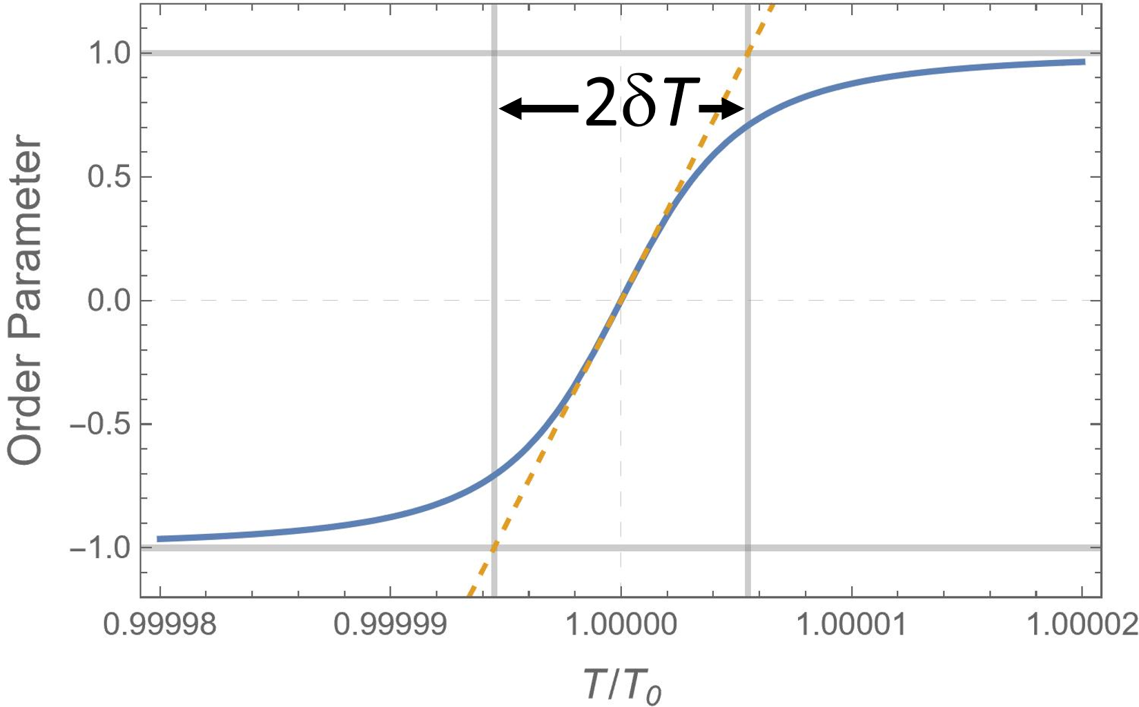
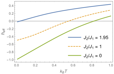
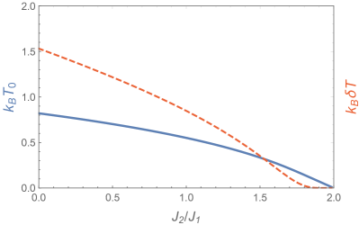
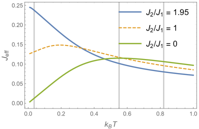
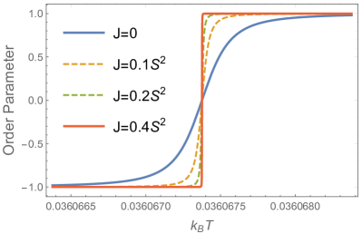
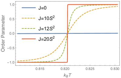
Figure 5: Order parameter $\langle\sigma_{i}\rangle$. (a) The definition of the crossover width $2\delta T=2\left(\partial\langle\sigma_{i}\rangle/\partial T\right)^{-1}_{T=T_{0}}$. The $T$ dependence of (b) $h_{\mathrm{eff}}$ and (d) $J_{\mathrm{eff}}$ for $J=0$ (light grey grid lines mark where $T_{0}$ is for $J_{2}/J_{1}=1.95,1,0$). (c) The $J_{2}/J_{1}$ dependence of $T_{0}$ (blue solid line; left axis) and $\delta T$ (red dashed line; right axis) for $J=0$. (e) The order parameter as a function of $T$ for $J_{2}/J_{2}=1.95$. (f) The order parameter as a function of $T$ for $J_{2}=0$. $J_{1}=-S^{2}$, $h=1$, and $\mu_{a}=\mu_{b}=S$ where $S=1/2$.

1) On the description of the targeted phenomenon.—The crossover width $2\delta T$ was never clearly defined and expressed by the model parameters (note that $\delta T=0$ means a genuine phase transition) for the pseudo-transition, while it was always presented in terms of specific heat, entropy, magnetic susceptibility, or overall magnetization 005_Galisova_PRE_15_double-tetrahedral-chain ; 007_Torrico_PRA_16_Ising-XYZ-diamond-chain ; 009_review_Souza_SSC_18_Ising-XYZ-diamond-chain_double-tetrahedral-chain-spin-electron ; 010_Carvalho_JMMM_18_Ising-XYZ-diamond-chain_quantum-entanglement ; 011_Rojas_BJP_20_Ising-Heisenberg-tetrahedral_diamond ; 013_Rojas_PRE_19_previous_4_models ; 014_Rojas_JPC_20_Ising–Heisenberg_spin-1-double-tetrahedral-chain ; 015_Strecka_APPA_20_Ising-diamond-chain ; 015-7_Canova_CzechoslovakJP_04_Ising–Heisenberg_diamond_chain ; 015-8_Canova_JPC_06_Ising–Heisenberg-spin-S-diamond-chain ; 017_Krokhmalskii_PA_21_3-previous-chains_effective_model ; 016_Strecka_book_chapter ; these physical quantities are derivatives of the free energy with respect to the global parameter $T$ or $h$ and thus depend on the details of the model. For spontaneous MPT in decorated Ising ladders, the on-rung parent-spin correlation function was identified as the order parameter (OP) that has a well-defined value space of $[-1,1]$ with the value $0$ meaning $T_{0}$ and its inverse slope at $T_{0}$ meaning $\delta T$, characterizing the MPT as an abrupt change in the OP between nearly $-1$ to nearly $+1$ Yin_MPT ; Yin_icecreamcone . Moreover, the general form of the OP does not depend on the details of the model; its mathematical derivation and numerical computation can be easily carried out. Such an OP provides an accurate, convenient, and microscopic description of the MPT; its identification greatly accelerated the search for MPT. Here for the decorated Ising chains, the OP that has the same features is $\langle\sigma_{i}\rangle$, the magnetization of the ordinary spins on the chain backbone (not the overall magnetization that includes the decorated parts): Its sign change and zero value at $T_{0}$ is consistent with the behavior of $h_{\mathrm{eff}}(T)$; its inverse derivative at $T_{0}$ defines $\delta T=\left(\partial\langle\sigma_{i}\rangle/\partial T\right)^{-1}_{T=T_{0}}$ (Fig. 5a).

2) On the model Hamiltonian.—Surprisingly, the $J$ term—the Ising interaction between the ordinary spins on the chain backbone (red bonds in Figs. 1a, 1b, 1e, 1f)—was neglected in the previous studies of pseudo-transition 005_Galisova_PRE_15_double-tetrahedral-chain ; 007_Torrico_PRA_16_Ising-XYZ-diamond-chain ; 009_review_Souza_SSC_18_Ising-XYZ-diamond-chain_double-tetrahedral-chain-spin-electron ; 010_Carvalho_JMMM_18_Ising-XYZ-diamond-chain_quantum-entanglement ; 011_Rojas_BJP_20_Ising-Heisenberg-tetrahedral_diamond ; 013_Rojas_PRE_19_previous_4_models ; 014_Rojas_JPC_20_Ising–Heisenberg_spin-1-double-tetrahedral-chain ; 015_Strecka_APPA_20_Ising-diamond-chain ; 015-7_Canova_CzechoslovakJP_04_Ising–Heisenberg_diamond_chain ; 015-8_Canova_JPC_06_Ising–Heisenberg-spin-S-diamond-chain ; 017_Krokhmalskii_PA_21_3-previous-chains_effective_model ; 016_Strecka_book_chapter , that is, Fig. 1c was studied instead of the more general Fig. 1b. A possible reason for the omission of $J$ could be that the standard geometric frustration from the triangles formed by the antiferromagnetic bonds is more obvious for $J=0$, as shown in Fig. 1d for the Ising diamond chain, the hitherto simplest model with pseudo-transition. However, the MPT for the Ising ladders tells us that the on-leg decoration (which controls $\delta T$) can be done independently of the on-rung decoration (which controls $T_{0}$) Yin_MPT ; Yin_icecreamcone . We shall use the $J\neq 0$ Ising diamond chain model (Fig. 1e) to show that similarly, the $J$ term independently exponentially reduces the crossover width $2\delta T$ for fixed finite $T_{0}$, since $J$ has no effect on $h_{\mathrm{eff}}(T)$ but is a separate addend in $J_{\mathrm{eff}}(T)$, i.e., $J_{\mathrm{eff}}(T,J)=J+J_{\mathrm{eff}}(T,0)$ (see Eq. (16) in the Method).

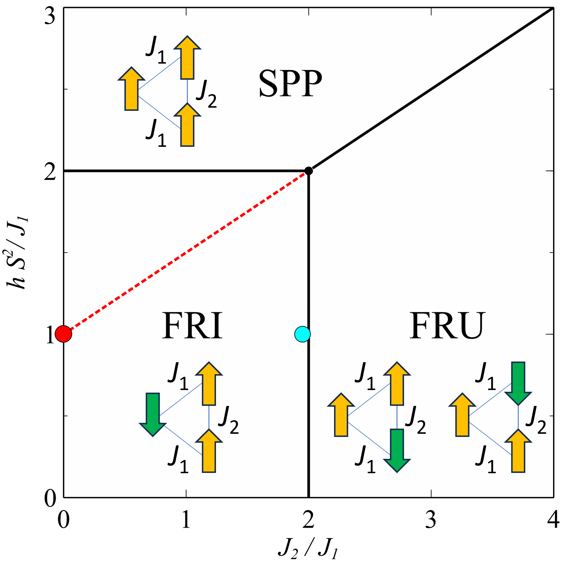
Figure 2: The ground-state phase diagram of the Ising diamond chain in the $J_{2}/J_{1}-h/J_{1}$ plane. Following Ref. 016_Strecka_book_chapter , we use the same notation for individual ground states to facilitate the comparison: FRI - the ferrimagnetic phase, FRU - the frustrated phase, SPP - the saturated paramagnetic phase. The focus of Ref. 016_Strecka_book_chapter was the case with strong geometric frustration (the cyan circle for $J_{2}/J_{1}=1.95$ near the FRI $-$ FRU boundary) as the FRU phase has the degeneracy of two per unit cell. Here we also study the case without geometric frustration (the red circle for $J_{2}=0$), which is located deep in the FRI phase, far away from the other two phases, but right on the extended line of the FRU $-$ SPP boundary (red dashed line) implying a hidden excited state with remarkably higher degeneracy than the FRI ground state. $J_{1}=-S^{2}$ and $\mu_{a}=\mu_{b}=S$ where $S=1/2$.

3) On the underlying mechanism.—Only the frustration of geometric frustration type (namely the lattice has frustration regardless of the magnetic field) was considered for the pseudo-transition. Using the effective Hamiltonian approach to study the same spontaneous MPT in the decorated Ising ladders with geometrically frustrated triangles as Refs. Yin_MPT ; Yin_icecreamcone , Hutak et al. conjectured that geometric frustration is not necessarily a prerequisite for the realization of spontaneous MPT in such ladders Hutak_PLA_21_trimer . Although this conjecture has not been proved for the ladder yet, we were inspired to extend the conjecture to the decorated single-chain Ising models, because it was recently emphasized Yin_g that the magnetic field on its own could induce hidden spin frustration in ferrimagnet-like systems without geometric frustration Bell_JPC_74_Ising_ferri_1 . It suffices to prove the conjecture with one example of the systems without geometric frustration; here we show that it is true in the Ising diamond chain for $J_{2}=0$ (Fig. 1f), where the triangles formed by the $J$ and $J_{1}$ bonds are not frustrated because $J>0$ is ferromagnetic. The hidden high degeneracy generated by the magnetic field, not by geometric frustration, is explained in the ground-state phase diagram of the Ising diamond chain (the red circle on the red dashed line in Fig. 2).

These findings thoroughly expose the mathematical structure of MPT in the 1D Ising models. One can use various decorations to yield even broad phase crossovers and then use interactions that enhance the coherence of the order parameter to turn the broad phase crossover to be the MPT, reminiscent of the notion of preformed pairs and their coherence buildup in the field of high-temperature superconductivity Emery_Nature_95 . Given the physical effects that the MPT resembles a genuine first-order phase transition with large latent heat and the fact that the Ising model has already been implemented in electronic circuits Ising_FPGA and optical networks Pierangeli_IsingMachine_PRL19 , the MPT-based 1D devices for thermal applications appear to be feasible. The features that $T_{0}$ and $2\delta T$ can be independently controlled by different parameters and different decoration methods could be attractive in engineering 1D thermal sensors, for example. The doors to the engineering and utilization of MPT are now wide open.

We describe the mathematical details in the Method section and show key results below. The OP is given by

$$\langle\sigma_{i}\rangle=\frac{\sinh(\beta h_{\mathrm{eff}}\mu_{a})}{\sqrt{\sinh^{2}(\beta h_{\mathrm{eff}}\mu_{a})+e^{-4\beta J_{\mathrm{eff}}}}}.$$ (3)

Clearly, $\langle\sigma_{i}\rangle\in[-1,1]$. $\langle\sigma_{i}\rangle=0$ when $h_{\mathrm{eff}}=0$ at $T_{0}$ and for fixed $T_{0}$, $\delta T\propto e^{-2J_{\mathrm{eff}}/k_{\mathrm{B}}T_{0}}$ exponentially decays as $J$, an addend in $J_{\mathrm{eff}}$, increases.

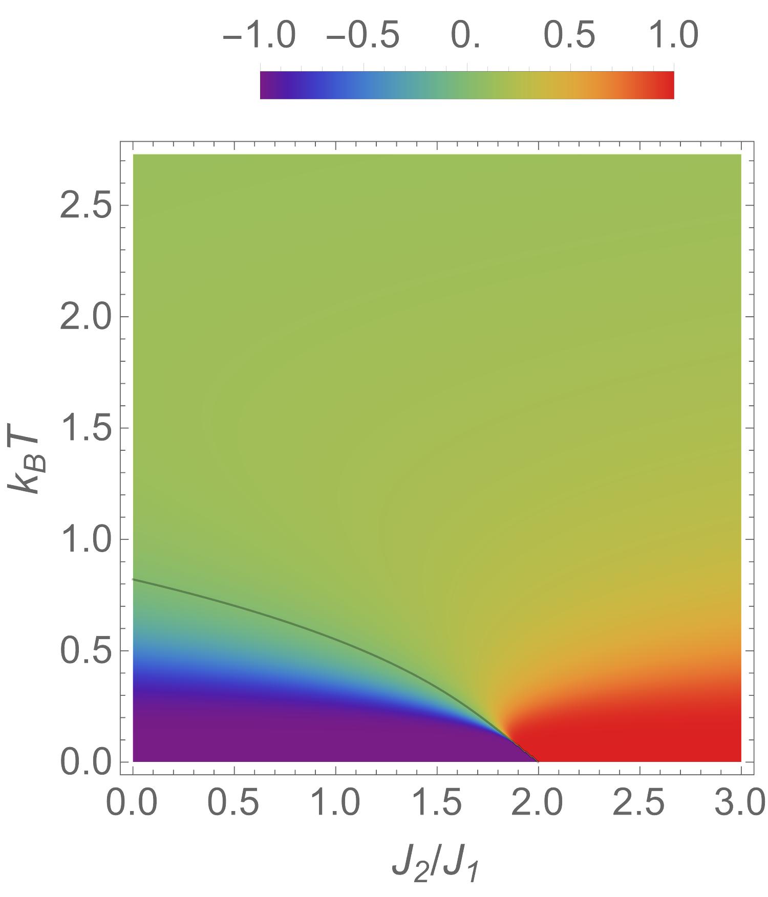
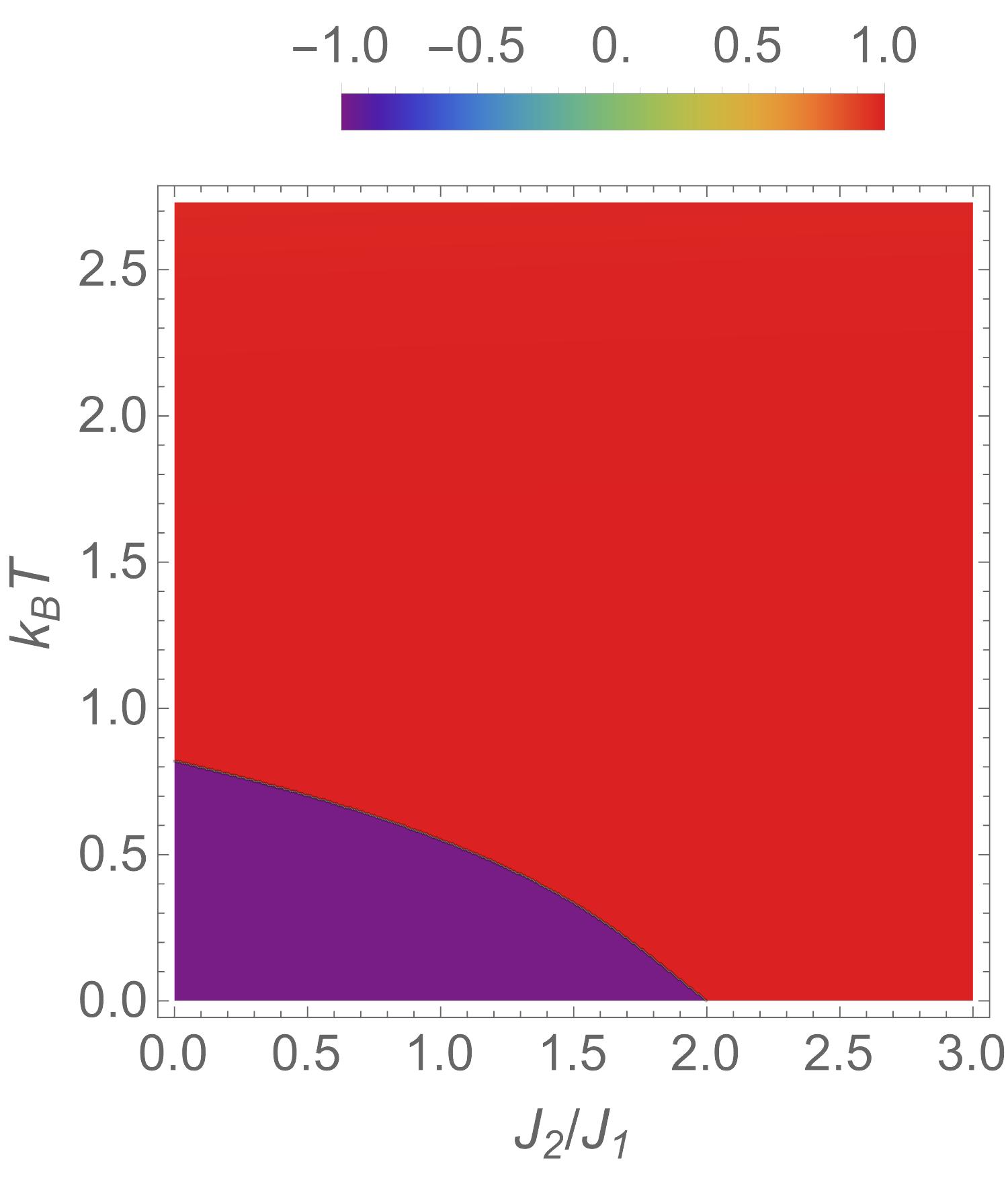
Figure 3: The $T-J_{2}$ Phase diagrams from the density plot of the order parameter $\langle\sigma_{i}\rangle$ for (a) $J=0$ and (b) $J=20S^{2}$. The black line is the phase boundary where $\langle\sigma_{i}\rangle=0$. $J_{1}=-S^{2}$, $h=1$, and $\mu_{a}=\mu_{b}=S$ where $S=1/2$.

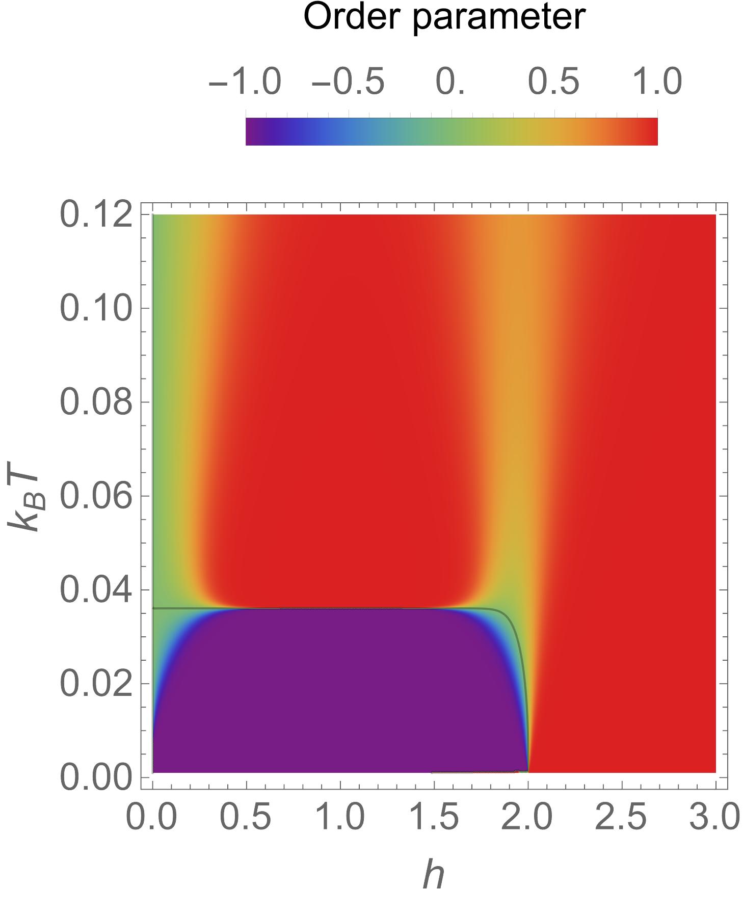
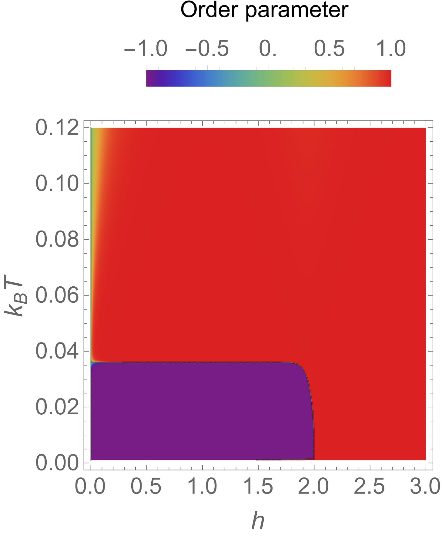
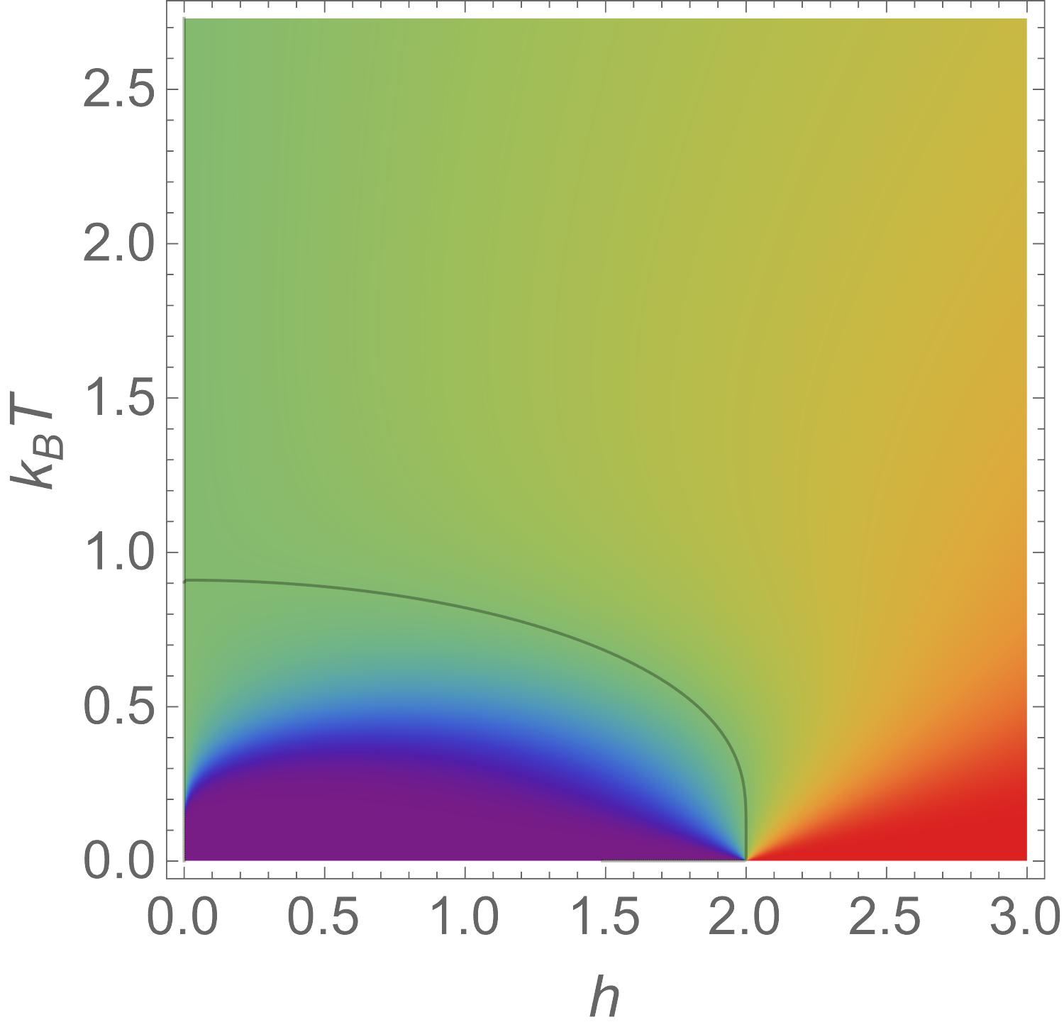
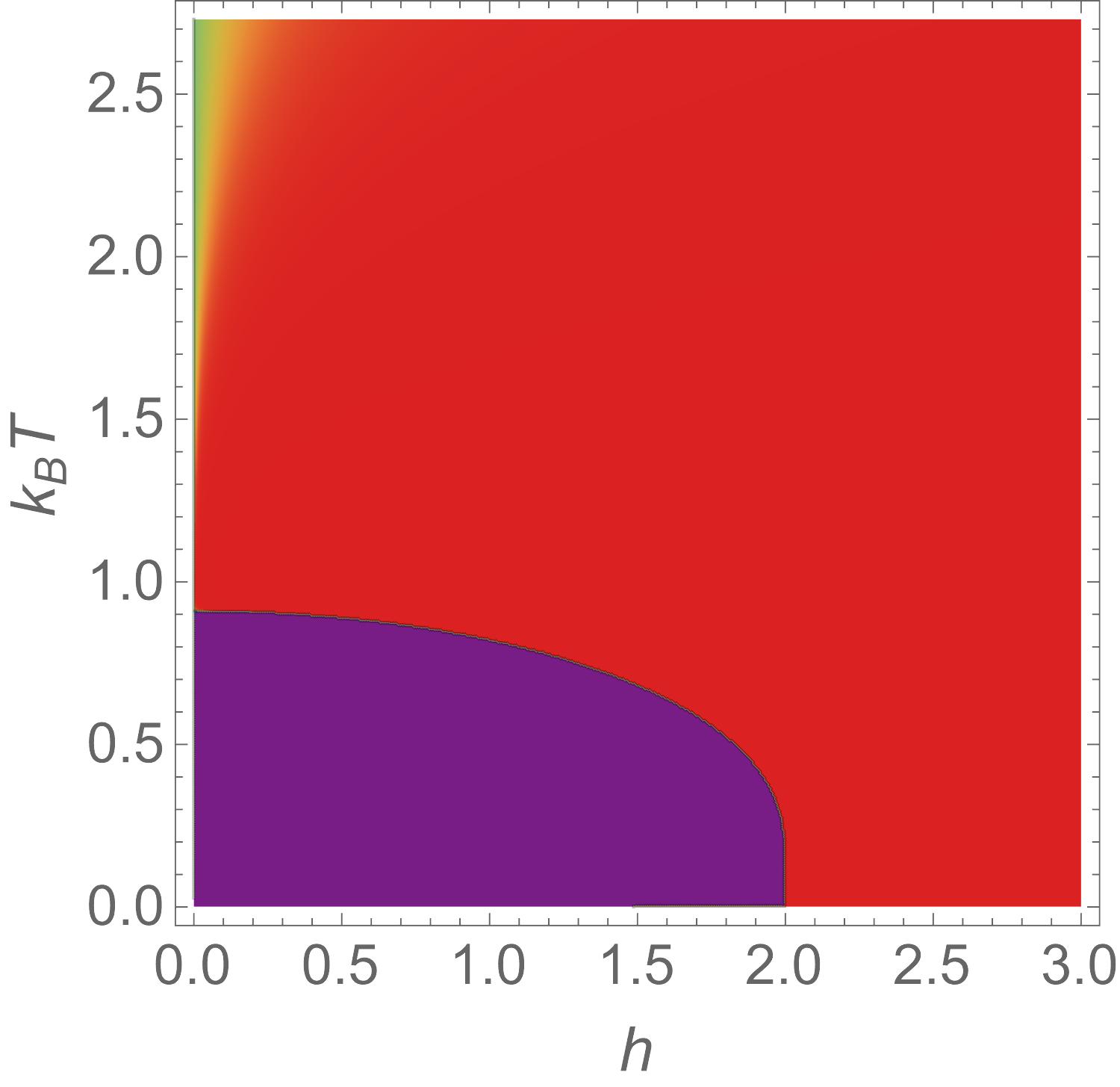
Figure 4: The $T-h$ Phase diagrams from the density plot of the order parameter $\langle\sigma_{i}\rangle$ for (a) $J_{2}/J_{1}=1.95$ and $J=0$, (b) $J_{2}/J_{1}=1.95$ and $J=0.4S^{2}$, (c) $J_{2}/J_{1}=0$ and $J=0$, (d) $J_{2}/J_{1}=0$ and $J=20S^{2}$. The black line is the phase boundary where $\langle\sigma_{i}\rangle=0$. $J_{1}=-S^{2}$ and $\mu_{a}=\mu_{b}=S$ where $S=1/2$.

The $T-J_{2}$ phase diagrams from the density plot of $\langle\sigma_{i}\rangle$ for the previously studied model (i.e., $J_{2}/J_{1}=1.95$ and $J=0$)  015_Strecka_APPA_20_Ising-diamond-chain ; 016_Strecka_book_chapter is presented in Fig. 3a. The sharp phase crossover from $\langle\sigma_{i}\rangle=-1$ to $+1$ occurs only near the small region with strong geometric frustration ($J_{2}/J_{1}=2$ is the FRI-FRU phase boundary; cf. Fig. 2). The resultant $T_{0}$ is very low ($k_{\mathrm{B}}T_{0}S^{2}/J_{1}\approx 0.036$ for $J_{2}/J_{1}=1.95$). As $J_{2}/J_{1}$ decreases, $T_{0}$ increases ($k_{\mathrm{B}}T_{0}S^{2}/J_{1}\approx 0.821$ for $J_{2}=0$) while the density is spread over a wider temperature interval, meaning larger $\delta T$. However, for the present new model with $J\neq 0$, Fig. 3b shows all the broad crossovers have been turned to be ultra-narrow MPT by increase $J$. The same is observed in the $T-h$ phase diagrams presented in Figs. 4a and 4b for $J_{2}/J_{1}=1.95$ and Figs. 4c and 4d for $J_{2}/J_{1}=0$.

To gain more insights, we present the $T$ dependence of $h_{\textrm{eff}}$ and $J_{\textrm{eff}}$ in Fig. 5b and 5d, respectively, for $J=0$ and several $J_{2}/J_{1}$, as well as $T_{0}$ and $\delta T$ as a function of $J_{2}/J_{1}$ in Fig. 5c. When $J=0$, $J_{\textrm{eff}}/k_{\mathrm{B}}T_{0}\approx 6.58$ for $J_{2}/J_{1}=1.95$ resulting in $\delta T\approx 2\times 10^{-7}$, but the value quickly drops to $J_{\textrm{eff}}/k_{\mathrm{B}}T_{0}\approx 0.13$ for $J_{2}=0$ resulting in $\delta T\approx 1.53$. Nevertheless, as we turn on $J$, $\delta T$ can be made narrower and narrower not only for the $J_{2}/J_{1}=1.95$ already ultra-narrow case (Fig. 5e) but also for the initially wide crossover for $J_{2}=0$ (Fig. 5f) with $T_{0}$ fixed in both cases. However, the underlying microscopic mechanisms for the former case with strong geometric frustration and the latter case without geometric frustration are quite different, as elaborated below.

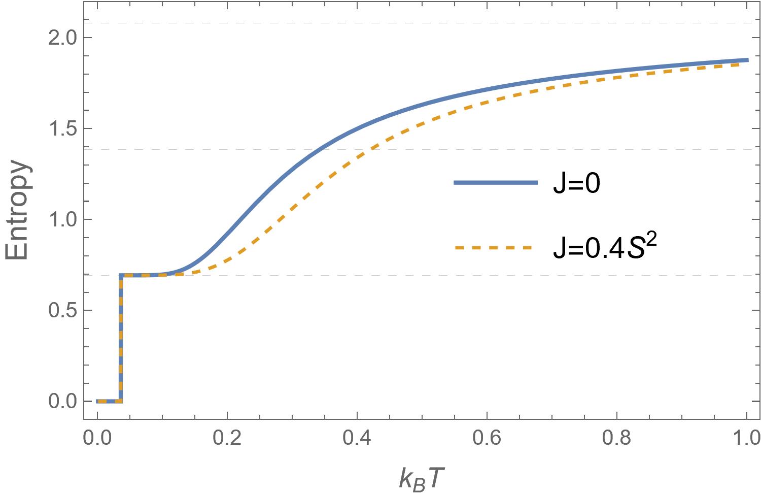
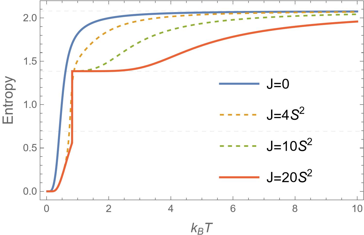
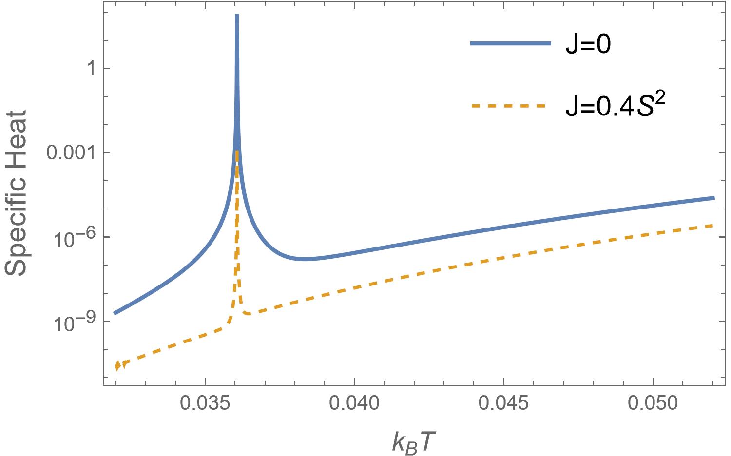
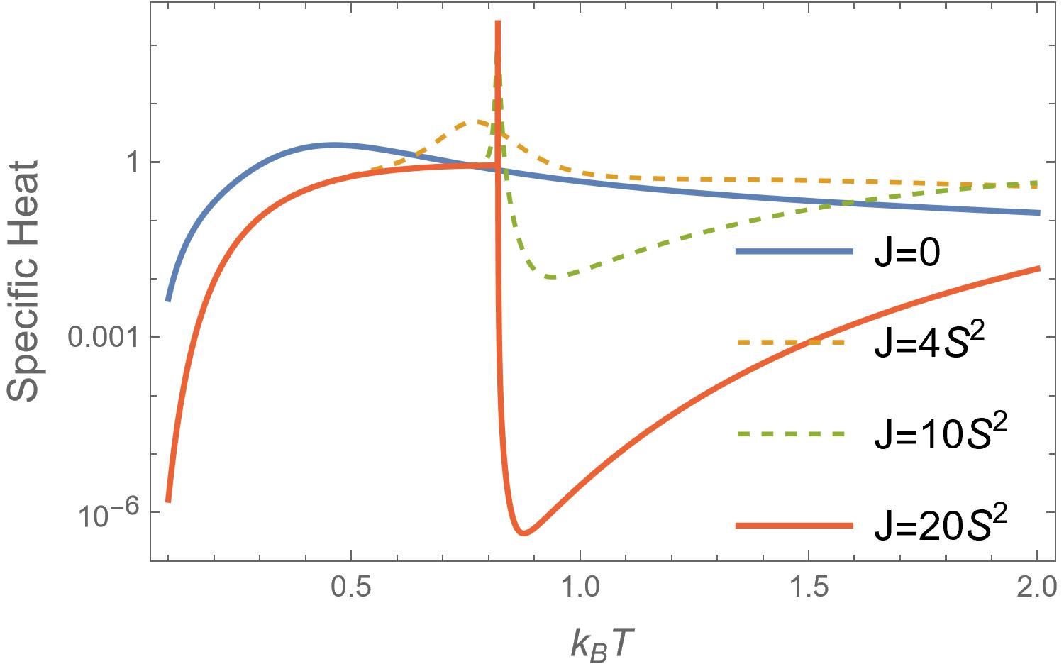
Figure 6: Thermodynamic properties. Entropy for (a) $J_{2}/J_{1}=1.95$ and (b) $J_{2}/J_{1}=0$, where the three light grey dashed lines denote the values of $\ln 2$, $2\ln 2$, and $3\ln 2$. Specific heat for (c) $J_{2}/J_{1}=1.95$ and (d) $J_{2}/J_{1}=0$. $J_{1}=-S^{2}$, $h=1$, and $\mu_{a}=\mu_{b}=S$ where $S=1/2$.

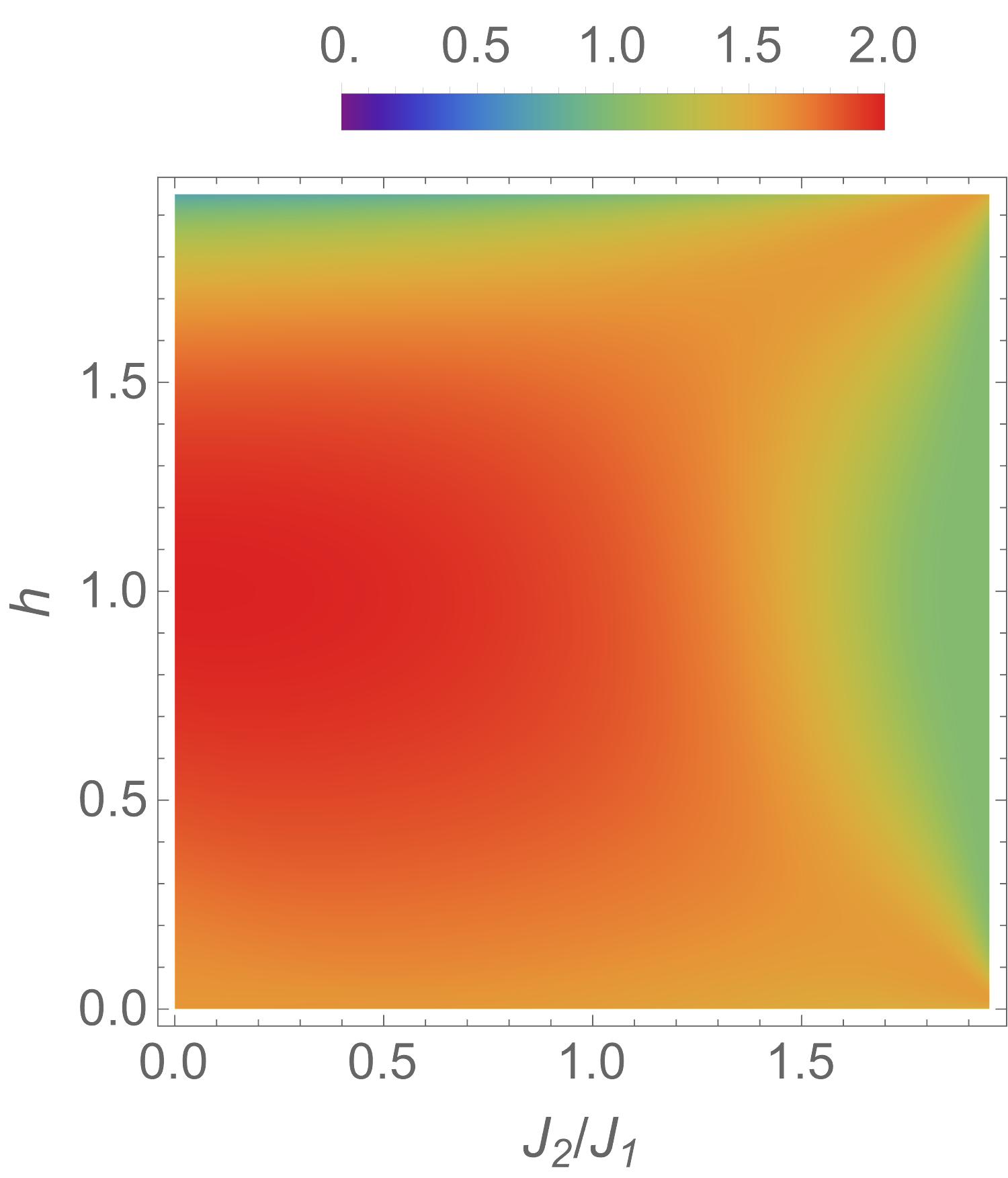
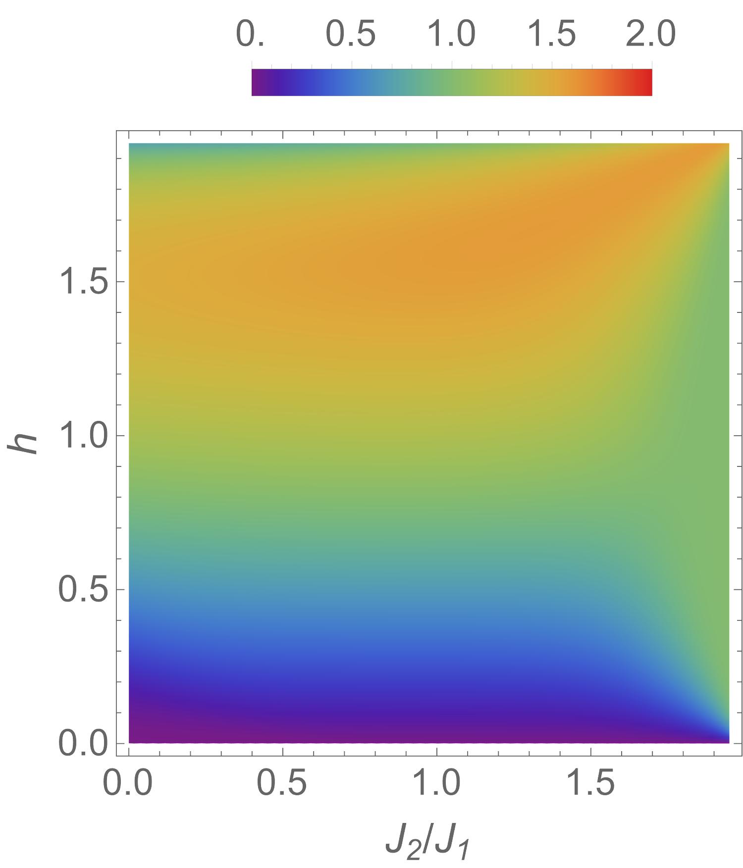
Figure 7: The $h-J_{2}$ density plots of (a) the entropy right above $T_{0}$ and (b) the entropy jump at $T_{0}$ in the unit of $\ln 2$ per unit cell. $J=20S^{2}$, $J_{1}=-S^{2}$, and $\mu_{a}=\mu_{b}=S$ where $S=1/2$.

As shown in Fig. 6, both cases resemble a genuine first-order phase transition with the entropy jump and gigantic susceptibility at $T_{0}$, but the entropy per unit cell is flattened at $\ln 2$ and $2\ln 2$ for $J_{2}/J_{1}=1.95$ (Fig. 6a) and $J_{2}=0$ (Fig. 6b), respectively. The former is expected since the case with $J_{2}/J_{1}=1.95$ is located near the FRI-FRU phase boundary in the ground-state phase diagram (the cyan circle in Fig. 2). The FRU phase has the degeneracy of two per unit cell due to the frustrated decorated spins; the crossover is driven by this entropy gain by $\ln 2$ per unit cell 016_Strecka_book_chapter , while the ordinary spins flip from $\sigma_{i}\approx-1$ to $+1$ still being locked together by large $J_{\mathrm{eff}}/k_{\mathrm{B}}T_{0}$. By sharp contrast, the case with $J_{2}=0$ is far away from any phase boundary and the entropy flattening at $2\ln 2$ is astonishing. This exotic phenomenon originates from a hidden remarkably high degeneracy induced by the magnetic field even in the system without geometric frustration: As shown by the red circle in Fig. 2, the case with $J_{2}=0$ is seated right on the extended line of the FRU-SPP phase boundary (red dashed line). This means that once the system is heated out of the FRI ground state, it will be frustrated in choosing between FRU or SPP, resulting in the effective decoupling of the two decorated spins per unit cell from the lattice—that is the entropy gain of $2\ln 2$. Meanwhile, the ordinary spins flip from $\sigma_{i}\approx-1$ to $+1$ and are still locked together by large $J_{\mathrm{eff}}/k_{\mathrm{B}}T_{0}$. In other words, it is this lockup, “calm,” or the buildup of coherence in the order parameter $\sigma_{i}$ of the ordinary spins that makes the decorated spins fully frustrated in response to the heated atmosphere. This is a distinctly new mechanism for driving the MPT. It is also opposite to the zero-temperature critical point recently emphasized as the “half-ice half-fire” state in ferrimagnet-like systems where the ordinary spins are fully frustrated while the decorated spins are forced to be calm by the critical magnetic field Yin_g . Now the FRI regime of the ground-state phase diagram has two paths toward MPT through either the geometric-frustration-driven FRI-FRU or the hidden-frustration-driven FRU-SPP phase boundary. As demonstrated in the density plot of the entropy right above $T_{0}$ (Fig. 7a) and that of the entropy jump at $T_{0}$ (Fig. 7b), the entropy jump of about $\ln 2$ to $2\ln 2$ takes place in most areas of the FRI regime except for weak $h$ and the largest jump occurs approximately along the hidden frustration line. This difference in the entropy jump together with $T_{0}$ and $\delta T$ could be used to train deep neural networks to predict the model parameters of the decorated 1D Ising model with MPT Yin_PRB_23_ML_t-J .

In summary, a simple and general way by including the ferromagnetic $J$ term is found to not only transform all the previously studied systems—with geometric frustration—in the context of pseudo-transition into the MPT cases, but also unexpectedly expose the hidden field-induced frustration to generate the MPT in decorated Ising chains without geometric frustration. With the discoveries of both the spontaneous MPT in the decorated Ising two-leg ladders (which is DNA-like) and the field-driven MPT in the decorated Ising single chains (which is RNA-like), the foundation of the MPT research direction has been solidly established. Given the prominent roles of the Ising model and frustration in understanding collective phenomena in various physical, biological, economical, and social systems, and the prominent roles of 1D systems in research, education, and technology applications, we anticipate that the present new insights to phase transitions and the dynamical actions of frustration will stimulate further research and development about MPT.

The Method

The central quantity of statistic mechanics is the partition function $Z=\mathrm{Tr}\left(e^{-\beta H}\right)$ where $H$ is the Hamiltonian of the system and $\beta=1/(k_{\mathrm{B}}T)$ with $T$ being the temperature and $k_{\mathrm{B}}$ the Boltzmann constant Mattis_book_08_SMMS . The free energy $f(T)=-k_{\mathrm{B}}T\ln Z$ determines many important thermodynamic properties such as the entropy $S=-\partial f/\partial T$, the specific heat $C_{v}=T\partial S/\partial T$, the magnetization $m=-\partial f/\partial h$, and the magnetic susceptibility $\chi=\partial m/\partial h$. Here the OP is $\langle\sigma_{i}\rangle=-(1/h)\partial f/\partial\mu_{a}$.

The partition function of a 1D Ising model can be obtained exactly by using the transfer matrix method Mattis_book_08_SMMS ; Mattis_book_1985 ; Baxter_book_Ising ; 003_Huang_08_book ; 005_Galisova_PRE_15_double-tetrahedral-chain ; 007_Torrico_PRA_16_Ising-XYZ-diamond-chain ; 009_review_Souza_SSC_18_Ising-XYZ-diamond-chain_double-tetrahedral-chain-spin-electron ; 010_Carvalho_JMMM_18_Ising-XYZ-diamond-chain_quantum-entanglement ; 011_Rojas_BJP_20_Ising-Heisenberg-tetrahedral_diamond ; 013_Rojas_PRE_19_previous_4_models ; 014_Rojas_JPC_20_Ising–Heisenberg_spin-1-double-tetrahedral-chain ; 015_Strecka_APPA_20_Ising-diamond-chain ; 015-7_Canova_CzechoslovakJP_04_Ising–Heisenberg_diamond_chain ; 015-8_Canova_JPC_06_Ising–Heisenberg-spin-S-diamond-chain ; 017_Krokhmalskii_PA_21_3-previous-chains_effective_model ; 016_Strecka_book_chapter ; Yin_MPT ; Yin_icecreamcone ; Hutak_PLA_21_trimer ; Yin_g ; Bell_JPC_74_Ising_ferri_1 and is given by

$$Z=\mathrm{Tr}\left(\Lambda^{N}\right)=\sum_{k}{\lambda_{k}^{N}}\;\;\to\;\;\lambda^{N}\;\mathrm{for}\;N\to\infty,$$ (4)

where $\Lambda$ is the transfer matrix, $\lambda_{k}$ the $k$th eigenvalue of $\Lambda$, and $\lambda$ the largest eigenvalue. Thus, in the thermodynamic limit, the free energy per unit cell $f(T)=-\lim_{N\to\infty}\frac{1}{N}k_{\mathrm{B}}T\ln Z=-k_{\mathrm{B}}T\ln\lambda$.

To calculate the partition function $Z=\mathrm{Tr}\left(e^{-\beta H}\right)$ for the general model of the decorated Ising chains defined in Eq. (1) and illustrated in Fig. 1b, the decorated sites can be exactly summed out as they are coupled only to the nearest neighboring ordinary spins, yielding the decoration’s contribution functions

$$\boxed{\pm\pm}_{i}=\sum\left(e^{\beta H^{(i)}_{\mathrm{decorated}}}\right)_{{\sigma_{i}=\pm 1},\;\sigma_{i+1}=\pm 1}$$ (5)

where the sum is over all possible states made up by the decorated subsystem for one of the four combinations of $(\sigma_{i}$, $\sigma_{i+1})=(\pm 1,\pm 1)$. They are translationally invariant, i.e., $\boxed{\pm\pm}_{i}=\boxed{\pm\pm}$.

The transfer matrix is of the following form:

$$\Lambda_{\mathrm{single-chain}}=\left(\begin{array}[]{cc}a&c\\ c&b\\ \end{array}\right)=\left(\begin{array}[]{cc}e^{\beta J+\beta h\mu_{a}}\boxed{++}&e^{-\beta J}\boxed{+-}\\ e^{-\beta J}\boxed{-+}&e^{\beta J-\beta h\mu_{a}}\boxed{--}\\ \end{array}\right),$$ (10)

Its largest eigenvalue is

$$\lambda=\frac{1}{2}e^{\beta J}\left[\Upsilon_{+}+\sqrt{\Upsilon_{-}^{2}+4e^{-4\beta J}\boxed{+-}^{2}}\right],$$ (11)

with the frustration functions

$$\Upsilon_{\pm} = e^{\beta\mu_{a}h}\boxed{++}\pm e^{-\beta\mu_{a}h}\boxed{--},$$ (12)

which is independent of $J$.

The crossing of $a$ and $b$ in Eq. (10) occurs when $\Upsilon_{-}$ changes sign at $T_{0}$ where $\Upsilon_{-}=0$. This means that $T_{0}$ is independent of $J$. Meanwhile, the $\boxed{+-}$ term in Eq. (11) has a prefactor of $e^{-4\beta J}$, which exponentially decreases to zero as ferromagnetic $J>0$ increases for fixed finite $T_{0}$; thus, if Eq. (11) is approximated by neglecting the $\boxed{+-}$ term inside $\sqrt{\cdots}$,

$$\lambda\simeq\frac{1}{2}e^{\beta J}(\Upsilon_{+}+|\Upsilon_{-}|),$$ (13)

which becomes non-analytic. The difference between Eq. (11) and Eq. (13) takes place in a region of $(T_{0}-\delta T,T_{0}+\delta T)$, where the crossover width $2\delta T$ can be estimated by $|\Upsilon_{-}|=2e^{-2\beta J}\boxed{+-}$ at $T_{0}\pm\delta T$. Following Ref. , an alternative and consistent way to measure $\delta T$ is to find such an order parameter that has a well-defined value space of $[-1,1]$ with the value $0$ meaning $T_{0}$ and its inverse slope at $T_{0}$ meaning $\delta T$. It is the magnetization of the ordinary spins given by

$$\langle\sigma_{i}\rangle=-\frac{\partial f}{\partial(h\mu_{a})}=\frac{\Upsilon_{-}}{\sqrt{\Upsilon_{-}^{2}+4e^{-4\beta J}\boxed{+-}^{2}}}.$$ (14)

$$\delta T=\left(\frac{\partial\langle\sigma_{i}\rangle}{\partial T}\right)^{-1}_{T=T_{0}}=e^{-\frac{2J}{k_{\mathrm{B}}T_{0}}}\frac{4k_{\mathrm{B}}T_{0}^{2}\boxed{+-}}{-\Upsilon_{+}}\left[2h\mu_{a}+\left(\frac{\partial\ln\boxed{++}}{\partial\beta}-\frac{\partial\ln\boxed{--}}{\partial\beta}\right)\right]^{-1}_{\beta=\frac{1}{k_{\mathrm{B}}T_{0}}}.$$ (15)

Again, it is clear that the crossover width $2\delta T$ decreases exponentially as $J$ increases for fixed finite $T_{0}$. This order parameter provides an accurate, convenient, and microscopic description of MPT. The use of the MPT order parameter accelerates the finding of MPT.

The above exact solution can also be represented in terms of temperature-dependent effective interactions and field on the ordinary spins 017_Krokhmalskii_PA_21_3-previous-chains_effective_model ; Yin_MPT ; Yin_icecreamcone ; Hutak_PLA_21_trimer :

$$h_{\mathrm{eff}} = \frac{1}{2\beta\mu_{a}}(\ln a-\ln b)=h+\frac{1}{2\beta\mu_{a}}\left(\ln\boxed{++}-\ln\boxed{--}\right),$$ (16)

$$J_{\mathrm{eff}} = \frac{1}{2\beta}\left[\frac{1}{2}(\ln a+\ln b)-\ln c\right]=J+\frac{1}{2\beta}\left[\frac{1}{2}\left(\ln\boxed{++}+\ln\boxed{--}\right)-\ln\boxed{+-}\right],$$

$$A = \frac{1}{2\beta}\left[\frac{1}{2}(\ln a+\ln b)+\ln c\right]=\frac{1}{2\beta}\left[\frac{1}{2}\left(\ln\boxed{++}+\ln\boxed{--}\right)+\ln\boxed{+-}\right].$$

Note that $\mu_{a}$ appears in $h_{\mathrm{eff}}$ only and $J$ appears in $J_{\mathrm{eff}}$ only—with $J_{\mathrm{eff}}(T,J)=J+J_{\mathrm{eff}}(T,0)$. This means that $J$ has no impact on the determination of $T_{0}$, therefore it can be used to change $\delta T$ for fixed $T_{0}$. The resulting transfer matrix is expressed by

$$\Lambda_{\mathrm{single-chain}}=\left(\begin{array}[]{cc}a&c\\ c&b\\ \end{array}\right)=e^{\beta A}\left(\begin{array}[]{cc}e^{\beta J_{\mathrm{eff}}+\beta h_{\mathrm{eff}}\mu_{a}}&e^{-\beta J_{\mathrm{eff}}}\\ e^{-\beta J_{\mathrm{eff}}}&e^{\beta J_{\mathrm{eff}}-\beta h_{\mathrm{eff}}\mu_{a}}\\ \end{array}\right),$$ (21)

Its largest eigenvalue is

$$\lambda=e^{\beta A}e^{\beta J_{\mathrm{eff}}}\left[\cosh(\beta h_{\mathrm{eff}}\mu_{a})+\sqrt{\sinh^{2}(\beta h_{\mathrm{eff}}\mu_{a})+e^{-4\beta J_{\mathrm{eff}}}}\right].$$ (22)

$T_{0}$ is determined by $\sinh(\beta h_{\mathrm{eff}}\mu_{a})=0$, i.e., $h_{\mathrm{eff}}(T_{0})=0$ 017_Krokhmalskii_PA_21_3-previous-chains_effective_model , which is the same as $\Upsilon_{-}(T_{0})=0$. The order parameter is

$$\langle\sigma_{i}\rangle=-\frac{\partial f}{\partial(h\mu_{a})}=-\frac{\partial f}{\partial(h_{\mathrm{eff}}\mu_{a})}=\frac{\sinh(\beta h_{\mathrm{eff}}\mu_{a})}{\sqrt{\sinh^{2}(\beta h_{\mathrm{eff}}\mu_{a})+e^{-4\beta J_{\mathrm{eff}}}}}.$$ (23)

$$\delta T=\left(\frac{\partial\langle\sigma_{i}\rangle}{\partial T}\right)^{-1}_{T=T_{0}}=e^{-\frac{2J_{\mathrm{eff}}}{k_{\mathrm{B}}T_{0}}}\frac{k_{\mathrm{B}}T_{0}^{2}}{-\cosh(\beta h_{\mathrm{eff}}\mu_{a})}\left[h_{\mathrm{eff}}\mu_{a}+\beta\mu_{a}\left(\frac{\partial h_{\mathrm{eff}}}{\partial\beta}\right)\right]^{-1}_{\beta=\frac{1}{k_{\mathrm{B}}T_{0}}}.$$ (24)

Eq. (23) and Eq. (24) are the same as Eq. (14) and Eq. (15), respectively. These two different representations can be used to verify the results obtained from using the other method.

For the Ising diamond chain model defined in Eq. (2) and illustrated in Fig. 1e,

$${\boxed{++}} = 2\cosh(4\beta J_{1}+2\beta h\mu_{b})e^{\beta J_{2}}+2e^{-\beta J_{2}},$$

$${\boxed{--}} = 2\cosh(4\beta J_{1}-2\beta h\mu_{b})e^{\beta J_{2}}+2e^{-\beta J_{2}},$$ (25)

$${\boxed{+-}} = {\boxed{-+}}=2\cosh(2\beta h\mu_{b})e^{\beta J_{2}}+2e^{-\beta J_{2}}.$$

For $J_{2}=0$, the Ising diamond chain does not have geometric frustration, as shown in Fig. 1f,

$${\boxed{++}} = [2\cosh(2\beta J_{1}+\beta h\mu_{b})]^{2},$$

$${\boxed{--}} = [2\cosh(2\beta J_{1}-\beta h\mu_{b})]^{2},$$ (26)

$${\boxed{+-}} = {\boxed{-+}}=[2\cosh(\beta h\mu_{b})]^{2}.$$

$$\begin{split}\delta T=e^{-\frac{2J}{k_{\mathrm{B}}T_{0}}}\frac{2k_{\mathrm{B}}T_{0}^{2}\boxed{+-}}{-\Upsilon_{+}}\biggl{[}h\mu_{a}&+(2\beta J_{1}+\beta h\mu_{b})\tanh(2\beta J_{1}+\beta h\mu_{b})\\ &+(2\beta J_{1}-\beta h\mu_{b})\tanh(2\beta J_{1}-\beta h\mu_{b})\biggr{]}^{-1}_{\beta=\frac{1}{k_{\mathrm{B}}T_{0}}}.\end{split}$$ (27)

To compare with the previously reported results 016_Strecka_book_chapter , the following transformation is needed:

$$J\to JS^{2},\;\;J_{1}\to J_{1}S^{2},\;\;J_{2}\to J_{2}S^{2},\;\;\mu_{a}=\mu_{b}=S,$$ (28)

where $S=1/2$, as done for all the results presented in this manuscript.

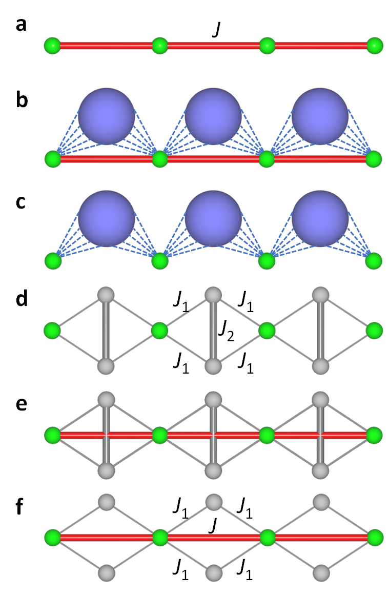
Figure 1: Schematic diagrams of decorated Ising chains. (a) The original ordinary Ising chain Ising1925 , which consists of the Ising spins (green balls) with the ferromagnetic interaction $J>0$ (red bonds). (b) The decoration consists of arbitrary finite-size sublattices (big blue balls) which are coupled to the ordinary chain by the Ising-type interactions (dotted lines). (c) Decorated Ising chain with the $J$ bonds neglected 005_Galisova_PRE_15_double-tetrahedral-chain ; 007_Torrico_PRA_16_Ising-XYZ-diamond-chain ; 009_review_Souza_SSC_18_Ising-XYZ-diamond-chain_double-tetrahedral-chain-spin-electron ; 010_Carvalho_JMMM_18_Ising-XYZ-diamond-chain_quantum-entanglement ; 011_Rojas_BJP_20_Ising-Heisenberg-tetrahedral_diamond ; 013_Rojas_PRE_19_previous_4_models ; 014_Rojas_JPC_20_Ising–Heisenberg_spin-1-double-tetrahedral-chain ; 015_Strecka_APPA_20_Ising-diamond-chain ; 015-7_Canova_CzechoslovakJP_04_Ising–Heisenberg_diamond_chain ; 015-8_Canova_JPC_06_Ising–Heisenberg-spin-S-diamond-chain ; 017_Krokhmalskii_PA_21_3-previous-chains_effective_model ; 016_Strecka_book_chapter . (d) The Ising diamond chain for $J=0$ 016_Strecka_book_chapter ; 015_Strecka_APPA_20_Ising-diamond-chain , in which the decorated Ising spins (grey balls) utilize the antiferromagnetic interactions $J_{1}<0$ and $J_{2}<0$ (grey bonds) to form triangles, yielding geometric frustration. (e) The Ising diamond chain with ferromagnetic $J>0$ studied here. (f) The Ising diamond chain without geometric frustration for $J_{2}=0$.

Author Information The author declares no competing interests. Correspondence and requests for materials should be addressed to W.Y. (wyin@bnl.gov).

References

- (1) Ising, E. Beitrag zur theorie des ferromagnetismus. Zeitschrift für Physik 31, 253–258 (1925). URL https://doi.org/10.1007/BF02980577.
- (2) Mattis, D. C. & Swendsen, R. Statistical Mechanics Made Simple (WORLD SCIENTIFIC, 2008), 2nd edn. URL https://www.worldscientific.com/doi/abs/10.1142/6670. eprint https://www.worldscientific.com/doi/pdf/10.1142/6670.
- (3) Mattis, D. C. The Theory of Magnetism II (Springer, Berlin, Heidelberg, 1985). URL https://doi.org/10.1007/978-3-642-82405-0.
- (4) Baxter, R. J. Exactly Solved Models in Statistical Mechanics (Academic Press, 1982).
- (5) Huang, K. Statistical mechanics (John Wiley & Sons, 2008).
- (6) Schneidman, E., Berry, M. J., Segev, R. & Bialek, W. Weak pairwise correlations imply strongly correlated network states in a neural population. Nature 440, 1007–1012 (2006). URL http://dx.doi.org/10.1038/nature04701.
- (7) Gálisová, L. & Strečka, J. Vigorous thermal excitations in a double-tetrahedral chain of localized ising spins and mobile electrons mimic a temperature-driven first-order phase transition. Phys. Rev. E 91, 022134 (2015). URL https://link.aps.org/doi/10.1103/PhysRevE.91.022134.
- (8) Torrico, J., Rojas, M., de Souza, S. & Rojas, O. Zero temperature non-plateau magnetization and magnetocaloric effect in an ising-xyz diamond chain structure. Physics Letters A 380, 3655–3660 (2016). URL https://www.sciencedirect.com/science/article/pii/S0375960116305308.
- (9) de Souza, S. & Rojas, O. Quasi-phases and pseudo-transitions in one-dimensional models with nearest neighbor interactions. Solid State Communications 269, 131–134 (2018). URL https://www.sciencedirect.com/science/article/pii/S0038109817303319.
- (10) Carvalho, I., Torrico, J., de Souza, S., Rojas, M. & Rojas, O. Quantum entanglement in the neighborhood of pseudo-transition for a spin-1/2 ising-xyz diamond chain. Journal of Magnetism and Magnetic Materials 465, 323–327 (2018). URL https://www.sciencedirect.com/science/article/pii/S0304885317335114.
- (11) Rojas, O. A conjecture on the relationship between critical residual entropy and finite temperature pseudo-transitions of one-dimensional models. Brazilian Journal of Physics 50, 675–686 (2020). URL https://doi.org/10.1007/s13538-020-00773-8.
- (12) Rojas, O., Strečka, J., Lyra, M. L. & de Souza, S. M. Universality and quasicritical exponents of one-dimensional models displaying a quasitransition at finite temperatures. Phys. Rev. E 99, 042117 (2019). URL https://link.aps.org/doi/10.1103/PhysRevE.99.042117.
- (13) Rojas, O., Strečka, J., Derzhko, O. & de Souza, S. M. Peculiarities in pseudo-transitions of a mixed spin-(1/2, 1) ising–heisenberg double-tetrahedral chain in an external magnetic field. Journal of Physics: Condensed Matter 32, 035804 (2019). URL https://dx.doi.org/10.1088/1361-648X/ab4acc.
- (14) Strečka, J. Peculiarities in pseudo-transitions of a mixed spin-(1/2, 1) ising–heisenberg double-tetrahedral chain in an external magnetic field. Acta Physica Polonica A 137, 610 (2020). URL https://doi.org/10.12693/APhysPolA.137.610.
- (15) Čanová, L., Strečka, J. & Jaščur, M. Exact results of the ising-heisenberg model on the diamond chain with spin-1/2. Czechoslovak Journal of Physics 54, 579–582 (2004). URL https://doi.org/10.1007/s10582-004-0148-6.
- (16) Čanová, L., Strečka, J. & Jaščur, M. Geometric frustration in the class of exactly solvable ising–heisenberg diamond chains. Journal of Physics: Condensed Matter 18, 4967 (2006). URL https://dx.doi.org/10.1088/0953-8984/18/20/020.
- (17) Krokhmalskii, T., Hutak, T., Rojas, O., de Souza, S. M. & Derzhko, O. Towards low-temperature peculiarities of thermodynamic quantities for decorated spin chains. Physica A: Statistical Mechanics and its Applications 573, 125986 (2021). URL https://www.sciencedirect.com/science/article/pii/S0378437121002582.
- (18) Strečka, J. Pseudo-critical behavior of spin-1/2 ising diamond and tetrahedral chains, 63–86 (Nova Science Publishers, New York, 2020). URL "https://arxiv.org/abs/2002.06942". Preprint on arXiv:2002.06942.
- (19) Balents, L. Spin liquids in frustrated magnets. Nature 464, 199–208 (2010). URL https://doi.org/10.1038/nature08917.
- (20) Miyashita, S. Phase transition in spin systems with various types of fluctuations. Proceedings of the Japan Academy. Series B, Physical and biological sciences 86, 643–666 (2010). URL https://www.ncbi.nlm.nih.gov/pmc/articles/PMC3066537/.
- (21) Yin, W. Frustration-driven unconventional phase transitions at finite temperature in a one-dimensional ladder ising model. arXiv:2006.08921 (2020). URL https://arxiv.org/abs/2006.08921.
- (22) Yin, W. Finding and classifying an infinite number of cases of the practically perfect phase transitions with highly tunable novel properties in the ising model in one dimension. arXiv:2006.15087 (2020). URL https://arxiv.org/abs/2006.15087.
- (23) Hutak, T., Krokhmalskii, T., Rojas, O., Martins de Souza, S. & Derzhko, O. Low-temperature thermodynamics of the two-leg ladder ising model with trimer rungs: A mystery explained. Physics Letters A 387, 127020 (2021). URL https://www.sciencedirect.com/science/article/pii/S0375960120308872.
- (24) Yin, W.-G., Roth, C. R. & Tsvelik, A. M. Spin frustration and a ‘half fire, half ice’ critical point from nonuniform g-factors. arXiv:1510.00030 (2015). URL https://doi.org/10.48550/arXiv.1510.00030.
- (25) Bell, G. M. Ising ferrimagnetic models. i. Journal of Physics C: Solid State Physics 7, 1174 (1974). URL https://dx.doi.org/10.1088/0022-3719/7/6/016.
- (26) Emery, V. J. & Kivelson, S. A. Importance of phase fluctuations in superconductors with small superfluid density. Nature 374, 434–437 (1995). URL https://doi.org/10.1038/374434a0.
- (27) Ortega-Zamorano, F., Montemurro, M. A., Cannas, S. A., Jerez, J. M. & Franco, L. Fpga hardware acceleration of monte carlo simulations for the ising model. IEEE Transactions on Parallel and Distributed Systems 27, 2618–2627 (2016). URL https://arxiv.org/abs/1602.03016.
- (28) Pierangeli, D., Marcucci, G. & Conti, C. Large-scale photonic ising machine by spatial light modulation. Phys. Rev. Lett. 122, 213902 (2019). URL https://link.aps.org/doi/10.1103/PhysRevLett.122.213902.
- (29) Lee, J., Carbone, M. R. & Yin, W. Machine learning the spectral function of a hole in a quantum antiferromagnet. Phys. Rev. B 107, 205132 (2023). URL https://link.aps.org/doi/10.1103/PhysRevB.107.205132.