Cosmology in Lorentzian Regge calculus: causality violations, massless scalar field and discrete dynamics

Abstract

We develop a model of spatially flat, homogeneous and isotropic cosmology in Lorentzian Regge calculus, employing 4-dimensional Lorentzian frusta as building blocks. By examining the causal structure of the discrete spacetimes obtained by gluing such 4-frusta in spatial and temporal direction, we find causality violations if the sub-cells connecting spatial slices are spacelike. A Wick rotation to the Euclidean theory can be defined globally by a complexification of the variables and an analytic continuation of the action. Introducing a discrete free massless scalar field, we study its equations of motion and show that it evolves monotonically. Furthermore, in a continuum limit, we obtain the equations of a homogeneous scalar field on a spatially flat Friedmann background. Vacuum solutions to the causally regular Regge equations are static and flat and show a restoration of time reparametrisation invariance. In the presence of a scalar field, the height of a frustum is a dynamical variable that has a solution if causality violations are absent and if an inequality relating geometric and matter boundary data is satisfied. Edge lengths of cubes evolve monotonically, yielding a contracting or an expanding branch of the universe. In a small deficit angle expansion, the system can be deparametrised via the scalar field and a continuum limit of the discrete theory can be defined which we show to yield the relational Friedmann equation. These properties are obstructed if higher orders of the deficit angle are taken into account. Our results suggest that the inclusion of timelike sub-cells is necessary for a causally regular classical evolution in this symmetry restricted setting. Ultimately, this works serves as a basis for forthcoming investigations on the cosmological path integral within the framework of effective spin foams.

1 Introduction

Deriving quantum cosmology from full quantum gravity is an important research goal for multiple reasons: the large degree of symmetry greatly reduces the complexity of the considered quantum gravity model. As a result, analytical studies and numerical simulations are more accessible. Moreover, this simplified setting permits tackling of conceptual questions, such as matter coupling, causal structure of (quantum) spacetime, recovery of semi-classical physics and, in approaches that feature discrete variables, remnants of continuum symmetries and the definition of a continuum limit. On the phenomenological side, quantum effects are expected to become relevant for physics of the early Universe, in particular close to the Big Bang. These effects might leave traces detectable in cosmological observations such as that of the CMB spectrum Planck:2018vyg , therefore offering a promising testing ground for quantum gravity theories.

Quantum gravity approaches with discrete degrees of freedom, such as spin foam models Perez:2013uz , loop quantum gravity (LQG) Ashtekar:2021kfp and group field theories (GFTs) Oriti:2006ts ; Freidel:2005qe , face two major challenges in this endeavour. First, the identification of macroscopic cosmological variables from the microscopic ones. This involves either a coarse-graining procedure as in GFT condensate cosmology Marchetti:2020umh ; Oriti:2016qtz ; Gielen:2016dss ; Jercher:2021bie or a symmetry reduction. The latter can be performed either before quantising, i.e. on the classical configuration space, as in loop quantum cosmology Agullo:2016tjh or after quantising, i.e. on the quantum configuration space, as e.g. in Bahr:2017bn ; Bianchi:2010ej . The second challenge is to define the dynamics of cosmological observables in the absence of a background manifold. Evolution of observables can only be described with respect to other dynamical degrees of freedom, leading to a relational formulation Rovelli:1990ph ; Rovelli:2001bz ; Dittrich:2005kc ; Hoehn:2019fsy .

In spin foams a cosmological subsector is identified by symmetry reducing to those quantum geometric variables which capture the desired spatially homogeneous and isotropic dynamics. In earlier works of spin foam cosmology Bianchi:2010ej ; Bianchi:2011ym ; Rennert:2013pfa ; Sarno:2018ses the cosmological dynamics were examined in particular transition amplitudes of so-called dipole states and petal states in the full EPRL spin foam model Engle:2007em ; Engle:2008fj . Recently, investigations were conducted to define a Hartle-Hawking no boundary wavefunction by computing the transition from nothing to an equilateral spatial triangulation in the EPRL model Gozzini:2019nbo ; Frisoni:2022urv ; Frisoni:2023lvb . Other examples of symmetry reduced spin foam models, not necessarily tailored to cosmology, are given by the cuboid Bahr:2015gxa ; Bahr:2016dl ; Bahr:2017klw , frusta Bahr:2017bn ; Bahr:2018ewi ; Bahr:2018gwf ; Jercher:2023rno and parallel-epiped models Assanioussi:2020fml . Due to the numerical challenges accompanying the evaluation of symmetry reduced quantum amplitudes for large spins Allen:2022unb , resorting to semi-classical amplitudes appeared fruitful in advancing explicit computations. Following this line of research, effective spin foams Asante:2021zzh ; Asante:2020iwm ; Asante:2020qpa have been applied to the cosmological setting in Dittrich:2023rcr ; Dittrich:2021gww ; Asante:2021phx extending earlier works of quantum Regge cosmology CorreiadaSilva:1999cg ; CorreiadaSilva:1999es ; Hartle:1985wr ; Hartle:1986up ; Liu:2015gpa . As the semi-classical geometry, one frequently considers an equilateral triangulation of the $3$-sphere which describe positively curved spatial slices and which evolves into a $3$-sphere of different size, describing the evolution of the scale factor.

Recent studies of effective spin foams (and associated classical Regge calculus) Asante:2021zzh ; Dittrich:2021gww ; Asante:2021phx ; Dittrich:2023rcr have revealed several intriguing physical features already present in these simplified cosmological models. The triangulated spacetimes are piece-wise Lorentzian, i.e. its building blocks are pieces of flat Minkowski spacetime glued together. This allows for a plethora of configurations and different cases, since sub-simplices can be either space- or timelike. In turn, this can lead to causally irregular configurations in the form of more or less than two light cones located at spacelike sub-simplices, some of which can be interpreted as topology change. In the cosmological setting mentioned above, one typically obtains causally regular configurations if the edges connecting the spatial $3$-spheres are timelike. Such a case is similar to triangulations encountered in Causal Dynamical Triangulations (CDT) Ambjorn:2012jv ; Loll:2019rdj . However, if all building blocks are spacelike causally irregular configurations generically appear. To find a causally regular subsector of the full quantum theory therefore suggests the investigation of causally extended spin foam models such as the Conrady-Hnybida (CH) extension of the Lorentzian EPRL model Conrady:2010kc ; Conrady:2010vx or the completion of the Barrett-Crane model Jercher:2022mky . Unfortunately these models are not as computationally mature as their purely spacelike formulation and open questions regarding their asymptotics remain (see Kaminski:2017eew ; Liu:2018gfc ; Simao:2021qno for the asymptotics of the EPRL-CH model).

In this article we are proposing a different spatial triangulation to describe cosmology. Instead of a constantly curved space, we propose flat space described by a cubulation with toroidal topology. These tori are connected in spacetime by so-called frusta, higher-dimensional trapezoids, which interpolate between cubes of different size. In fact, we are adapting the proposal from the Euclidean EPRL model Bahr:2017bn to Lorentzian Regge calculus, where the 3-frusta can be either space- or timelike. Similar to the triangulated $3$-spheres, we will show that causally irregular structures can occur if some building blocks become spacelike; in most such cases the associated Regge action is complex and classical solutions do not exist. In fact, in vacuum spacetimes, the only permitted solutions are static spacetimes, where the spatial slices are connected by timelike edges. These solutions are flat and thus exhibit a reparametrisation invariance Rocek:1981ama ; Rocek:1982tj : the time elapsed between two slices is arbitrary, which can be related to a change of lapse function. In such a setting, taking the continuum limit is trivial, both in temporal and spatial directions.

The second direction we are exploring here is coupling a massless scalar field to the classical Regge action, following the suggestion by Hamber Hamber:1993gn . Our goal is to investigate whether this scalar field can be used to deparametrise the theory, i.e. express the cosmological dynamics relationally in terms of the scalar field and thus in a diffeomorphism invariant manner. In our case this would imply that the dependence on the height variables, essentially the proper time elapsed between two spatial slices, drops out and is replaced by differences of the scalar field. If this is the case, the foliation we have chosen would be exactly the one singled out by the scalar field. This insight should however be taken with a grain of salt as we have made several simplifying assumptions. In this article, we will explicitly solve the classical dynamics of the scalar field and observe a strictly monotonic behaviour (depending on the boundary values of the scalar field and the discrete geometry).

The question whether the theory can be deparametrised is more subtle: as soon as the scalar field boundary data are not equal, we will show that the Regge geometry is no longer flat and thus loses the reparametrisation invariance. Hence, the height variables become dynamical degrees of freedom and are uniquely fixed by the equations of motion. While we may still attempt to express the dynamics in terms of the scalar field, an explicit dependence on the height variables remains. The situation is further complicated by the transcendental nature of the Regge equations. To better understand how the symmetry is broken (and eventually restored in a continuum limit), we expand the equations of motion in a Taylor series of small deficit angles. To lowest order in the deficit angles, the system is reparametrisation invariant and the dependence on the height variables can be replaced by expressing the dynamics with respect to scalar field differences. This breaks down at higher orders of the deficit angles, which is not surprising. Thus, we expect to restore the symmetry in a continuum limit, in which the deficit angles become small and eventually vanish. We study this continuum limit and recover the classical solution of spatially flat cosmology with non-vanishing massless scalar field.

Moreover, in most cases adding a scalar field leads to a regular causal structure. The solutions to the Regge equations are not flat, where the spatial slices are connected by timelike edges. Hence the Regge action is purely real and the geometry causally regular. The situation changes if we change the sign in front of the scalar field action. Then, no classical solutions can be found: in the causally regular sector, the Regge equations have no solutions. In the irregular sector, the Regge action is complex and the equations of motion for real and imaginary part are not simultaneously solved for real length variables.

In short, the purpose of this article is to define a spatially flat cosmological subsector in Lorentzian Regge calculus coupled to a massless scalar field. The thorough classical analysis of the system we are about to present is to prepare the eventual examination of the quantum system as a path integral in effective spin foams. Our article is organised as follows: in Sec. 2 we introduce the triangulation and Lorentzian Regge calculus, discuss irregular causal structures and define a Wick rotation. Sec. 3 introduces the minimally coupled scalar field in the discrete, its equations of motion, continuum limit and Wick rotation as well. In Sec. 4 we study the Regge equations of motion for multiple time steps in vacuum and with matter, we linearise around small deficit angles and discuss deparametrisation as well as causality violations and their relation to matter. We close in Sec. 5 with a discussion and conclusion.

2 Spatially flat cosmology in Regge calculus

Regge calculus Regge:1961ct is a discrete gravitational theory, introduced for simplicial manifolds $\Delta$ with dynamical variables being the length of edges $\{l_{e}\}$. In four dimensions, to which we restrict to in the remainder, a simplicial manifold consists of $4$-simplices $\sigma\in\Delta$ which are internally flat, i.e. they can be embedded into Minkowski space $\mathbb{R}^{1,3}$. Curvature is located at the triangles $t\in\Delta$ and captured by deficit angles $\delta_{t}(\{l_{e}\})$, which lie in a two-dimensional space orthogonal to $t$. In the Lorentzian setting, this space is two-dimensional Minkowski space $\mathbb{R}^{1,1}$ or two-dimensional Euclidean space $\mathbb{R}^{2}$, depending on the triangle $t$ being spacelike or timelike, respectively. To define Lorentzian angles we follow in this work the conventions of Sorkin:2019llw ; Asante:2021zzh which ensure additivity of angles as in Euclidean space. The deficit angles can then be expressed as

$$\delta_{t}^{\mathrm{E}}=2\pi-\sum_{\sigma\supset t}\psi_{\sigma,t}^{\mathrm{E}},\qquad\delta_{t}^{\mathrm{L},\pm}=\mp i2\pi-\sum_{\sigma\supset t}\psi_{\sigma,t}^{\mathrm{L},\pm},$$ (1)

where the $\psi_{\sigma,t}$ are dihedral angles, i.e. the angles between normal vectors $N_{\tau}$ of tetrahedra $\tau\supset t$ within the $4$-simplex $\sigma$. Here, the “$\pm$” indicates a choice of sign which becomes important if the imaginary parts of the Lorentzian dihedral angles do not sum up to $\pm i2\pi$. As we will discuss in more detail in Sec. 2.4, such configurations are interpreted as causally irregular, representing for instance spatial topology change Sorkin:2019llw ; Asante:2021zzh ; Asante:2021phx .

The bulk action of Lorentzian Regge calculus is given by Sorkin:2019llw

$$S_{\mathrm{R}}[\{l_{e}\}]=\sum_{t\in\Delta:\text{ tl}}\absolutevalue{A_{t}(\{l_{e}\})}\delta_{t}^{\mathrm{E}}(\{l_{e}\})+\sum_{t\in\Delta:\text{ sl}}\absolutevalue{A_{t}(\{l_{e}\})}\delta_{t}^{\mathrm{L},\pm}(\{l_{e}\}),$$ (2)

where $\absolutevalue{A_{t}}$ is the absolute value of the area associated to the triangle $t$. In the presence of a boundary $\partial\Delta$, the Regge action attains boundary terms such that overall additivity is ensured. The equations of motion are given by

$$\partialderivative{S_{\mathrm{R}}}{l_{e}}=\sum_{t}\partialderivative{\absolutevalue{A_{t}}}{l_{e}}\delta_{t}=0,$$ (3)

where the Schläfli identity has been imposed, i.e. $\sum_{t}\absolutevalue{A_{t}}\partialderivative{\delta_{t}}{l_{e}}=0$.

There exist several related formulations of Regge calculus in terms of different variables Barrett:1994ba ; Dittrich:2008hg , most notably area Regge calculus Asante:2018wqy ; Makela:2000ej ; Barrett:1997tx , where the dihedral angles are a function of areas rather than lengths. Since $10$ lengths uniquely characterise a $4$-simplex while $10$ areas do not and since a triangulation contains in general more triangles than edges, area variables do in general lead to different equations of motion than length variables. As shown in Barrett:1997tx ; Dittrich:2008va ; Asante:2021zzh , area variables need to be further constrained to yield the dynamical equations of length Regge calculus. This idea lies at the heart of effective spin foams Asante:2021phx ; Asante:2020iwm ; Asante:2020qpa , where a gravitational path integral is implemented for area Regge calculus, where the area-length constraints are imposed ad-hoc via Gaussians. For simple, symmetry reduced systems, such as the cosmological models in Asante:2021phx ; Dittrich:2023rcr ; Dittrich:2021gww as well as the model we construct in the following, the relation of area and length is globally invertible and the constraints mentioned above trivialise.

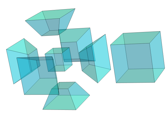
Figure 1: The boundary of a $4$-frustum, consisting of two $3$-cubes and six equal boundary $3$-frusta, connecting the cubes. Not explicitly visualised here, the two $3$-cubes lie in different spacelike hypersurfaces and have a timelike separation.

Goal of this section is to set up a Regge action for spatially flat and isotropic cosmology. To that end, we consider at the level of combinatorics a special class of simplicial manifolds which consist of triangulated $4$-dimensional cuboids. We assume that each $4$-dimensional triangulated polytope admits an analogue of foliation into spacelike hypersurfaces, that is, there are two $3$-dimensional triangulated polytopes at different instances of time, connected by six $3$-dimensional triangulated polytopes. Spatial homogeneity translates to the requirement that every $3$-polytope in a fixed spacelike slice is the same. Isotropy is imposed by requiring the six faces of spacelike $3$-polytopes to be equal. Finally, imposing spatial flatness fixes the $4$-dimensional building block to be a triangulated Lorentzian $4$-frustum, being the $4$-dimensional generalisation of a trapezoid. A Lorentzian $4$-frustum consists of two spacelike $3$-cubes in different spacelike hypersurfaces connected by six boundary $3$-frusta, see Fig. 1 for a visualisation. The requirements of spatial flatness, homogeneity and isotropy are so restrictive that the entire geometry of a triangulated $4$-frustum can be captured by the length of the $3$-cubes, $s_{0}$ and $s_{1}$, and its height $H$, defined as the distance between the midpoints of the two $3$-cubes (see Fig. 2 for a $3$-dimensional depiction).

Deficit angles at subdividing triangles vanish as the inside of the $4$-frustum and its contained sub-cells is constrained to be flat. Hence, the Regge action associated to this type of restricted triangulated geometries effectively reduces to a generalised Regge action of $4$-frusta geometries, the $2$-dimensional building blocks of which are squares and trapezoids. Henceforth, we focus on $4$-frusta geometries and neglect any further flat triangulation.

Gluing $4$-frusta along boundary $3$-frusta in spatial direction and along boundary $3$-cubes in temporal direction, one obtains an extended discrete cosmological spacetime with cubulated slices labelled by $n\in\{0,...,M\}$. We say that a $4$-frustum lies in a “slab” between slices $n$ and $n+1$.

In the following three sections, we characterise the geometry of Lorentzian $4$-frusta more explicitly to ultimately set up the action for spatially flat cosmology in Lorentzian Regge calculus in Sec. 2.3.

2.1 Lorentzian frustum

In a Lorentzian setting, the edges, trapezoids and $3$-frusta connecting slices $n$ and $n+1$ can be either of spacelike or timelike character, reflected in the sign of the squared length, area and $3$-volume, respectively. In the following, we express these geometric quantities as functions of $(s_{n},s_{n+1},H_{n})$ and show under which conditions the building blocks are spacelike or timelike.

Figure 2: Depiction of a $4$-frustum with one spatial dimension suppressed. Spacelike edges of $3$-cubes, lying in different spacelike hypersurfaces, have a length of $s_{n}$ and $s_{n+1}$, respectively. The height $H_{n}$ of a $4$-frustum is defined as the distance between the midpoints of the $3$-cubes.

Edges.

Edges contained in trapezoids which thus connect cubes that lie in distinct slices $n$ and $n+1$ have a squared edge length given by

$$l_{n}^{2}=3\left(\frac{s_{n}-s_{n+1}}{2}\right)^{2}-H_{n}^{2},$$ (4)

and therefore we have that:

edge is timelike if	$l_{n}^{2}<0$	$\Leftrightarrow$	$H_{n}^{2}>\frac{3}{4}(s_{n}-s_{n+1})^{2}$,
edge is spacelike if	$l_{n}^{2}>0$	$\Leftrightarrow$	$H_{n}^{2}<\frac{3}{4}(s_{n}-s_{n+1})^{2}$.

Trapezoids.

The squared area $k_{n}^{2}$ of a trapezoid is given by

$$k_{n}^{2}=\left(\frac{s_{n}+s_{n+1}}{2}\right)^{2}\left[\left(\frac{s_{n}-s_{n+1}}{\sqrt{2}}\right)^{2}-H_{n}^{2}\right],$$ (5)

from which we extract that:

trapezoid is timelike if	$k_{n}^{2}<0$	$\Leftrightarrow$	$H_{n}^{2}>\frac{1}{2}(s_{n}-s_{n+1})^{2}$,
trapezoid is spacelike if	$k_{n}^{2}>0$	$\Leftrightarrow$	$H_{n}^{2}<\frac{1}{2}(s_{n}-s_{n+1})^{2}$.

$\mathbf{3}$-frusta.

To determine the signature and the $3$-volume of $3$-frusta, we consider first the squared height of the $3$-frustum,

$$h_{n}^{2}=\left(\frac{s_{n}-s_{n+1}}{2}\right)^{2}-H_{n}^{2}.$$ (6)

Then, the signature of the $3$-frustum is determined by the signature of its height:

$3$-frustum is timelike if	$h_{n}^{2}<0$	$\Leftrightarrow$	$H_{n}^{2}>\frac{1}{4}(s_{n}-s_{n+1})^{2}$,
$3$-frustum is spacelike if	$h_{n}^{2}>0$	$\Leftrightarrow$	$H_{n}^{2}<\frac{1}{4}(s_{n}-s_{n+1})^{2}$.

Using the squared height of the $3$-frustum, $h_{n}^{2}$, one can express the squared $3$-volume as

$$v_{n}^{2}=\frac{(s_{n}^{2}+s_{n}s_{n+1}+s_{n+1}^{2})^{2}}{9}h_{n}^{2}=\frac{(s_{n}^{2}+s_{n}s_{n+1}+s_{n+1}^{2})^{2}}{9}\left[\left(\frac{s_{n}-s_{n+1}}{2}\right)^{2}-H_{n}^{2}\right].$$ (7)

$\mathbf{4}$-frusta.

Lastly, the squared $4$-volume of a $4$-frustum is given by

$$V_{n}^{2}=\left(\frac{s_{n}+s_{n+1}}{2}\right)^{4}(s_{n}-s_{n+1})^{2}H_{n}^{2}.$$ (8)

As a building block of top dimension, the Lorentzian $4$-frustum is constrained to have a positive $4$-volume, yielding the condition of a positive squared $4$-height, i.e. $H_{n}^{2}>0$. If $H_{n}^{2}<0$, the $4$-frustum can only be embedded in $4$-dimensional Euclidean space.

Summarizing, the causal character of the lower-dimensional sub-cells is determined by the difference of spacelike edge length $s_{n}$ and $s_{n+1}$ relative to the $4$-dimensional height $H_{n}$. Depicted in Fig. 3, these relations are consistent with the fact that spacelike cells can only contain spacelike sub-cells while timelike sub-cells need always to be contained in timelike cells. The region of $H_{n}^{2}>0$ corresponds to the Lorentzian sector of the theory while $H_{n}^{2}<0$ is associated to the Euclidean sector. As we argue in Sec. 2.5, $H_{n}$ is naturally associated to the lapse function $N$ which, in the simple context of homogeneous cosmology, relates the Lorentzian and Euclidean sector via an analytical continuation, commonly referred to as Wick rotation.

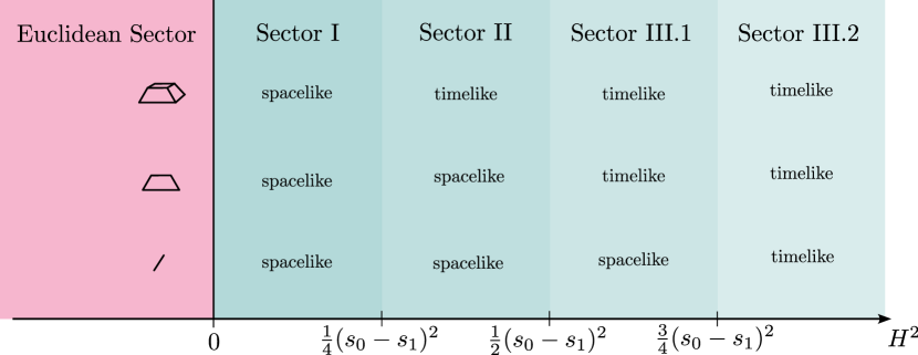
Figure 3: Sectors, determined by the relation of height $H$ and difference in spacelike edge length $(s_{0}-s_{1})$, in which the sub-cells of Lorentzian $4$-frusta take different signature.

2.2 Lorentzian angles

Following the introduction of Regge calculus at the beginning of this section, dihedral and deficit angles form a crucial ingredient for setting up the Lorentzian Regge action. In the restricted setting we consider here, there are two types of dihedral angles, associated either to spacelike squares or to trapezoids connecting slices. Crucially, the explicit expressions of these angles depends on the causal characters of sub-cells of the $4$-frustum and thus on the relative size of the variables $(s_{n},s_{n+1},H_{n})$. In the following, we provide a list of the dihedral angles for the various cases, using the definitions of Lorentzian angles as given in Asante:2021zzh . For a more detailed derivation, see Appendix A.

Dihedral angles at squares.

Cubes lie in spacelike hypersurfaces such that the squares contained in it must also be spacelike. As a consequence, the space orthogonal to a square is two-dimensional Minkowski space $\mathbb{R}^{1,1}$. In that space, the dihedral angle between the $3$-cube and the $3$-frustum meeting at that square is given by the Lorentzian angle between the respective projected normal vectors. While the normal vector to a $3$-cube is always timelike the signature of the vector normal to the $3$-frustum can be either spacelike or timelike, opposite to the signature of the $3$-frustum. Within a $4$-frustum, we refer to the dihedral angle located at the (past) $n$-th, respectively the (future) $(n+1)$-th slice as $\varphi_{nn+1}$ and $\varphi_{n+1n}$. Their explicit definitions in terms of the variables $(s_{n},s_{n+1},H_{n})$ are given by

$$\varphi_{nn+1}=\begin{cases}-\cosh^{-1}\left(\frac{s_{n+1}-s_{n}}{\sqrt{(s_{n}-s_{n+1})^{2}-4H_{n}^{2}}}\right)&\mathrm{if}\quad H_{n}^{2}<\frac{1}{4}(s_{n}-s_{n+1})^{2}\quad\mathrm{and}\quad s_{n}<s_{n+1},\\[10.0pt] \cosh^{-1}\left(\frac{s_{n}-s_{n+1}}{\sqrt{(s_{n}-s_{n+1})^{2}-4H_{n}^{2}}}\right)\mp i\pi&\mathrm{if}\quad H_{n}^{2}<\frac{1}{4}(s_{n}-s_{n+1})^{2}\quad\mathrm{and}\quad s_{n}>s_{n+1},\\[10.0pt] \sinh^{-1}\left(\frac{s_{n}-s_{n+1}}{\sqrt{4H_{n}^{2}-(s_{n}-s_{n+1})^{2}}}\right)\mp i\frac{\pi}{2}&\mathrm{if}\quad H_{n}^{2}>\frac{1}{4}(s_{n}-s_{n+1})^{2},\end{cases}$$ (9)

and

$$\varphi_{n+1n}=\begin{cases}-\cosh^{-1}\left(\frac{s_{n}-s_{n+1}}{\sqrt{(s_{n}-s_{n+1})^{2}-4H_{n}^{2}}}\right)&\mathrm{if}\quad H_{n}^{2}<\frac{1}{4}(s_{n}-s_{n+1})^{2}\quad\mathrm{and}\quad s_{n}>s_{n+1},\\[10.0pt] \cosh^{-1}\left(\frac{s_{n+1}-s_{n}}{\sqrt{(s_{n}-s_{n+1})^{2}-4H_{n}^{2}}}\right)\mp i\pi&\mathrm{if}\quad H_{n}^{2}<\frac{1}{4}(s_{n}-s_{n+1})^{2}\quad\mathrm{and}\quad s_{n}<s_{n+1},\\[10.0pt] \sinh^{-1}\left(\frac{s_{n+1}-s_{n}}{\sqrt{4H_{n}^{2}-(s_{n}-s_{n+1})^{2}}}\right)\mp i\frac{\pi}{2}&\mathrm{if}\quad H_{n}^{2}>\frac{1}{4}(s_{n}-s_{n+1})^{2}.\end{cases}$$ (10)

We observe that the real parts of the angles $\varphi_{nn+1}$ and $\varphi_{n+1n}$ are related by a minus sign. Furthermore, we notice that for a timelike frustum, the dihedral angles $\varphi$ do not depend on the sign of $s_{n}-s_{n+1}$. That is because the associated normal vector is spacelike and therefore insensitive to the time orientation.

Dihedral angles at trapezoids.

The dihedral between two $3$-frusta is located at a trapezoid, which can be either spacelike or timelike.

To a spacelike trapezoid, implying the inequality $H_{n}^{2}<\frac{1}{2}(s_{n}-s_{n+1})^{2}$, we associate the Lorentzian dihedral angle

$$\theta_{n}^{\mathrm{L}}=\begin{cases}-\cosh^{-1}\left(\frac{(s_{n}-s_{n+1})^{2}}{(s_{n}-s_{n+1})^{2}-4H_{n}^{2}}\right)&\mathrm{if}\quad H_{n}^{2}<\frac{1}{4}(s_{n}-s_{n+1})^{2},\\[10.0pt] -\cosh^{-1}\left(\frac{(s_{n}-s_{n+1})^{2}}{4H_{n}^{2}-(s_{n}-s_{n+1})^{2}}\right)\mp i\pi&\mathrm{if}\quad H_{n}^{2}>\frac{1}{4}(s_{n}-s_{n+1})^{2}.\end{cases}$$ (11)

To a timelike trapezoid, i.e. $H_{n}^{2}>\frac{1}{2}(s_{n}-s_{n+1})^{2}$, we associate the Euclidean angle

$$\theta_{n}^{\mathrm{E}}=\cos^{-1}\left(\frac{(s_{n}-s_{n+1})^{2}}{4H_{n}^{2}-(s_{n}-s_{n+1})^{2}}\right).$$ (12)

This completes the introduction of geometrical quantities of a single $4$-frustum lying in a slab bounded by spatial slices $n$ and $n+1$.

2.3 Lorentzian Regge action for spatially flat cosmology

To construct the Lorentzian Regge action for spatially flat homogeneous cosmology with $M$ spatial slices, we consider first the pure boundary Regge action $S_{\mathrm{R}}^{(n)}$ of a single $4$-frustum bounded by the slices $n$ and $n+1$. This is guided by the condition that the resulting action is additive for larger complexes, i.e. if $4$-frusta are glued together both in timelike and spacelike direction. The underlying $2$-complex defining the combinatorics of the model is hypercubic such that every square or trapezoid is shared by four $4$-frusta. As a result, the exterior boundary deficit angle for a single frustum is defined as

$$\delta^{\mathrm{E}} =\frac{\pi}{2}-\psi^{\mathrm{E}},$$ (13)

$$\delta^{\mathrm{L},\pm} =\mp i\frac{\pi}{2}-\psi^{\mathrm{L},\pm},$$ (14)

for angles in Euclidean space, $\psi^{\mathrm{E}}$, and Lorentzian space, $\psi^{\mathrm{L},\pm}$, respectively. Since the single $4$-frustum consists of six squares in slice $n$, twelve trapezoids and six squares in slice $n+1$, spatial homogeneity then implies that the Regge action is given by

$$S_{\mathrm{R}}^{(n)}[s_{n},s_{n+1},H_{n}] =6s_{n}^{2}\left(\mp i\frac{\pi}{2}-\varphi_{nn+1}\right)+6s_{n+1}^{2}\left(\mp i\frac{\pi}{2}-\varphi_{n+1n}\right)$$ (15)

$$+12\absolutevalue{k_{n}}\left[\Theta_{\mathrm{sl}}\left(\mp i\frac{\pi}{2}-\theta_{n}^{\mathrm{L}}\right)+\Theta_{\mathrm{tl}}\left(\frac{\pi}{2}-\theta_{n}^{\mathrm{E}}\right)\right],$$

where the $\Theta_{\mathrm{sl,tl}}$ are Heaviside functions that impose the trapezoid to be spacelike or timelike, respectively. An exemplary plot of the Regge action for $M=1$ is given in Fig. 4.

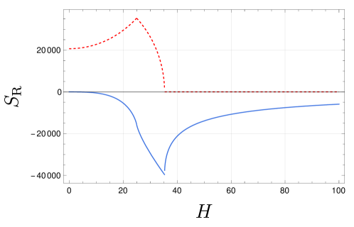
Figure 4: The real (solid blue) and imaginary (dashed red) parts of the Lorentzian Regge action of a single slice for boundary data $s_{1}=50$, $s_{2}=100$ plotted against the height $H$. The kinks in the Regge action stem from the Heaviside $\Theta$-functions that characterise the different causal sectors. Notice, that at the kinks, the Regge action is not differentiable and these points therefore do not correspond to non-trivial solutions of the equations of motion with respect to the variable $H$.

By construction, the $4$-frustum action of Eq. (15) is additive such that on a hypercubic complex with $L$ vertices in spatial direction and $M+1$ spatial slices, the action is given by

$$S_{\mathrm{R}}=L\sum_{n=0}^{M-1}S_{\mathrm{R}}^{(n)}[s_{n},s_{n+1},H_{n}].$$ (16)

Additivity of the action per slab implies that the equations of motion for a given geometric quantity, being either $s_{n}$ or $H_{n}$, will only depend on neighbouring geometric labels. We discuss the consequences of this slicing structure for the dynamics of the model in more detail in Sec. 4.

2.4 Causal (ir)regularity

Discussed at length in Asante:2021zzh ; Asante:2021phx , the Regge action can attain complex values when the imaginary parts of the dihedral angles at a face do not sum up to $\mp i2\pi$. This indicates the presence of causal irregularities in the form of a degenerate light cone structure. Two common examples for such configurations are the trouser singularity, where there are four instead of two light cones at the crotch of the trouser, or the yarmulke singularity, where there is no light cone at the tip. Choosing “$+$” in the convention of Lorentzian angles, the amplitude $\mathrm{e}^{iS_{\mathrm{R}}}$ is exponentially suppressed for trouser configurations and exponentially enhanced for yarmulke configurations and vice versa for the choice “$-$” Asante:2021zzh .

These two examples of causality violations are characterised by Lorentzian dihedral angles, located at the hinges of the cellular complex, and therefore referred to as hinge causality violations. It is furthermore proposed in Asante:2021phx , that the concept of hinge causality can be generalised to higher dimensions, referred to as edge and vertex causality. In the following, we study the three types of causality conditions for the present model and for the different signatures the sub-cells can take.

Hinge causality.

As indicated for the examples of trouser and yarmulke configurations, hinge causality violations are characterised by a non-vanishing imaginary part of the Lorentzian deficit angle. Each summand of $\mp i\frac{\pi}{2}$ for a dihedral angle counts one light cone crossing. Thus, there are exactly four light rays at a hinge if the imaginary parts of the dihedral angles sum up to $\mp i2\pi$. In the present setting, there are two different types of hinges to consider, squares and trapezoids, both of which are shared by four $4$-frusta. We consider these two types separately in the following.

At a square in slice $n$ there are four dihedral angles located, being two times the angle $\varphi_{nn-1}$ and two times the angle $\varphi_{nn+1}$. Following from Eqs. (9) and (10), the explicit form of these dihedral angles depends on the signature of the associated $3$-frusta. Modulo time inversion, there exist five distinct possibilities for the signature and orientation of the two $3$-frusta attached to the $n$-th slice. In Tab. 1, we summarise all the possibilities where “tl” indicates a timelike frustum and “sl $\uparrow(\downarrow)$” denotes a spacelike $3$-frustum with future (past) pointing $4$-dimensional normal vector.

$3$-frustum in slab $(n-1,n)$	tl	sl $\uparrow$	sl $\downarrow$	sl $\uparrow$	sl $\uparrow$
$3$-frustum in slab $(n,n+1)$	tl	tl	tl	sl $\uparrow$	sl $\downarrow$
regular causality	$\checkmark$	X	X	$\checkmark$	X

Table 1: Causal regularity $(\checkmark)$ or irregularity (X) for the dihedral angle located at a square in the $n$-th slice where “tl” and “sl” indicate a timelike, respectively spacelike $3$-frustum and where $\uparrow$ and $\downarrow$ indicate the relative time orientation of the $4$-dimensional normal vector. Since the choice of time orientation is arbitrary, the regularity of time reversed configurations is the same.

We find that the two causally regular configurations are given when either the $3$-frusta of the two slices are timelike or if they are spacelike with the same orientation. That is, causally irregular configurations are only obtained when $H_{n}^{2}<\frac{1}{4}(s_{n}-s_{n+1})^{2}$. Within a single given slice, where the dihedral angles $\varphi_{nn+1}$ are located at the boundary, the case of spacelike $3$-frusta yields imaginary contributions to the Regge action as there are either zero or four light cone crossings, depending on the orientation of the timelike normal vector. Only if another slice with spacelike $3$-frusta of the same orientation is glued, the imaginary parts can be compensated, yielding a real bulk deficit angle.

At a trapezoid in the slab between slice $n$ and $n+1$, there are four dihedral angles which are the same as the they lie in the same slab. If the trapezoid is timelike, the dihedral angles are Euclidean and we find for the bulk deficit angle

$$\delta^{\mathrm{E}}=2\pi-4\theta_{n}^{\mathrm{E}},$$ (17)

which is real by definition. If the trapezoid is spacelike, the dihedral angles are timelike and we have

$$\begin{cases}\mp i2\pi+4\cosh^{-1}\left(\frac{(s_{n}-s_{n+1})^{2}}{(s_{n}-s_{n+1})^{2}-4H_{n}^{2}}\right)&\mathrm{if}\quad H_{n}^{2}<\frac{1}{4}(s_{n}-s_{n+1})^{2},\\[10.0pt] \pm i2\pi+4\cosh^{-1}\left(\frac{(s_{n}-s_{n+1})^{2}}{4H_{n}^{2}-(s_{n}-s_{n+1})^{2}}\right)&\mathrm{if}\quad H_{n}^{2}>\frac{1}{4}(s_{n}-s_{n+1})^{2},\end{cases}$$ (18)

where we used Eqs. (12) and (11) for the definition of the dihedral angles $\theta_{n}^{\mathrm{E}}$ and $\theta_{n}^{\mathrm{L}}$, respectively. As a result, a spacelike trapezoid necessarily induces causality violations. The sign of the imaginary part of the deficit angle depends on the signature of the associated $3$-frustum and the choice of convention. As noted above, this sign determines whether the Lorentzian amplitudes $\mathrm{e}^{iS_{\mathrm{R}}}$ enhance or suppress trouser or yarmulke configurations, respectively.

Together with the results of Table 1, we observe that the configurations satisfying hinge causality are given by those which contain timelike trapezoids which already implies timelike $3$-frusta, that is $H_{n}^{2}>\frac{1}{2}(s_{n}-s_{n+1})^{2}$. Explicitly, the regular action is given by

$$S_{\mathrm{R}}^{(n)} =6(s_{n}^{2}-s_{n+1}^{2})\sinh^{-1}\left(\frac{s_{n+1}-s_{n}}{\sqrt{4H_{n}^{2}-(s_{n}-s_{n+1})^{2}}}\right)$$ (19)

$$+12\absolutevalue{k_{n}}\left[\frac{\pi}{2}-\cos^{-1}\left(\frac{(s_{n}-s_{n+1})^{2}}{4H_{n}^{2}-(s_{n}-s_{n+1})^{2}}\right)\right].$$

In the light of Fig. 3, Sector II exhibits hinge causality violations at trapezoids while Sector I shows such violations at trapezoids and squares. Finally, notice that hinge causality is not sensitive to the signature of the edges connecting the $n$-th and the $(n+1)$-th slice, and therefore, both Sector III.1 and III.2 are considered causally regular at the hinges.

Edge causality.

To set up the definition of edge causality, consider the plane $P$ orthogonal to a spacelike edge $e$ located at the midpoint of the edge. Moreover, let $\Sigma=\cup_{\sigma\supset e}\sigma$ be the union of $4$-polytopes sharing $e$. The intersection $P\cup\Sigma$ results in a discrete $3$-dimensional Lorentzian space with spherical boundary, whose single bulk vertex is the midpoint of the edge $e$. Following the definition of Asante:2021phx , the causal structure at the edge is said to be regular, if there are exactly two, one past and one future pointing, light cones emanating from the midpoint of $e$.

In the present setting there are two types of spacelike edges. One is given by edges that lie on the boundary of $3$-cubes. The other is given by edges connecting neighbouring slices, which are only spacelike if the inequality $H_{n}^{2}<\frac{3}{4}(s_{n}-s_{n+1})^{2}$ holds, as Tab. 3 shows. Due to the hypercubical combinatorics, an edge is shared by eight $4$-frusta. We discuss the two types of edge causality in the following.

Forming the intersection of the plane orthogonal to a spacelike edge $e$ inside a cube with a single $4$-frustum yields a $3$-frustum. Because of projecting out one dimension, the resulting $3$-frustum has a height $H_{n}$ and the squared length of its edges connecting two neighbouring slices is given by the squared height ${}_{(2)}h_{n}^{2}$ of the original (before projection) trapezoids,

$${}_{(2)}h^{2}_{n}=\frac{(s_{n}-s_{n+1})^{2}}{2}-H_{n}^{2}.$$ (20)

Then, the $3$-dimensional space obtained from the intersection of the plane with all the $4$-frusta is given by eight $3$-frusta glued together with the midpoint of edge $e$ as vertex in the middle. From this picture, we conclude that there are exactly two light cones if very single upper $3$-frustum contains a portion of the upper light cone, and every single lower $3$-frustum contains a portion of the lower light cone, each of which is emanating from the vertex $e$. This is the case if the edges connecting slices are timelike, i.e. if ${}_{(2)}h_{m}^{2}<0$ with $m\in\{n-1,n\}$. Then, by gluing the $3$-frusta along their faces, the pieces of light cones add up to two regular light cones. If one of the edges is instead spacelike, for instance if ${}_{(2)}h_{n}^{2}<0$, then each of the four $3$-frusta between slice $n$ and $n+1$ sharing the edge $e$ contains an entire or no light cone at all. In total, there are therefore either zero or four entire light cones in between the slice $n$ and $n+1$ in the projected $3$-frustum, necessarily inducing a degenerate light cone structure. Therefore, the causal structure at spacelike edges lying in $3$-cubes is regular if and only if the trapezoid is timelike, i.e. if $H_{n}^{2}>\frac{1}{2}(s_{n}-s_{n+1})^{2}$. See Fig. 5 for an analogous $2$-dimensional depiction.

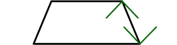
Figure 5: Light cones (green) emanating from vertices of a trapezoid with timelike (left) or spacelike (right) side edges. For a timelike edge, there is always one light ray inside the trapezoid at the upper and lower vertex. If the edge is spacelike, then the light cone of one vertex is fully contained inside the trapezoid while the light cone of the other vertex is fully outside the trapezoid. Causality violating configurations at spacelike squares, their edges or their vertices can be projected to two dimensions, yielding the figure on right-hand-side.

For a spacelike edge connecting slices $n$ and $n+1$, visualizing the orthogonal space and its intersection with the union of $4$-frusta is more involved. To study edge causality in this case, we explicitly compute the intersection of the plane with a single $4$-frustum. The total $3$-dimensional projected space is then obtained by gluing the eight intersections accordingly. A single $4$-frustum in $\mathbb{R}^{1,3}$ is defined by the sixteen vertices $\left(0,\pm\frac{s_{n}}{2},\pm\frac{s_{n}}{2},\pm\frac{s_{n}}{2}\right)$ and $\left(H_{n},\pm\frac{s_{n+1}}{2},\pm\frac{s_{n+1}}{2},\pm\frac{s_{n+1}}{2}\right)$. Choosing two vertices of different slices connected by an edge, e.g. $\left(0,\frac{s_{n}}{2},\frac{s_{n}}{2},\frac{s_{n}}{2}\right)$ and $\left(H_{n},\frac{s_{n+1}}{2},\frac{s_{n+1}}{2},\frac{s_{n+1}}{2}\right)$, its midpoint is given by

$$p=\left(0,\frac{s_{n}}{2},\frac{s_{n}}{2},\frac{s_{n}}{2}\right)+\frac{1}{2}\left(H_{n},\frac{s_{n+1}-s_{n}}{2},\frac{s_{n+1}-s_{n}}{2},\frac{s_{n+1}-s_{n}}{2}\right).$$ (21)

The plane $P$ orthogonal to the edge is defined as

$$P:-H_{n}x_{0}+\frac{s_{n+1}-s_{n}}{2}\sum_{i=1}^{3}x_{i}+d=0,$$ (22)

where $d(s_{n},s_{n+1},H_{n})$ is defined by demanding that $P$ contains the point $p$. Given the inequality $H_{n}^{2}<\frac{3}{4}(s_{n+1}-s_{n})^{2}$ and assuming that $s_{n}>s_{n+1}$, the intersection of the plane $P$ with every edge of the $4$-frustum is non-zero only at the points

$$q_{i}=-\frac{3(s_{n}-s_{n+1})^{2}-4H_{n}^{2}}{4(s_{n}-s_{n+1})}{\bf\it e}_{i}+\frac{s_{n}}{2}\sum_{j}{\bf\it e}_{j},$$ (23)

where ${\bf\it e}_{i}$ are $4$-dimensional unit vectors in the $i$-th spatial direction. Together with the point $p$, these four points form a tetrahedron with three timelike faces and one spacelike face which is spanned by the points $q_{i}$. Each such $3$-dimensional Lorentzian building block contains no light cone.

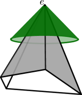
Figure 6: The space orthogonal to a spacelike edge $e$ connecting slices $n$ and $n+1$ with one dimension suppressed. Thus, in analogy, there are four flat timelike triangles instead of eight flat timelike tetrahedra depicted. The intersection of this piece-wise flat space with the light cone (in green) at the midpoint of edge $e$ is empty. Therefore, the causal structure at this edge is irregular.

The total $3$-dimensional space orthogonal to the spacelike edge is obtained by gluing all of the eight tetrahedra along their timelike faces, while the spacelike faces form the spherical boundary. A visualisation of this space with one spatial dimension suppressed is given in Fig. 6. As a result, this space does not contain a light cone at all and we conclude that edge causality is violated in every sector except Sector III.2.

Vertex causality.

At any vertex $v$ of the cellular complex, consider the union of all $4$-dimensional building blocks that contain that vertex. Then, the causal structure is said to be regular if the intersection of the light cone at $v$ with the boundary of the union are two disconnected spheres Asante:2021phx .

A vertex $v$ in a slice $n$ is shared by sixteen $4$-frusta, eight lying in the slab $(n-1,n)$ and eight lying in the slab $(n,n+1)$. If, for instance, the edge connecting slices $n$ and $n+1$ is spacelike, i.e. if $H_{n}^{2}<\frac{3}{4}(s_{n}-s_{n+1})^{2}$, then each $4$-frustum of the slab $(n,n+1)$ at $v$ contains either an entire or no light cone at all, depending on the sign of $s_{n}-s_{n+1}$. The analogous two-dimensional situation is depicted on the right-hand-side of Fig. 5. In this case, the vertex $v$ has either eight or zero upper light cones. The same applies to the case of a spacelike edge lying inside the slab $(n-1,n)$. Only if the edges are timelike, the light cone structure at the vertex $v$ is non-degenerate. Hence, vertex causality is violated in every sector except Sector III.2.

Summarizing, Sector I and II exhibit causality violating configurations at vertices, edges and hinges of the discrete Lorentzian spacetime. In Sector III.1 edge and vertex causality are violated which however remains unnoticed by the Regge action, which is only sensitive to hinge causality. Although the present setting is strongly simplified by symmetry, the results on causality violations suggest that higher-dimensional causality conditions imply lower-dimensional ones, e.g. vertex causality implies hinge causality. It is conceivable that this arises due to the dimensional reduction that results from the projections onto orthogonal subspaces of $k$-dimensional cells (e.g. edges, $k=1$ or hinges, $k=2$). However, we point out that the study of different causality violations and their interrelation in a more general setting remains an interesting question for future research.

2.5 Wick rotation

The symmetry reduced setting, and in particular the presence of the variable $H$ which is associated to the lapse function $N$, allows to define a Wick rotation between the Lorentzian theory, characterised by Eq. (15) and the Euclidean theory, defined by the action Bahr:2017bn

$$S_{\mathrm{R}}^{\mathrm{E}}= 6(s_{n}^{2}-s_{n+1}^{2})\left[\frac{\pi}{2}-\cos^{-1}\left(\frac{s_{n+1}-s_{n}}{\sqrt{4H_{n,\mathrm{E}}^{2}+(s_{n}-s_{n+1})^{2}}}\right)\right]$$ (24)

$$+ 12\absolutevalue{k_{n,\mathrm{E}}}\left[\frac{\pi}{2}-\cos^{-1}\left(\frac{(s_{n}-s_{n+1})^{2}}{4H_{n,\mathrm{E}}^{2}+(s_{n}-s_{n+1})^{2}}\right)\right].$$

In the context of Lorentzian Regge calculus, Ref. Asante:2021phx significantly advanced these studies by introducing a complexification of the Regge action that allows for a rigorous formulation of a Wick rotation.

Analogous to continuum studies Feldbrugge:2017kzv , the Wick rotation is performed by complexifying the lapse function, represented in the discrete setting by the squared height $H^{2}\rightarrow R^{2}\mathrm{e}^{i\alpha}$, where $\alpha$ is the rotation angle and $R^{2}$ is the modulus. Consequently, the area of trapezoids as well as the dihedral angles are complexified, denoted by $k_{n}(\alpha),\theta^{\pm}_{n}(\alpha)$ and $\varphi^{\pm}_{nn+1}(\alpha)$. The resulting Regge action can be analytically continued, which crucially depends on the structure of branch cuts. This in turn depends on the causal sector, i.e. on the difference of spacelike edge length $s_{n}-s_{n+1}$ relative to $R_{n}$.

In general, the complexified action for a single $4$-frustum, which we refer to as $\mathcal{S}_{\mathrm{R}}$, is of the form

$$\mathcal{S}_{\mathrm{R}}(\alpha)=6(s_{n}^{2}-s_{n+1}^{2})\left(\frac{\pi}{2}\pm\varphi_{nn+1}^{\pm}(\alpha)\right)+12k_{n}(\alpha)\left(\frac{\pi}{2}\pm\theta_{n}^{\pm}(\alpha)\right),$$ (25)

which can be analytically continued to Wick rotation angles $\alpha\in(-2\pi,2\pi]$ depending on its branch cuts. As elaborated in Asante:2021phx , to which we refer to for further details, causally regular configurations (i.e. $2R_{n}^{2}>(s_{n}-s_{n+1})^{2}$) show the following behaviour under Wick rotation

$$\mathcal{S}_{\mathrm{III}}(\alpha)\longrightarrow\begin{cases}\;-S_{\mathrm{R}}^{\mathrm{E}},&\quad\text{for $\alpha=0$}\,,\\ -iS_{\mathrm{R}}^{\mathrm{L}},&\quad\text{for $\alpha=-\pi$}\,,\\ \quad\,S_{\mathrm{R}}^{\mathrm{E}},&\quad\text{for $\alpha=2\pi$}\,,\\ \quad\!iS_{\mathrm{R}}^{\mathrm{L}},&\quad\text{for $\alpha=\pi$}\,,\end{cases}$$ (26)

where we remind the reader that the regular Lorentzian action does not depend on the choice of sign for Lorentzian angles.

For causality violating terms in Sector I, $4R_{n}^{2}<(s_{n}-s_{n+1})^{2}$, and II, $(s_{n}-s_{n+1})^{2}<4R_{n}^{2}<2(s_{n}-s_{n+1})^{2}$, the Wick rotation is sensitive to the direction from which the values $\alpha=\pm\pi$ are approached. In particular, it is shown in Asante:2021phx that

$$\mathcal{S}_{\mathrm{I,II}}(\alpha)\longrightarrow\begin{cases}-iS_{\mathrm{R}}^{\mathrm{L,+}},&\quad\text{for $\alpha\rightarrow-\pi\uparrow$}\,,\\ -iS_{\mathrm{R}}^{\mathrm{L,-}},&\quad\text{for $\alpha\rightarrow-\pi\downarrow$}\,,\\ \quad\!iS_{\mathrm{R}}^{\mathrm{L,+}},&\quad\text{for $\alpha\rightarrow\pi\uparrow$}\,,\\ \quad\!iS_{\mathrm{R}}^{\mathrm{L,-}},&\quad\text{for $\alpha\rightarrow\pi\downarrow$}\,,\end{cases}$$ (27)

where the Lorentzian actions $S_{\mathrm{R}}^{\mathrm{L},\pm}$ now explicitly depend on the choice of sign. Approaching the Euclidean sector at $\alpha=0,2\pi$, we notice that there exist two analytic extensions per sector, $\mathcal{S}_{\mathrm{I,II}}$ and $\mathcal{S}_{\mathrm{I,II}}^{\prime}$, agreeing with $\mathcal{S}_{\mathrm{III}}$ in the regions $\alpha\in(-\pi,\pi)$ and $\alpha\in(-2\pi,\pi)\cup(\pi,2\pi]$, respectively. Consequently,

$$\mathcal{S}_{\mathrm{I,II}}(0)=-S_{\mathrm{R}}^{\mathrm{E}},\qquad\mathcal{S}_{\mathrm{I,II}}^{\prime}(2\pi)=S_{\mathrm{R}}^{\mathrm{E}}.$$ (28)

In the other limiting cases, additional terms enter that depend on the number of light cone crossings. As explained above, Sector I shows causality violations at trapezoids and squares while Sector II is irregular only at trapezoids. As a result, the remaining limiting values of $\mathcal{S}_{\mathrm{I,II}}$ and $\mathcal{S}_{\mathrm{I,II}}^{\prime}$ are given by

$$\mathcal{S}_{\mathrm{I}}^{\prime}(0) =-S_{\mathrm{R}}^{\mathrm{E}}+2\pi\cdot 12\absolutevalue{k_{n}}-2\pi\cdot 6(s_{n}^{2}-s_{n+1}^{2})\,,$$ (29a)

$$\mathcal{S}_{\mathrm{II}}^{\prime}(0) =-S_{\mathrm{R}}^{\mathrm{E}}-4\pi\cdot 12\absolutevalue{k_{n}}\,,$$ (29b)

$$\mathcal{S}_{\mathrm{I}}(2\pi) =\;\;S_{\mathrm{R}}^{\mathrm{E}}-2\pi\cdot 12\absolutevalue{k_{n}}+2\pi\cdot 6(s_{n}^{2}-s_{n+1}^{2})\,,$$ (29c)

$$\mathcal{S}_{\mathrm{II}}(2\pi) =\;\;S_{\mathrm{R}}^{\mathrm{E}}+4\pi\cdot 12\absolutevalue{k_{n}}\,.$$ (29d)

In summary, the Lorentzian and Euclidean Regge actions are related via the Wick rotation procedure described in this section, where causality violating terms in the Lorentzian sector will also lead to changes in the Euclidean sector. This direct connection hinges on the existence of a foliation into spacelike hypersurfaces which, similar to the setting in CDT, allows for a global Wick rotation in a single parameter. It is nevertheless remarkable that the Lorentzian action obtained in Sec. 2.3 is the result of an ad hoc construction and still directly connected to the Euclidean action derived in Bahr:2017bn from the semi-classics of an underlying quantum geometric model. Although this result suggests that there may exist a symmetry restricted causally extended Lorentzian spin foam model whose semi-classical limit leads to the Lorentzian Regge action of spatially flat cosmology, the ultimate answer to this questions remains open. That is because the semi-classical limit of full Lorentzian spin foam models, being either the CH-extension of the EPRL model Conrady:2010vx ; Conrady:2010kc or the causal completion of the Barrett-Crane model Jercher:2022mky , is in general not well understood and subject to active research, see Simao:2021qno .

3 A minimally coupled massless scalar field

In this section, we introduce a minimally coupled massless scalar field to the cosmological model precedingly developed. Starting from a continuum perspective a scalar field, being a $0$-form, is discretised by placing it either on primary or dual vertices of the cellular complex Desbrun:2005ug . Since we assume spatial homogeneity also for the scalar field, it is for our purposes advantageous to discretise the scalar field on primal vertices, $\phi(t)\rightarrow\phi_{n}$, which therefore attains the index of the slice.

3.1 Discrete scalar field action

The continuum action for a free massless scalar field, minimally coupled to spatially flat cosmology, given in Eq. (80), is quadratic in fields and derivatives and exhibits translation and reflection symmetry. Following Hamber:2009wl ; Hamber:1993gn , we translate this action to the discrete setting. The scalar field action for a single $4$-frustum between slice $n$ and $n+1$ is then given by

$$S_{\phi}^{(n)}[\phi_{n},\phi_{n+1},s_{n},s_{n+1},H_{n}]=w_{n}(\phi_{n+1}-\phi_{n})^{2}.$$ (30)

Clearly, this action exhibits translation and reflection symmetry and is quadratic in the fields. Here, $w_{n}(s_{n},s_{n+1},H_{n})$ is a geometrical coefficient that plays the role of the continuum factor $\frac{a^{3}}{2N}$ in the discrete and scales like squared length. Therefore, we choose

$$w_{n}=\frac{1}{2H_{n}^{2}}\left(\frac{s_{n}+s_{n+1}}{2}\right)^{3}H_{n}=\frac{(s_{n}+s_{n+1})^{3}}{16H_{n}},$$ (31)

which yields the correct continuum limit of the coupled gravity and matter system, as we show in Sec. 4.3. The first expression of Eq. (31) is closest to the continuum, where $1/H_{n}^{2}$ encodes the discrete squared time derivative. The lengths $(s_{n}+s_{n+1})/2$ and the height $H_{n}$ characterise the volume of a $4$-dimensional cuboid which can be understood as the discretisation of the $4$-volume element $\sqrt{-g}$.

On an extended $2$-complex with $L$ spatial vertices and spatial $M+1$ slices, the total action for $\phi$ is given by

$$S_{\phi}=L\sum_{n=0}^{M-1}w_{n}(\phi_{n}-\phi_{n+1})^{2},$$ (32)

showing the same slicing structure as the Regge action in Eq. (16). This simplifies the equations of motion significantly, as the equation on the $n$-th slice does only depend on the dynamical quantities of the neighbouring slices $n-1$ and $n+1$.

3.2 Equations of motion

In this section, we consider the equations of motion of the scalar field on the homogeneous background with $M+1$ slices and fixed initial and final values $\phi_{0}$ and $\phi_{M}$. To that end, we perform the variation of $S_{\phi}$ in Eq. (32), yielding the system of equations

$$\phi_{n}(w_{n-1}+w_{n})-(\phi_{n-1}w_{n-1}+\phi_{n+1}w_{n})=0,\qquad n\in\{1,...,M-1\},$$ (33)

which can be solved for $\phi_{n}$, yielding

$$\phi_{n}=\frac{\phi_{n+1}\frac{1}{w_{n-1}}+\phi_{n-1}\frac{1}{w_{n}}}{\frac{1}{w_{n-1}}+\frac{1}{w_{n}}}.$$ (34)

Recursively, this system of equations can be solved for a single scalar field $\phi_{n}$ as a function of the boundary data $\phi_{0},\phi_{M}$ and the geometric quantities $\{s_{n},H_{n}\}$. For the first recursion step, we insert the equation for $\phi_{n-1}$ into the equation for $\phi_{n}$, yielding

$$\phi_{n}=\frac{\phi_{n+1}\left(\frac{1}{w_{n-2}}+\frac{1}{w_{n-1}}\right)+\phi_{n-2}\left(\frac{1}{w_{n}}\right)}{\sum\limits_{m=n-2}^{n}\frac{1}{w_{m}}}$$ (35)

Repeating these steps to “earlier” and “later” slices until one reaches the initial and final slices $0$ and $M$, respectively, the scalar field solutions is given by

$$\phi_{n}=\frac{\phi_{M}\mathcal{W}_{0}^{n-1}+\phi_{0}\mathcal{W}_{n}^{M-1}}{\mathcal{W}_{0}^{M-1}},$$ (36)

where we introduced the symbols

$$\mathcal{W}_{n_{1}}^{n_{2}}=\sum_{m=n_{1}}^{n_{2}}\frac{1}{w_{m}},$$ (37)

which explicitly depend on the geometric quantities $\{H_{n},s_{n}\}$. Clearly, scalar field solutions for boundary conditions $\phi_{0}=\phi_{M}$ are constant, i.e. $\phi_{n}=\phi_{0}$ for all $n\in\{0,...,M\}$.

To check for monotonicity, it is instructive to re-express the scalar field solutions in the following form

$$\phi_{n+1}-\phi_{n}=\frac{\frac{1}{w_{n}}}{\mathcal{W}_{0}^{M-1}}(\phi_{M}-\phi_{0}).$$ (38)

Since each $w_{m}$ is positive, following from Eq. (31), the scalar field evolves monotonically, the sign of which depends on the sign of $\phi_{M}-\phi_{0}$, i.e.

$$\mathrm{sgn}\left(\phi_{n+1}-\phi_{n}\right)=\mathrm{sgn}\left(\phi_{M}-\phi_{0}\right),\qquad\forall n\in\{0,...,N-1\}.$$ (39)

For the later purpose of deparametrising the system with respect to the scalar field, this is one of the crucial properties.

3.3 Continuum time limit

The simple form of the scalar field equations allows for a straightforward definition of a map from discrete to continuum variables. Since the scalar field equation is coupled non-trivially to the geometry via the factors $w_{n}$ that enter Eq. (33), such a map needs to be defined for the matter variables $\phi_{n}$ as well as for the geometrical variables $\{s_{n}\}$ and $\{H_{n}\}$.

As $H_{n}$ labels the distance of slices $n$ and $n+1$, it is associated to a finite proper time difference and thus directly related to the lapse. Therefore, in the continuum time limit where $H_{n}$ becomes infinitesimal, we identify $H_{n}\rightarrow\differential{\tau}=N\differential{t}$. Since $n\in\{0,...,M\}$ labels the spatial slices which, in continuum cosmology, correspond to slices of constant time, we propose the following map for the variables $s_{n}$ and $\phi_{n}$ Bahr:2017bn

$$s_{n}\rightarrow a(t), \qquad s_{n\pm 1}\rightarrow a(t)\pm\dot{a}(t)\differential{t}+\frac{1}{2}\left(\ddot{a}(t)-\frac{\dot{N}}{N}\dot{a}(t)\right)\differential{t}^{2},$$ (40)

$$\phi_{n}\rightarrow\phi(t), \qquad\phi_{n\pm 1}\rightarrow\phi(t)\pm\dot{\phi}(t)\differential{t}+\frac{1}{2}\left(\ddot{\phi}(t)-\frac{\dot{N}}{N}\dot{\phi}(t)\right)\differential{t}^{2},$$ (41)

where $a(t)$ is the scale factor, $\phi(t)$ the continuum scalar field, $N(t)$ is the lapse and dot denotes a derivative with respect to time $t$.

Applying this limit to the scalar field equation, we find at lowest order in $\differential{t}$

$$3\dot{a}a^{2}\dot{\phi}+a^{3}\ddot{\phi}-\frac{\dot{N}}{N}a^{3}\dot{\phi}=0,$$ (42)

which can be brought to the familiar form

$$\derivative{t}\left(\frac{a^{3}}{N}\dot{\phi}\right)=0,$$ (43)

corresponding to the continuum scalar field equation.

3.4 Total action of the coupled system

We close the section on the scalar field by providing a formula for the total action, governing the dynamics of the coupled system with gravity and matter. Importantly both, the Regge action in Eq. (16) and the scalar field action in Eq. (32) split into a sum over slices. Consequently, the total action is simply given by

$$S_{\mathrm{tot}}=L\sum_{n=0}^{M-1}S_{\mathrm{tot}}^{(n)}=L\sum_{n=0}^{M-1}\left(\frac{1}{8\pi G_{\mathrm{N}}}S_{\mathrm{R}}^{(n)}+\lambda S_{\phi}^{(n)}\right).$$ (44)

We introduced the factor of Newton’s coupling $G_{\mathrm{N}}$ and a parameter $\lambda$ in the sum of the two actions in order to: (i) account for the correct dimensions of the two terms and (ii) have a parameter that controls the strength and sign of the matter term.

Wick rotation of total action.

Finally, we comment on the possibility of defining a Wick rotation for the total action, analogous to what we have discussed in Sec. 2.5. A complexification $H^{2}\rightarrow R^{2}\mathrm{e}^{i\alpha}$ of the height variable induces a complexification of the single scalar field action in Eq. (30). An analytic continuation thereof is straightforwardly defined as,

$$\mathcal{S}_{\phi}(\alpha)=\mathrm{e}^{-i\alpha/2}\frac{(s_{n}-s_{n+1})^{2}}{R}\left(\phi_{n}-\phi_{n+1}\right)^{2},$$ (45)

which is extended to $\alpha\in(-2\pi,2\pi]$. The Euclidean and Lorentzian sectors are then obtained in the limits

$$\mathcal{S}_{\phi}(0)=S_{\phi}^{(n)},\qquad\mathcal{S}_{\phi}(\pm\pi)=\mp iS_{\phi}^{(n)},\qquad\mathcal{S}_{\phi}(2\pi)=-S_{\phi}^{(n)}.$$ (46)

Thus, the analytic continuation of gravitational and matter actions need to be subtracted to yield the correct limits, i.e.

$$\mathcal{S}_{\mathrm{tot}}(\alpha)=\frac{1}{8\pi G_{\mathrm{N}}}\mathcal{S}_{\mathrm{R}}(\alpha)-\lambda\mathcal{S}_{\phi}(\alpha).$$ (47)

For causality violating terms, where the Wick rotation is non-trivial, we discuss the classical equations of motion of the total system in Sec. 4.4.

4 Regge equations and deparametrisation

We study the classical equations of motion derived from the Regge action of the total system of geometry and matter, defined by the action given in Eq. (44).

In the homogeneous setting with $M+1$ slices, there are in total $2M-1$ geometric bulk variables, being $M-1$ spatial edge lengths $\{s_{n}\}$ and $M$ lengths $\{l_{n}\}$ associated to edges that connect neighbouring spatial slices. Following the introduction of Regge calculus in the beginning of Sec. 2, the Regge equations are obtained via a variation with respect to the edge length, which in this case yields a coupled system of $2M-1$ transcendental equations, obtained from the variations

$$\frac{\partial S_{\mathrm{tot}}}{\partial l_{n}}\overset{!}{=}0,\qquad\frac{\partial S_{\mathrm{tot}}}{\partial s_{m}}\overset{!}{=}0,$$ (48)

where $n\in\{0,...,M-1\}$ and $m\in\{1,...,M-1\}$. Since it is convenient to work with height variables $\{H_{n}\}$ instead of edge lengths $\{l_{n}\}$, the first set of Regge equations can be re-expressed as

$$\partialderivative{S_{\mathrm{tot}}}{H_{n}}\partialderivative{H_{n}}{l_{n}}=0\quad\Rightarrow\quad\partialderivative{S_{\mathrm{tot}}}{H_{n}}=0,$$ (49)

where the Jacobian between length and height variables is invertible as long as the edges are not lightlike.

Due to the slicing structure of the total Regge action, the equations of motion for variables on the $n$-th slice only depend on the variables of the neighbouring slices. This holds independently of the causal structure. For causally regular configurations with Regge action as in Eq. (19), the general form of the Regge equations is given by

$$\partialderivative{S_{\mathrm{tot}}}{H_{n}}= \partialderivative{\absolutevalue{k_{n}}}{H_{n}}\left[\frac{\pi}{2}-\cos^{-1}\left(\frac{\Delta s_{n}^{2}}{4H_{n}^{2}-\Delta s_{n}^{2}}\right)\right]-\lambda\pi G_{\mathrm{N}}\frac{(s_{n}+s_{n+1})^{3}}{24H_{n}^{2}}\Delta\phi_{n}^{2}=0,$$ (50a)

$$\partialderivative{S_{\mathrm{tot}}}{s_{n}}= \partialderivative{\absolutevalue{k_{n-1}}}{s_{n}}\left[\frac{\pi}{2}-\cos^{-1}\left(\frac{\Delta s_{n-1}^{2}}{4H_{n-1}^{2}-\Delta s_{n-1}^{2}}\right)\right]+\partialderivative{\absolutevalue{k_{n}}}{s_{n}}\left[\frac{\pi}{2}-\cos^{-1}\left(\frac{\Delta s_{n}^{2}}{4H_{n}^{2}-\Delta s_{n}^{2}}\right)\right]$$

$$+ s_{n}\left[\sinh^{-1}\left(\frac{\Delta s_{n-1}}{\sqrt{4H_{n_{1}}^{2}-\Delta s_{n-1}^{2}}}\right)-\sinh^{-1}\left(\frac{\Delta s_{n}}{\sqrt{4H_{n}^{2}-\Delta s_{n}^{2}}}\right)\right]+$$ (50b)

$$+ \lambda\pi G_{\mathrm{N}}\left[\frac{(s_{n-1}+s_{n})^{2}}{8H_{n-1}}\Delta\phi_{n-1}^{2}+\frac{(s_{n}+s_{n+1})^{2}}{8H_{n}}\Delta\phi_{n}^{2}\right]=0,$$

where we imposed the Schläfli identity and used $\Delta s_{n}=s_{n}-s_{n+1}$ and $\Delta\phi_{n}=\phi_{n}-\phi_{n+1}$ as a short-hand notation. Notice that the overall factor $L$ of the number of cubes per spatial slice drops out of the equations. The derivatives of the trapezoid area with respect to $H_{n}$ and $s_{n}$ are respectively given by

$$\partialderivative{\absolutevalue{k_{n}}}{H_{n}}=\frac{H_{n}(s_{n}+s_{n+1})}{\sqrt{H_{n}^{2}-\frac{\Delta s_{n}^{2}}{2}}},\qquad\partialderivative{\absolutevalue{k_{n}}}{s_{n}}=\frac{H_{n}^{2}-s_{n}\Delta s_{n}}{2\sqrt{H_{n}^{2}-\frac{\Delta s_{n}^{2}}{2}}}$$ (51)

In the following three sections, we restrict our attention to configurations that satisfy hinge causality, i.e. $H_{n}^{2}>\frac{1}{2}(s_{n}-s_{n+1})^{2}$ holds for every slab. Only for these configurations the number of real equations is the same as the number of variables. A discussion of the Regge equations for hinge causality violating terms is given in Sec. 4.4.

4.1 Vacuum Regge equations

Deficit angles are defined in terms of inverse trigonometric and hyperbolic functions. As a consequence, the Regge equations, summarised in Eqs. (50), are transcendental and therefore cannot be solved analytically. Also a numerical treatment of the equations is complicated since the initial conditions for solving algorithms are required to be close to the actual solutions for a reliable convergence.

In order to gain a first grasp of their structure, we consider the simplified setting of a vanishing matter contribution, either by setting $\lambda=0$ or by choosing boundary conditions such that $\Delta\phi_{n}=0$ everywhere. Furthermore, we consider first the case of zero bulk spatial slices to deduce from it the general case of $M+1$ slices.

Given two spatial slices and fixed boundary values $s_{0},s_{1}$, the only dynamical bulk variable is $H_{0}$ governed by Eq. (50a) with $\lambda=0$. The derivative of the trapezoid area in Eq. (51) never vanishes for finite boundary data. Furthermore the deficit angle $\theta_{n}$ is monotonic in $\Delta s/H_{0}$ with its only root given when $\Delta s=0$. Therefore, one does not find a local extremum of the Regge action for any $H_{0}\in\mathbb{R}$ if $\Delta s\neq 0$. The only configuration for which the derivative of $S_{\mathrm{R}}$ vanishes is when the action itself vanishes. This is the case for boundary data corresponding to flat geometries, i.e. when $s_{0}=s_{1}$. In this case, all the deficit angles vanish for arbitrary values of $H_{0}$,

$$\evaluated{S_{\mathrm{R}}}_{s_{0}=s_{1}}=0,\qquad\forall\>H_{0}\in\mathbb{R}.$$ (52)

We provide an interpretation of this result at the end of the next paragraph.

Following the same argument, the equations of motion for the $M$ bulk variables $\{H_{n}\}$ can only be satisfied if the deficit angles vanish, i.e. if $\Delta s_{n}=0$ for all $n$. Then the Regge action vanishes and thus becomes independent of the height variables. The length variables $s_{n}$ associated to slices in the bulk are dynamical and governed by Eq. (50b). Also these equations are satisfied on vanishing deficit angles, being therefore consistent with the equations for $H_{n}$. As a result, imposing the equations of motion on every slice, we obtain an extended globally flat cubulation, the height variables of which become arbitrary.

Studying the vacuum Regge equations of the symmetry reduced model yields two insights. First, the only solution that is compatible with the absence of matter is the flat solution for which the Regge action vanishes. This is consistent with the dynamics of the continuum, where the scale factor $a$ is constant in the spatially flat vacuum case. The second insight is, that for flat configurations, i.e. $s_{n}=s_{n+1}$ for all $n$, the height variables $\{H_{n}\}$ become arbitrary. The emergence of such a symmetry is common for flat solutions in 4d Regge calculus Rocek:1981ama ; Rocek:1982tj and signifies the restoration of diffeomorphism symmetry in the discrete Dittrich:2008pw ; Bahr:2009qc . Due to the restricted setting and global evolution, this symmetry amounts to moving spacelike slices (instead of individual vertices), see also the discussion in Bahr:2015gxa . This is analogous to the arbitrariness of the lapse function in the continuum.

4.2 Regge equations with matter

In this and the following section, we look at the full system defined by the total action in Eq. (44), focusing on the causally regular Sector III.

If $M=1$, where the only dynamical variable is $H_{0}$, there exist solutions of the equation

$$6\frac{H_{0}(s_{0}+s_{1})}{\sqrt{H_{0}^{2}-\frac{(s_{1}-s_{0})^{2}}{2}}}\left[\frac{\pi}{2}-\cos^{-1}\left(\frac{(s_{1}-s_{0})^{2}}{4H_{0}^{2}-(s_{1}-s_{0})^{2}}\right)\right]-\lambda 8\pi G_{\mathrm{N}}\frac{(s_{0}+s_{1})^{3}}{16H_{0}^{2}}(\phi_{1}-\phi_{0})^{2}=0$$ (53)

for non-trivial boundary data $s_{0}\neq s_{1}$ and $\phi_{0}\neq\phi_{1}$ and provided that $\lambda>0$. A plot for fixed spatial edge length and varying field values is shown in Fig. 7. From these plots, we observe that there is a condition on the boundary data for the existence of solutions. This condition is given by

$$\left(\frac{2}{s_{0}+s_{1}}\right)^{2}\left(\frac{s_{1}-s_{0}}{\phi_{1}-\phi_{0}}\right)^{2}<\lambda\frac{4\pi G_{\mathrm{N}}}{3},$$ (54)

and we show in Sec. 4.3 that it arises in a small deficit angle expansion. From this inequality, we extract that a large change of spatial edge length needs to be accompanied by large scalar field field differences such that solutions are allowed. Notice that configurations violating this inequality only admit Euclidean solutions, which is a consequence of the sign flip in the argument of the inverse cosine function entering the deficit angles of the Euclidean theory.

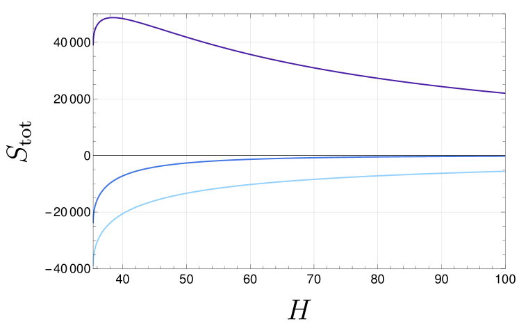
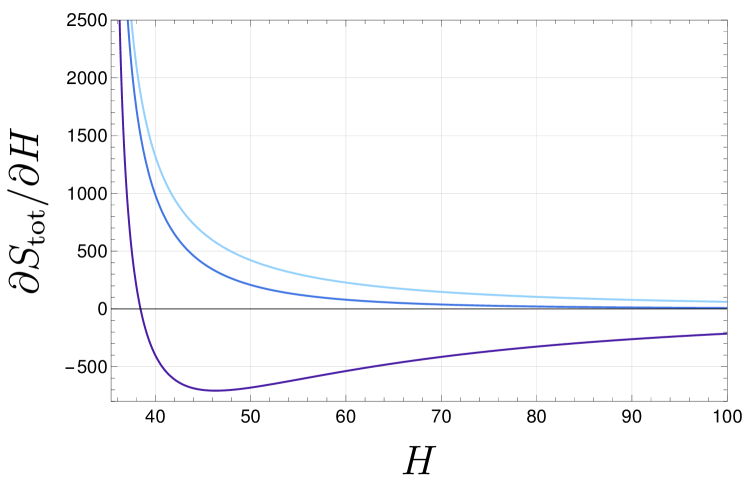
Figure 7: Total Regge action (left) and its derivative (right) for a single slice with boundary data $s_{0}=50,s_{1}=100$ and scalar field differences $\Delta\phi_{*}-2$ (light blue), $\Delta\phi_{*}$ and $\Delta\phi_{*}+2$ (dark blue). Here, we set $\lambda=8\pi G_{\mathrm{N}}=1$ such that the limiting value of Eq. (54) is given by $\Delta\phi_{*}=2\sqrt{\frac{2}{3}}$. For $\Delta\phi<\Delta\phi_{*}$ there is no solution to the equation of motion, while for $\Delta\phi>\Delta\phi_{*}$ there exists a solution.

For more than two spatial slices, say $M+1$, non-trivial equations for bulk spatial length $\{s_{n}\}$ and scalar field values $\{\phi_{n}\}$ must be satisfied. As for the case of $M=1$, the equations for the height variables $\{H_{n}\}$ exhibit solutions, provided that the inequality of Eq. (54) holds on every slice. Notice that these conditions now also affect bulk spatial lengths and scalar field values. That is, the equations of motion for the $\{H_{n}\}$ constrain the equations of bulk spatial edge lengths and scalar fields.

Assuming that the equation $\partial S_{\mathrm{tot}}/\partial H_{n}=0$ is satisfied, i.e. Eq. (50a) holds, we extract

$$\frac{\pi}{2}-\cos^{-1}\left(\frac{\Delta s_{n}^{2}}{4H_{n}^{2}-\Delta s_{n}^{2}}\right)=-\left(\partialderivative{\absolutevalue{k_{n}}}{H_{n}}\right)^{-1}\partialderivative{S_{\phi}^{(n)}}{H_{n}}.$$ (55)

Implicitly, the height variables $\{H_{n}\}$ are therefore given as functions of the spatial edge length and the scalar field variables, i.e. $H_{n}=H_{n}(\{s_{m}\},\{\phi_{m}\})$. As a result, the equation for spatial edge length $s_{n}$, explicitly given in Eq. (50b), reduces to

$$\sinh^{-1}\left(\frac{s_{n}-s_{n-1}}{\sqrt{4H_{n-1}^{2}-(s_{n}-s_{n-1})^{2}}}\right)=\sinh^{-1}\left(\frac{s_{n+1}-s_{n}}{\sqrt{4H_{n}^{2}-(s_{n+1}-s_{n})^{2}}}\right).$$ (56)

We used the equation

$$\partialderivative{\absolutevalue{k_{n}}}{s_{n}}\left(\partialderivative{\absolutevalue{k_{n}}}{H_{n}}\right)^{-1}\partialderivative{S_{\phi}^{(n)}}{H_{n}}=\partialderivative{S_{\phi}^{(n)}}{s_{n}},$$ (57)

which holds by chain rule and applies if the functions are invertible. This is the case if we exclude lightlike trapezoids for which $k_{n}$ vanishes, i.e. we demand that $H_{n}^{2}\neq\frac{1}{2}\Delta s_{n}^{2}$.

Finally, Eq. (56) implies that

$$\frac{s_{n+1}-s_{n}}{H_{n}}=\frac{s_{n}-s_{n-1}}{H_{n_{1}}}.$$ (58)

This means that relative to the $4$-height, the differences of spatial edge lengths within a $4$-frustum remain constant along the entire discrete spacetime.

Solving for $s_{n}$, we find

$$s_{n}=\frac{s_{n-1}H_{n}+s_{n+1}H_{n}}{H_{n-1}+H_{n-1}},$$ (59)

where we notice the structural similarities compared to the scalar field equation (34). Given boundary data $(s_{0},s_{M})$, and introducing the sum of $4$-heights between slice $m_{1}$ and $m_{2}$,

$$\mathcal{H}_{m_{1}}^{m_{2}}=\sum_{m=m_{1}}^{m_{2}}H_{m}$$ (60)

the $n$-th spatial edge length is given by

$$s_{n}=\frac{s_{M}\mathcal{H}_{0}^{n-1}+s_{0}\mathcal{H}_{n}^{M-1}}{\mathcal{H}_{0}^{M-1}}.$$ (61)

Notice that the scalar field dependence of the spatial edge length $s_{n}$ enters via the height variables $\{H_{n}\}$.

With these formulas, the differences of neighbouring spatial length, say on slice $n+1$ and $n$ is expressed as

$$\frac{s_{n+1}-s_{n}}{H_{n}}=\frac{s_{M}-s_{0}}{\mathcal{H}_{0}^{M-1}}.$$ (62)

That is, the length difference of spacelike edges relative to the height of a given $4$-frustum is the same as the length difference of the boundary spacelike edges, $(s_{M}-s_{0})$ relative to the total height $\mathcal{H}_{0}^{M-1}$. Importantly, from this equation it follows that the spatial edge length evolve monotonically, with the sign determined by relation of $s_{M}$ and $s_{0}$, i.e.

$$\mathrm{sgn}(s_{n+1}-s_{n})=\mathrm{sgn}(s_{M}-s_{0}),\qquad\forall n\in\{0,...,M-1\}.$$ (63)

Consequently, the boundary data selects either the contracting or expanding branch, similar to what is found in the continuum, see Appendix B.

4.3 Linearisation, deparametrisation and continuum limit

The discussion on the solutions of the Regge equations has been mostly qualitative so far. To obtain a more quantitative understanding, we consider in this section the expansion of the Regge equations around small deficit angles of both types, i.e. $\varphi_{nn+1}\ll 1$ and $\theta_{n}\ll 1$. This procedure will reduce the transcendental equations to polynomial ones.

Both types of deficit angles are a function of

$$\eta_{n}=\frac{s_{n+1}-s_{n}}{H_{n}}.$$ (64)

Clearly, expanding in small $\eta_{n}$ yields an expansion in small deficit angles with the flat case given by $s_{n}=s_{n+1}$, i.e. $\eta_{n}=0$. Notice also that in order to remain within the causally regular sector, $\eta_{n}$ must obey the bound $\eta_{n}^{2}<2$. An expansion of the equation $\partial S/\partial H_{n}=0$ around $\eta_{n}=0$ yields

$$6(s_{n}+s_{n+1})\left(\frac{\eta_{n}^{2}}{4}+\frac{\eta_{n}^{4}}{8}+\mathcal{O}(\eta_{n}^{6})\right)-\lambda 8\pi G_{\mathrm{N}}\frac{(s_{n}+s_{n+1})^{3}}{16H_{n}^{2}}(\phi_{n+1}-\phi_{n})^{2}=0.$$ (65)

As a consistency check, we notice that cutting the equation at vanishing order of $\eta_{n}$ yields the flat solution where $\Delta s_{n}=0$ and $\Delta\phi_{n}=0$ for all slices $n$.

At first non-vanishing order, $\eta_{n}$ enters Eq. (65) quadratically and the dependence on the height variable $H_{n}$ drops out, yielding

$$\left(\frac{2}{s_{n}+s_{n+1}}\right)^{2}\left(\frac{s_{n+1}-s_{n}}{\phi_{n+1}-\phi_{n}}\right)^{2}=\lambda\frac{4\pi G_{\mathrm{N}}}{3},$$ (66)

which corresponds exactly yo the limiting case of the inequality (54). This equation is relational in the sense that it only involves the spatial edge length and the scalar field values, independent of the height of the frusta. In fact, one can show that the $H_{n}$ are undetermined at this level of expansion by the whole system of equations, similar to the vacuum case of Sec. 4.1. It is at this level of expansion, where one can define a continuum time limit, which we discuss in the following paragraph.

Continuum time limit.

Defining a continuum limit for the general Regge action is a challenging task. However, in the symmetry reduced model we are considering here, the system is effectively one-dimensional with non-trivial dynamics in temporal direction. Schematically speaking, the continuum limit corresponds to infinitesimally small but many time steps, at each of which the deficit angles are small Bahr:2017bn ; Brewin1999 . Consequently, this limit is two-fold. First, as performed for the scalar field in Sec. 3.3, the height of a $4$-frustum is interpreted as finite proper time which, in the continuum limit, is mapped to $H_{n}\rightarrow\differential{\tau}=N\differential{t}$. Spatial edge lengths $\{s_{n}\}$ and scalar field values $\{\phi_{n}\}$ are mapped according to Eqs. (40) and (41), respectively. The second limit needed to recover the Friedmann equations is that of small deficit angles which has been performed above as an expansion in the parameter $\eta_{n}$. Following this prescription, we start with Eq. (66) and find at vanishing order of $\differential{t}$

$$\left(\frac{\dot{a}}{a}\right)^{2}=\lambda\frac{4\pi G_{\mathrm{N}}}{3}\dot{\phi}^{2},$$ (67)

corresponding indeed the continuum Friedmann equation.

Given the already relational form of Eq. (66), introducing an artificial time parameter $t$ with lapse $N$ is actually not necessary. Instead, we consider the continuum limit $\phi_{n+1}-\phi_{n}\rightarrow\differential{\phi}$ (which implicitly assumes the scalar field differences to be approximately constant along the slices) and understand the spatial length variables as functions of the relational clock $\phi$, yielding

$$s_{n}\rightarrow a(\phi),\qquad s_{n\pm 1}\rightarrow a(\phi)\pm a^{\prime}(\phi)\differential{\phi}+\frac{1}{2}a^{\prime\prime}(\phi)\differential{\phi}^{2},$$ (68)

where prime denotes the derivative with respect to the scalar field. Then, at vanishing order of $\differential{\phi}$, Eq. (66) becomes

$$\left(\frac{a^{\prime}}{a}\right)^{2}=\lambda\frac{4\pi G_{\mathrm{N}}}{3},$$ (69)

corresponding to the relational continuum Friedmann equation.

Since in the continuum the lapse function corresponds to a gauge redundancy, the set of equations after deparametrisation should be in fact smaller than in the discrete, where the variable $H_{n}$ is in fact dynamical. This reduction of independent equations can be seen from the non-perturbative (i.e. at all order in $\eta_{n}$) equation (58). Clearly, in the continuum time limit as prescribed by Eqs. (40) and (41), Equation (58) takes the form $\dot{a}=\dot{a}$ which becomes trivially satisfied.

In the discrete, Eq. (66) can be solved explicitly for one of the edge length, say $s_{n+1}$. Solving the polynomial of second degree, we obtain

$$s_{n+1}^{+}=\frac{1+\sqrt{\lambda\frac{\pi G_{\mathrm{N}}}{3}(\phi_{n+1}-\phi_{n})^{2}}}{\absolutevalue{1-\sqrt{\lambda\frac{\pi G_{\mathrm{N}}}{3}(\phi_{n+1}-\phi_{n})^{2}}}}s_{n},\qquad s_{n+1}^{-}=\frac{\absolutevalue{1-\sqrt{\lambda\frac{\pi G_{\mathrm{N}}}{3}(\phi_{n+1}-\phi_{n})^{2}}}}{1+\sqrt{\lambda\frac{\pi G_{\mathrm{N}}}{3}(\phi_{n+1}-\phi_{n})^{2}}}s_{n},$$ (70)

corresponding to the expanding and contracting solutions, respectively. Since this relation can be derived for any slice, and since Eq. (63) dictates global monotonicity, we find a relation between distant slices by iteration,

$$s_{M}^{\pm}=\prod_{n=0}^{M-1}\kappa^{\pm}_{n}s_{0},$$ (71)

where $\kappa^{\pm}_{n}$ are the defining coefficients of Eq. (70). Approximating the scalar field differences as $\phi_{n+1}-\phi_{n}=(\phi_{M}-\phi_{0})/M$ and using the limit definition of the exponential function, $\lim_{n\rightarrow\infty}(1+x/n)^{n}=\mathrm{e}^{x}$, we find

$$\lim\limits_{M\rightarrow\infty}s_{M}^{\pm}=s_{0}\exp\left(\pm\sqrt{\lambda\frac{4\pi G_{\mathrm{N}}}{3}}(\phi_{M}-\phi_{0})\right),$$ (72)

which corresponds indeed to the relational continuum solution of Eq. (87).

Higher orders.

Including higher orders of the parameter $\eta_{n}$ to the full system of equations increases in general the degree of the resulting polynomial equations. Already at fourth order in $\eta_{n}$, the equation $\partial S/\partial H_{n}=0$ shows qualitative differences compared to the lowest order case. In particular, the equation becomes explicitly dependent on the height variable $H_{n}$, for which one can solve explicitly

$$H_{n}^{2}=\frac{\frac{1}{2}\Delta s_{n}^{4}}{\lambda\frac{4\pi G_{\mathrm{N}}}{3}\left(\frac{s_{n}+s_{n+1}}{2}\right)^{2}\Delta\phi_{n}^{2}-\Delta s_{n}^{2}}.$$ (73)

Here, we see explicitly that the inequality (54) is required to hold in order to yield a real Lorentzian height $H_{n}\in\mathbb{R}$. Going to even higher orders in $\eta_{n}$, one can show that this inequality in fact permeates all orders.

Causality violations and continuum limit.

Only causally regular terms admit an expansion in terms of small parameters $\eta_{n}$ defined in Eq. (64). That is because causality violating terms are given for $\eta_{n}^{2}>2$ and therefore, an expansion for $\eta_{n}\ll 1$ is not justified. Following the construction of the continuum limit, such configurations therefore do not admit a limit of $H_{n}\rightarrow N\differential{t}$ and simultaneously taking the deficit angles to be small. In the present symmetry reduced setting, this suggests that causality violations are a feature of the discrete theory that are not visible in an appropriate continuum limit. A more general result on the interplay of discreteness and causal structure remains however an open question.

4.4 Classical equations and causality violations

In the preceding three sections, we focused on the Regge equations of (hinge) causally regular configurations satisfying the inequality $H_{n}^{2}>\frac{1}{2}(s_{n}-s_{n+1})^{2}$. There, the Regge action is real such that the number of real equations equals the number of real dynamical variables. Hence the analysis has been performed in a standard way. However, if hinge causality violations are present, the Regge action is complex, therefore leading to complex equations of motion for a priori real dynamical variables. We discuss in the following how such types of systems can be studied along the lines of Asante:2021phx .

Complex actions for gravity have been studied in the context of the Euclidean gravity path integral Louko:1995jw ; Gibbons:1976ue ; Gibbons:1978ac ; Witten:2021nzp , continuum Lorentzian quantum cosmology Feldbrugge:2017kzv , semi-classical analyses of Lorentzian spin foams Han:2020npv ; Han:2023cen ; Han:2021kll as well as Lorentzian effective spin foams Asante:2021phx ; Asante:2021zzh . Therein, the path integral over real metric configurations is replaced by a complex line integral over a contour $C$ in the space of complex metrics, formally written as

$$Z=\int_{C}\mathcal{D}g\mathrm{e}^{\frac{1}{\hbar}\mathcal{S}[g]},$$ (74)

where $\mathcal{S}[g]$ is an analytic functional of the complex metric $g$. Choosing the contour to be a Lefshetz-thimble Lefshetz1975 ; Vassiliev2002 , i.e. a path of steepest descent that passes through one or more critical points $g_{0}$, the convergence of the integral improves significantly. For explicit examples in the setting of discrete and continuum quantum cosmology, see Asante:2021phx and Feldbrugge:2017kzv , respectively. In an asymptotic expansion $\hbar\rightarrow 0$, the saddle points $g_{0}$ dominate the path integral. Therefore, as in standard quantum mechanics, the saddle points of the action can be interpreted as the classical (however complex) configurations.

Applied to the present setting of complex Regge actions, we conclude that a complexification of the variables is necessary to obtain an equal number of equations and dynamical variables. Given two slices, i.e. $M=1$, the only dynamical variable is the squared height $H^{2}=R^{2}\mathrm{e}^{i\alpha}$ for which the corresponding analytic actions $\mathcal{S}(R,\alpha)$ have been discussed in Sec. 2.5. For $M>1$, the spatial edge lengths in the bulk also become dynamical, necessitating further complexification and analytic continuation. In the following, we restrict ourselves to the case of $M=1$.

In Sector III, the total complex action $\mathcal{S}_{\mathrm{III}}^{\mathrm{tot}}$ has saddle points either on Lorentzian data, $\alpha=\pm\pi$, or on Euclidean data, $\alpha=0,2\pi$, depending on the boundary data. More precisely, if Eq. (54) is satisfied, there are Lorentzian solutions. If Eq. (54) is violated, then there are Euclidean solutions given at $\alpha=0,2\pi$. Both solutions require that $\lambda>0$.

Sectors I and II include hinge causality violations and are described by the complex actions $\mathcal{S}^{\mathrm{tot}}_{\mathrm{I}}$ and $\mathcal{S}^{\mathrm{tot}}_{\mathrm{II}}$, respectively. Their limiting values $\alpha\rightarrow\pm\pi$ and $\alpha\rightarrow 0,2\pi$ are summarised in Eqs. (27)–(29). From these limiting values, consider for instance the Lorentzian action $S_{\mathrm{tot}}^{\mathrm{L},+}$. Its derivative with respect to the radial variable $R$ is depicted in Fig. 8. We observe that for certain boundary data $(s_{0},\phi_{0})$ and $(s_{1},\phi_{1})$, the real part (drawn in solid blue) exhibits a saddle point with respect to the radial variable $R$ given that $\lambda<0$. However, the imaginary part (drawn in dashed red) is never zero, in particular not at the zeroes of the real part. As a consequence, the causality violating sectors do not exhibit saddle points on the Lorentzian lines $(R,\alpha)=(R,\pm\pi)$. We therefore conclude that there are no classical solutions for the Lorentzian action with causality violations.

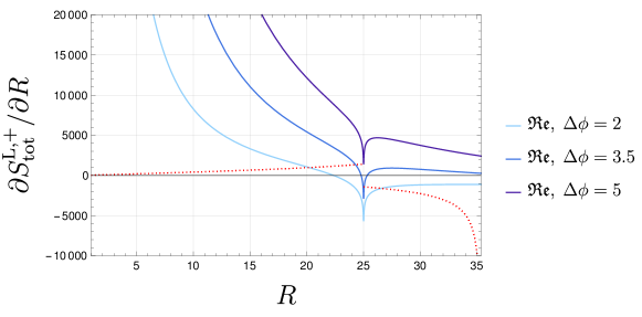
Figure 8: Real (solid blue) and imaginary (dashed red) parts of the derivative of the total Regge action in Sectors I and II with the choice of convention “$+$”. Boundary data is given by $s_{0}=50,s_{1}=100$ and parameter values $\lambda=-1$ and $8\pi G_{\mathrm{N}}=1$ are chosen. Although the real part shows saddle points for certain values of $\Delta\phi$, the imaginary part is nowhere vanishing.

Similarly, there are no saddle points on Euclidean lines $(R,0)$ and $(R,2\pi)$ for causality violating data, where $R^{2}<\frac{1}{4}\Delta s^{2}$ in Sector I and $\frac{1}{4}\Delta s^{2}<R^{2}<\frac{1}{2}\Delta s^{2}$ in Sector II. Expressions of the action on these lines are given in Eqs. (29).

These results suggest, that there is no classical correspondence for causality violating terms in the Euclidean or Lorentzian sector. Consequently, such configurations are treated purely quantum, and are only taken into account in a path integral. There is still the possibility, that the actions $\mathcal{S}^{\mathrm{tot}}_{\mathrm{I}}$ and $\mathcal{S}^{\mathrm{tot}}_{\mathrm{II}}$ have saddle points in the fully complex regime, i.e. when $\alpha$ is not given by $0,2\pi$ or $\pm\pi$. Results of Asante:2021phx indicate that also for other angles $\alpha$, no saddle points exist. Given that in this work, the parameter $\lambda$ can in principle be also negative, it is however unclear if these results can be transferred to the setting here. In particular, complex solutions might require $\lambda<0$, on the interpretation of which we comment below.

A comment on energy conditions.

The Regge equation for a single slice exhibits a causally regular solution, either Lorentzian or Euclidean, if the coupling parameter $\lambda$ of the matter term in Eq. (32) is positive. As discussed above, Sectors I and II possibly exhibit complex solutions that require $\lambda$ to be negative. In this case, an analogy to the continuum could be drawn, where the sign of $\lambda$ corresponds to the sign of the energy density, given by the $(00)$-component of the energy-momentum tensor. The case of $\lambda>0$ yields an energy-momentum tensor that satisfies the strong energy condition HawkingBook , which has been shown in Tipler:1977eb to guarantee a causally regular structure without singularities. If the strong energy condition is violated, which in this case would correspond to $\lambda<0$, causality violations cannot be excluded. These continuum results are exemplary for the intimate relation between matter and the causal structure and possibly translate to the present discrete setting. Further investigation in this direction is left open as an interesting future avenue.

5 Discussion and conclusion

The purpose of this article was to develop and study the classical discrete theory for spatially flat, homogeneous and isotropic cosmology within the framework of Lorentzian Regge calculus. As matter content of the universe, we investigated a minimally coupled massless free scalar field which is commonly employed in quantum cosmology to serve as a relational clock. A firm understanding of the kinematics and dynamics of the coupled system serves as a foundation for future investigations of the symmetry restricted path integral in the spirit of effective spin foams Asante:2020qpa ; Asante:2020iwm ; Asante:2021zzh ; Dittrich:2023rcr .

Starting from a triangulation that allows the split into triangulated spacelike hypersurfaces we imposed spatial homogeneity and isotropy. Together with the requirement of spatial flatness, we obtained a discretisation consisting of $4$-dimensional frusta that are internally triangulated in a flat way. In Secs. 2.1–2.3, we derived the corresponding Lorentzian Regge action and its geometrical ingredients as a function of the edge length of cubes and the $4$-heights of frusta. We examined in Sec. 2.4 the different sectors of the theory, summarised in Fig. 3, with regard to their causality properties. Notably, causality violations, as introduced in Asante:2021phx , are present if edges, trapezoids or $3$-frusta between slices are spacelike. A Wick rotation to the Euclidean sector can be defined by complexifying the height variables and analytically continuing the action. As we discussed in Sec. 2.5 this requires particular care in the presence of hinge causality violations.

We introduced a minimally coupled massless free scalar field to the discrete cosmological model in Sec. 3, studied its equations of motion and showed that solutions evolve monotonically as dictated by the boundary data. Moreover, it is straightforward to define a continuum limit of the scalar field equations, which we showed in Sec. 3.3 to agree with the continuum equations given in Appendix B.

In accordance with the continuum, the vacuum Regge equations exhibit only static solutions where the spacelike geometric data remains constant along discrete temporal evolution. Indeterminacy of the $4$-height is in this case reminiscent of a restoration of diffeomorphism symmetry which, in the cosmological setting, is reflected in the lapse function $N$ being a gauge redundancy. In the presence of a non-vanishing scalar field, the causally regular Regge equations for the height variables exhibit solutions if the inequality (54) is satisfied. Furthermore, we extracted from the full equations of motion that the spacelike edge lengths evolve monotonically, constituting a contracting or an expanding branch. In Sec. 4.3 we studied a small deficit angle expansion of the transcendental Regge equations. At lowest non-vanishing order, the dependence on the height variable drops out similar to the vacuum case. This marks the level at which the system deparametrises and the evolution of spatial geometric data is described in a relational sense with respect to the scalar field. Moreover, a continuum limit at this level of truncation yields the correct relational Friedmann equations. Taking higher orders into account, the height variables become dynamical, obstructing a deparametrisation of the system. Lastly in Sec. 4.4 we discussed the existence and characterisation of classical solutions in the presence of causality violations.

From our investigation of this cosmological model, we can draw a few tentative conclusions. We observe that causality violations generically appear if the building blocks connecting spatial slices are spacelike. This applies in particular to the situation in which the 3-frusta and trapezoids are entirely spacelike. For these sectors of the theory no solutions exist, at least for real length variables, and the entirely timelike sector appears preferred both in vacuum and in the presence of a massless scalar field. This casts doubts on the viability to describe cosmology in such a symmetry reduced setting with entirely spacelike 3d building blocks, as prescribed by the Lorentzian EPRL model. However, this is not conclusive from our analysis, as the symmetry reduction used here is highly restrictive. It is conceivable that these issues can be circumvented by deviating from homogeneity and isotropy and that these notions could reappear (effectively) after coarse graining or averaging. Nevertheless, recent works in group field cosmology Jercher:2023nxa ; Jercher:2023kfr suggest that timelike polyhedra need to be included to obtain GR-like perturbations.

The simple cosmological model described in this article provides a possibility to study the refinement limit in the quantum theory, similar to the Euclidean considerations Bahr:2018gwf . On the one hand, we can study bulk refinements by adding more time steps to the triangulation. On the other hand, we can refine the boundary. While the former adds additional degrees of freedom, the latter does not due to the strong symmetry restrictions. Thus, this setting can give first insights into the definition of a continuum limit. Once the symmetries, i.e. homogeneity and isotropy, are eventually lifted, more interesting scenarios can be explored. For example, one can conceive a triangulation in which different spatial slices have a different number of faces and edges. Thus, under evolution degrees of freedom are added or removed with the spin foam acting as a dynamical embedding map relating states in different Hilbert spaces. See Dittrich:2009fb ; Dittrich:2011ke and Dittrich:2013xwa ; Hohn:2014uvt ; Hohn:2014rba for the exploration of these ideas in Regge calculus and path integrals respectively. Such a procedure might help to address the question whether an effective cosmological dynamics emerges from the full theory via coarse graining.

We close this work by listing intriguing questions that wait to be addressed by the path integral quantisation of the model developed here.

• Transfer matrix method: The slicing structure of the action possibly allows to cast the system in a transfer matrix formalism and study the properties of the transition amplitudes similar to Causal Dynamical Triangulations Ambjorn:2012pp ; Ambjorn:2014mra .

• Boundary states and semi-classics: It will be interesting to study the definition of suitable boundary states that are peaked on the scale factor and under which conditions semi-classical physics are recovered from the quantum theory. Our present analysis of the classical dynamics will be crucial in this task.

• Acceleration operators: Evaluating the effective Lorentzian spin foam sum is computationally challenging even in a strongly symmetry restricted model as the one developed here. That is due to the oscillatory nature of the effective spin foam amplitudes of the form $\mathrm{e}^{iS_{\mathrm{R}}}$. The recently re-discovered acceleration operators might prove highly useful to improve convergence Dittrich:2023rcr . Including causally irregular configurations and comparing to the spatially spherical model Dittrich:2023rcr will be interesting to study as well.

• Quantum bounce: Studying the existence of a quantum bounce in effective spin foams is expected to be insightful for the mechanism of such bouncing scenarios. In particular, this might answer if semi-classical amplitudes together with discrete area spectra are sufficient for a singularity resolution.

• Deparametrisation: Beyond the vacuum theory, the interplay between geometry and the massless scalar field is intriguing. In particular, the question arises whether the theory can be deparametrised and under which conditions this is possible. We have already observed that classically, reparametrisation invariance gets restored in a continuum limit, in which the deficit angles are small. This is consistent, as we expect a restoration of continuum symmetries in a suitable refinement limit, see e.g. the recent review Asante:2022dnj . Still, conceptual questions remain, e.g. with respect to which observable to deparametrise and whether this idea might be spoiled by fluctuations of matter and gravity.

Acknowledgements

The authors are grateful to Seth Asante, Markus Schröfl, Luca Marchetti, Daniele Oriti and Steffen Gielen for helpful comments and discussions. AFJ and SSt gratefully acknowledge support by the Deutsche Forschungsgemeinschaft (DFG, German Research Foundation) project number 422809950. AFJ kindly acknowledges support from the MCQST via the seed funding Aost 862983-4 and from the Deutsche Forschungsgemeinschaft (DFG) under Grant No 406116891 within the Research Training Group RTG 2522/1.

Appendix A Lorentzian dihedral angles of $4$-frusta

In this appendix we derive the dihedral angles for the Lorentzian $4$-frustum following the conventions of Sorkin:2019llw ; Asante:2021zzh . In the boundary of a $4$-frustum there are three distinct $3$-dimensional building blocks, being the initial and final cube as well as the six boundary $3$-frusta. Due to homogeneity and isotropy, there are three distinct dihedral angles per slab $(n,n+1)$, being $\varphi_{nn+1}$, $\varphi_{n+1n}$ and $\theta_{n}$ located at the initial and final square and the trapezoids, respectively.

We compute these angles by embedding a single $4$-frustum in flat Minkowski space $\mathbb{R}^{1,3}$ and determining the outward-pointing normal vectors of the $3$-dimensional building blocks. For initial and final cube, these are respectively given by $N_{s,\mp}=(\mp 1,0,0,0)$. To obtain normal vectors of the $3$-frusta, we form the wedge product of three spanning vectors and act with the Hodge-star operator $*$. As a result, the six normal vectors are given by

$$N_{\pm,i}=\frac{1}{\sqrt{\absolutevalue{H_{n}^{2}-\left(\frac{s_{n}-s_{n+1}}{2}\right)^{2}}}}\left(\frac{s_{n}-s_{n+1}}{2},\pm H_{n}{\bf\it e}_{i}\right).$$ (75)

The signature of $N_{\pm,i}$ is opposite of the signature of the $3$-frustum, i.e. $\eta(N_{\pm,i},N_{\pm,i})=-1$ for the $3$-frustum to be spacelike and $\eta(N_{\pm,i},N_{\pm,i})=1$ for the $3$-frustum to be timelike. Notice that the time orientation for a timelike normal vector depends on whether $s_{n}<s_{n+1}$ or vice versa.

Lorentzian dihedral angles are defined in terms of the Minkowski product of the normal vectors associated to the two polyhedra. For the three cases we consider here, these are given by

$$\eta(N_{\pm i},N_{\pm j}) =-\frac{(s_{n}-s_{n+1})^{2}}{\absolutevalue{4H_{n}^{2}-(s_{n}-s_{n+1})^{2}}},$$ (76)

$$\eta(N_{\pm,i},N_{s,\mp}) =\pm\frac{s_{n}-s_{n+1}}{\sqrt{\absolutevalue{4H_{n}^{2}-(s_{n}-s_{n+1})^{2}}}}.$$ (77)

The precise form of the Lorentzian angles $\varphi_{nn+1},\varphi_{n+1n}$ and $\theta_{n}$ as a function of the Minkowski products depend then on the signature of the $3$-polyhedra. Moreover, the signature of the trapezoid is decisive for the associated angle to be either Lorentzian or Euclidean. With the conventions of Sorkin:2019llw ; Asante:2021zzh , the angles in Eqs. (9)–(12) follow.

Appendix B Relational cosmology in the continuum

Here, we briefly summarise the equations of spatially flat cosmology with a minimally coupled massless scalar field, first in coordinates and then in a relational manner. The resulting formulae serve as a comparison for the continuum limit of the Regge equations, studied in Sec. 4.3.

B.1 Spatially flat cosmology and the lapse function

As the starting point, we consider the spatially flat FLRW-metric, defined by the line element

$$\differential{s}^{2}=g_{\mu\nu}\differential{x}^{\mu}\differential{x}^{\nu}=-N^{2}\differential{t}^{2}+a^{2}\differential{{\bf\it x}}^{2},$$ (78)

where $N$ is the Lapse function, $a$ is the scale factor and $\differential{{\bf\it x}}^{2}$ is the line element of flat $3$-dimensional Euclidean space. The corresponding symmetry reduced Einstein-Hilbert action is given by

$$S_{\mathrm{EH}}[a,N]=\frac{3}{8\pi G_{\mathrm{N}}}\int\differential{t}\frac{a^{3}}{N}\left(\frac{\ddot{a}}{a}-\frac{\dot{N}}{N}\frac{\dot{a}}{a}+\left(\frac{\dot{a}}{a}\right)^{2}+N^{2}\frac{k}{a^{2}}\right).$$ (79)

As matter content, we consider a minimally coupled massless scalar field, the action of which is given by

$$S_{\phi}[a,N,\phi]=\frac{\lambda}{2}\int\differential{t}\frac{a^{3}}{N}\dot{\phi}^{2},$$ (80)

yielding

$$\derivative{t}\left(\frac{a^{3}}{N}\dot{\phi}\right)=0$$ (81)

as equation of motion.

Variation of the total action $S_{\mathrm{tot}}=S_{\mathrm{EH}}+S_{\phi}$ with respect to the lapse function $N$ yields the first Friedmann equation

$$\left(\frac{\dot{a}}{a}\right)^{2}+N^{2}\frac{k}{a^{2}}=\lambda\frac{4\pi G_{\mathrm{N}}}{3}\dot{\phi}^{2},$$ (82)

while the variation with respect to the scale factor $a$ yields the second Friedmann equation

$$2\frac{\ddot{a}}{a}-2\frac{\dot{N}}{N}\frac{\dot{a}}{a}+\left(\frac{\dot{a}}{a}\right)^{2}+N^{2}\frac{k}{a^{2}}=-\lambda 4\pi G_{\mathrm{N}}\dot{\phi}^{2}.$$ (83)

Altogether, Eqs. (81), (82) and (83) form a set of two independent equations with the third equation being redundant. These two equations determine the dynamics of the physical variables $a$ and $\phi$.

Notice that under a complexification of the lapse function $N\rightarrow iN_{\mathrm{E}}$ to Euclidean signature, the two Friedmann equations stay invariant if $k=0$, i.e. in the spatially flat case.

B.2 Deparametrisation in the continuum

Following the relational strategy Rovelli:1990ph ; Dittrich:2005kc ; Hoehn:2019fsy , the dependence of the Friedmann equations on the lapse function $N$ and the unphysical time coordinate $t$ can be removed by deparametrising the system with respect to the scalar field $\phi$, thus serving as a relational clock. To that end, the scalar field is assumed to be on-shell, i.e.

$$\derivative{\phi}{t}=\frac{cN}{a^{3}},$$ (84)

where $c$ is the integration constant arising from solving Eq. (81).

Then, the two Friedmann equations (82) and (83) can be deparametrised, yielding

$$\left(\frac{a^{\prime}}{a}\right)^{2}+\frac{a^{4}}{c^{2}}k =\lambda\frac{4\pi G_{\mathrm{N}}}{3},$$ (85)

$$2\frac{a^{\prime\prime}}{a}-5\left(\frac{a^{\prime}}{a}\right)^{2}+\frac{a^{4}}{c^{2}}k =-\lambda 4\pi G_{\mathrm{N}}.$$ (86)

Notice that the second equation is a derivative of the first and hence dependent, because the scalar field equation has been imposed to deparametrise the system. As expected, the lapse function $N$ as well as the coordinate time $t$ vanished from the formalism completely with only the scale factor $a(\phi)$ as a function of the physical clock $\phi$ remaining.

For initial conditions $a(\phi_{0})=a_{0}$ and in the standard case of $\lambda=1$, the two solutions of this equation in the spatially flat case ($k=0$) are given by

$$a(\phi)=a_{0}\exp\left({\pm\sqrt{\frac{4\pi G_{\mathrm{N}}}{3}}(\phi-\phi_{0})}\right),$$ (87)

where $\pm$ leads to the expanding, respectively the contracting branch of solutions.

References

- (1) Planck collaboration, Planck 2018 results. VI. Cosmological parameters, Astron. Astrophys. 641 (2020) A6 [1807.06209].
- (2) A. Pérez, The Spin-Foam Approach to Quantum Gravity, Living Rev. Relativity 16 (2013) 3 [1205.2019].
- (3) A. Ashtekar and E. Bianchi, A short review of loop quantum gravity, Rept. Prog. Phys. 84 (2021) 042001 [2104.04394].
- (4) D. Oriti, The group field theory approach to quantum gravity, in Approaches to Quantum Gravity: Toward a New Understanding of Space, Time and Matter, D. Oriti, ed., (Cambridge, UK), Cambridge University Press (2007) [gr-qc/0607032].
- (5) L. Freidel, Group field theory: An Overview, Int. J. Theor. Phys. 44 (2005) 1769 [hep-th/0505016].
- (6) L. Marchetti and D. Oriti, Effective relational cosmological dynamics from Quantum Gravity, JHEP 05 (2021) 025 [2008.02774].
- (7) D. Oriti, L. Sindoni and E. Wilson-Ewing, Emergent Friedmann dynamics with a quantum bounce from quantum gravity condensates, Class. Quant. Grav. 33 (2016) 224001 [1602.05881].
- (8) S. Gielen and L. Sindoni, Quantum Cosmology from Group Field Theory Condensates: a Review, SIGMA 12 (2016) 082 [1602.08104].
- (9) A.F. Jercher, D. Oriti and A.G.A. Pithis, Emergent cosmology from quantum gravity in the Lorentzian Barrett-Crane tensorial group field theory model, JCAP 01 (2022) 050 [2112.00091].
- (10) I. Agullo and P. Singh, Loop Quantum Cosmology, in Loop Quantum Gravity: The First 30 Years, A. Ashtekar and J. Pullin, eds., pp. 183–240, WSP (2017), DOI [1612.01236].
- (11) B. Bahr, S. Klöser and G. Rabuffo, Towards a Cosmological subsector of Spin Foam Quantum Gravity, Phys. Rev. D 96 (2017) 086009 [1704.03691].
- (12) E. Bianchi, C. Rovelli and F. Vidotto, Towards spinfoam cosmology, Phys. Rev. D 82 (2010) 084035 [1003.3483].
- (13) C. Rovelli, What Is Observable in Classical and Quantum Gravity?, Class. Quant. Grav. 8 (1991) 297.
- (14) C. Rovelli, Partial observables, Phys. Rev. D 65 (2002) 124013 [gr-qc/0110035].
- (15) B. Dittrich, Partial and complete observables for canonical general relativity, Class. Quant. Grav. 23 (2006) 6155 [gr-qc/0507106].
- (16) P.A. Hoehn, A.R.H. Smith and M.P.E. Lock, Trinity of relational quantum dynamics, Phys. Rev. D 104 (2021) 066001 [1912.00033].
- (17) E. Bianchi, T. Krajewski, C. Rovelli and F. Vidotto, Cosmological constant in spinfoam cosmology, Phys. Rev. D 83 (2011) 104015 [1101.4049].
- (18) J. Rennert and D. Sloan, A Homogeneous Model of Spinfoam Cosmology, Class. Quant. Grav. 30 (2013) 235019 [1304.6688].
- (19) G. Sarno, S. Speziale and G.V. Stagno, 2-vertex Lorentzian Spin Foam Amplitudes for Dipole Transitions, Gen. Rel. Grav. 50 (2018) 43 [1801.03771].
- (20) J. Engle, R. Pereira and C. Rovelli, Loop-Quantum-Gravity Vertex Amplitude, Phys. Rev. Lett. 99 (2007) 161301 [0705.2388].
- (21) J. Engle, E.R. Livine, R. Pereira and C. Rovelli, LQG vertex with finite Immirzi parameter, Nucl. Phys. B 799 (2008) 136 [0711.0146].
- (22) F. Gozzini and F. Vidotto, Primordial Fluctuations From Quantum Gravity, Front. Astron. Astrophys. Cosmol. 7 (2021) 629466 [1906.02211].
- (23) P. Frisoni, F. Gozzini and F. Vidotto, Markov chain Monte Carlo methods for graph refinement in spinfoam cosmology, Class. Quant. Grav. 40 (2023) 105001 [2207.02881].
- (24) P. Frisoni, F. Gozzini and F. Vidotto, Primordial fluctuations from quantum gravity: 16-cell topological model, 2312.02399.
- (25) B. Bahr and S. Steinhaus, Investigation of the Spinfoam Path integral with Quantum Cuboid Intertwiners, Phys. Rev. D 93 (2016) 104029 [1508.07961].
- (26) B. Bahr and S. Steinhaus, Numerical Evidence for a Phase Transition in 4D Spin-Foam Quantum Gravity, Phys. Rev. Lett. 117 (2016) [1605.07649].
- (27) B. Bahr and S. Steinhaus, Hypercuboidal renormalization in spin foam quantum gravity, Phys. Rev. D 95 (2017) 126006 [1701.02311].
- (28) B. Bahr and G. Rabuffo, Deformation of the Engle-Livine-Pereira-Rovelli spin foam model by a cosmological constant, Phys. Rev. D 97 (2018) 086010 [1803.01838].
- (29) B. Bahr, G. Rabuffo and S. Steinhaus, Renormalization of symmetry restricted spin foam models with curvature in the asymptotic regime, Phys. Rev. D 98 (2018) 106026 [1804.00023].
- (30) A. Jercher, S. Steinhaus and J. Thürigen, Curvature effects in the spectral dimension of spin foams, 2304.13058.
- (31) M. Assanioussi and B. Bahr, Hopf link volume simplicity constraints in spin foam models, Class. Quant. Grav. 37 (2020) 205003 [2005.12004].
- (32) C. Allen, F. Girelli and S. Steinhaus, Numerical evaluation of spin foam amplitudes beyond simplices, Phys. Rev. D 105 (2022) 066003 [2201.09902].
- (33) S.K. Asante, B. Dittrich and J. Padua-Arguelles, Effective spin foam models for Lorentzian quantum gravity, Class. Quant. Grav. 38 (2021) 195002 [2104.00485].
- (34) S.K. Asante, B. Dittrich and H.M. Haggard, Discrete gravity dynamics from effective spin foams, Class. Quant. Grav. 38 (2021) 145023 [2011.14468].
- (35) S.K. Asante, B. Dittrich and H.M. Haggard, Effective Spin Foam Models for Four-Dimensional Quantum Gravity, Phys. Rev. Lett. 125 (2020) 231301 [2004.07013].
- (36) B. Dittrich and J. Padua-Argüelles, Lorentzian quantum cosmology from effective spin foams, 2306.06012.
- (37) B. Dittrich, S. Gielen and S. Schander, Lorentzian quantum cosmology goes simplicial, Class. Quant. Grav. 39 (2022) 035012 [2109.00875].
- (38) S.K. Asante, B. Dittrich and J. Padua-Argüelles, Complex actions and causality violations: Applications to Lorentzian quantum cosmology, 2112.15387.
- (39) C. Correia da Silva and R.M. Williams, Simplicial minisuperspace models in the presence of a scalar field, Class. Quant. Grav. 16 (1999) 2197 [gr-qc/9903003].
- (40) C. Correia da Silva and R.M. Williams, Anisotropic simplicial minisuperspace model in the presence of a scalar field, Class. Quant. Grav. 16 (1999) 2681 [gr-qc/9906016].
- (41) J.B. Hartle, SIMPLICIAL MINISUPERSPACE. I. GENERAL DISCUSSION, J. Math. Phys. 26 (1985) 804.
- (42) J.B. Hartle, SIMPLICIAL MINISUPERSPACE. II. SOME CLASSICAL SOLUTIONS ON SIMPLE TRIANGULATIONS, J. Math. Phys. 27 (1986) 287.
- (43) R.G. Liu and R.M. Williams, Regge calculus models of the closed vacuum -FLRW universe, Phys. Rev. D 93 (2016) 024032 [1501.07614].
- (44) J. Ambjorn, A. Goerlich, J. Jurkiewicz and R. Loll, Nonperturbative Quantum Gravity, Phys. Rept. 519 (2012) 127 [1203.3591].
- (45) R. Loll, Quantum Gravity from Causal Dynamical Triangulations: A Review, Class. Quant. Grav. 37 (2020) 013002 [1905.08669].
- (46) F. Conrady and J. Hnybida, A spin foam model for general Lorentzian 4-geometries, Class. Quant. Grav. 27 (2010) 185011 [1002.1959].
- (47) F. Conrady, Spin foams with timelike surfaces, Class. Quant. Grav. 27 (2010) 155014 [1003.5652].
- (48) A.F. Jercher, D. Oriti and A.G.A. Pithis, Complete Barrett-Crane model and its causal structure, Phys. Rev. D 106 (2022) 066019 [2206.15442].
- (49) W. Kaminski, M. Kisielowski and H. Sahlmann, Asymptotic analysis of the EPRL model with timelike tetrahedra, Class. Quant. Grav. 35 (2018) 135012 [1705.02862].
- (50) H. Liu and M. Han, Asymptotic analysis of spin foam amplitude with timelike triangles, Phys. Rev. D 99 (2019) 084040 [1810.09042].
- (51) J.D. Simão and S. Steinhaus, Asymptotic analysis of spin-foams with timelike faces in a new parametrization, Phys. Rev. D 104 (2021) 126001 [2106.15635].
- (52) M. Rocek and R.M. Williams, QUANTUM REGGE CALCULUS, Phys. Lett. B 104 (1981) 31.
- (53) M. Rocek and R.M. Williams, The Quantization of Regge Calculus, Z. Phys. C 21 (1984) 371.
- (54) H.W. Hamber and R.M. Williams, Simplicial gravity coupled to scalar matter, Nucl. Phys. B 415 (1994) 463 [hep-th/9308099].
- (55) T.E. Regge, General relativity without coordinates, Nuovo Cimento 19 (1961) 558.
- (56) R.D. Sorkin, Lorentzian angles and trigonometry including lightlike vectors, 1908.10022.
- (57) J.W. Barrett, First order Regge calculus, Class. Quant. Grav. 11 (1994) 2723 [hep-th/9404124].
- (58) B. Dittrich and S. Speziale, Area–angle variables for general relativity, New J. Phys. 10 (2008) 083006 [0802.0864].
- (59) S.K. Asante, B. Dittrich and H.M. Haggard, The Degrees of Freedom of Area Regge Calculus: Dynamics, Non-metricity, and Broken Diffeomorphisms, Class. Quant. Grav. 35 (2018) 135009 [1802.09551].
- (60) J. Makela and R.M. Williams, Constraints on area variables in Regge calculus, Class. Quant. Grav. 18 (2001) L43 [gr-qc/0011006].
- (61) J.W. Barrett, M. Rocek and R.M. Williams, A Note on area variables in Regge calculus, Class. Quant. Grav. 16 (1999) 1373 [gr-qc/9710056].
- (62) B. Dittrich and S. Speziale, Area-angle variables for general relativity, New J. Phys. 10 (2008) 083006 [0802.0864].
- (63) P. Scott Mara, Triangulations for the cube, Journal of Combinatorial Theory, Series A 20 (1976) 170.
- (64) B. Dittrich, Modified Graviton Dynamics From Spin Foams: The Area Regge Action, 2105.10808.
- (65) B. Dittrich and A. Kogios, From spin foams to area metric dynamics to gravitons, 2203.02409.
- (66) J. Feldbrugge, J.-L. Lehners and N. Turok, Lorentzian Quantum Cosmology, Phys. Rev. D 95 (2017) 103508 [1703.02076].
- (67) M. Desbrun, A.N. Hirani, M. Leok and J.E. Marsden, Discrete Exterior Calculus, math/0508341.
- (68) H.W. Hamber, Quantum gravitation, The Feynman Path Integral Approach, Springer, Berlin Heidelberg (2009).
- (69) L. Brewin, Friedmann cosmologies via the regge calculus, Classical and Quantum Gravity 4 (1999) 899.
- (70) B. Dittrich, Diffeomorphism Symmetry in Quantum Gravity Models, Adv. Sci. Lett. 2 (2009) 151 [0810.3594].
- (71) B. Bahr and B. Dittrich, Improved and Perfect Actions in Discrete Gravity, Phys. Rev. D 80 (2009) 124030 [0907.4323].
- (72) J. Louko and R.D. Sorkin, Complex actions in two-dimensional topology change, Class. Quant. Grav. 14 (1997) 179 [gr-qc/9511023].
- (73) G.W. Gibbons and S.W. Hawking, Action Integrals and Partition Functions in Quantum Gravity, Phys. Rev. D 15 (1977) 2752.
- (74) G.W. Gibbons, S.W. Hawking and M.J. Perry, Path Integrals and the Indefiniteness of the Gravitational Action, Nucl. Phys. B 138 (1978) 141.
- (75) E. Witten, A Note On Complex Spacetime Metrics, 2111.06514.
- (76) M. Han, Z. Huang, H. Liu, D. Qu and Y. Wan, Spinfoam on a Lefschetz thimble: Markov chain Monte Carlo computation of a Lorentzian spinfoam propagator, Phys. Rev. D 103 (2021) 084026 [2012.11515].
- (77) M. Han, H. Liu and D. Qu, Complex critical points in Lorentzian spinfoam quantum gravity: 4-simplex amplitude and effective dynamics on double- complex, 2301.02930.
- (78) M. Han, Z. Huang, H. Liu and D. Qu, Complex critical points and curved geometries in four-dimensional Lorentzian spinfoam quantum gravity, Phys. Rev. D 106 (2022) 044005 [2110.10670].
- (79) S. Lefshetz, Applications of Algebraic Topology, Springer New York, NY (1975).
- (80) V.A. Vassiliev, Applied Picard-Lefschetz Theory, American Mathematical Society (2002).
- (81) S. Hawking and G. Ellis, The Large Scale Structure of Space-Time, Cambridge University Press (1973).
- (82) F.J. Tipler, Singularities and Causality Violation, Annals Phys. 108 (1977) 1.
- (83) A.F. Jercher, L. Marchetti and A.G.A. Pithis, Scalar Cosmological Perturbations from Quantum Entanglement within Lorentzian Quantum Gravity, 2308.13261.
- (84) A.F. Jercher, L. Marchetti and A.G.A. Pithis, Scalar Cosmological Perturbations from Quantum Gravitational Entanglement, 2310.17549.
- (85) B. Dittrich and P.A. Hohn, From covariant to canonical formulations of discrete gravity, Class. Quant. Grav. 27 (2010) 155001 [0912.1817].
- (86) B. Dittrich and P.A. Hohn, Canonical simplicial gravity, Class. Quant. Grav. 29 (2012) 115009 [1108.1974].
- (87) B. Dittrich and S. Steinhaus, Time evolution as refining, coarse graining and entangling, New J. Phys. 16 (2014) 123041 [1311.7565].
- (88) P.A. Höhn, Quantization of systems with temporally varying discretization I: Evolving Hilbert spaces, J. Math. Phys. 55 (2014) 083508 [1401.6062].
- (89) P.A. Höhn, Quantization of systems with temporally varying discretization II: Local evolution moves, J. Math. Phys. 55 (2014) 103507 [1401.7731].
- (90) J. Ambjorn, J. Gizbert-Studnicki, A. Gorlich and J. Jurkiewicz, The Transfer matrix in four-dimensional CDT, JHEP 09 (2012) 017 [1205.3791].
- (91) J. Ambjørn, J. Gizbert-Studnicki, A. Görlich and J. Jurkiewicz, The effective action in 4-dim CDT. The transfer matrix approach, JHEP 06 (2014) 034 [1403.5940].
- (92) S.K. Asante, B. Dittrich and S. Steinhaus, Spin foams, Refinement limit and Renormalization, 2211.09578.