Pauli Spectrum and Magic of Typical Quantum Many-Body States

Abstract

An important question of quantum information is to characterize genuinely quantum (beyond-Clifford) resources necessary for universal quantum computing. Here, we use the Pauli spectrum to quantify how magic, beyond Clifford, typical many-qubit states are. We first present a phenomenological picture of the Pauli spectrum based on quantum typicality and then confirm it for Haar random states. We then introduce filtered stabilizer entropy, a magic measure that can resolve the difference between typical and atypical states. We proceed with the numerical study of the Pauli spectrum of states created by random circuits as well as for eigenstates of chaotic Hamiltonians. We find that in both cases the Pauli spectrum approaches the one of Haar random states, up to exponentially suppressed tails. Our results underscore differences between typical and atypical states from the point of view of quantum information.

Introduction. Quantifying non-stabilizerness or how “magic” quantum states of extended quantum systems are [1], is central to quantum information processing and computation, as it determines the amount of beyond-classical (non-Clifford) operations needed to perform a quantum task [2, 3, 4, 5, 6, 7]. Clifford operations are central to many areas of physics, from quantum error correction [8, 9, 10], to condensed matter theory, including entanglement dynamics [11, 12, 13, 14, 15, 16] and measurement-induced transitions [17, 18, 19, 20, 21, 22], but do not by themselves provide quantum advantage [23, 24].

We propose quantifying non-stabilizerness through the statistical properties of the Pauli spectrum (PS). For an $N$-qubit state $|\Psi\rangle$ on the $d=2^{N}$ dimensional Hilbert space, the PS is defined as the set of $d^{2}$ real numbers [25]

$$\mathrm{spec}(|\Psi\rangle)=\left\{\langle\Psi|P|\Psi\rangle,\leavevmode\nobreak\ P\in\mathcal{P}_{N}\right\}.$$ (1)

Here $\mathcal{P}_{N}=\{P_{1}\otimes P_{2}\otimes\cdots\otimes P_{N}\}$ are the Pauli strings defined via the Pauli matrices $P_{i}\in\{X_{i},Y_{i},Z_{i},I_{i}\}$  . The Pauli spectrum (1) is sufficient to compute various non-stabilizerness quantifiers, including nullity [25, 27, 28], the stabilizer rank [29], and the stabilizer Rényi entropy (SRE) [30, 31, 32, 33, 34, 35]. The latter quantity can be readily computed with the help of Monte-Carlo sampling for variational wave-functions [36] and for matrix product states [37, 38, 39, 40, 41], providing a systematic characterization of non-stabilizerness of the ground state of one-dimensional systems [42, 43]. The Pauli spectrum contains more refined information about non-stabilizerness than the SRE, similar to the relation between the entanglement spectrum and the entanglement Rényi entropy [44, 45, 46].

In this work, we study the statistical properties of the Pauli spectrum and evaluate the stabilizer entropy of typical quantum states. After presenting a typicality-based picture [47, 48, 49, 50], we introduce filtered stabilizer entropy, a non-stabilizerness measure that suitably distinguishes between generic and atypical (low entangled) many-body states. We then corroborate the overall picture by deriving the exact Pauli spectrum of Haar-random (unitary and orthogonal) quantum states and via extensive numerical simulations for states produced by random circuits and high-energy eigenstates of chaotic spin chains.

Pauli spectrum and stabilizer entropy. It is convenient to think about the PS (1) as a probability distribution

$${\Pi(x)=\sum_{x_{P}\in\mathrm{spec}(|\Psi\rangle)}\delta(x-x_{P})/d^{2}}.$$ (2)

In what follows, we refer to (2) as the Pauli spectrum with a slight notational abuse. The PS can readily distinguish the stabilizer states from the non-stabilizer ones. To illustrate this point, we note that the Pauli spectrum of any stabilizer state has exactly $d$ elements equal to ${\pm 1}$ , with all others being zero. As we will see shortly, this is very different from a typical quantum state.

The Pauli spectrum fully determines the SRE [30, 38]

$$M_{q}\equiv\frac{1}{1-q}\log_{2}\left[\zeta_{q}\right],\quad\zeta_{q}\equiv\sum_{P\in\mathcal{P}_{N}}\frac{\langle\Psi|P|\Psi\rangle^{2q}}{d},$$ (3)

through its moments $\zeta_{q}=d\int dx\,\Pi(x)x^{2q}$. The SRE characterizes the spread of $|\Psi\rangle\langle\Psi|$ in the Pauli basis, while $M_{q}$ and $\zeta_{q}$ are a participation entropy and an inverse participation ratio [52, 53, 54] in the operator space [37, 33].

Computing (2) for many-body systems is challenging due to the highly non-local correlations. Previously, only the PS for a few qubit systems or product states have been computed [25]. In the following, we evaluate the Pauli spectrum and the SRE for typical states, and obtain a closed-form expression for Haar random states.

Pauli spectrum of typical quantum states. Our approach is based on the notion of quantum typicality, asserting that quantities of interest evaluated in a statistical ensemble $\mathcal{E}=\{p(\Psi),|\Psi\rangle\}$ of physical relevance share common, narrowly distributed features [48, 49]. A notable example of quantum typicality is the Eigenstate Thermalization Hypothesis (ETH) [55, 56, 57, 58, 59, 60, 61, 62, 63, 64, 65, 66, 67], where $\mathcal{E}$ is a microcanonical thermodynamic ensemble, or $k$-designs [68, 69, 70, 71, 72, 73]. Starting from an ensemble $\mathcal{E}$, for each state $\ket{\Psi}$ from the ensemble, and for each Pauli element $P$, we have ${\langle\Psi|P|\Psi\rangle=a_{P}+R_{P}(\Psi)}$, where ${a_{P}=\mathbb{E}_{\mathcal{E}}[\langle\Psi|P|\Psi\rangle]}$ and $R_{P}(\Psi)$ can be treated as a stochastic variable with zero mean and variance $b_{P}$. In general, $R_{P}(\Psi)$ is non-Gaussian, as it happens in disordered systems [74, 75, 76]. Furthermore, $a_{P}$ and $b_{P}$ may exhibit complicated dependence on the Pauli string $P$.

Guided by typicality, in many physical situations, we expect that for ${P\neq I}$, ${a_{P}\approx 0}$, and $R_{P}(\Psi)$ is a Gaussian random variable with variance ${b=b_{P}}$ being the same for all ${P\neq I}$. Thanks to normalization condition $\sum_{P\in\mathcal{P}_{N}}\langle\Psi|P|\Psi\rangle^{2}/d=1$ this uniquely fixes the PS “probability” distribution (2) for the variable ${x=\langle\Psi|P|\Psi\rangle}$,

$$\Pi_{\mathrm{typ}}(x)=\left(1-\frac{1}{d^{2}}\right)\frac{e^{-x^{2}/(2b)}}{\sqrt{2\pi b}}+\frac{1}{d^{2}}\delta(x-1),$$ (4)

where $b=(d+1)^{-1}$ and the delta-function is due to ${P=I}$. We expect (4) to hold e.g. for chaotic systems, up to large-fluctuation corrections [77, 78, 79, 80], see below.

The typicality-based consideration can be extended to real states $|\Psi\rangle$, appearing in time-reversal invariant (TRI) setups. The TRI enforces ${\bra{\Psi}P_{o}\ket{\Psi}=0}$ for $D_{o}=d(d-1)/2$ Pauli strings $P_{o}$ containing an odd number of $Y_{i}$ Pauli matrices. The resulting distribution is

$$\Pi_{\mathrm{typ}}^{\mathrm{TRI}}(x)=\frac{D_{e}-1}{d^{2}}\frac{e^{-x^{2}/(2b)}}{\sqrt{2\pi b}}+\frac{1}{d^{2}}\delta(x-1)+\frac{D_{o}}{d^{2}}\delta(x),$$ (5)

where $b=(d/2+1)^{-1}$ and $D_{e}=d^{2}-D_{o}$ is the number of Pauli strings $P_{e}$ with an even number of $Y_{i}$.

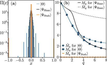
Figure 1: (a) Pauli spectrum for the atypical state $|\Theta\rangle$ (where we fix $\theta=2\arctan(\sqrt{2-\sqrt{3}})$ and $\phi=2\arctan(1-\sqrt{2})$), a typical (Haar random) state $|\Psi_{\mathrm{Haar}}\rangle$, and for a stabilizer state $|\Psi_{\mathrm{Stab}}\rangle$ generated by a random Clifford unitary for $N=10$ qubits. These distributions manifest distinctive traits, characterizing structural properties of magic. (b) The (filtered) stabilizer entropy ($\tilde{M}_{q}$) $M_{q}$ evaluated from the Pauli spectrum. Eq. (3) require exponential precision in $q$ to resolve between product and typical states, whereas for $\tilde{M}_{q}$ the separation is neat at any $q$. Both types of stabilizer entropy measure magic and lead to $M_{q}=\tilde{M}_{q}=0$ for stabilizer states.

Filtered stabilizer entropy. The distributions (4) and (5) imply that the SRE of a typical state is

$$M_{q}^{\mathrm{typ}}=\frac{1}{1-q}\log_{2}\left[\frac{(\eta-1)(2b)^{q}\Gamma\left(q+\frac{1}{2}\right)}{\sqrt{\pi}d}+\frac{1}{d}\right],$$ (6)

where $\Gamma(x)$ is the gamma function, $b$ is given above and ${\eta=d^{2}}$ (${\eta=D_{e}}$) for complex (real) typical states . Leveraging on the interpretation of SRE as the operator participation entropy, we anticipate the system size scaling of SRE as $M_{q}=D_{q}N+c_{q}$, with $D_{q}$ being the magic density and $c_{q}$ a sub-leading constant [37]. From (6), $D_{q}=1/(q-1)$ depends non-trivially on the index $q$ and vanishes in the large $q$ limit. (The subleading term in the ${N\to\infty}$ limit is ${c_{2}=-2}$ (${c_{2}=-\log_{2}\,7}$) and $c_{q>2}=0$ for generic (TRI) typical states.)

We contrast this behavior with the stabilizer entropy for the (atypical) product state $|\Theta\rangle=(\cos(\theta/2)|0\rangle+e^{-i\phi}\sin(\theta/2)|1\rangle)^{\otimes N}$ for generic $0<\theta<\pi/2$ and $\phi$. Although $M_{q}^{\Theta}\leq M_{q}^{\mathrm{typ}}$, we have the magic density $D_{q}^{\Theta}=1/(q-1)+\mathrm{O}(e^{-q})$ for large $q$, implying that the distinction between typical and atypical states is exponentially suppressed in the Rényi order $q$, cf.  Fig. 1. This counter-intuitive universality of magic density for $q\gg 1$ comes from the identity operator contribution, which, for typical states and large $N$, gives the leading contribution to $\zeta_{q}$ for any $q>2$.

Motivated by this, we introduce the filtered stabilizer entropy (FSE)

$$\tilde{M}_{q}\equiv\frac{1}{1-q}\log_{2}\left[\tilde{\zeta}_{q}\right],\quad\tilde{\zeta}_{q}\equiv\sum_{P\neq I}\frac{\langle\Psi|P|\Psi\rangle^{2q}}{d-1},$$ (7)

where the identity contribution is removed and $\tilde{\zeta}_{q}$ is normalized such that $\tilde{M}_{q}=0$ for the stabilizer states. While $\tilde{M}_{q}$ is functionally dependent on $M_{q}$, and hence is a magic measure [82], it readily distinguishes between typical and atypical quantum many-body states, cf. Fig 1. Thus, for typical states we find for the magic density $\tilde{M}_{q}=\tilde{D}_{q}N+\tilde{c}_{q}$ in the scaling limit, $\tilde{D}_{q}=1$ for all $q\geq 1$, while for the product state $\tilde{D}_{q}^{\Theta}=D_{q}^{\Theta}$. Furthermore, for typical complex (real) states we find $\tilde{c}_{q}=\log_{2}((2q-1)!!)/(1-q)$ [$\tilde{c}_{q}=\log_{2}((2q-1)!!)/(1-q)-1$], revealing a rich structure, absent for product states, which have $\tilde{c}_{q}=0$ for any $q$. In other words, $\tilde{M}_{q}$ reflects the structural properties of typical states at a polynomially subleading order in system size, similarly to the participation entropy quantifying state spread in the computational basis [83, 84, 54].

Pauli spectrum of Haar random states. As our next step, we justify the assumptions behind (4) and (5) for Haar-random states by explicitly evaluating their Pauli spectrum and SRE.

We first consider the Haar-random real states, described by the circular orthogonal ensemble (COE) [85, 86]. The general complex case corresponds to the circular unitary ensemble (CUE) and uses similar arguments, as detailed below. The COE states are given by $|\Psi\rangle=O|0\rangle^{\otimes N}$, where $O\in\mathcal{O}(d)$ is a real orthogonal matrix. Due to reality of $|\Psi\rangle$, only the $D_{e}$ real Pauli strings $P=P^{T}$ may have $x=\langle\Psi|P|\Psi\rangle\neq 0$. An appropriate orthogonal transformation can bring them to diagonal form $P^{D}$. Because of Haar invariance, the distributions of $x$ and $\tilde{x}=\langle\Psi|P^{D}|\Psi\rangle$ are the same. In all cases, except for $P=I$, $P^{D}$ has equal number of $d/2$ eigenvalues $\pm 1$. We denote $\mathbb{P}_{\pm}$ the projections on the respective (degenerate) eigenspaces. Then, the Haar distributed state is described by the polyspherical coordinates [87] $|\Psi\rangle=\cos(\theta)\mathbb{P}_{+}|\Psi\rangle+\sin(\theta)\mathbb{P}_{-}|\Psi\rangle$, and $\tilde{x}=\cos(2\theta)$. In this coordinate system, the induced measure is [88],

$$\Pi_{d}(\theta)=\frac{2\left(\sin(\theta)\cos(\theta)\right)^{d/2-1}}{B(d/4,d/4)},$$ (8)

with $B(x,y)$ being the Beta function. Transforming back the distribution (with the additional Jacobian factor) and keeping into account the separate contribution for $P=I$ and $D_{o}$ Pauli strings with $P^{T}=-P$, we find

$$\begin{split}\Pi_{d}^{\mathrm{COE}}(x)&=\frac{1}{d^{2}}\delta(x-1)+\frac{D_{o}}{d^{2}}\delta(x)\\ &\ +\frac{D_{e}-1}{d^{2}}\frac{\left(1-x^{2}\right)^{d/4-1}\Gamma\left(\frac{1}{4}\left(2+d\right)\right)}{\sqrt{\pi}\Gamma\left(d/4\right)}.\end{split}$$ (9)

A similar argument applies for $|\Psi\rangle=U|0\rangle^{\otimes N}$ with a Haar-random unitary $U\in\mathcal{U}(d)$. The differences are: (i) any $P\neq I$ is unitary diagonalizable into the same $P^{D}$, (ii) the random state $|\Psi\rangle$ is complex. As before we introduce $\tilde{x}=\langle\Psi|P^{D}|\Psi\rangle$. Viewing the $d$-dimensional Hilbert space as $\mathbb{R}^{2d}$, we divide the state into real and imaginary parts and similarly factorize the operator $P^{D}$. It follows then the resulting distribution is simply given by $\Pi_{d}(\theta)=2(\sin(\theta)\cos(\theta))^{d-1}/B(d/2,d/2)$. Transforming back with $\theta=\arccos(x)/2$ and the $P=I$ term yields

$$\begin{split}\Pi_{d}^{\mathrm{CUE}}(x)&=\frac{1}{d^{2}}\delta(x-1)+\frac{d^{2}-1}{d^{2}}\frac{\left(1-x^{2}\right)^{d/2-1}\Gamma\left(\frac{d+1}{2}\right)}{\sqrt{\pi}\Gamma\left(d/2\right)}.\end{split}$$ (10)

An alternative derivation of (10) making a connection with $k$-design is delegated to [82]. We note that, in the limit ${N\to\infty}$, (9) and (10) converge to typicality-based distributions (5) and (4), validating our assumptions above. As a consequence, the values of $M_{q}$ and $\tilde{M}_{q}$ discussed above accurately capture $q$-dependence of SRE and FSE for Haar random states, for any $N$, see [82].

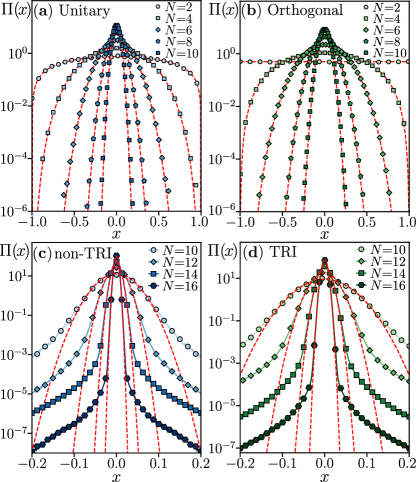
Figure 2: Pauli spectra of typical states (red dashed lines, Eq. (4) and  (5)) and the numerical results for: random unitary circuits (a), random orthogonal circuits (b), mid-spectrum eigenstates of chaotic Hamiltonian $H^{\mathrm{sb}}$ without TRI, (c), and with TRI $H$, (d), see Text. Only the regular parts of the distributions are plotted.

Pauli Spectra and filtered stabilizer entropy of chaotic systems. We numerically investigate PS and the FSE in quantum many-body systems to demonstrate the physical relevance of the typicality picture. Since the Pauli spectrum contains $4^{N}$ elements, its direct evaluation is only possible for systems comprising a small ${N\lesssim 12}$ number of qubits. To extend the range of accessible system sizes, we employ the following sampling procedure. To probe state $\ket{\Psi}$, we associate each Pauli string $P$$\neq$$I$ with a probability $\rho(P)$$=$$\langle\Psi|P|\Psi\rangle^{2}/(d-1)$, and put $\rho(I)$$=$$0$ . We sample the resulting probability distribution over the Pauli strings using the Metropolis-Hastings algorithm [90, 91]. Initialized in a random Pauli string $P_{1}$, such that $\rho(P_{1})>\epsilon$ (we select $\epsilon=10^{-14}$), the algorithm performs $\mathcal{N}-1\gg 1$ steps and outputs a sequence of Pauli strings $P_{1},\ldots,P_{\mathcal{N}}$. At the $k$-th step, the algorithm generates a candidate Pauli string $P^{\prime}_{k+1}$ by multiplying $P_{k}$ by two operators selected with uniform probability from the set $\{X_{1},Z_{1},\ldots,X_{N},Z_{N}\}$. The candidate Pauli string is accepted ($P_{k+1}$$=$$P^{\prime}_{k+1}$) with probability $p_{\mathrm{acc}}=\min\{1,\rho(P^{\prime}_{k+1})/\rho(P_{k+1})\}$, or, otherwise, it is rejected ($P_{k+1}$$=$$P_{k}$). On average, the algorithm outputs $\mathcal{N}\rho(P)$ Pauli strings $P$. This allows us to approximate the Pauli spectrum as $\Pi(x)=\sum_{k=1}^{\mathcal{N}}\rho(P_{k})^{-1}\delta(x-\bra{\Psi}P\ket{\Psi})$, and calculate the FSE (7) as $\tilde{M}_{q}=\log_{2}((d-1)^{q-1}\sum_{k=1}^{\mathcal{N}}\rho(P_{k})^{q-1})/(1-q)$. Eliminating the identity Pauli string $I$ (which otherwise would have an anomalously large weight) makes this sampling procedure efficient for typical quantum states that we consider here. In contrast, for a stabilizer state, the $p_{\mathrm{acc}}$ is exponentially small in $N$, and the algorithm less efficient than the approaches of [40, 39, 38]. Here, we reach system sizes up to $N=20$ by setting $\mathcal{N}=10^{6}$ for $N\leq 16$ and $\mathcal{N}=10^{5}$ for $16<N\leq 20$.

As a first numerical example, we consider brick-wall quantum circuits [18] with local two-qubit gates drawn from the Haar distribution on the unitary and orthogonal group, cf. [82] for details. Our results, for circuits of depth $T\sim\mathcal{O}(N)$, demonstrate that the Pauli spectra $\Pi(x)$ in (9) and (10) are reproduced, see Fig. 2(a,b). This fact is expected since random circuits approximate the full Haar distribution being approximate $k$-designs [68, 92].

Now, we turn to eigenstates of ergodic quantum systems [93, 94], and focus on the Ising model

$$H=\sum_{i=1}^{N}gX_{i}+\sum_{i=1}^{N}h_{i}Z_{i}+\sum_{i=1}^{N-1}JZ_{i}Z_{i+1}.$$ (11)

We set open boundary conditions and follow the parameter choice of [95]: $J$$=$$1$, $g$$=$$(\sqrt{5}+5)/8$, $h_{i}$$=$$(\sqrt{5}+1)/4$ for $i=2,\ldots,N$ and $h_{1}$$=$$-J$. With those specifications, (11) is quantum ergodic, with level statistics following the COE universality. We also consider breaking the TRI by $H_{1}=Y_{L-2}Z_{L-1}+Y_{L-1}Z_{L}$, resulting in the model $H^{\mathrm{sb}}=H+H_{1}$ with level statistics conforming to CUE universality. We calculate $n_{\mathrm{ev}}=\min\{d/10,10^{4}\}$ mid-spectrum eigenstates of $H$ and $H^{\mathrm{sb}}$ with POLFED algorithm [96, 97] for $10\leq N\leq 20$, perform the sampling of Pauli strings with the Metropolis-Hastings algorithm, and average the results over the eigenstates.

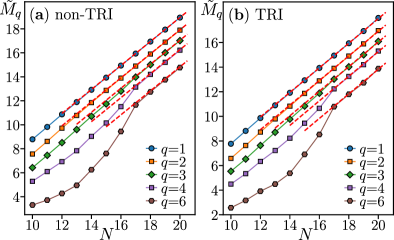
Figure 3: The filtered stabilizer entropy $\tilde{M}_{q}$ at $q=1,\dots,6$ for the random Haar states (red dashed lines) and eigenstates of chaotic Hamiltonian for systems (markers) without (a) and with (b) time-reversal invariance. The data for distinct $q$ are shifted downwards by $(q-1)/2$ for clarity.

We obtain quantitatively similar Pauli spectra $\Pi(x)$ for both $H$ and $H^{\mathrm{sb}}$, as shown in Fig. 2. The spectra follow the Haar state predictions (10) and (9), respectively, for the systems without and with TRI, down to a tail, which decays exponentially with $x$, and with the weight being exponentially suppressed in $N$. The Gaussian core of $\Pi(x)$ around zero indicates that the expectation value of Pauli strings in chaotic eigenstates tends to be exponentially close to zero as a function of $N$. This trend is prevalent among the vast majority of Pauli strings, which are typically non-local operators, and hence, their description is beyond the standard formulation of ETH, cf. [98, 99, 100]. The tails of $\Pi(x)$ reflect a finer structure encoded in eigenstates of the Hamiltonian. Local Pauli strings, such as $P=X_{i}$, follow the ETH, exhibiting non-zero thermal expectation value $f_{P}(E)$ varying smoothly with energy $E$, up to fluctuations suppressed exponentially in $N$ [101, 102, 103, 104]. While instances of such local operators are exponentially rare in $\mathcal{P}_{N}$, they constitute one of the contributions to the tails of $\Pi(x)$; see [82] for further discussions. The presence of tails in $\Pi(x)$ is also visible in the behavior of the FSE shown in Fig. 3. With $q$ increasing, the tail affects the value of $\tilde{M}_{q}$ more, shifting it below the value of $\tilde{M}_{q}^{\mathrm{typ}}$ (6). However, due to the suppression of tails for large $N$, we again recover the typical scaling of FSE, $\tilde{M}_{q}=N+\tilde{c}_{q}$, for all considered values of $q$ for the mid-spectrum eigenstates of both $H$ and $H^{\mathrm{sb}}$.

Discussion and conclusion. We have demonstrated that the Pauli spectrum unveils the magic structural properties of many-qubit states. We proposed a phenomenological picture of the Pauli spectrum based on quantum typicality, which we corroborated by deriving the exact expressions for random Haar states. Observing that the identity operator contribution dominates the value of stabilizer entropies for Rényi index $q>2$, we have introduced the filtered stabilizer entropy (7). This measure of magic readily discriminates the typical states from the atypical ones, such as product states. Our extensive numerical simulations show that physically relevant states, such as those prepared by random circuits or mid-spectrum eigenstates of ergodic Hamiltonians, adhere to predictions of the typicality-based picture of the Pauli spectrum exponentially fast with the system size. Notably, the mid-spectrum eigenstates of chaotic Hamiltonians differ from the random circuit states and the Haar random states at the level of the Pauli spectrum by the presence of exponentially suppressed tails, which reveal richer structures encoded in the Hamiltonian.

We find that the filtered magic density is maximal, i.e., $\tilde{D}_{q}=1$, for typical states at any Renyi index $q$, demonstrating the challenges to prepare such states in digital quantum devices [105]. The Pauli spectrum encompasses the stabilizer entropies, enabling a more complete characterization of magic. Moreover, its adherence to results for typical states signals the ergodicity of the system. In general, it would be interesting to understand the structure of the Pauli spectrum when the ergodicity is broken, for instance, due to strong disorder or integrability, as well as its properties in the various phases of quantum matter.

Our results can be generalized to qudits, but for odd and prime local Hilbert space dimensions, the magic monotones [106, 107, 108, 109, 110] and their efficient sampling [111] have been demonstrated. Constructing magic monotones for qubits is still an outstanding problem. A high-end goal left for future work is building such magic monotones in terms of the Pauli spectrum – a task facilitated by the exact results presented here. Magic phase transitions, driven by competition of Clifford and non-Clifford resources [112, 113, 114, 115], constitute an interesting application of our results.

Supplemental Material:
Pauli Spectrum and Magic of Typical Quantum Many-Body States

The Supplemental Material contains

• An alternative proof of the main results and the explicit stabilizer entropy formulas for Haar random states;

• A description of properties of the filtered stabilizer entropy;

• Additional numerical results, including: the comparison between Haar random states and quantum circuits and discussion about the consistence of exponential tails of Pauli spectrum and eigenstate thermalization hypothesis.

1 Combinatoric derivation of typical stabilizer Rényi entropy and Pauli spectrum for Haar states.

In order to obtain the typical stabilizer Rényi entropy and the Pauli spectrum, we begin computing the Haar average $\overline{\zeta}_{q}\equiv\mathbb{E}_{U\sim\mathrm{Haar}}\zeta_{q}(U|0\rangle^{\otimes N})$, see also [116]. Recalling that $d=2^{N}$ is the Hilbert space dimension, the computation is recast in terms of $2q$ replicas

$$\overline{\zeta_{q}}=\mathbb{E}_{U\sim\mathrm{Haar}}\sum_{P\in\mathcal{P}_{N}}\frac{1}{d}\mathrm{Tr}\left(U^{\otimes(2q)}P^{\otimes(2q)}(U^{\dagger})^{\otimes(2q)}|\Psi\rangle\langle\Psi|^{\otimes(2q)}\right).$$ (S1)

Because of the linearity of the trace and the Haar average, we can exchange the order of the operations. The Haar average over the unitary group relies on the Schur-Weyl duality [69] and leads to

$$\overline{\zeta_{q}}=\sum_{\sigma\in S_{2q}}b_{\sigma}\mathrm{Tr}\left(T_{\sigma}|\Psi\rangle\langle\Psi|^{\otimes(2q)}\right)=\sum_{\sigma\in S_{2q}}b_{\sigma}$$ (S2)

where the coefficients $b_{\sigma}=\sum_{P\in\mathcal{P}_{N}}\sum_{\tau\in S_{2q}}W_{\sigma,\tau}\mathrm{Tr}(P^{(2q)}T_{\tau})/d$ have to be evaluated, and $W_{\sigma,\tau}$ is the Weingarten matrix [117, 116]. Since each Pauli string is given by $P=P_{1}\otimes P_{2}\otimes\cdots\otimes P_{N}$, with $P_{i}$ Pauli matrices acting on the $i$-th site, it follows that

$$b_{\sigma}=\sum_{\tau\in S_{2q}}W_{\sigma,\tau}\mathrm{Tr}\left(\Lambda_{q}^{\otimes N}T_{\tau}\right)$$ (S3)

where the $\Lambda_{q}=\sum_{P_{i}=I_{i},X_{i},Y_{i},Z_{i}}P^{\otimes(2q)}/2$ emerge from resummation of the local Pauli matrices. Furthermore, since $T_{\tau}=t_{\tau}^{\otimes N}$ acts independently on different sites [118], we have $b_{\sigma}=\sum_{\tau\in S_{2q}}W_{\sigma,\tau}\mathrm{Tr}(\Lambda_{q}t_{\tau})^{N}$. The form of $\Lambda_{q}$ implies that all permutations with the same cycle structure contribute equally. Furthermore, since $P_{i}^{2}=I_{i}$, $\delta_{P_{i},I_{i}}$ appears if any cycle has a odd number of elements. Collecting these facts, we have

$$\overline{\zeta_{q}}=\sum_{\sigma,\tau\in S_{2q}}W_{\sigma,\tau}\mathrm{Tr}(\Lambda_{q}t_{\tau})^{N}=\frac{1}{\prod_{i=0}^{q-1}(d+i)}\sum_{\lambda\vdash 2q}d_{\lambda}\begin{cases}2^{\mathrm{len}(\lambda)-1}&\text{if any cycle $r\in\lambda$ contains odd number of elements }\\ 2^{\mathrm{len}(\lambda)+1}&\text{otherwise.}\end{cases}$$ (S4)

In the above steps, $\lambda\vdash 2q$ are the cycle structures over $2q$ elements and $d_{\lambda}$ is the number of permutations whose cycle structure is the same of $\lambda$ [33], while $\mathrm{len}(\lambda)$ is the number of cycles in $\lambda$. The sum can be performed analytically, and gives

$$\overline{\zeta}_{q}=\frac{1}{d}\left(1+\frac{2\left(d-1\right)\Gamma\left(q+\frac{1}{2}\right)\Gamma\left(\frac{1}{2}\left(3+d\right)\right)}{\sqrt{\pi}\Gamma\left(\frac{2q+d+1}{2}\right)}\right).$$ (S5)

From (S5) we can already compute $M_{q}$ and $\tilde{M}_{q}$, which are self-averaging 

$$M_{q}^{\mathrm{typ}} =\frac{1}{1-q}\log_{2}\left[\frac{1}{d}\left(1+\frac{2\left(d-1\right)\Gamma\left(q+\frac{1}{2}\right)\Gamma\left(\frac{1}{2}\left(3+d\right)\right)}{\sqrt{\pi}\Gamma\left(\frac{2q+d+1}{2}\right)}\right)\right],$$ (S6)

$$\tilde{M}_{q}^{\mathrm{typ}} =\frac{1}{1-q}\log_{2}\left[\frac{2\Gamma\left(q+\frac{1}{2}\right)\Gamma\left(\frac{1}{2}\left(3+d\right)\right)}{\sqrt{\pi}\Gamma\left(\frac{2q+d+1}{2}\right)}\right].$$ (S7)

Next, we introduce the generating function [45]

$$f(z)=\sum_{q=1}^{N}\frac{1}{d}\overline{\zeta}_{q}z^{-q}=d\int dx\frac{x^{2}\Pi(x)}{z-x^{2}}$$ (S8)

where we used the definition of the Pauli spectrum $\Pi(x)$. Resumming the series, we find

$$f(z)=\frac{d^{-1}}{z-1}+\frac{(d-1)}{dz}{{}_{2}F_{1}\left(1,\frac{3}{2};\frac{1}{2}\left(3+d\right);\frac{1}{z}\right)}.$$ (S9)

Lastly $\Pi(x)$ is obtained via Cauchy integration (S8), leading to the Haar Pauli spectrum

$$\Pi_{d}^{\mathrm{CUE}}(x)=\frac{d^{2}-1}{d^{2}}\frac{\left(1-x^{2}\right)^{-1+d/2}\Gamma\left(\frac{1}{2}\left(1+d\right)\right)}{\sqrt{\pi}\Gamma\left(d/2\right)}+\frac{1}{d^{2}}\delta(x-1),$$ (S10)

recasting the result in the Main Text. In principle, similar considerations apply also in the time reversal invariant case (TRI). However, the Schur-Weyl duality for the orthogonal Haar group requires Brauer algebras, leading to more intricate computations [117, 120], which we do not pursue here. We instead report the typical $M_{q}$ and $\tilde{M}_{q}$, calculated from the exact form of the Pauli spectrum for the TRI case shown in the Main text, and given respectively by

$$M_{q}^{\mathrm{typ(TRI)}} =\frac{1}{1-q}\log_{2}\left[\frac{1}{d}\left(\frac{2(d-1)\Gamma\left(\frac{d+6}{4}\right)\Gamma\left(q+\frac{1}{2}\right)}{\sqrt{\pi}\Gamma\left(\frac{d+2}{4}+q\right)}+1\right)\right],$$ (S11)

$$\tilde{M}_{q}^{\mathrm{typ(TRI)}} =\frac{1}{1-q}\log_{2}\left[\frac{2\Gamma\left(\frac{d+6}{4}\right)\Gamma\left(q+\frac{1}{2}\right)}{\sqrt{\pi}\Gamma\left(\frac{d+2}{4}+q\right)}\right].$$ (S12)

In the scaling limit, these results converge to the phenomenological values of SRE and FSE discussed in the Main Text.

2 Properties of the filtered stabilizer entropy

From its definition, it is clear that the filtered stabilizer entropy is related to the stabilizer entropy. Indeed, we have, cf. Main Text,

$$\tilde{\zeta}_{q}=\frac{d\zeta_{q}-1}{d-1}.$$ (S13)

It follows that (I) $\tilde{\zeta}_{q}(|\Psi\rangle)=1$ (hence $\tilde{M}_{q}=0$) for all $q$ iff $|\Psi\rangle$ is a stabilizer state, since $\zeta_{q}=1$ for all $q$ iff $|\Psi\rangle$ is a stabilizer state. Furthermore (II) $\tilde{\zeta}_{q}$ (hence $\tilde{M}_{q}$) is invariant under Clifford conjugation, namely $\tilde{\zeta}_{q}(C|\Psi\rangle)=\tilde{\zeta}_{q}(|\Psi\rangle)$ for any Clifford unitary $C\in\mathcal{C}_{N}$. This follows from the definition of $\tilde{\zeta}_{q}$ and the fact that Pauli strings are mapped to single Pauli strings by Clifford unitaries. Lastly, (III) $\tilde{M}_{q}$ is subadditive. Consider a product state $|\Psi\rangle=|\psi_{A}\rangle\otimes|\psi_{B}\rangle$, with $|\psi_{A}\rangle$ leaving in the $d_{A}=2^{N_{A}}$ dimensional Hilbert space of $N_{A}$ qubits, and $|\psi_{B}\rangle$ on the $d_{B}=d/d_{A}=2^{N_{B}}$ complementary space on $N_{B}=N-N_{A}$ qubits. It follows that

$$\begin{split}\tilde{\zeta}_{q}(|\Psi\rangle)&=\sum_{P\neq I,P\in\mathcal{P}_{N}}\frac{\langle\Psi|P|\Psi\rangle^{2q}}{d-1}=\frac{(d_{A}-1)d_{B}}{d-1}\left(\sum_{P_{A}\neq I,P_{A}\in\mathcal{P}_{N_{A}}}\frac{\langle\psi_{A}|P_{A}|\psi_{A}\rangle^{2q}}{d_{A}-1}\right)\left(\sum_{P_{B}\in\mathcal{P}_{N_{B}}}\frac{\langle\psi_{B}|P_{B}|\psi_{B}\rangle^{2q}}{d_{B}}\right)\\ &=\frac{(d_{A}-1)d_{B}}{d-1}\tilde{\zeta}_{q}(|\psi_{A}\rangle)\zeta_{q}(|\psi_{B}\rangle=\frac{(d_{A}-1)}{d-1}\tilde{\zeta}_{q}(|\psi_{A}\rangle)[(d_{B}-1)\tilde{\zeta}_{q}(|\psi_{B}\rangle)+1]\geq\tilde{\zeta}_{q}(|\psi_{A}\rangle)\tilde{\zeta}_{q}(|\psi_{B}\rangle)\end{split}$$ (S14)

and in particular $\tilde{M}_{q}(|\Psi\rangle)\leq\tilde{M}_{q}(|\psi_{A}\rangle)+\tilde{M}_{q}(|\psi_{B}\rangle)$. Furthermore, in the scaling limit $N_{A},N_{B}\to\infty$, the inequality is saturated. Hence, (IIIbis) $\tilde{M}_{q}$ is asymptotically additive. Nevertheless, $\tilde{M}_{q}$ is non-monotone. The proof follows from the explicit counterexamples in [38], which show that the FSE $\tilde{M}_{q}$ fails to be monote in the same way as the SRE $M_{q}$.

3 Additional numerical results

For completeness, we include a numerical test of random circuits generated by CUE and COE two-body gates. The architecture is the brickwall circuit, with each unitary layer given by

$$U_{t}=\prod_{i=1}^{N/2}\begin{cases}U_{2i-1,2i}&\text{if }t\text{ is even},\\ U_{2i,2i+1}&\text{otherwise},\end{cases}$$ (S15)

and periodic boundary conditions are assumed. The unitaries $U_{i,j}$ are drawn from $\mathcal{U}(4)$ ($\mathcal{O}(4)$) for CUE (COE) circuits. We evolve the state $|\Psi_{t_{\mathrm{max}}}\rangle=U^{t}|0\rangle^{\otimes N}$ up to $t_{\mathrm{max}}=L$ depth, and compute the average stabilizer entropy with $\mathcal{N}_{\mathrm{real}}=1000$ disorder realizations. The results are summarized in Fig. S1. We find that, up to the statistical errors associated with the number of circuit realizations and sampling of FSE with the Monte Carlo method (at $N>12$), the exact Haar predictions match the finite depth circuit numerics, providing a strong benchmark of our analytical arguments. In the same fashion, the average $\tilde{M}_{q}$ match the exact formulae (S12) and (S7) for TRI (Fig. S1(b) ) and non-TRI (Fig. S1(d)) systems, respectively.

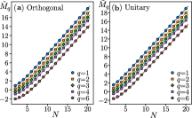
Figure S1: Exact formulas for the FSE of Haar random states (solid lines) vs numerical data (points) for COE (a) and CUE (b). The FSE are shifted by $(q-1)/2$ for clarity of the plots.

Finally, we identify one of the contributions to the tails of the Puali spectra of chaotic eigenstates. The ETH ansatz, typically formulated for a local observable $O$ and an eigenstate $\ket{\Psi}$ of an ergodic Hamiltonian $H$, (with $H\ket{\Psi}=E\ket{\Psi}$) implies that

$$\bra{\Psi}O\ket{\Psi}=f_{O}(E)+\Sigma_{O}(E),$$ (S16)

where $f_{O}(E)$ is a smooth function of energy $E$, and $\Sigma_{O}(E)$ represents fluctuations that are suppressed exponentially with $N$. In the following, we discuss how (S16) is reflected in the Pauli spectra $\Pi(x)$ of the chaotic eigenstates.

The Pauli spectra shown in the Fig. 2 of the Main Text consist of a well-pronounced Gaussian core and the exponentially suppressed tail. This implies that the fraction of the Pauli strings $P$ that satisfy equation (S16) with $f_{P}(E)=0$, at the probed energies $E$ close to the middle of the spectrum of the considered Ising models, is increasing, towards unity, with $N$. Moreover, the fluctuations $\Sigma_{O}(E)$ for such operators are decaying exponentially with $N$. Notably, these Pauli strings are typically highly non-local operators.

The local structure of the mid-spectrum eigenstates of Ising model is reflected in properties of Pauli strings $P_{\mathrm{loc}}$ that are local operators. Since the Ising model is ergodic, the ETH ansatz (S16) applies with $O=P_{\mathrm{loc}}$. Importantly, for certain types of local Pauli string, we find that $f_{P_{\mathrm{loc}}}(E)\neq 0$, and that $f_{P_{\mathrm{loc}}}(E)$ does not converge to $0$ with increasing $N$. The ratio of the number of the local Pauli strings to the total number of Pauli strings included in $\mathcal{P}_{N}$ is, however, exponentially small in $N$. This results in one contribution to the exponential tails of the Pauli spectra observed in Fig. 2 of the Main Text. To provide concrete examples, we have considered $P_{\mathrm{loc}}$ to be $X_{i}$, $X_{i}X_{i+1}$, $Z_{i}$, or $Z_{i}Z_{i+1}$ and haven chosen $i$ away from the boundaries of the system. For operators $P_{\mathrm{loc}}=X_{i},Z_{i},Z_{i}Z_{i+1}$ we have found that $f_{P_{\mathrm{loc}}}(E)\neq 0$ (in passing, we note that each of those operators appears in the Hamiltonian of the Ising model). In contrast, certain local operators also exhibit $f_{P_{\mathrm{loc}}}(E)=0$, an example of such an operator is $X_{i}X_{i+1}$. The described properties are illustrated in Fig. S2.

The above considerations emphasize the role of the exponential tails as a feature the Pauli spectra that reflects the fine structure encoded in eigenstates of ergodic systems. While we have identified one mechanism which contributes to the exponential tails of the Pauli spectra, we have also verified that there exist rare non-local operators with atypically large expectations values which also contribute to the tails of the spectra. Understanding of the properties of such Pauli strings is left for future work. Notably, the exponential tails are absent in the Pauli spectra for the COE and CUE circuits implying total scrambling of the local quantum information at the considered circuit depths.

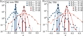
Figure S2: Local structure in the Pauli spectrum in mid-spectrum eigenstates of the Ising model. The Pauli strings $\sigma=X_{i}X_{i+1}$ (we consider $i=3,\ldots N-3$ to diminish the boundary effects) are distributed typically, according to a Gaussian distribution with standard deviation $\propto 2^{-L}$, decaying exponentially with the system size $L$, and with mean that converges rapidly to $0$. In contrast, the Pauli strings $P=X_{i}$ (for $i=3,\ldots N-3$) are distributed according to a Gaussian distribution with standard deviation $\propto 2^{-L}$, but with mean that converges to $x\neq 0$. The results are qualitatively the same for the model with TRI symmetry broken, as shown in panel (a), and in the TRI model, as shown in pabel (b).

References

- Bravyi and Kitaev [2005] S. Bravyi and A. Kitaev, Phys. Rev. A 71, 022316 (2005).
- Kitaev [2003] A. Kitaev, Ann. Phys. 303, 2 (2003).
- Gottesman and Chuang [1999] D. Gottesman and I. L. Chuang, Nature 402, 390 (1999).
- Veitch et al. [2014] V. Veitch, S. A. H. Mousavian, D. Gottesman, and J. Emerson, New J. Phys. 16, 013009 (2014).
- Bravyi et al. [2016] S. Bravyi, G. Smith, and J. A. Smolin, Phys. Rev. X 6, 021043 (2016).
- Chitambar and Gour [2019] E. Chitambar and G. Gour, Rev. Mod. Phys. 91, 025001 (2019).
- Liu and Winter [2022] Z.-W. Liu and A. Winter, PRX Quantum 3, 020333 (2022).
- Gottesman [1998] D. Gottesman, Phys. Rev. A 57, 127 (1998).
- Nielsen and Chuang [2000] M. A. Nielsen and I. L. Chuang, Quantum Computation and Quantum Information (Cambridge University Press, 2000).
- Eastin and Knill [2009] B. Eastin and E. Knill, Phys. Rev. Lett. 102, 110502 (2009).
- Nahum et al. [2017] A. Nahum, J. Ruhman, S. Vijay, and J. Haah, Phys. Rev. X 7, 031016 (2017).
- Zhou and Nahum [2019] T. Zhou and A. Nahum, Phys. Rev. B 99, 174205 (2019).
- Zhou and Nahum [2020] T. Zhou and A. Nahum, Phys. Rev. X 10, 031066 (2020).
- Sierant et al. [2023a] P. Sierant, M. Schirò, M. Lewenstein, and X. Turkeshi, Phys. Rev. Lett. 131, 230403 (2023a).
- Fritzsch and Prosen [2021] F. Fritzsch and T. Prosen, Phys. Rev. E 103, 062133 (2021).
- Claeys and Lamacraft [2021] P. W. Claeys and A. Lamacraft, Phys. Rev. Lett. 126, 100603 (2021).
- Li et al. [2019] Y. Li, X. Chen, and M. P. A. Fisher, Phys. Rev. B 100, 134306 (2019).
- Fisher et al. [2023] M. P. Fisher, V. Khemani, A. Nahum, and S. Vijay, Annu. Rev. Condens. Matter Phys. 14, 335 (2023).
- Potter and Vasseur [2022] A. C. Potter and R. Vasseur, Quantum Sciences and Technology (Springer, Cham, 2022) p. 211.
- Sierant et al. [2022] P. Sierant, M. Schirò, M. Lewenstein, and X. Turkeshi, Phys. Rev. B 106, 214316 (2022).
- Jian et al. [2020] C.-M. Jian, Y.-Z. You, R. Vasseur, and A. W. W. Ludwig, Phys. Rev. B 101, 104302 (2020).
- Li et al. [2021] Y. Li, R. Vasseur, M. P. A. Fisher, and A. W. W. Ludwig, (2021), arXiv:2110.02988 [cond-mat.stat-mech] .
- Gottesman [1997] D. Gottesman, arXiv:9705052 (1997).
- Aaronson and Gottesman [2004] S. Aaronson and D. Gottesman, Phys. Rev. A 70, 052328 (2004).
- Beverland et al. [2020] M. Beverland, E. Campbell, M. Howard, and V. Kliuchnikov, Quantum Sci. Technol. 5, 035009 (2020).
- Note [1] Compared to [25], we prefer to avoid the absolute value in the definition, allowing for a more precise characterization. Reverting to [25] from (1) is straightforward.
- Jiang and Wang [2023] J. Jiang and X. Wang, Phys. Rev. Appl. 19, 034052 (2023).
- Leone et al. [2023a] L. Leone, S. F. E. Oliviero, and A. Hamma, (2023a), arXiv:2305.15398 [quant-ph] .
- Qassim et al. [2021] H. Qassim, H. Pashayan, and D. Gosset, Quantum 5, 606 (2021).
- Leone et al. [2022] L. Leone, S. F. E. Oliviero, and A. Hamma, Phys. Rev. Lett. 128, 050402 (2022).
- Haug et al. [2023] T. Haug, S. Lee, and M. S. Kim, (2023), arxiv:2305.19152 .
- Oliviero et al. [2022a] S. F. E. Oliviero, L. Leone, A. Hamma, and S. Lloyd, npj Quantum Inf. 8 (2022a).
- Turkeshi et al. [2023] X. Turkeshi, M. Schirò, and P. Sierant, Phys. Rev. A 108, 042408 (2023).
- Gu et al. [2023] A. Gu, L. Leone, S. Ghosh, J. Eisert, S. Yelin, and Y. Quek, A little magic means a lot (2023), arXiv:2308.16228 [quant-ph] .
- Tirrito et al. [2023] E. Tirrito, P. S. Tarabunga, G. Lami, T. Chanda, L. Leone, S. F. E. Oliviero, M. Dalmonte, M. Collura, and A. Hamma, (2023), arXiv:2304.01175 .
- Tarabunga and Castelnovo [2023] P. S. Tarabunga and C. Castelnovo, Magic in generalized rokhsar-kivelson wavefunctions (2023), arXiv:2311.08463 [quant-ph] .
- Haug and Piroli [2023a] T. Haug and L. Piroli, Phys. Rev. B 107, 035148 (2023a).
- Haug and Piroli [2023b] T. Haug and L. Piroli, Quantum 7, 1092 (2023b).
- Lami and Collura [2023] G. Lami and M. Collura, Phys. Rev. Lett. 131, 180401 (2023).
- Tarabunga et al. [2023] P. S. Tarabunga, E. Tirrito, T. Chanda, and M. Dalmonte, PRX Quantum 4, 040317 (2023).
- Chen et al. [2023] J. Chen, Y. Yan, and Y. Zhou, (2023), arXiv:2308.01886 [quant-ph] .
- Oliviero et al. [2021] S. F. Oliviero, L. Leone, and A. Hamma, Physics Letters A 418, 127721 (2021).
- Oliviero et al. [2022b] S. F. E. Oliviero, L. Leone, and A. Hamma, Phys. Rev. A 106, 042426 (2022b).
- Calabrese and Cardy [2004] P. Calabrese and J. Cardy, J. Stat. Mech. 2004, P06002 (2004).
- Calabrese and Lefevre [2008] P. Calabrese and A. Lefevre, Phys. Rev. A 78, 032329 (2008).
- Laflorencie [2016] N. Laflorencie, Phys. Rep. 646, 1 (2016).
- Goldstein et al. [2006] S. Goldstein, J. L. Lebowitz, R. Tumulka, and N. Zanghì, J. Stat. Phys. 125, 1193 (2006).
- Reimann [2007] P. Reimann, Phys. Rev. Lett. 99, 160404 (2007).
- Bartsch and Gemmer [2009] C. Bartsch and J. Gemmer, Phys. Rev. Lett. 102, 110403 (2009).
- Goold et al. [2016] J. Goold, M. Huber, A. Riera, L. del Rio, and P. Skrzypczyk, J. Phys. A: Math. Theor. 49, 143001 (2016).
- Note [2] Either a stabilizer state has elements +1, or it has elements +1 and elements -1.
- Luitz et al. [2014a] D. J. Luitz, F. Alet, and N. Laflorencie, Phys. Rev. B 89, 165106 (2014a).
- Luitz et al. [2014b] D. J. Luitz, F. Alet, and N. Laflorencie, Phys. Rev. Lett. 112, 057203 (2014b).
- Sierant and Turkeshi [2022] P. Sierant and X. Turkeshi, Phys. Rev. Lett. 128, 130605 (2022).
- Deutsch [1991] J. M. Deutsch, Phys. Rev. A 43, 2046 (1991).
- Srednicki [1994] M. Srednicki, Phys. Rev. E 50, 888 (1994).
- Rigol et al. [2008] M. Rigol, V. Dunjko, and M. Olshanii, Nature 452, 854 (2008).
- Foini and Kurchan [2019a] L. Foini and J. Kurchan, Phys. Rev. Lett. 123, 260601 (2019a).
- Foini and Kurchan [2019b] L. Foini and J. Kurchan, Phys. Rev. E 99, 042139 (2019b).
- Dymarsky and Liu [2019] A. Dymarsky and H. Liu, Phys. Rev. E 99, 010102 (2019).
- Brenes et al. [2020a] M. Brenes, S. Pappalardi, J. Goold, and A. Silva, Phys. Rev. Lett. 124, 040605 (2020a).
- Pappalardi et al. [2022] S. Pappalardi, L. Foini, and J. Kurchan, Phys. Rev. Lett. 129, 170603 (2022).
- Pappalardi et al. [2023a] S. Pappalardi, F. Fritzsch, and T. Prosen, (2023a), arXiv:2303.00713 [cond-mat.stat-mech] .
- Pappalardi et al. [2023b] S. Pappalardi, L. Foini, and J. Kurchan, (2023b), arXiv:2304.10948 [cond-mat.stat-mech] .
- Wang et al. [2022] J. Wang, M. H. Lamann, J. Richter, R. Steinigeweg, A. Dymarsky, and J. Gemmer, Phys. Rev. Lett. 128, 180601 (2022).
- Dymarsky [2022] A. Dymarsky, Phys. Rev. Lett. 128, 190601 (2022).
- Wang et al. [2023] J. Wang, J. Richter, M. H. Lamann, R. Steinigeweg, J. Gemmer, and A. Dymarsky, (2023), arXiv:2310.20264 [cond-mat.stat-mech] .
- Brandão et al. [2016] F. G. S. L. Brandão, A. W. Harrow, and M. Horodecki, Comm. Math. Phys. 346, 397 (2016).
- Roberts and Yoshida [2017] D. A. Roberts and B. Yoshida, J. High Energy Phys. 2017 (4).
- Ippoliti and Ho [2022] M. Ippoliti and W. W. Ho, Quantum 6, 886 (2022).
- Cotler et al. [2023] J. S. Cotler, D. K. Mark, H.-Y. Huang, F. Hernández, J. Choi, A. L. Shaw, M. Endres, and S. Choi, PRX Quantum 4, 010311 (2023).
- Ippoliti and Ho [2023] M. Ippoliti and W. W. Ho, PRX Quantum 4, 030322 (2023).
- Fava et al. [2023] M. Fava, J. Kurchan, and S. Pappalardi, (2023), arXiv:2308.06200 [quant-ph] .
- Luitz and Bar Lev [2016] D. J. Luitz and Y. Bar Lev, Phys. Rev. Lett. 117, 170404 (2016).
- Luitz [2016] D. J. Luitz, Phys. Rev. B 93, 134201 (2016).
- Brenes et al. [2020b] M. Brenes, J. Goold, and M. Rigol, Phys. Rev. B 102, 075127 (2020b).
- Mondaini and Rigol [2017] R. Mondaini and M. Rigol, Phys. Rev. E 96, 012157 (2017).
- Richter et al. [2020] J. Richter, A. Dymarsky, R. Steinigeweg, and J. Gemmer, Phys. Rev. E 102, 042127 (2020).
- Brenes et al. [2021] M. Brenes, S. Pappalardi, M. T. Mitchison, J. Goold, and A. Silva, Phys. Rev. E 104, 034120 (2021).
- Brenes et al. [2020c] M. Brenes, T. LeBlond, J. Goold, and M. Rigol, Phys. Rev. Lett. 125, 070605 (2020c).
- Note [3] We note that, since is exponentially narrow in system size for typical states, the stabilizer entropy is self-averaging.
- sup [2023] See the supplementary material. (2023).
- Macé et al. [2019] N. Macé, F. Alet, and N. Laflorencie, Phys. Rev. Lett. 123, 180601 (2019).
- Bäcker et al. [2019] A. Bäcker, M. Haque, and I. M. Khaymovich, Phys. Rev. E 100, 032117 (2019).
- Mehta [2004] M. L. Mehta, Random Matrices, 3rd ed. (Academic Press, New York, 2004).
- Haake [2010] F. Haake, Quantum Signatures of Chaos (Springer, Berlin, 2010).
- Chapuisat and Iung [1992] X. Chapuisat and C. Iung, Phys. Rev. A 45, 6217 (1992).
- Klimyk and Vilenkin [1995] A. Klimyk and N. Y. Vilenkin, in Representation Theory and Noncommutative Harmonic Analysis II: Homogeneous Spaces, Representations and Special Functions (Springer, 1995) pp. 137–259.
- Note [4] The identity implies that .
- Metropolis et al. [1953] N. Metropolis, A. W. Rosenbluth, M. N. Rosenbluth, A. H. Teller, and E. Teller, J. Chem. Phys. 21, 1087 (1953).
- Hastings [1970] W. K. Hastings, Biometrika 57, 97 (1970).
- Haferkamp [2022] J. Haferkamp, Quantum 6, 795 (2022).
- Luca D’Alessio and Rigol [2016] A. P. Luca D’Alessio, Yariv Kafri and M. Rigol, Adv. Phys. 65, 239 (2016).
- Abanin et al. [2019] D. A. Abanin, E. Altman, I. Bloch, and M. Serbyn, Rev. Mod. Phys. 91, 021001 (2019).
- Kim and Huse [2013] H. Kim and D. A. Huse, Phys. Rev. Lett. 111, 127205 (2013).
- Sierant et al. [2020] P. Sierant, M. Lewenstein, and J. Zakrzewski, Phys. Rev. Lett. 125, 156601 (2020).
- Sierant et al. [2023b] P. Sierant, M. Lewenstein, A. Scardicchio, and J. Zakrzewski, Phys. Rev. B 107, 115132 (2023b).
- Khaymovich et al. [2019] I. M. Khaymovich, M. Haque, and P. A. McClarty, Phys. Rev. Lett. 122, 070601 (2019).
- Łydżba et al. [2021] P. Łydżba, Y. Zhang, M. Rigol, and L. Vidmar, Phys. Rev. B 104, 214203 (2021).
- Ulčakar and Vidmar [2022] I. Ulčakar and L. Vidmar, Phys. Rev. E 106, 034118 (2022).
- Beugeling et al. [2014] W. Beugeling, R. Moessner, and M. Haque, Phys. Rev. E 89, 042112 (2014).
- Ikeda et al. [2013] T. N. Ikeda, Y. Watanabe, and M. Ueda, Phys. Rev. E 87, 012125 (2013).
- Dymarsky et al. [2018] A. Dymarsky, N. Lashkari, and H. Liu, Phys. Rev. E 97, 012140 (2018).
- Mierzejewski and Vidmar [2020] M. Mierzejewski and L. Vidmar, Phys. Rev. Lett. 124, 040603 (2020).
- Preskill [2018] J. Preskill, Quantum 2, 79 (2018).
- Gross [2006a] D. Gross, J. Math. Phys. 47, 122107 (2006a).
- Gross [2006b] D. Gross, Appl. Phys. B 86, 367–370 (2006b).
- Howard and Campbell [2017] M. Howard and E. Campbell, Phys. Rev. Lett. 118, 090501 (2017).
- White et al. [2021] C. D. White, C. Cao, and B. Swingle, Phys. Rev. B 103, 075145 (2021).
- White and Wilson [2020] C. D. White and J. H. Wilson, (2020), arXiv:2011.13937 .
- Tarabunga [2023] P. S. Tarabunga, (2023), arXiv:2309.00676 [quant-ph] .
- Leone et al. [2023b] L. Leone, S. F. E. Oliviero, G. Esposito, and A. Hamma, (2023b), arXiv:2302.07895 .
- Niroula et al. [2023] P. Niroula, C. D. White, Q. Wang, S. Johri, D. Zhu, C. Monroe, C. Noel, and M. J. Gullans, (2023), arXiv:2304.10481 [quant-ph] .
- Bejan et al. [2023] M. Bejan, C. McLauchlan, and B. Béri, (2023), arXiv:2312.00132 [quant-ph] .
- Fux et al. [2023] G. E. Fux, E. Tirrito, M. Dalmonte, and R. Fazio, (2023), arXiv:2312.02039 [quant-ph] .
- Turkeshi and Sierant [2023] X. Turkeshi and P. Sierant, (2023), arXiv:2308.06321 [quant-ph] .
- Collins and Śniady [2006] B. Collins and P. Śniady, Comm. Math. Phys. 264, 773 (2006).
- Gross et al. [2021] D. Gross, S. Nezami, and M. Walter, Commun. Math. Phys. 385, 1325 (2021).
- Note [5] Computing one finds .
- Molev and Rozhkovskaya [2012] A. I. Molev and N. Rozhkovskaya, J. Alg. Comb. 38, 15–35 (2012).