Nonequilibrium Dyson equations for strongly coupled light and matter:
spin glass formation in multi-mode cavity QED

Abstract

Light-matter interfaces have now entered a new stage marked by the ability to engineer quantum correlated states under driven-dissipative conditions. To propel this new generation of experiments, we are confronted with the need to model non-unitary many-body dynamics in strongly coupled regimes, by transcending traditional approaches in quantum optics. In this work, we contribute to this program by adapting a functional integral technique, conventionally employed in high-energy physics, in order to derive nonequilibrium Dyson equations for interacting light-matter systems. Our approach is grounded in constructing ’two-particle irreducible’ (2PI) effective actions, which provide a non-perturbative and conserving framework for describing quantum evolution at a polynomial cost in time. One of the aims of the article is to offer a pedagogical introduction designed to bridge readers from diverse scientific communities, including those in quantum optics, condensed matter, and high-energy physics. We apply our method to complement the analysis of spin glass formation in the context of frustrated multi-mode cavity quantum electrodynamics, initiated in our accompanying work [H. Hosseinabadi, D. Chang, J. Marino, arXiv:2311.05682]. Finally, we outline the capability of the technique to describe other near-term platforms in many-body quantum optics, and its potential to make predictions for this new class of experiments.

I Introduction

The field of quantum simulation has recently undergone a transformation, evolving into a new realm of research where the worlds of condensed matter physics and quantum optics merge. Today, an increasing array of platforms hosting many-body systems can accommodate both unitary and dissipative dynamics in a controlled fashion [1, 2, 3, 4, 5, 6]. This circumstance paves the way for the exploration of phases of matter and strongly correlated behavior that have no counterparts in either thermodynamic equilibrium or isolated non-equilibrium conditions.

In contrast to conventional solid-state systems, driven-dissipative condensed matter (a.k.a many-body quantum optics) systems exhibit a host of innovative characteristics. In the former, dissipation poses the primary challenge to quantum coherence, while in the latter, dissipation is at times intentionally harnessed or even engineered to drive the system into entangled states [7, 8, 9].

Traditional solid-state physics focuses on understanding equilibrium phases of matter that result from the interplay of interactions and thermal fluctuations [10, 11, 12, 13]. In the realm of driven-dissipative condensed matter, instead, emergent behavior can occur in dynamics or in the non-equilibrium steady state where the system settles. These novel responses usually arise from the intricate interplay of classical and quantum noise within the strongly coupled limit of a many-particle system. Finally, the nature of interactions fostering strong correlations takes on a fundamentally different character in the domain of quantum many-body optics. Here, short-range interactions originating from atoms or molecules coexist with long-range or even all-to-all interactions mediated by light, leading to fundamentally distinct cooperative mechanisms.

These distinctive features find natural occurrence in cavity quantum electrodynamics (cQED) experiments, which have occupied a central position in the field of driven-open quantum simulators for over a decade. In cavity QED, atoms and photons experience couplings as a consequence of their confinement within high-finesse optical cavities [14]. This confinement enables repeated light-matter scattering in nearly isolated conditions, achieving effectively strong interactions. The advent of ultra-cold quantum gases has made it possible to couple Bose-Einstein condensates to one or more photonic modes within such cavities, creating regimes of cooperative dynamics that intertwine matter waves and light [15]. Leveraging the flexibility, tunability, and engineering capabilities inherent in quantum simulators, these platforms have become ideal environments for realizing non-equilibrium phases of matter under driven-open conditions. These include phenomena such as dynamical ferromagnetism, super-solids, topological pumps, time crystals, spin networks, and many others [15]. Beyond fundamental research, applications extend to quantum information, where cavity QED currently holds the world record for spin squeezing [16, 17], an entangled state which surpasses classical limits for metrology and sensing.

In the majority of these experiments, the dynamical behavior of the system can be reduced to a few degrees of freedom: typically, these are photon amplitudes and numbers in conjunction with the dynamics of a collective spin that encapsulates the motion of the entire assembly of atoms [18, 19, 20, 21, 22, 23, 24, 25, 26, 27, 28, 29, 30, 31, 32, 33, 34]. This usually results from the all-to-all nature of photon-mediated interactions in the cavity, which allows for an effective mean-field description. Quantum fluctuations are sub-leading in the number of atoms when the dynamics of such macroscopic degrees of freedom are considered: only weak quantum noise influences the correlation between light and matter, and the system’s behavior can be effectively characterized through semi-classical descriptions [23].

This situation presents significant advantages when it comes to modeling cavity QED experiments, and it has certainly served as the foundation for constant advancements in joint theoretical and experimental efforts over the past fifteen years. Simultaneously, it naturally prompts the exploration of conditions where the strong correlations inherent in these systems become dominant. In this context, we are witnessing the emergence of a novel category of experiments, where the true many-body nature of the platform emerges and it defies a description using only a few macroscopic degrees of freedom. These experiments encompass a variety of setups, such as Rydberg tweezer arrays integrated into optical cavities [35], atomic ensembles with adjustable loading capacities [36, 37], and the fermionic variant of traditional cavity QED experiments [38].

All these experiments necessitate the integration of methods traditionally employed for addressing strongly correlated problems with the extra complication that detailed balance is broken and dynamics are non-unitary. Accessing the long-term evolution of open many-body systems subject to external (coherent or incoherent) drives as well as strong interactions, is one of the most challenging computational frontiers. Nevertheless, it has now become increasingly important in order to steer this new generation of cavity QED platforms.

Indeed, as numerous established platforms push the boundaries of the NISQ (Noisy Intermediate-Scale Quantum) era [39], a cavity QED platform endowed with strong correlations presents an intriguing opportunity. It would hold the potential for innovative strategies in quantum processing, leveraging the combined advantages offered by cooperative behavior [40], the interplay of long and short-range interactions [35, 41, 42], the manipulation of controllable quantum fluctuations [43], including the potential to manipulate decoherence channels [44].

As of today, state of art methods to model these experiments would encompass a number of options. Refined versions of semi-classical techniques, such as discrete phase space representations of the Hilbert space, have been tailored for addressing the driven-dissipative dynamics of spin and bosonic systems [45, 46, 47, 48, 49, 50]. Tensor network ansätze, which retain the most informaive correlations to describe dynamics, have been used to study phase transitions in driven open systems [51, 52, 53, 54, 55, 56, 57, 58]. At the same time, cluster mean field methods [59] or self-consistent Gaussian approximations [60] remain a straightforward, and, in some circumstances, competitive way, to qualitatively capture non-unitary dynamics.

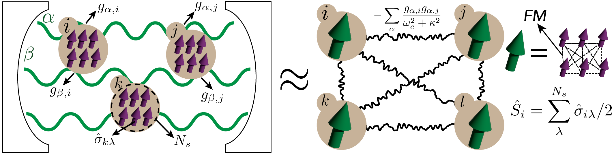
Figure 1: Schematics of the model considered in this work: $N$ clusters (tan circles) of $N_{s}$ two-level atoms (spins) interact with $M$ cavity modes (green lines) via static disordered couplings $g_{\alpha,i}$. Cavity modes mediate effective all-to-all interactions modulated among clusters. The effective interaction is modulated by static disorder and generates frustration and glassy dynamics. Each cluster can be taken as a large spin $S$ with amplitude $N_{s}/2$. Cavity modes induce ferromagnetic (FM) interactions between spins within the same cluster.

In this paper, we introduce a novel method to tackle the dynamics of strongly interacting light-matter systems in the many-body limit [61, 62]. It is an adaptation of the nonequilibrium Dyson equations (DE) derived from functional integrals in high energy physics and cosmology [63, 64, 65, 66, 67, 68, 69, 70, 71, 72, 73, 74, 75], and previously used also in the context of AMO and condensed matter [76, 77, 78, 79, 80, 81, 82, 83, 84]. Our method involves deriving an effective quantum action for the system as a function of its $n$-point correlation functions, from which DE descend following the least action principle [61, 62]. Here, we concentrate on deriving dynamics from what is referred to as the two-particle irreducible (2PI) effective action [63, 61, 62]. The term “two-particle irreducible” pertains to the Feynman diagrams contributing to the kernel of the DE, which cannot be separated into two parts by cutting at most two of their lines. Such action gives exact equations of motion of two-point functions, and with some ingenuity also the dynamics of higher point correlation functions [85, 86]. It is via a set of controlled non-perturbative approximations (large $N$ limit, dilute expansion, loop expansion) [61, 62, 79, 82] that the equations are actually solved numerically.

DE derived from 2PI effective actions offer numerous advantages. They descend from a variational principle, and therefore they give rise to self-consistent dynamics of two-point functions free from secular effects [62, 87]. Since approximations are directly performed at the level of the action, the resulting DE are conserving, in the sense they cannot spoil the conserved quantities of the original model. They also can seamlessly incorporate both coherent and dissipative dynamics, as functional integral methods do not markedly differentiate between the two [88]. They do not suffer from limitations when degrees of freedom with unbounded Hilbert space, like photons or phonons, are included in dynamics. The dynamics governed by DE have polynomial time costs in system size and they can be run on a personal computer. The price to pay is formulating educated guesses on the physics of the problem, which are crucial for selecting the proper approximation scheme. Furthermore, these DE are known to semi-quantitatively reproduce dynamics, and they are therefore excellent for elucidating the mechanisms at work in a given problem of interest, but less suited to fit with accuracy experimental curves, for instance. With these caveats, the method is highly flexible and applicable virtually to any driven-dissipative many particle system, made of fermions, bosons or spins, as we also expand in the conclusions of this manuscript.

In this work, we initiate our research program by applying this method to examine the dynamics of strongly correlated light-matter systems within multi-mode cavity QED. Our model is inspired by the experimental setup presented in Refs. [37, 89, 90, 91] which involves several photonic modes connecting nodes (Fig. 1). Each of these nodes houses atomic ensembles with adjustable loading capacities. By manipulating the number of atoms in each node (ranging from a few to thousands in the experiment) by using optical tweezers, one can introduce tunable quantum fluctuations in the platform. These fluctuations enable the exploration of system dynamics, from strongly correlated to semi-classical regimes. Importantly, this flexibility is not unique to this platform [36, 92] and represents a promising starting point for delving into many-body cavity QED beyond the domain of collective dynamic responses [19, 20]. During the final stages of the current work, the experiment detailed in Ref. [93] verified the existence of a spin glass (SG) phase within the quantum gas microscope platform of Refs. [37, 89, 90, 91] for the first time through direct measurement of the configuration of spins in the system. Notably, the observed spin-glass phase exhibits replica symmetry breaking [94], a distinctive and intriguing characteristic of certain models of SG, whose experimental verification is well-known to be a challenging task. In this paper, we complement the findings presented in our accompanying work on dynamical spin glass formation [95] by investigating the full spectrum of non-equilibrium phases and crossovers inherent to the experiment in [37, 89, 90, 91]. Furthermore, we offer a pedagogical introduction to the formalism of DE derived from effective actions. Our objective is to bridge the domains of AMO and the many-body community working at the interface of condensed matter and field theory.

I.1 Outline of the paper

The goal of this work is to understand the far from equilibrium dynamics of SG phases in frustrated cavity QED with strong disorder, where fluctuations cannot be omitted and mean field treatments are not applicable. We remark that our approach is distinct from those of Refs. [96, 97] which by construction, are suitable only for the universal SG behavior at steady state, in two key aspects. First, the formalism developed here is applicable in far from equilibrium situations such as quench dynamics, while keeping track of the quantum nature of spins. Second, the platform of Refs. [37, 89, 90, 91] naturally includes extra FM interactions which are unimportant in the steady state of the system [43], but as shown in this work, can qualitatively modify conventional SG dynamics away from equilibrium. We now briefly outline our key results which expand upon the results of our accompanying work [95].

Introduction to the model – We commence the paper by introducing the model in Section II. We will briefly review previous works on the behavior of the model in different regimes of parameters at the steady state, and will motivate using our approach to treat its far from equilibrium dynamics.

Introduction to the method – We provide a comprehensive introduction to effective action methods and non-equilibrium field theory in Section III. This introduction is anchored in a pedagogical example drawn from basic quantum mechanics – the dynamics of the anharmonic quantum oscillator. This serves as a foundation for the detailed derivation of our formalism in the context of frustrated light-matter interactions in cavity QED, covered in Section IV, where we develop a versatile approach to address real-time dynamics in a model for disordered cavity QED given in Fig. 1. To enhance accessibility, this section and its accompanying appendices are crafted to be reproducible from scratch by the interested reader. Readers with experience on 2PI methods can gloss over these two sections.

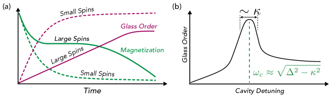
Figure 2: (a) Cartoon of the dependence of dynamics on spin size $N_{s}$ for initial states with finite magnetization. Small spins relax fast while for large spins, after an initial quick decay of FM order, the system enters a prethermal state with slowly decaying magnetization. SG order is built up faster for smaller spins. (b) Spin glass order versus cavity detuning $\omega_{c}$, showing a resonance close to atomic detuning $\Delta$.

Magnetization dynamics – In Section V.1, we show that the mean-field (MF) approximation, given by the leading order contribution in our approach, predicts a paramagnetic (PM) to ferromagnetic (FM) phase transition of effective spin degrees of freedom in the universality class of infinite range Ising model, but it completely omits the effect of frustrated interactions generated by static disorder in the system. FM interactions are mediated by virtual photon exchange processes among spins within the same cluster, and in contrast to inter-cluster couplings, are not frustrated. In Section V.2 we demonstrate that, upon the non-perturbative incorporation of disorder and fluctuations, our approach provides a dramatic improvement of MF results. As the focus of this work is the far from equilibrium dynamics of this system after interaction quenches, we first look at the dynamics of simple spin observables, such as global magnetization. We find that if the system is initiated in a symmetry broken state with a finite total magnetization, the relaxation of magnetic order substantially depends on the coupling strength and the size of atomic ensembles $N_{s}$ or equivalently, the amplitude of large spins $\hat{S_{i}}$ per each cluster (red curves in Fig. 2a). For weak couplings (Section V.2.1), global magnetization displays paramagnetic oscillations which are weakly damped due to the dephasing generated by static disorder. Upon increasing the coupling (Section V.2.2), spin relaxation changes from underdamped dynamics to overdamped dynamics without oscillations. In Section V.2.3 we address the effect of ensemble size $N_{s}$ on magnetization dynamics. We show that in the overdamped regime and for small $N_{s}$, global magnetization $\langle\hat{S}^{x}\rangle$ relaxes quickly to zero while for large $N_{s}$, it experiences an initial quick collapse to a finite value, and then stays in a transient prethermal state with a slow spiral decay of the magnetization vector along the axis of temporary FM order.

Dynamics of SG – To probe into the nature of the transition in the system as magnetization dynamics change from underdamped to overdamped, we consider more complex and richer spin observables in Section V.3. Particularly, and with the expectation of exploring SG order in the system, we consider the dynamics of two different order parameters for SG in Sections V.3.2 and V.3.3. First, we consider the disorder average of the square of local magnetization of each spin ensemble, a finite quantity in the glass phase, which measures how much the frozen spin state is protected from fluctuations. We extend the formalism of Keldysh field theory in order to access the real-time dynamics of this order parameter which is done for the first time in this work, although there is a technical similarity between our approach and the one introduced by Ref. [98] to study measurement-induced phase transitions. We confirm that the change in spin relaxation profile from underdamped to overdamped dynamics, indeed, happens when a PM to SG phase transition takes place in the system. In PM phase, the SG order parameter relaxes to zero after experiencing small temporary fluctuations. For quenches into SG phase, on the other hand, the order parameter relaxes to a finite value. Second, we consider the temporal correlations of spins over long times, conventionally known as the Edwards-Anderson (EA) [99, 100] order parameter, corresponding to the overlap of two snapshots of the system taken at long time intervals. We confirm that EA order parameter changes from zero in the PM phase, when the system loses its memory quickly, to a finite value in the SG phase, proving that the system is glassified. We proceed to show that spin fluctuations violate the fluctuation-dissipation theorem [101, 87], a phenomenon conjectured to be closely related to replica symmetry breaking in SG systems [102].

Effect of spin size – Section V.3.4 addresses the effect of ensemble size $N_{s}$ and initial conditions on the formation of SG phase. It is shown that the rate at which SG order builds up is slower for initial states with larger global magnetization, and is fastest if the system is initialized in the ground-state of non-interacting spins. The dependence on the initial state is found to be less significant for small $N_{s}$ and more pronounced for large ensemble sizes (green curves in Fig. 2a). The deceleration of SG formation for large clusters can be attributed to the long-lasting transient FM order mentioned above, which is protected by non-frustrated intra-cluster interactions, and acts as a competing order with SG [103, 104, 105, 106, 107] over intermediate timescales. For initial states with small net magnetization, the rate of SG formation is fastest and is not affected by cluster size. Notice that accessing the dynamics of atomic ensembles with tunable loading capacities is crucial for exploring the full spectrum of dynamical responses, not only in the experiment discussed in this work, but also in other cavity QED platforms [36]. This is in general a challenging task for conventional methods in quantum optics, while in our field theory approach this can be straightforwardly included since $N_{s}$ is natural parameter which appears naturally in our diagrammatic expansion.

Effect of resonant photons – In Section V.3.5, we consider the effect of photon frequency on the glass phase by looking at SG order parameter in a wide range of photon frequencies from fast photons to the resonance limit, where atomic and cavity detunings are close, and below. As shown schematically in Fig. 2b, SG order is peaked close to the resonance, while it saturates in the adiabatic limit. At frequencies below the resonance, SG order is dramatically suppressed, resembling the suppression of various types of order by low frequency lattice distortions (phonons) in solid state physics. We also address briefly the spectrum of low-lying excitations in the SG phase, showing a continuum of sub-Ohmic modes at small energies.

The capability to include in the same set of dynamical equations variable ranges of coupling, tunable values of $N_{s}$ and active photons, is one of the key merits of our approach. It allows us to solve for the dynamics of the full platform without the need to invoke large energy scale separations, effective descriptions suited only to atomic or photonic degrees of freedom, or to treat distinctly the quantum and semi-classical regimes. In this regard, the method has a degree of flexibility that appears promising to treat other strongly correlated driven-dissipative systems, as we discuss in the concluding Section VI.

II The Model

The experiment in [89, 37, 90, 91] can be modeled by a system of $N$ clusters, each one containing $N_{s}$ two-level atoms encoded by the spin-1/2 operators $\sigma_{i\lambda}$, with cluster $1\leq i\leq N$ and atom indices $1\leq\lambda\leq N_{s}$ , as shown in Fig. 1. The couplings between the atoms and the $M$ photonic modes of the cavity are spatial-dependent and uncorrelated from each other, which justifiemodellings their modeling via random spin-boson couplings [96, 97]. Starting from the same initial state for all spins, each cluster is equivalent to a single spin $S_{i}=\sum_{\lambda}\sigma_{i\lambda}/2$ with amplitude $S=N_{s}/2$. The parameter $S$ can be tuned by loading few or several atoms in each cluster, and it dictates the strength of quantum fluctuations. For instance, at large $S$ each cluster would be effectively described by a classical angular momentum, since its quantum noise would scale down as $1/S$ [19, 108, 109]. A minimal model for the system is given by the random Dicke model whose evolution is governed by $\partial_{t}\rho=-i\commutator{H}{\rho}+\sum_{\alpha=1}^{M}\mathcal{D}\quantity[a_{\alpha}]\rho$, where

$$H=\frac{\Delta}{2}\sum_{i,\lambda}\sigma^{z}_{i\lambda}+\sum_{\alpha}\omega_{\alpha}a^{\dagger}_{\alpha}a_{\alpha}\\ +\frac{1}{\sqrt{(M+N)N_{s}}}\sum_{\begin{subarray}{c}i,\lambda,\alpha\end{subarray}}g_{\alpha i}\quantity(a_{\alpha}+a_{\alpha}^{\dagger})\sigma^{x}_{i\lambda},$$ (1)

and

$$\mathcal{D}\quantity[a_{\alpha}]\rho=\kappa_{\alpha}\quantity(2a_{\alpha}\rho a_{\alpha}^{\dagger}-\anticommutator{a_{\alpha}^{\dagger}a_{\alpha}}{\rho}).$$ (2)

We assume that cavity modes are nearly degenerate such that $\omega_{\alpha}=\omega_{c}$ and $\kappa_{\alpha}=\kappa$. The couplings $g_{\alpha i}$ are assumed to be random and chosen from a Gaussian distribution:

$$\overline{g_{\alpha i}}=0,\quad\overline{g_{\alpha i}g_{\beta j}}=\delta_{\alpha\beta}\delta_{ij}g^{2}.$$ (3)

Couplings for spins in the same cluster are similar as we assume that the spatial size of each cluster is smaller than the wavelength of cavity modes. The scaling of the interaction term guarantees that the total energy is extensive in system size [110]. For $\omega_{c}\gg g,\Delta$ photons are the fastest degree of freedom in the problem; they quickly relax to stationary value and approximately, they mediate instantaneous interactions among spins. Assuming $\kappa=0$, photons can be adiabatically eliminated [111, 112, 113, 114, 43] and the model in (1) is mapped to

$$H_{\mathrm{eff}} =\sum_{i}H_{i}+H_{\mathrm{int}},$$ (4)

$$H_{i} \equiv\Delta S^{z}_{i}-\frac{4}{(N+M)N_{s}\omega_{c}}\quantity(\sum_{\alpha}g_{\alpha i}^{2})\quantity(S^{x}_{i})^{2},$$ (5)

$$H_{\mathrm{int}} \equiv-\frac{4}{(N+M)N_{s}\omega_{c}}\sum_{i\neq j}\sum_{\alpha}g_{\alpha i}g_{\alpha j}S^{x}_{i}S^{x}_{j},$$ (6)

where $S^{x}_{i}=\sum_{\lambda}\sigma^{x}_{i\lambda}/2$ is the total spin operator for each cluster. For $N_{s}>1$, each cluster in Eq. (5) is an infinite range quantum Ising model also known as the Lipkin-Meshkov-Glick [115] (LMG) model with Hamiltonian

$$H_{\mathrm{LMG}}=\Delta S^{z}-\frac{J}{N_{s}}(S^{x})^{2}.$$ (7)

$H_{\mathrm{LMG}}$ admits an exact solution using mean-field theory in the limit $N_{s}\to\infty$, and features a paramagnet (PM) to FM phase transition [116, 117, 118, 24, 119, 120] at $\Delta=J$. The effective interactions between atoms within the same cluster in Eq. (5) are purely ferromagnetic and, to leading order, we can identify $J=4g^{2}\eta/(1+\eta)\omega_{c}$ after disorder averaging, with $\eta=M/N$. Each cluster is further coupled to other clusters via Eq. (6), which is expected to generate frustration in the system. For $N_{s}=1$, the ferromagnetic interaction vanishes since $(S^{x})^{2}=(\sigma^{x})^{2}=1$ and this model becomes the quantum Hopfield model (QHM) [121]. The QHM has a PM ground-state for sufficiently large $\Delta$ while for small $\Delta$, the ground-state crucially depends on the ratio $\eta$ [122]. For small values $\eta<\eta_{c}\sim O(10^{-1})$, the system is in the memory retrieval phase [123, 124, 108, 43], which is a Dicke model in disguise with multiple superradiant/FM ground-states. When the number of photon modes ($M$) surpasses a critical limit $\eta>\eta_{c}$ [122], frustrations dominate and turn the system into a quantum glass [96, 97, 125, 109], arguably in the same universality class of the quantum Sherrington-Kirkpatrick [103, 126] (SK) model. In this paper, we are interested in SG dynamics and will only consider the limit $\eta=1$.

The many-body nature of the model (1) when photons participate in the dynamics prevents us to use exact diagonalization. Moreover, because of the frustrated couplings, mean-field (MF) methods or dynamics of cumulants expansions (CE) [23] are inapplicable. Instead, we attack this problem using methods of non-equilibrium quantum field theory (NEQFT). In the next section, we will introduce the method using a simple example first, and then will proceed to apply it to the model in Eq. (1). A treatment of the Dicke model without disordered couplings is also provided in Appendix E, for comparison with the random Dicke model and pedagogical purposes.

III Non-Equilibrium Field Theory

III.1 The Action Principle for Quantum Mechanics

There are various formulations of classical mechanics [127, 128]. Albeit equivalent in terms of their results, one of them is often more convenient to use, depending on the specific problem that is to be solved. This is especially true when an exact solution for the problem is not available and approximations have to be made. One example is the problem of planetary motion, where Hamiltonian mechanics is the formalism of choice as it admits the powerful method of canonical perturbation theory [128]. On the other hand, Lagrangian formalism, based on an action principle, is preferred when dealing with classical field theories and systems with locally conserved charges due to continuous symmetries.

Quantum mechanics has the counterparts to Hamiltonian and Lagrangian formulations in classical mechanics. The Hamiltonian picture of quantum mechanics is given by the Heisenberg equation of motion

$$-i\hbar\partial_{t}\hat{\mathcal{O}}=\commutator{\hat{H}}{\hat{\mathcal{O}}}.$$ (8)

However, the action principle approach to quantum mechanics is lesser known. It was introduced originally by Heisenberg and Euler [129] and Schwinger [130] in the context of quantum electrodynamics (QED) to study the modifications to the Maxwell theory by quantum fluctuations. For a single-particle system following unitary evolution, the quantum effective action $\Gamma$ is given by [131]

$$\Gamma\equiv\int_{t_{i}}^{t_{f}}\bra{\psi_{-},t}i\hbar\partial_{t}-\hat{H}\ket{\psi_{+},t}\,dt,$$ (9)

where $\ket{\psi_{\pm},t}$ are arbitrary vectors satisfying the constraints

$$\ket{\psi_{+},t_{i}}=\ket{\psi_{-},t_{i}}=\ket{\psi_{i}},\quad\innerproduct{\psi_{-},t}{\psi_{+},t}=1,$$ (10)

$$\bra{\psi_{-},t}\hat{x}\ket{\psi_{+},t}=X(t),\quad\bra{\psi_{-},t}\hat{p}\ket{\psi_{+},t}=P(t),$$ (11)

where $\hat{x}$ and $\hat{p}$ are the position and momentum operators. It can be shown that $\Gamma$ is only a functional of $X$ and $P$ using Lagrange multipliers [131]. Then, the equation of motion for $X$ is found from the stationary solution of $\Gamma$:

$$\frac{\delta\Gamma}{\delta X}=\frac{\delta\Gamma}{\delta P}=0.$$ (12)

Eq. (9) can be extended to non-unitary dynamics given by the Lindblad master equation [132, 133]

$$\partial_{t}\hat{\rho}=\hat{\mathcal{L}}\quantity(\hat{\rho}),$$ (13)

with the effective action defined by

$$\Gamma\equiv i\hbar\int_{t_{i}}^{t_{f}}\Tr(\partial_{t}\hat{\rho}-\hat{\mathcal{L}}\hat{\rho})\,dt,$$ (14)

where $\rho$ is an arbitrary density matrix satisfying

$$\hat{\rho}(t_{i})=\hat{\rho}_{0},$$ (15)

$$\Tr(\hat{\rho}(t)\hat{x})=X(t),\quad\Tr(\hat{\rho}(t)\hat{p})=P(t),$$ (16)

where $\hat{\rho}_{0}$ is the initial density matrix. We have to make two remarks here. First, the quantum action principle was defined independently from the path integral language as everything above was expressed in terms of state vectors. However, $\Gamma$ can be also defined using path integrals as will be shown later. Second, in contrast to classical actions, $\Gamma$ can have an imaginary part [134, 88, 135, 136]. This happens when dissipation is present in the system, either because of the explicit dissipative dynamics due to coupling to a Markovian bath in Eq. (13), or when unitary dynamics involve processes that result in dissipation, such as the real process of electron-positron pair production in QED [129], or collisions between (quasi-) particles in a many-body system.

Needless to say that $\Gamma$ contains the full quantum dynamics of the system and for a many-body system, an exact calculation of $\Gamma$ and solving the resulting equations of motion is still a cumbersome task. However, similarly to the classical case, the effective action admits new methods of approximation. These include, for instance, the time-dependent variational principle (TDVP) [131, 137] and field theoretical methods based on quantum effective actions [63, 61, 87] which are the subject of the next section.

III.2 The Keldysh Formalism

We shortly discuss the principal elements of Keldysh formalism of quantum mechanics, which is essential to the study of quantum systems out of equilibrium. Another advantage of this formalism for our problem is its applicability to systems with static disorder, without resorting to traditional approaches such as the replica trick. Interested readers can use Refs. [87, 101] for a detailed exposition of the subject. For a system with unitary time evolution generated by a stationary Hamiltonian $H$, the density matrix at time $t$ is related to the initial density matrix $\rho_{0}$ via

$$\rho(t)=e^{-iHt}\rho_{0}e^{+iHt}.$$ (17)

For simplicity, we assume that $H$ describes a single particle system with canonical operators $(x,p)$ satisfying $\commutator{x}{p}=i$. The eigenstates of $x$ form a basis for the Hilbert space and $\rho(t)$ can be expanded in terms of them:

$$\bra{x}\rho(t)\ket{x^{\prime}}=\bra{x}e^{-iHt}\rho_{0}e^{+iHt}\ket{x^{\prime}}.$$ (18)

We then divide $t$ into infinitesimal small pieces

$$e^{\pm iHt}=e^{\pm iH\delta t}e^{\pm iH\delta t}\dots e^{\pm iH\delta t}e^{\pm iH\delta t}.$$ (19)

Substituting it in (18) and inserting resolutions of identity between operators give

$$\bra{x}\rho(t)\ket{x^{\prime}}=\int\prod_{i}^{N}dx^{+}_{i}\,dx^{-}_{i}\bra{x}e^{-iH\delta t}\ket{x^{+}_{N}}\bra{x^{+}_{N}}e^{-iH\delta t}\ket{x^{+}_{N-1}}\times\dots{\\ }\times\dots\bra{x^{+}_{1}}e^{-iH\delta t}\ket{x^{+}_{0}}\bra{x^{+}_{0}}\rho_{0}\ket{x^{-}_{0}}\bra{x^{-}_{0}}e^{+iH\delta t}\ket{x^{-}_{1}}\times\dots\times\bra{x^{-}_{N-1}}e^{+iH\delta t}\ket{x^{-}_{N}}\bra{x^{-}_{N}}e^{+iH\delta t}\ket{x^{\prime}}.$$ (20)

After expanding the exponentials and following the same procedure as the conventional Feynman path integral [138], except for the two chains of operators on RHS and LHS of $\rho_{0}$, we get

$$\bra{x}\rho(t)\ket{x^{\prime}}=\int\mathcal{D}\quantity[x_{+},x_{-}]e^{+iS_{+}}\bra{x_{+}(0)}\rho_{0}\ket{x_{-}(0)}e^{-iS_{-}},$$ (21)

where the forward ($S^{+}$) and backward ($S^{-}$) branches of Keldysh action are defined as

$$S_{\pm}=\int_{0}^{t}dt^{\prime}\,\quantity(\frac{1}{2}m\dot{x}_{\pm}^{2}-V(x_{\pm})),$$ (22)

together with constraints

$$x_{+}(t)=x\,\quad x_{-}(t)=x^{\prime}.$$ (23)

The main difference between Keldysh path integral and the ground-state path integral is that in the former, fields carry an extra $s=\pm$ index which indicates whether a field lies on the forward $+$ or backward $-$ branches of the time contour. Therefore, the number of fields is doubled. For unitary time evolution, Keldysh action is diagonal in the basis of time direction, and fields on the opposite branches are coupled to each other only by the initial state through the factor $\bra{x_{+}(0)}\rho_{0}\ket{x_{-}(0)}$ in Eq. (21). For open systems, such as those described by the Lindblad master equation, forward and backward fields are directly coupled through extra terms in the Keldysh action [88].

In accordance with the fields, correlation functions carry extra indices, too. For example

$$G_{ss^{\prime}}(t,t^{\prime})=-i\expectationvalue{x_{s}(t)x_{s^{\prime}}(t^{\prime})}_{c},\quad s,s^{\prime}=\pm.$$ (24)

It can be shown that [101, 87] the correlation functions of the fields are related to the correlation functions of the original operators in the following way

$$G_{+-}(t,t^{\prime}) =-i\expectationvalue{x(t^{\prime})x(t)},$$ (25)

$$G_{-+}(t,t^{\prime}) =-i\expectationvalue{x(t)x(t^{\prime})},$$ (26)

$$G_{++}(t,t^{\prime}) =\Theta(t,t^{\prime})G_{-+}(t,t^{\prime})+\Theta(t^{\prime},t)G_{+-}(t,t^{\prime}),$$ (27)

$$G_{--}(t,t^{\prime}) =\Theta(t,t^{\prime})G_{+-}(t,t^{\prime})+\Theta(t^{\prime},t)G_{-+}(t,t^{\prime}).$$ (28)

where $\Theta(t,t^{\prime})\equiv\Theta(t-t^{\prime})$ stands for the Heaviside theta. A compact notation is achieved if we assign $\pm$ labels to the two different branches of a closed time contour in the complex plane, such that

$$x_{s}(t)\to x(t_{c}),$$ (29)

where $t_{c}$ specifies both $s$ and $t$. The Keldysh action becomes

$$S=S_{+}-S_{-}=\oint dt_{c}\quantity(\frac{1}{2}m\dot{x}^{2}-V(x)),$$ (30)

and the same notation is used for correlation functions.

Except for simple cases, for example when $V(x)$ is quadratic in $x$, it is not possible to work with (30) without any approximations. In the next section, we will show how one can build a systematic approximation for (30) and even more complicated problems, to learn about their dynamics.

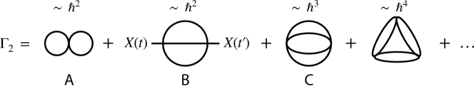
Figure 3: The leading order diagrams for $\Gamma_{2}$ in $\hbar$ expansion.

III.3 –‌

Basics of 2PI In Sec. III.1, we showed how to find the effective action for a quantum system in terms of the expectation values of its operators. The effective action can be generalized to also explicitly depend on the correlation functions of the theory. In that case, the stationary solution of $\Gamma$ yields also the equations of motion for the correlation functions [63]. The simplest case of these effective actions, which is used in this work, depends only on the 1-point and 2-point functions. For technical reasons that will be explained below, $\Gamma$ is called the 2-particle irreducible (2PI) effective action (EA) in this case. Keldysh formalism of the previous section allows us to efficiently calculate $\Gamma$. A brief description of the approach is given below, while a comprehensive introduction can be found in Ref. [62].

III.3.1 Basic Definitions

For simplicity, we use the toy model of a single particle in Eq. (30) in an anharmonic potential to pedagogically introduce the derivation of Dyson equations (DE) from the 2PI formalism. The potential is given by

$$V(x)=\frac{1}{2}\omega^{2}x^{2}+\frac{u}{4!}x^{4}.$$ (31)

We also re-scale $x$ such that $m\equiv 1$. In the next step, we introduce source terms by [62]

$$S\to S+\oint dt\,J_{s}(t)x_{s}(t)+\frac{1}{2}\oint\oint dt\,dt^{\prime}\,R(t,t^{\prime})x(t)x(t^{\prime}).$$ (32)

We further define the generating functional $\mathcal{W}[J,R]$ in terms of the trace of $\rho(t)$ in the presence of sources

$$e^{i\mathcal{W}}\equiv\int\mathcal{D}[x]e^{iS+i\int J\cdot xdt+\frac{i}{2}\int\int dtdt^{\prime}x\cdot R\cdot x}.$$ (33)

It is easy to show that

$$\frac{\delta\mathcal{W}}{\delta J(t)}=\expectationvalue{x(t)}\equiv X(t),$$ (34)

and that the connected 2-point correlation function, Eq. (24, can be obtained from

$$\frac{\delta\mathcal{W}}{\delta R(t,t^{\prime})}=\frac{1}{2}\Big{(}X(t)X(t^{\prime})+iG(t,t^{\prime})\Big{)}.$$ (35)

The effective action in terms of $X$ and $G$ is given by the Legendre transform of $\mathcal{W}$ [62]

$$\Gamma[X,G]=\mathcal{W}[J,R]-\oint dtJ(t)X(t)\\ -\frac{1}{2}\oint\oint dt\,dt^{\prime}\,R(t,t^{\prime})\Big{(}X(t)X(t^{\prime})+G(t,t^{\prime})\big{)}.$$ (36)

In principle, $J$ and $R$ have to be found in terms of $X$ and $G$ using Eqs. (34) and (35) and then be put into Eq. (36). However, a direct evaluation of the functional derivatives shows that

$$\frac{\delta\Gamma}{\delta X(t)} =-J(t)-\oint dt\,R(t,t^{\prime})X(t^{\prime}),$$ (37)

$$\frac{\delta\Gamma}{\delta G(t,t^{\prime})} =-\frac{i}{2}R(t^{\prime},t),$$ (38)

and therefore, in the absence of sources, the equations of motion are given by $\delta\Gamma/\delta X=\delta\Gamma/\delta G=0$ as expected.

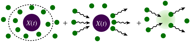
Figure 4: Schematic representation of different processes captured by the first few terms in the expansion of the 2PI effective action for a single quantum mechanical particle in an anharmonic potential. Green circles represent the excitations (’phonons’) generated on top of $X(t)$. Left panel: At the leading order (LO), the coupling of the classical mean field solution $X$ to fluctuations leads to time-dependent effective mass for $X$ and a time-dependent gap for fluctuations. The next-to-leading order (NLO) corrections take into account the generation and annihilation of fluctuations by the classical mean field solution $X$ (center panel) and their interactions (right panel), similar to the scattering of phonons from each other. These effects lead to dissipation and equilibration of the system in both mean field and fluctuation sectors.

The main complication of finding $\Gamma$ is the lack of explicit relations for $(J,R)$ in terms of $(X,G)$. Fortunately, a diagrammatic representation for $\Gamma$ exists whose derivation can be found in the literature [63, 62, 87]. The final result is given by

$$\Gamma[X,G]=S[X]-\frac{i}{2}\Tr\ln G^{-1}+\frac{i}{2}\Tr(G_{0}^{-1}G)+\Gamma_{2}.$$ (39)

For the anharmonic oscillator, $S$ is the action in (30) and $G_{0}$ is the connected Green’s function of the system given by $G_{0}(t_{c},t^{\prime}_{c})=-i\expectationvalue{\delta x(t_{c})\delta x(t^{\prime}_{c})}$ after we expand the action around the expectation value, $X$, of $x=X+\delta x$, and keep the result to quadratic order in $\delta x$. $G_{0}^{-1}$ is given by the kernel of the action for a particle in the potential of Eq. (31) after expanding the action around a classical solution $X$ and keeping terms up to quadratic order in $\delta x$

$$G_{0}^{-1}(t,t^{\prime})=\delta(t,t^{\prime})\quantity(-\partial_{t}^{2}-\omega^{2}-\frac{u}{4}X^{2}).$$ (40)

The trace terms in Eq. (39) describe the contribution of Gaussian fluctuations on top the classical solution given by $X$. Finally, the last term in (39) contains non-Gaussian contributions. It can be shown that [63, 62, 87] $\Gamma_{2}$ is given by the sum of all vacuum bubbles, e.g. Feynman diagrams without external legs, which cannot be split into disconnected parts by cutting at most two of their lines, hence the name ’two-particle irreducible’ (2PI) for the method. Some of the first few diagrams of $\Gamma_{2}$ are shown in Fig. 3. The diagrams in Fig. 3 are sorted in terms of their scaling with the Planck constant. The number of loops in each diagram determines the power $\hbar$ that diagram scales with [139, 140, 62, 141]. For instance, the first two diagrams in Fig. 3 are $\mathcal{O}(\hbar^{2})$ and the third one is $\mathcal{O}(\hbar^{3})$. This suggests an expansion of $\Gamma_{2}$ in powers of $\hbar$. The limit $\hbar\to 0$ corresponds to the classical solution, and by including higher order terms in $\hbar$ we take quantum effects into account. We again remark that this procedure is not a perturbative expansion. It is equivalent to a resummation of an infinite number of terms, as each Green’s function in Fig. 3 is renormalized by interactions and has to evaluated self-consistently. $\hbar$ is not always a good expansion parameter. For example, in many-body systems quantum effects can be amplified due to the many degrees of freedom strongly interacting with each other. In these situations, another control parameter for the expansion is required, such as the inverse of the number of particle species [61, 64, 62, 79] or the inverse of spin size, which we will use later in Section IV. For later reference, we give the expressions for diagrams in Fig. 3

$$\Gamma_{A} =+\frac{u}{8}\oint\quantity[G(t,t)]^{2}\,dt,$$ (41)

$$\Gamma_{B} =-\frac{u^{2}}{12}\oint\oint X(t)\quantity[G(t,t^{\prime})]^{3}X(t^{\prime})\,dt\,dt^{\prime},$$ (42)

$$\Gamma_{C} =+\frac{iu^{2}}{48}\oint\oint\quantity[G(t,t^{\prime})]^{4}\,dt\,dt^{\prime}.$$ (43)

III.3.2 Equations of Motion

The equations of motion are given by Eqs. (37) and (38). For an expansion of $\Gamma_{2}$ to third order in $\hbar$, we have for the dynamics of $X$

$$\big{(}\overbrace{\partial_{t}^{2}+\omega^{2}+\frac{u}{6}X^{2}}^{\sim\hbar^{0}}+\overbrace{\frac{iu}{2}G(t,t)}^{\sim\hbar}\big{)}X(t)=\\ \overbrace{\frac{u^{2}}{6}\oint\quantity[G(t,t^{\prime})]^{3}X(t^{\prime})\,dt^{\prime}}^{\sim\hbar^{2}}.$$ (44)

This equation is similar to the classical equation of motion for $X$ with extra terms that capture quantum corrections to the dynamics. The dynamics of $X$ can be imagined as the motion of a classical particle interacting with the fluctuations (also referred as ’phonons’ for pictorial purposes) around the mean field solution. At first order (left panel in Fig. 4), the effective mass of $X$ becomes time-dependent due to a shift given by $\delta\omega^{2}(t)=iuG(t,t)/2$. Furthermore, the fluctuation gap becomes dependent on $X$. Since $X$ changes with time, the fluctuation gap also becomes time-dependent, and $X$ acts as a coherent drive for fluctuations. Equivalently, the dynamics is approximated by a time-dependent Gaussian ansatz for the variational state in Eq. (9) [131], which is equivalent to the Bogoliubov approximation [101] for the dynamics. The effect of higher order corrections can be imagined as the incoherent creation and absorption of fluctuations by $X$ (middle panel of Fig. 4), given by the RHS of Eq. (44) as a memory term. The advantage of 2PI is that it takes into account these processes non-perturbatively by resumming their contributions to infinite order. The equation of motion for $G$ always has the following general form

$$G_{0}^{-1}G(t,t^{\prime})=\delta_{c}(t,t^{\prime})+\oint\Sigma(t,t^{\prime\prime})G(t^{\prime\prime},t^{\prime})\,dt^{\prime\prime},$$ (45)

known as the Dyson equation [101]. $\delta_{c}(t,t^{\prime})$ is the delta function for contour variables. $\Sigma$ is the self-energy functional and is defined as

$$\Sigma(t,t^{\prime})\equiv 2i\frac{\delta\Gamma_{2}}{\delta G(t^{\prime},t)}.$$ (46)

Pictorially, $\Sigma$ is obtained by removing a single line from diagrams in $\Gamma_{2}$. Evaluating $\Sigma$ and using Eq. (40) gives

$$-\Big{(}\partial_{t}^{2}+\omega^{2}+\frac{u}{2}X^{2}+\frac{iu}{2}G(t,t)\Big{)}G(t,t^{\prime})=\delta_{c}(t,t^{\prime})\\ +\oint\tilde{\Sigma}(t,t^{\prime\prime})G(t^{\prime\prime},t^{\prime})\,dt^{\prime\prime},$$ (47)

where we have separated the non-local part of $\Sigma$ as $\tilde{\Sigma}$. $\tilde{\Sigma}$ is the sum of $\Gamma_{B}$ and $\Gamma_{C}$ which are respectively obtained using the functional derivatives of $\Gamma_{B}$ and $\Gamma_{C}$ in Eqs. (42) and (43)

$$\tilde{\Sigma}(t,t^{\prime})=-\frac{iu^{2}}{2}X(t)\quantity[G(t,t^{\prime})]^{2}X(t^{\prime})-\frac{u^{2}}{6}\quantity[G(t,t^{\prime})]^{3}.$$ (48)

The last term in Eq. (48) describes the ’collisions’ between excitations (right panel of Fig. 4) and usually leads to redistribution of energy and thermalization of system at long times. Eqs. (44) and (47) are called Dyson equations [87, 101]. Usually, DE can be solved only approximately using analytical approaches. Approximate methods can usually access dynamics at early times, where a perturbative expansion around the initial state is valid, and near equilibrium, where time translation symmetry is approximately true. To capture far from equilibrium dynamics at all stages of the evolution we usually need to solve DE numerically without further approximations [62]. The latter approach has shown promising results for dynamics in various physical systems out of equilibrium [142, 65, 66, 67, 68, 69, 70, 73, 143, 75, 76, 77, 78, 79, 80, 81, 82, 144, 83, 145]).

III.3.3 Comparison with other approaches

There are various methods to explore many-body quantum dynamics theoretically and each one has its own advantages and shortcomings. Exact diagonalization (ED) gives accurate results but is often limited to very small system sizes, especially for open quantum systems where the size of the vector space grows even faster due to the necessity of working with mixed states. Methods based on matrix product states (MPS) [146] are mostly limited to one spatial dimension and systems with local interactions and weak entanglement. Among the most frequently used methods in the AMO community are cumulants expansion (CE) and truncated Wigner approximation (TWA) [147] together with its extension, discrete truncated Wigner approximation (DTWA) [148]. The main advantages of CE are simplicity and cheap computational cost. On the other hand, it is an uncontrolled approximation [149, 150]. There is no a priori knowledge of its domain of applicability before solving the equations and check the physical consistency of the results. Furthermore, to calculate correlation functions at different times in CE, one needs to resort to the quantum regression theorem [114, 151], which complicates the calculations. TWA approximates quantum dynamics with classical statistical mechanics by sampling the initial probability distribution function from the system’s initial wave function and subsequently, evolving the system according to the classical equations of motion. The advantage of TWA is that it is a controlled approximation, since it can be expressed as the leading order contribution in the expansion of dynamics in powers of $\hbar$, which turn out to be a weighted average of classical dynamics [147]. The drawback of TWA is its limitation to systems with weak quantum fluctuations and when quantum effects are not built up over time. For instance, TWA is unable to capture tunneling phenomena [147] even at the level of qualitative accuracy. While the calculation of non-local symmetric correlation functions is straightforward in TWA, to evaluate quantities such as response functions one needs to go to higher order terms in $\hbar$ [147], considerably increasing the required effort to use the method. In comparison to CE and TWA, 2PI can be used to perform controlled approximations, provided that a control parameter exists in the system. In this case, the 2PI action admits an expansion in powers of the control parameter [62]. For instance, this parameter can be $\hbar$, similar to the example given before, or inverse of the components of a vector field or in our case, the inverse of the spin amplitude per cluster and the number of photon modes to the number of clusters. Moreover, symmetric and anti-symmetric correlation functions are the quantities in terms of which the formalism is built and are the direct outcomes of calculations. 2PI also excels in capturing quantum effects, mainly because it involves a resummation of the perturbative expansion to infinite order. For instance, it has been used to study dynamics in strongly correlated systems of electrons [143, 152, 153] and phonons [145, 154] with non-Fermi liquid (NFL) behavior and critical fluctuations. 2PI works well also when small quantum effects are accumulated over time, leading to drastic changes in the system at long times such as in tunneling phenomena [65, 155]. Despite numerous advantages, 2PI has some limitations. First, the approximations that are usually made to retain only a subset of the diagrams in the effective action, such as $1/N$ expansions [64, 61, 62, 79], give qualitatively valuable results about the universal trend of the dynamics, but are not tailored to have quantitative accuracy, i.e., they are not suitable for a point-wise comparison with experimental data. Sometimes, one needs to make educated guesses about which diagrams have to be kept to capture a certain aspect of the physics which is of interest. The exception to these is working in the weak coupling or the dilute limit, where collisions can be incorporated perturbatively [101, 87]. Second, working with non-Gaussian initial states is difficult in 2PI as these require the inclusion of extra interaction vertices [62] that complicate the approximation. We emphasize that this restriction only holds for initial states. 2PI is not limited to Gaussian dynamics (such as second order cumulants) and in fact, captures non-Gaussian correlations generated over time after initializing the systems in a Gaussian state.

IV 2PI for Disordered Cavity-QED

Figure 5: The spin-photon interaction vertex after averaging over the disorder. The dashed line indicates the average $\overline{g_{\alpha,i}g_{\beta,j}}$.

$\Gamma_{2}\hskip 5.0pt\approx\hskip 5.0pt\underset{\mbox{\scalebox{1.0}{$\Gamma_{2}^{\mathrm{LO}}\sim N_{s}$}}}{\vbox{\hbox{\includegraphics[height=21.68231pt]{MF.png}}}}\hskip 5.0pt+$ $\underbrace{\Bigg{(}\vbox{\hbox{\includegraphics[height=34.69038pt]{melon.png}}}\hskip 2.0pt+\hskip 2.0pt\vbox{\hbox{\includegraphics[height=34.69038pt]{2.png}}}\hskip 2.0pt+\hskip 2.0pt\vbox{\hbox{\includegraphics[height=34.69038pt]{3.png}}}\hskip 2.0pt+\hskip 2.0pt\vbox{\hbox{\includegraphics[height=34.69038pt]{4.png}}}\hskip 2.0pt+\,\,\dots\Bigg{)}}_{\mbox{\scalebox{1.0}{$\Gamma_{2}^{\mathrm{NLO}}\sim N_{s}^{0}$}}}$

Figure 6: The leading-order and next-to-leading-order diagrams in the $1/N_{s}$ expansion of 2PI action.

IV.1 Keldysh Action for Spins

In order to treat Eq. (1) using field theory, we need a path integral representation for spin operators. Different spin representations include spin coherent state path integral and representations in terms of bosons or fermions [156]. In this work, we represent each spin-half operator in terms of three Majorana fermions $(\psi^{x},\psi^{y},\psi^{z})$ as [157, 158, 159, 160, 161, 162, 163, 164, 165, 166, 167, 168, 169] given by

$$\sigma^{\alpha}=-i\epsilon_{\alpha\beta\gamma}\psi^{\beta}\psi^{\gamma},\qquad\anticommutator{\psi^{\alpha}}{\psi^{\beta}}=\delta_{\alpha\beta},$$ (49)

where we have assumed summation over repeated indices. It is easy to check that (49) satisfies spin commutation relations $\commutator{\sigma^{\alpha}}{\sigma^{\beta}}=2i\epsilon_{\alpha\beta\gamma}\sigma^{\gamma}$. This representation was used by Refs. [168, 169] to study the onset of superradiance in the steady state of the Dicke model with different types of external baths. The Keldysh action for “free” spins, corresponding to the first term in Eq. (1) has two parts

$$S_{\sigma} =S_{\mathrm{B}}+S_{\Delta},$$ (50)

$$S_{\mathrm{B}} =\sum_{i}^{N}\sum_{\lambda}^{N_{s}}\sum_{\alpha}^{x,y,z}\oint\frac{i}{2}\psi^{\alpha}_{i\lambda}\partial_{t_{c}}\psi^{\alpha}_{i\lambda}\,dt_{c},$$ (51)

$$S_{\Delta} =\sum_{i}^{N}\sum_{\lambda}^{N_{s}}\oint i\Delta\psi^{x}_{i\lambda}\psi^{y}_{i\lambda}\,dt_{c},$$ (52)

where $S_{B}$ is the contribution of the Berry phase of spins to the action [170]. The action in Eq. (50) can be compactly written as

$$S_{\sigma}=\frac{1}{2}\sum_{i}^{N}\sum_{\lambda}^{N_{s}}\oint\Psi^{T}_{i\lambda}\hat{G}_{0}^{-1}\Psi_{i\lambda}\,dt_{c},$$ (53)

with $\Psi^{T}_{i\lambda}\equiv(\psi^{x}_{i\lambda},\psi^{y}_{i\lambda},\psi^{z}_{i\lambda})$. The inverse bare Green’s function for fermions $\hat{G}_{0}^{-1}$ is defined as

$$\hat{G}_{0}^{-1}\equiv\begin{bmatrix}i\partial_{t_{c}}&i\Delta&0\\ -i\Delta&i\partial_{t_{c}}&0\\ 0&0&i\partial_{t_{c}}\end{bmatrix}.$$ (54)

Finally, we define the fermion Green’s function and its diagrammatic representation as

$$iG_{i\lambda,j\lambda^{\prime}}^{\alpha,\beta}(t,t^{\prime})\equiv\expectationvalue{\psi^{\alpha}_{i\lambda}(t)\psi^{\beta}_{j\lambda^{\prime}}(t^{\prime})}:\includegraphics{psipsi.pdf}.$$ (55)

Note that $G$ is the dressed fermion Green’s function.

IV.2 Keldysh Action for Photon Sector

The dissipative Keldysh action for photons can be obtained directly from the Liouvillian, by following the prescription given in Ref. [88]

$$S_{\mathrm{ph}}=\int\big{[}\bar{a}_{+}\quantity(i\partial_{t}-\omega_{c}+i\kappa)a_{+}-\bar{a}_{-}\quantity(i\partial_{t}-\omega_{c}-i\kappa)a_{-}\\ -2i\kappa\bar{a}_{-}a_{+}\big{]}\,dt.$$ (56)

Since the spin-photon coupling in Eq. (1) depends on the combination $(a+a^{\dagger})$ of photon operators, dealing with interactions is simpler when we make the following transformation to real-valued photon fields $(\phi,\pi)$ given by:

$$a_{\pm}=\sqrt{\frac{\omega_{c}}{2}}\quantity(\phi_{\pm}+i\frac{\pi_{\pm}}{\omega_{c}}).$$ (57)

Substitution in Eq. (56) gives

$$S_{\mathrm{ph}}=\frac{1}{2}\sum_{\alpha}^{M}\int\Phi_{\alpha}^{T}\hat{D}_{0}^{-1}\Phi_{\alpha}\,dt,$$ (58)

where $\Phi_{\alpha}^{T}\equiv\quantity(\phi_{\alpha+},\pi_{\alpha+},\phi_{\alpha-},\pi_{\alpha-})$ and $\hat{D}_{0}^{-1}$ is a $4\times 4$ matrix defined as

$$\hat{D}_{0}^{-1} =\begin{bmatrix}\quantity(\hat{D}_{0}^{-1})^{++}&\quantity(\hat{D}_{0}^{-1})^{+-}\\ \quantity(\hat{D}_{0}^{-1})^{-+}&\quantity(\hat{D}_{0}^{-1})^{--}\end{bmatrix},$$ (59)

$$\quantity(\hat{D}_{0}^{-1})^{++} =\begin{bmatrix}-\omega_{c}^{2}+i\kappa\omega_{c}&-\partial_{t}\\ \partial_{t}&-1+i\frac{\kappa}{\omega_{c}}\end{bmatrix},$$ (60)

$$\quantity(\hat{D}_{0}^{-1})^{+-} =\begin{bmatrix}-i\kappa\omega_{c}&-\kappa\\ \kappa&-i\frac{\kappa}{\omega_{c}}\end{bmatrix},$$ (61)

$$\quantity(\hat{D}_{0}^{-1})^{-+} =\begin{bmatrix}-i\kappa\omega_{c}&\kappa\\ -\kappa&-i\frac{\kappa}{\omega_{c}}\end{bmatrix},$$ (62)

$$\quantity(\hat{D}_{0}^{-1})^{--} =\begin{bmatrix}\omega_{c}^{2}+i\kappa\omega_{c}&\partial_{t}\\ -\partial_{t}&1+i\frac{\kappa}{\omega_{c}}\end{bmatrix}.$$ (63)

Photon Green’s functions are defined according to

$$iD^{\rho,\rho^{\prime}}_{\alpha,\beta}(t,t^{\prime})\equiv\expectationvalue{\Phi^{\rho}_{\alpha}(t)\Phi^{\rho^{\prime}}_{\beta}(t^{\prime})}_{c},$$ (64)

where $\rho,\rho^{\prime}=(\phi,\pi)$. We will see that only the $D^{\phi\phi}$ component appears explicitly in the diagrams for the effective action and self-energies. Hence, only $D^{\phi\phi}$ requires a diagrammatic representation which is given by

$$iD^{\phi\phi}_{\alpha,\beta}(t,t^{\prime})=\expectationvalue{\phi_{\alpha}(t)\phi_{\beta}(t^{\prime})}_{c}:\includegraphics{phiphi.pdf}.$$ (65)

IV.3 Spin-Photon Interaction

Using the conventions introduced above, the Keldysh action for the interaction term reads

$$S_{\mathrm{int}}=2i\sqrt{\frac{2\omega_{c}}{(N+M)N_{s}}}\sum_{\alpha,i,\lambda}\oint dt_{c}\,g_{\alpha i}\phi_{\alpha}\psi^{y}_{i\lambda}\psi^{z}_{i\lambda}.$$ (66)

In principle, we can proceed by taking the average of the Keldysh action over the random couplings $g_{\alpha i}$. This yields an effective interaction defined by $e^{iS_{\mathrm{eff}}}=\overline{e^{iS_{\mathrm{int}}}}$ where

$$S_{\mathrm{eff}}\equiv-\frac{4ig^{2}\omega_{c}}{(N+M)N_{s}}\sum_{\alpha,i}\sum_{\lambda,\lambda^{\prime}}\oint\oint dt_{c}\,dt^{\prime}_{c}\,\phi_{\alpha}(t_{c})\phi_{\alpha}(t^{\prime}_{c})\\ \times\psi^{y}_{i\lambda}(t_{c})\psi^{z}_{i\lambda}(t_{c})\psi^{y}_{i\lambda^{\prime}}(t^{\prime}_{c})\psi^{z}_{i\lambda^{\prime}}(t^{\prime}_{c}).$$ (67)

We have assumed that the initial state is not correlated with disorder profile (see comments in Sections IV.4 and IV.5 for more details). The diagrammatic form of $S_{\mathrm{eff}}$ is given in Fig. 5. To have a systematic and controlled approximation in $1/N_{s}$ that captures the frustrated nature of the problem, we have to keep an infinite subset of 2PI diagrams shown in Fig. 6. A closed form for the corresponding summation can be found, as shown for example for quantum $O(N)$ model in Refs. [64, 61, 62, 84]. An easier approach is the auxiliary field method [64, 61, 62], based on the Hubbard-Stratonovich (HS) transformation [101, 11, 79, 82]. HS transformation finds various applications in the study of collective effects in many body systems such as plasmons [11], superconductivity [11, 171], superfluidity [170] and quantum spin liquids [172]. The basic idea is to introduce a new field which we label as $\chi$, that mediates the original interaction in $S_{\mathrm{int}}$. In our case, $\chi$ decouples the interaction between spins and cavity modes as diagrammatically illustrated in Fig. 7a. The action of $\chi$ and its coupling to other degrees of freedom are given by (see Appendix A for a mathematical derivation)

$$S_{\mathrm{int}}\to S_{\chi}+S_{\chi\psi}+S_{g\chi\phi},$$ (68)

where $S_{\chi}$ is the action of the HS defined as

$$S_{\chi}\equiv\frac{1}{2}\sum_{\alpha,\beta}^{M}\sum_{i,j}^{N}\sum_{\sigma,\sigma^{\prime}}^{1,2}\oint\oint dt_{c}\,dt^{\prime}_{c}\,\\ \times\chi^{\sigma}_{\alpha i}(t_{c})\cdot\quantity(\hat{W}^{-1}_{0})^{\sigma,\sigma^{\prime}}_{\alpha i,\beta j}(t_{c},t^{\prime}_{c})\cdot\chi^{\sigma^{\prime}}_{\beta j}(t^{\prime}_{c}).$$ (69)

We name $\chi$ as the Ising field, as it mediates the Ising-type interaction amongst spins as we will see below. $\chi$ is a two-component real valued scalar field defined as

$$\vec{\chi}_{\alpha i}\equiv\quantity(\chi^{1}_{\alpha i},\chi^{2}_{\alpha i}),$$ (70)

together with its inverse bare Green’s function

$$\quantity(\hat{W}^{-1}_{0})^{\sigma,\sigma^{\prime}}_{\alpha i,\beta j}(t_{c},t^{\prime}_{c})\equiv\sqrt{N+M}\delta_{\alpha\beta}\delta_{ij}\quantity(\sigma^{x})_{\sigma\sigma^{\prime}}\delta(t_{c},t^{\prime}_{c}),$$ (71)

and its full Green’s function

$$iW_{\alpha i,\beta j}^{\sigma,\sigma^{\prime}}(t,t^{\prime})\equiv\expectationvalue{\chi^{\sigma}_{\alpha i}(t)\chi^{\sigma^{\prime}}_{\beta j}(t^{\prime})}_{c}:\includegraphics{chichi.pdf}.$$ (72)

Note that the “free” part of the action for the Ising field $S_{\chi}$ is local in time and does not contain any time derivatives of $\chi$. This makes the equations of motion for $\chi$ algebraic rather than differential. The latter is the generic case where the equations of motion for correlation functions form a system of coupled differential equations, and adiabatic elimination is equivalent to approximately ignoring the time derivatives of some of the dynamical variables, which are assumed to have a quick response compared to other timescales in the system. For the HS field, adiabatically eliminating $\chi$ is exact, which is equivalent to taking the Gaussian integral over $\chi$ in Eq. (69), and the result is given by $S_{\mathrm{int}}$ in Eq. (66). The next term in Eq. (68) is $S_{\chi\psi}$ which describes the coupling of fermions to the first component of $\chi$:

$$S_{\chi\psi}\equiv-\frac{2i}{\sqrt{N_{s}}}\sum_{\alpha,i,\lambda}\oint dt_{c}\,\chi^{1}_{\alpha i}\psi^{y}_{i\lambda}\psi^{z}_{i\lambda},$$ (73)

and $S_{g\chi\phi}$ describes the disordered interaction of photons with the second component of $\chi$

$$S_{g\chi\phi}\equiv\sqrt{2\omega_{c}}\sum_{\alpha,i}\oint dt_{c}\,\chi^{2}_{\alpha i}g_{\alpha i}\phi_{\alpha}.$$ (74)

The diagrammatic representations of the original vertex in Eq. (66) and the transformed ones (Eqs. (73) and (74) are given in Fig. 7a. We will show later that the two components of the Ising field correspond to different physical quantities. As will be shown in Section IV.8.1, $\chi^{1}$ is related to the effective magnetic field each cluster experiences and $\chi^{2}$ is connected to magnetization. Similarly, the Green’s functions of Ising fields are not just mathematical objects and have physical meanings. $W$ can be expressed in terms of the original Green’s functions as shown in Fig. 7c. $W^{22}$ is related to the spin-spin correlation function or equivalently, the 4-point function of Majorana fermions

$$\expectationvalue{S^{x}_{i}(t)S^{x}_{i}(t^{\prime})}=-4\sum_{\lambda,\lambda^{\prime}}^{N_{s}}\expectationvalue{\psi^{y}_{i\lambda}(t)\psi^{z}_{i\lambda}(t)\psi^{y}_{i\lambda^{\prime}}(t^{\prime})\psi^{z}_{i\lambda^{\prime}}(t^{\prime})}$$ (75)

whose leading order expansion is given by the same set of diagrams as $W^{22}$ in Fig. 7c, up to multiplication by an overall constant, as given by Eq. (118). Therefore, spin-spin correlation functions are natural byproducts of our formalism. Therefore, there is no need to solve the Bethe-Salpeter equations to obtain 4-point functions of fermions, usually a cumbersome task particularly for out of equilibrium systems [79, 173, 86].

(a)

(b)

(c)

Figure 7: (a) The original interaction vertex and the decoupled interactions after HS transformation. (b) The effective interaction between photons and the Ising field after disorder averaging. (c) Diagrammatic representation of the Ising (HS) field propagators. The appearing fermion and photon lines are assumed to be renormalized by interactions. Thick curls are the dressed Green’s functions of $\chi$ and thin curls are the bare propagators of $\chi$ and only have constant off-diagonal elements. $W^{22}$ coincides with spin-spin correlation function, up to an overall multiplicative factor.

IV.4 Disorder Averaging

We can now take the average over the disordered couplings. In the Keldysh formalism, the average can be taken without resorting to the replica trick [101]. The only term in the action depending on $g$ is $S_{g\chi\phi}$. The effective interaction after disorder averaging is given by $e^{iS_{\chi\phi}}=\overline{e^{iS_{g\chi\phi}}}$, where

$$S_{\chi\phi}=ig^{2}\omega_{c}\sum_{\alpha i}\oint\oint dt_{c}\,dt^{\prime}_{c}\,\chi^{2}_{\alpha i}(t_{c})\phi_{\alpha}(t_{c})\chi^{2}_{\alpha i}(t^{\prime}_{c})\phi_{\alpha}(t^{\prime}_{c}),$$ (76)

is shown diagrammatically in Fig. 7b. We have to make an important remark about the process of disorder averaging. In obtaining Eq. (76) we have assumed that the initial state of the system is not correlated with the disorder. This is valid for the initial states we consider in this paper. However, to study phenomena such as associative memory in multi-mode cavity QED [121, 122, 124, 108, 174, 43], where a significant overlap of the initial spin configuration is required for memory retrieval, one has to assume that the initial state depends on $g_{\alpha i}$. In that case, disorder averaging will generate more terms than Eq. (76), which couple the initial state to the interaction vertex in Eq. (74).

IV.5 Symmetry Considerations

The symmetry structure of the model helps us to simplify the study of its dynamical response. Originally, the Hamiltonian in Eq. (1) is invariant only under a global $Z_{2}$ transformation that maps all spins and cavity modes simultaneously according to

$$\sigma^{x}_{i\lambda}\to-\sigma^{x}_{i\lambda},\qquad a_{\alpha}\to-a_{\alpha}.$$ (77)

According to the language of Ref. [175, 88, 176, 177], in the absence of photon loss this is a quantum symmetry of the system with a conserved $Z_{2}$ charge. A quantum symmetry is a symmetry of the fields on each individual Keldysh contour, while a classical symmetry is the invariance of the Keldysh action under a simultaneous transformation of the fields on forward and backward contours [88]. With photon loss, the quantum symmetry is demoted to a classical symmetry without a conserved charge. However, starting from a symmetric initial state, a classical symmetry still guarantees that the symmetry will remain unbroken in the absence of symmetry breaking perturbations. The symmetry structure of the model is enriched after disorder averaging and using the fermion representation in Eq. (49). It can be easily verified that the disorder-averaged Keldysh action has the following sets of symmetries

1. A local $Z_{2}$ gauge symmetry under the transformation

   $$\vec{\psi}_{i\lambda}\to-\vec{\psi}_{i\lambda},$$ (78)

   which holds for each spin separately. This symmetry is an artifact of representing spins in terms of quadratic fermion operators, and is not physical. The initial state or external forces cannot break this symmetry. The important consequence of this symmetry is that

   $$G^{\alpha,\beta}_{i\lambda,j\lambda^{\prime}}\propto\delta_{ij}\delta_{\lambda\lambda^{\prime}}.$$ (79)

2. A $Z_{2}$ symmetry for each separate cluster $i$ and Ising fields coupled to it:

   $$\sigma^{x}_{i\lambda} \to-\sigma^{x}_{i\lambda},\quad(\lambda=1,...,N_{s}),$$ (80)

   $$\chi^{\sigma}_{\alpha i} \to-\chi^{\sigma}_{\alpha i},\quad(\sigma=1,2),\quad(\alpha=1,...,M).$$ (81)

   (81) holds because the effective interaction in Eq. (76) is quadratic in $\chi$. This symmetry is a classical symmetry with no conserved quantities.

3. A $Z_{2}$ symmetry of each photon mode given by

   $$\phi_{\alpha}\to-\phi_{\alpha},\quad\pi_{\alpha}\to-\pi_{\alpha}.$$ (82)

   This symmetry is also a result of $S_{\chi\phi}$ being quadratic in photon fields and is a weak symmetry. This symmetry implies that

   $$D_{\alpha,\beta}^{\rho,\rho^{\prime}}\propto\delta_{\alpha\beta}.$$ (83)

We see that the $Z_{2}$ symmetries of spin and photon sectors are decoupled. This means that, even if the initial state of spins breaks the symmetry, no photon coherence will be generated ($\overline{\expectationvalue{a_{\alpha}(t)}}=0$). On the other hand, a finite value for $\sigma^{x}_{i\lambda}$ results in a finite value for $\chi^{1,2}_{\alpha i}$. We again remark that the above arguments hold true only if the initial state of the system is not correlated with the disorder pattern, such that Eq. (76) is the only outcome of disorder averaging. Otherwise, a $Z_{2}$ broken initial state can in principle break the $Z_{2}$ symmetry of some of the photon modes. This happens for example, if the initial spin configuration has a strong overlap with a single disorder pattern corresponding to the photon mode $\alpha$, such that

$$\lim_{N\to\infty}\frac{1}{NN_{s}}\absolutevalue{\sum_{i}^{N}\sum_{\lambda}^{N_{s}}\expectationvalue{\sigma^{x}_{i\lambda}}_{0}g_{\alpha i}}>0,$$ (84)

or if a symmetry breaking perturbation that favors a single pattern such as

$$\delta H=\epsilon\sum_{i,\lambda}g_{\alpha,i}\sigma^{x}_{i\lambda},$$ (85)

is applied to the system. In this case, one expects that for sufficiently small $M/N$, the pattern $\alpha$ to be activated and retrieved [122, 108]. For the fully polarized initial states of spins considered in this problem and in the thermodynamic limit, we can safely take $\overline{\expectationvalue{\phi_{\alpha}(t)}}=0$ throughout the evolution. Even starting from a state with $\expectationvalue{\phi}\neq 0$, its value will decay to zero as it cannot align itself with any of the disorder patterns.

IV.6 2PI Action

The 2PI action for the model given above is a functional of fermion, photon and Ising field correlation functions together with the expectation values of Ising fields and has the general form similar to Eq. (39) given by

$$\Gamma\quantity[\tilde{\chi},G,D,W]=S_{\chi}\quantity[\chi]+\frac{i}{2}\Tr\ln G-\frac{i}{2}\Tr\quantity(G_{0}^{-1}G)\\ -\frac{i}{2}\Tr\ln D+\frac{i}{2}\Tr\quantity(D^{-1}_{0}D)-\frac{i}{2}\Tr\ln W\\ +\frac{i}{2}\Tr\quantity(W^{-1}_{0}W)+\Gamma_{2}\quantity[\tilde{\chi},G,D,W].$$ (86)

The expressions for $S_{\chi}$, $G_{0}$, $D_{0}$ and $W_{0}$ were respectively given in Eqs. (69), (54), (59) and (71). $\tilde{\chi}$ is the expectation value of the Ising field

$$\tilde{\chi}^{\sigma}_{\alpha i}(t)\equiv\overline{\expectationvalue{\chi^{\sigma}_{\alpha i}(t)}},$$ (87)

shown by a black circle connected to a spring in (Fig. 8a). The last term in Eq. (86) captures interactions and as we mentioned in Sec. III.3, is given by the sum of 2PI diagrams. In order to systematically expand $\Gamma_{2}$, we need to specify how the expectation values and Green’s functions of the Ising field scale with parameters of the system. According to Eq. (71) to the leading order in $(N+M)^{-1}$ we have

$$W^{12}_{i\alpha,j\beta}\sim\delta_{ij}\delta_{\alpha\beta}\,\mathcal{O}\quantity(\frac{1}{\sqrt{N+M}}),$$ (88)

The diagonal elements $W^{11}$ and $W^{22}$ are zero at the bare level in Eq. (69). However, they become non-zero when the couplings of $\chi$ to $\psi$ and $\phi$ are taken into account (Fig. 7c). For $W^{22}$ we have

$$W^{22}_{i\alpha,j\beta}\sim\delta_{ij}\delta_{\alpha\beta}\,\mathcal{O}\quantity(\frac{1}{N+M}).$$ (89)

As will be shown later, $W^{11}$ has a sub-leading term due to interactions which contributes at leading order when it is summed over photon modes

$$W^{11}_{\alpha\beta}\sim\delta_{ij}\delta_{\alpha\beta}\,\mathcal{O}\quantity(\frac{1}{N+M})\\ +\delta_{ij}(1-\delta_{\alpha\beta})\,\mathcal{O}\quantity(\frac{1}{(N+M)^{2}}).$$ (90)

Furthermore, $\tilde{\chi}$ will have the following scalings (Eqs. (113) and (112))

$$\tilde{\chi}^{1}\sim\mathcal{O}\quantity(\frac{\sqrt{N_{s}}}{N+M}),\quad\tilde{\chi}^{2}\sim\mathcal{O}\quantity(\sqrt{\frac{N_{s}}{N+M}}).$$ (91)

At last, the fermion-Ising vertex in Eq. (73) has

$$S_{\chi\psi}\sim\frac{1}{\sqrt{N_{s}}}.$$ (92)

We now have all of the necessary ingredients to perform a systematic expansion of $\Gamma_{2}$.

IV.7 Diagrammatic Evaluation of 2PI Action

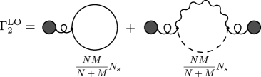
(a)

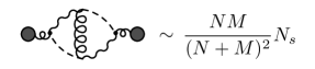
(b)

Figure 8: (a) The leading-order contribution of interactions to 2PI action. The dashed line in the right diagram is not a Green’s function and cannot be cut. (b) A diagram which linearly scales with $N_{s}$ but is not extensive and neglected. Black circles connected to springs represent the expectation value of Ising field $\chi$.

We are interested in the thermodynamic limit of the system in Eq. (1) where $N,M\to\infty$ while the ratio $\eta=M/N$ is kept fixed. Moreover, the number of spins per cluster $N_{s}$ is assumed to be larger than one and will play the role of the control parameter for the expansion. Also, we assume that $N_{s}\ll N$, which is a valid assumption in the thermodynamic limit of the problem. Similar to the quantum anharmonic oscillator considered in Section III, the interaction part of the 2PI action, given by $\Gamma_{2}$ in Eq. (86), admits a diagrammatic expansion in terms of the connected vacuum bubbles of the theory which cannot be split into half by cutting one or two of their Green’s function lines, also known as two-particle irreducible (2PI) graphs. Below, we will classify these diagrams for our system as leading-order (LO) terms

$$\Gamma_{2}^{\mathrm{LO}}\sim N_{s},$$ (93)

and next-to-leading-order (NLO) terms

$$\Gamma_{2}^{\mathrm{NLO}}\sim N_{s}^{0},$$ (94)

and higher order terms which are ignored in this work. We will also ignore terms which are sub-extensive. The following discussion will also elucidate how the parameter controlling the strength of quantum fluctuations, $N_{s}$, enters naturally in the field theory description and in the DE derived from it. This is one of the key merits of the approach, at variance with more numerical oriented methods which have to deal with growing computational complexity as $N_{s}$ is decreased.

IV.7.1 Leading-order contributions

The LO terms have linear scaling with $N_{s}$ and at the same time, scale extensively with system size. Two of these diagrams exist and both involve the expectation values of Ising fields, as shown in Fig. 8a. Their mathematical expressions are given by

$$\Gamma_{2}^{\mathrm{LO}}=\frac{2}{\sqrt{N_{s}}}\sum_{\alpha}^{M}\sum_{i}^{N}\sum_{\lambda}^{N_{s}}\oint dt_{c}\,\tilde{\chi}^{1}_{\alpha i}(t_{c})G^{y,z}_{i\lambda,i\lambda}(t_{c},t_{c})\\ -g^{2}\omega_{c}\sum_{\alpha}^{M}\sum_{i}^{N}\oint\oint dt_{c}\,dt^{\prime}_{c}\,\tilde{\chi}^{2}_{\alpha i}(t_{c})D_{\alpha,\alpha}^{\phi\phi}(t_{c},t^{\prime}_{c})\tilde{\chi}^{2}_{\alpha i}(t^{\prime}_{c}).$$ (95)

Note that the disorder (dashed) line in Fig. 8a cannot be cut, as it is a part of the disorder averaged interaction vertex in Fig. 7b. Accordingly, the right diagram in Fig. 8a is not 2-particle reducible. It can be shown, by solving the resulting equations of motion derived from Eq. (95), that the LO terms describe a dynamical mean field interaction of spin expectation values $\overline{\expectationvalue{\sigma^{x}}}$ mediated by photons through their response function (see Section V.1). Therefore, the LO contribution describes the LMG coupling in Eq. (5) with the inclusion of retardation effects due to photon dynamics. We note that there are other terms that scale linearly with $N_{s}$, such as the one given in Fig. 8b, but all of them scale non-extensively with system size and can be neglected in the thermodynamic limit.

IV.7.2 Next-to-leading-order contributions

Figure 9: Next-to-leading-order contributions to 2PI action.

The NLO diagrams do not scale with $N_{s}$ but still scale linearly with the number of clusters $N$. There are two NLO diagrams shown in Fig. 9 and their formulae are given by

$$\Gamma_{2}^{\mathrm{NLO}}=-\frac{2}{N_{s}}\sum_{\alpha,\beta}^{M}\sum_{i}^{N}\sum_{\lambda}^{N_{s}}\oint\oint dt_{c}\,dt^{\prime}_{c}\,W^{11}_{\alpha i,\beta i}(t_{c},t^{\prime}_{c})\\ \times\Big{(}G^{y,z}_{i\lambda}(t_{c},t^{\prime}_{c})G^{z,y}_{i\lambda}(t_{c},t^{\prime}_{c})-G^{y,y}_{i\lambda}(t_{c},t^{\prime}_{c})G^{z,z}_{i\lambda}(t_{c},t^{\prime}_{c})\Big{)}\\ -ig^{2}\omega_{c}\sum_{\alpha}^{M}\sum_{i}^{N}\oint\oint dt_{c}\,dt^{\prime}_{c}\,W^{22}_{\alpha i,\alpha i}(t_{c},t^{\prime}_{c})D^{\phi\phi}_{\alpha\alpha}(t_{c},t^{\prime}_{c}).$$ (96)

The rest of the terms in $\Gamma_{2}$ are either next-to-next-to-leading-order (NNLO) in $1/N_{s}$ or scale sub-extensively with system size (Fig. 10). In this work we neglect these terms and take

$$\Gamma_{2}\approx\Gamma_{2}^{\mathrm{LO}}+\Gamma_{2}^{\mathrm{NLO}}.$$ (97)

Figure 10: Some of the neglected diagrams in this work which appear after NLO terms. The left diagram is sub-extensive in system size and the rest are NNLO in $1/N_{s}$.

It is worth showing which diagrams we are keeping in terms of the original action prior to HS transformation (Fig. 6). As mentioned before, the LO part describes a retarded self-interaction of the spin expectation value expressed in terms of fermion Green’s function (according to Eq. 49)

$$\overline{\expectationvalue{\sigma^{x}}}=2G_{-+}^{z,y}(t,t),$$ (98)

given by closed loops in the first term of Fig. 6, within the same cluster and mediated by photons. In the regime of fast photons and at steady state, this reduces to the ferromagnetic interaction in Eq. 6. For NLO terms, the two diagrams in Fig. 9 are equivalent to the sum of an infinite number of diagrams in the original representation of the theory, shown in the brackets of Fig. 6. This can be verified by plugging the diagrammatic expression of $W$ given in Fig. 7c into the diagrams of Fig. 9, and subsequently substitute the lines for bare $W$ with simple dots, as the latter is just a constant. This infinite series is a byproduct of disordered couplings. For the Dicke model without disorder (see Appendix E), only the first NLO diagram would contribute since in the absence of disorder, dashed lines would disappear. This makes the rest of NLO diagrams 2-particle-reducible and hence, forbidden in the expansion of $\Gamma_{2}$.

IV.8 Equations of Motion

The equations of motion for Green’s functions and field expectation values are obtained similarly to Eqs. (37) and (38) in the absence of sources as

$$\frac{\delta\Gamma}{\delta\tilde{\chi}^{\sigma}_{\alpha i}(t)}=0,\qquad\frac{\delta\Gamma}{\delta W^{\sigma\sigma^{\prime}}_{\alpha i,\beta j}(t_{c},t^{\prime}_{c})} =0,$$ (99)

$$\frac{\delta\Gamma}{\delta D^{\rho\rho^{\prime}}_{\alpha,\beta}(t_{c},t^{\prime}_{c})}=0,\qquad\frac{\delta\Gamma}{\delta G^{\alpha\beta}_{i\lambda,j\lambda^{\prime}}(t_{c},t^{\prime}_{c})} =0.$$ (100)

After taking functional derivatives of Eq. (86), we see that the equations of motion for Green’s functions can always be cast compactly as

$$\hat{G}^{-1} =\hat{G}_{0}^{-1}-\hat{\Sigma},$$ (101)

$$\hat{D}^{-1} =\hat{D}_{0}^{-1}-\hat{\Pi},$$ (102)

$$\hat{W}^{-1} =\hat{W}_{0}^{-1}-\hat{\Omega},$$ (103)

known as Dyson equations [62, 87, 101]. The matrices $\hat{\Sigma}$, $\hat{\Pi}$ and $\hat{\Omega}$ are fermion, photon and Ising field self-energies, respectively. They are given in terms of the functional derivatives of $\Gamma_{2}$ as

$$\Sigma^{\alpha,\beta}_{i\lambda,j\lambda^{\prime}}(t_{c},t^{\prime}_{c}) \equiv-2i\frac{\delta\Gamma_{2}}{\delta G^{\beta,\alpha}_{j\lambda^{\prime},i\lambda}(t^{\prime}_{c},t_{c})},$$ (104)

$$\Pi^{\rho,\rho^{\prime}}_{\alpha,\beta}(t_{c},t^{\prime}_{c}) \equiv+2i\frac{\delta\Gamma_{2}}{\delta D^{\rho^{\prime},\rho}_{\beta,\alpha}(t^{\prime}_{c},t_{c})},$$ (105)

$$\Omega^{\sigma,\sigma^{\prime}}_{\alpha i,\beta j}(t_{c},t^{\prime}_{c}) \equiv+2i\frac{\delta\Gamma_{2}}{\delta W^{\sigma^{\prime},\sigma}_{\beta j,\alpha i}(t^{\prime}_{c},t_{c})}.$$ (106)

Due to their large size, the expanded forms of Eqs. (101-103), required for numerically solving them, are given in Appendix B. We will only mention the important details here. The fermion and photon Green’s functions will be diagonal in the spin-site and photon-mode bases, respectively. Due to permutation symmetry [19, 20, 178] we also have

$$G^{\alpha,\beta}_{i\lambda,j\lambda^{\prime}}(t_{c},t^{\prime}_{c}) =\delta_{ij}\delta_{\lambda\lambda^{\prime}}G^{\alpha,\beta}(t_{c},t^{\prime}_{c}),$$ (107)

$$D^{\rho,\rho^{\prime}}_{\alpha,\beta}(t_{c},t^{\prime}_{c}) =\delta_{\alpha\beta}D^{\rho,\rho^{\prime}}(t_{c},t^{\prime}_{c}).$$ (108)

The same is true for their self-energies. The Ising field’s Green’s function and its self-energy will acquire off-diagonal elements only in the photon indices. Due to the emergent permutation symmetry after disorder averaging, all diagonal elements of $W$ and $\Omega$ are the same. This holds also for the off-diagonal elements of $W$ and $\Omega$:

$$W^{\sigma,\sigma^{\prime}}_{\alpha i,\alpha j}(t_{c},t^{\prime}_{c}) =\delta_{ij}V^{\sigma,\sigma^{\prime}}(t_{c},t^{\prime}_{c}),$$ (109)

$$W^{\sigma,\sigma^{\prime}}_{\alpha i,\beta j}(t_{c},t^{\prime}_{c}) =\delta_{ij}U^{\sigma,\sigma^{\prime}}(t_{c},t^{\prime}_{c}),\quad\alpha\neq\beta.$$ (110)

A similar argument applies to $\tilde{\chi}$, and it has the same value for all sites and photon modes:

$$\tilde{\chi}^{\sigma}_{\alpha i}(t)=\tilde{\chi}^{\sigma}(t)$$ (111)

We proceed similarly to the previous section. We find the equations of motion at LO first and then consider the NLO corrections.

IV.8.1 Equations of motion at leading-order (LO)

For $\tilde{\chi}$, one always finds that it has the same value on forward and backward Keldysh contours, as it should be since these are classical variables. From Eqs. (95) and (99) we have

$$\frac{\delta\Gamma^{\mathrm{LO}}}{\delta\tilde{\chi}^{1}}=0\to\tilde{\chi}^{2}(t)=-2\sqrt{\frac{N_{s}}{N+M}}G_{-+}^{y,z}(t,t),$$ (112)

$$\frac{\delta\Gamma^{\mathrm{LO}}}{\delta\tilde{\chi}^{2}}=0\to\tilde{\chi}^{1}(t)=\frac{2g^{2}\omega_{c}}{\sqrt{N+M}}\int_{0}^{t}dt^{\prime}\,D_{R}^{\phi\phi}(t,t^{\prime})\tilde{\chi}^{2}(t^{\prime}),$$ (113)

where $D_{R}^{\phi\phi}$ is the photon response function defined as (for details see Appendix B)

$$D_{R}^{\phi\phi}(t,t^{\prime})\equiv-i\Theta(t-t^{\prime})\overline{\expectationvalue{\commutator{\hat{\phi}(t)}{\hat{\phi}(t^{\prime})}}},$$ (114)

which describes the response of the photons to an external linear perturbation. Note that the time variables used in Eq. (114) are normal variables and are not defined on the time contour. Substituting (112) into (113) gives

$$\tilde{\chi}^{1}(t)=-\frac{4g^{2}\omega_{c}\sqrt{N_{s}}}{N+M}\int_{0}^{t}dt^{\prime}\,D_{R}^{\phi\phi}(t,t^{\prime})G_{-+}^{y,z}(t^{\prime},t^{\prime}),$$ (115)

in agreement with the scaling relations for $\tilde{\chi}$ given in Eq. (91). For $\Sigma$ we have at the leading order

$$\Sigma_{\mathrm{LO}}^{\alpha,\beta}(t_{c},t^{\prime}_{c})=\parbox{34.14322pt}{\includegraphics[height=433.62pt]{Sigma_LO.pdf}}=-\frac{2iM}{\sqrt{N_{s}}}\epsilon_{x\alpha\beta}\delta(t_{c},t^{\prime}_{c})\tilde{\chi}^{1}(t_{c}).$$ (116)

The temporally local elements of fermion self-energy describe the effective magnetic field spins experience due to interactions. Accordingly, Eq. (116) describes a time-dependent magnetic field $B_{x}$ in the $\hat{x}$-direction experienced by each spin. This sheds light on the physical meaning of the first component of the HS field: it is the magnetic field experienced by each spin and its Green’s functions give the fluctuations of this field. This could be inferred also from Eq. (73) which describes the coupling of $\sigma^{x}=-2i\psi^{z}\psi^{y}$ to $\chi_{1}$. Similarly, Eqs. (112) and (98) relate $\chi^{2}$ to $\expectationvalue{\sigma^{x}}$ as

$$\overline{\expectationvalue{S^{x}_{i}(t)}}=-\sqrt{(N+M)N_{s}}\,\tilde{\chi}^{2}(t)/2.$$ (117)

Furthermore, it can be shown that $W^{22}$ is related to the 2-point correlation function of the large spins $S_{i}^{x}=\sum_{\lambda}\sigma^{x}_{i\lambda}/2$ through

$$\overline{\expectationvalue{S^{x}_{i}(t_{c})S^{x}_{i}(t^{\prime}_{c})}_{c}}=i(N+M)N_{s}\,V^{22}(t_{c},t^{\prime}_{c})/4.$$ (118)

Eq. (118) can be rigorously proven by introducing source terms in the Keldysh action which are coupled to $\sigma^{x}$, and then taking functional derivatives with respect to the sources twice [87, 101]. By substituting $\tilde{\chi}^{1}$ from Eq. (115) into Eq. (116), the effective magnetic field $B_{x}$ is found to be

$$B_{x}(t)=-\frac{4g^{2}\omega_{c}M}{N+M}\int_{0}^{t}dt^{\prime}\,D_{R}^{\phi\phi}(t,t^{\prime})G_{K}^{y,z}(t^{\prime},t^{\prime}).$$ (119)

Interpreting Eq. (119) is straightforward now; spins perturb photons whose displacement is given by $\phi$ which acts as an effective field applied to spins through the Dicke coupling in Eq. (1), creating a self-interaction for spins. Last, we investigate the photon sector at LO by calculating the photon self-energy $\Pi$. Since all terms in $\Gamma_{2}$ only depend on the $\phi\phi$ component of $D$, the only non-zero element of photon self-energy is $\Pi^{\phi\phi}$ given by

$$\Pi_{\mathrm{LO}}^{\phi\phi}(t_{c},t^{\prime}_{c})=\parbox{34.14322pt}{\includegraphics[height=433.62pt]{Pi_LO.pdf}}\\ =-2iNg^{2}\omega_{c}\tilde{\chi}^{2}(t_{c})\tilde{\chi}^{2}(t^{\prime}_{c}).$$ (120)

Written in terms of normal time variables, it is easy to show that $\Pi^{\mathrm{LO}}$ does not alter the spectrum or equivalently [101, 11], the response function of photons. Hence, its only effect is to increase the photon population. At this order, spins pump photons, but without generating any finite values for $\expectationvalue{\phi}$. As couplings to different clusters have different signs, their MF contributions cancel out each other in the thermodynamic limit and photon pumping is realized only at the level of fluctuations. Furthermore, no changes of $D^{\phi\phi}_{R}$ at this order of approximation means that the kernel of the effective interaction between spins is given by its non-interacting form, i.e. it is the response function of a damped (for $\kappa\neq 0$) harmonic oscillator. We note that the self-energy of the Ising field vanishes at this order. We summarize the physics of the problem in LO approximation. There is an effective Ising-like interaction of spins within the same cluster with a retarded kernel given by the response of cavity photons in the non-interacting limit. Photons are coherently pumped by spins, but their energy levels and loss rates remain unaffected. At this order of approximation, the model behaves very similar to the MF solution of the Dicke model. The effective retarded spin-spin interaction is generated also for the Dicke model, if we formally solve the equation of motion for the photon mode in terms of $\sigma^{x}$ and then, substitute them back in the equations of motion for spins.

IV.8.2 Equations of motion at next-to-leading-order

As is evident from Eq. (96), $\Gamma^{\mathrm{NLO}}_{2}$ does not depend on $\tilde{\chi}$. Therefore, Eqs. (112) and (113) describe $\tilde{\chi}$ to NLO. Accordingly, the general picture of an effective MF interaction between spins remain unaltered. Although the interaction kernel given by $D^{\phi\phi}_{R}$ will be renormalized by fluctuations at NLO.

The self-energies at NLO are found from the functional derivatives of $\Gamma_{2}^{\mathrm{NLO}}$ and are given by

$$\Sigma_{\mathrm{NLO}}^{\alpha,\beta}(t_{c},t^{\prime}_{c})=\parbox{34.14322pt}{\includegraphics[height=433.62pt]{Sigma_NLO.pdf}}\\ =\frac{4iM}{N_{s}}\quantity(V^{11}(t_{c},t^{\prime}_{c})+(M-1)U^{11}(t_{c},t^{\prime}_{c}))\\ \times\sum_{\gamma,\delta}\epsilon_{x\alpha\gamma}\epsilon_{x\beta\delta}G^{\gamma,\delta}(t_{c},t^{\prime}_{c}),$$ (121)

$$\Pi_{\mathrm{NLO}}^{\phi\phi}(t_{c},t^{\prime}_{c})=\parbox{34.14322pt}{\includegraphics[height=433.62pt]{Pi_NLO.pdf}}\\ =2Ng^{2}\omega_{c}\,V^{22}(t_{c},t^{\prime}_{c}).$$ (122)

Ising self-energies are non-vanishing at this order:

$$(\Omega_{\mathrm{NLO}})_{\alpha\beta}^{11}(t_{c},t^{\prime}_{c})=\parbox{34.14322pt}{\includegraphics[height=433.62pt]{Omega11_NLO.pdf}}\hskip 25.0pt=4ig^{2}\omega_{c}\delta_{\alpha\beta}\\ \times\Big{(}G^{yy}(t_{c},t^{\prime}_{c})G^{zz}(t_{c},t^{\prime}_{c})-G^{yz}(t_{c},t^{\prime}_{c})G^{zy}(t_{c},t^{\prime}_{c})\Big{)},$$ (123)

$$(\Omega_{\mathrm{NLO}})_{\alpha\beta}^{22}(t_{c},t^{\prime}_{c})=\parbox{34.14322pt}{\includegraphics[height=433.62pt]{Omega22_NLO.pdf}}\\ =2g^{2}\omega_{c}\delta_{\alpha\beta}D^{\phi\phi}(t_{c},t^{\prime}_{c}).$$ (124)

We see that the off-diagonal element of $W$ given by $U$ is multiplied by an extra factor of $\mathcal{O}(M)$ in Eq. (121), and it has to be kept though it is sub-leading compared to the diagonal element $V$. The resulting equations of motion are a system of 36 coupled integro-differential equations for different components of Green’s functions and $\tilde{\chi}$. The complete expressions for these equations are given in Appendix B in terms of the symmetric (Keldysh) and anti-symmetric (retarded and advanced) correlation functions.

IV.8.3 Evaluation of glass order parameter

The formalism developed so far is sufficient to calculate some of the correlation functions of our system which are usually the quantities of interest for quantum dynamics. However, for systems with static disorder, we can define new types of expectation values depending on the order of calculating operator expectation values and disorder averaging [100]. As will be explained in Sec. V.3.2, the quantity

$$q(t) \equiv\frac{1}{N_{s}^{2}}\quantity(\overline{\expectationvalue{S^{x}_{i}(t)}^{2}}-\overline{\expectationvalue{S^{x}_{i}(t)}}^{2}),$$ (125)

is of particular importance in our model, and is named spin-glass order parameter. $q(t)$ cannot be evaluated directly in terms of the “normal” correlation functions, simply because of the non-commutativity of taking expectation values and disorder averaging in Eq. (125). However, it can still be calculated thanks to the versatility of the Keldysh approach in dealing with quenched disorder [11, 101]. The quantum expectation value of an operator $\hat{\mathcal{O}}(t)$ before disorder averaging can be written as

$$\expectationvalue{\hat{\mathcal{O}}(t)}=\int\mathcal{D}\quantity[\phi]\mathcal{O}(t)e^{iS\quantity[\phi,g_{\alpha i}]},$$ (126)

and therefore

$$\expectationvalue{\hat{\mathcal{O}}(t)}^{2}=\quantity(\int\mathcal{D}\quantity[\phi]\mathcal{O}(t)e^{iS\quantity[\phi,g_{\alpha i}]})^{2}\\ =\int\mathcal{D}\quantity[\phi_{1}]\mathcal{D}\quantity[\phi_{2}]\mathcal{O}_{1}(t)\mathcal{O}_{2}(t)e^{iS\quantity[\phi_{1},g_{\alpha i}]+iS\quantity[\phi_{2},g_{\alpha i}]}.$$ (127)

We simply have written $\expectationvalue{\mathcal{O}}^{2}$ in terms of a Keldysh path integral with duplicated fields and $\phi$ is a shorthand notation for all of the fields in the action. Note that up to this point fields belonging to different copies, $\phi_{1}$ and $\phi_{2}$, do not interact with each other. We can now straightforwardly find

$$\overline{\expectationvalue{\hat{\mathcal{O}}(t)}^{2}}=\int\mathcal{D}\quantity[\phi_{1}]\mathcal{D}\quantity[\phi_{2}]\mathcal{O}_{1}(t)\mathcal{O}_{2}(t)\overline{e^{iS\quantity[\phi_{1},g_{\alpha i}]+iS\quantity[\phi_{2},g_{\alpha i}]}}.$$ (128)

Since the actions of both copies depend on the same realization of $g_{\alpha i}$, averaging over disorder couples fields of different replicas, and generates an effective interaction between them. Before applying Eq. (128) to our problem, we make some remarks about our finding. Clearly, there is a strong resemblance between our result and the replica trick [179, 100, 94, 11] as they both involve more than one copy of the system. However, there are also crucial differences between the two. In the replica trick the number of replicas is taken to zero via analytical continuation while here we are strictly working with 2 copies of the system. Naturally, for calculating higher powers such as $\overline{\langle\mathcal{O}\rangle^{n}}$ we would need more copies of the system. Furthermore, in the replica formalism there is the possibility of replica symmetry breaking (RSB), where the correlation functions of fields from different replicas do not vanish, with important consequences for the physics of the problem [179, 100, 94, 11]. Depending on the particular system and other parameters such as temperature, RSB may or may not occur while the system is nevertheless a glass [100, 126]. In our approach, the correlation functions of the fields from different copies can be non-zero regardless of the system being a glass or not. However, as we will explain later (cf. Sec. V.3.2), if 1-point functions are vanishing such that Eq. (125) is finite, the system has glassy behavior. Despite these differences, we call Eq. (128) the “replicated model” for convenience. We note that a similar replica approach has been used by Ref. [98] to study measurement-induced phase transitions due to continuous-time measurements. We apply Eq. (128) to the HS transformed interaction part of the action in Eq. (68). $S_{g\chi\phi}$ is the only term depending on $g_{\alpha i}$ and has to be averaged in Eq. (128). The result of disorder averaging are three terms, two of them couple fields from the same copies and correspond to the effective vertex $S_{\chi\phi}$ in Eq. (76). The third term gives an interaction between fields of different copies and reads as

$$S^{12}_{\chi\phi}=2ig^{2}\omega_{c}\sum_{\alpha i}\iint dt_{c}\,dt^{\prime}_{c}\,\chi^{2,1}_{\alpha i}(t_{c})\phi^{1}_{\alpha}(t_{c})\chi^{2,2}_{\alpha i}(t^{\prime}_{c})\phi^{2}_{\alpha}(t^{\prime}_{c}),$$ (129)

where the extra index specifies the copy to which a field belongs. Using this “replicated Keldysh field theory”, we can obtain $q(t)$ in terms of the diagonal ($t=t^{\prime}$) elements of inter-replica correlation functions. To distinguish inter-replica correlators from the normal ones, we represent the former with a tilde mark below them such as $\underaccent{\sim}{D}^{\rho,\rho^{\prime}}_{\alpha,\beta}(t_{c},t^{\prime}_{c})$. For example, for $q$ we have

$$q(t)=i\frac{N+M}{N_{s}}\underaccent{\sim}{V}^{22}(t,t).$$ (130)

For the replicated theory, there will be 4 more independent equations of motion that have to be solved in addition to those of the previous section. Crucially, these extra equations do not alter the dynamics of replica-diagonal quantities, as expected, since replicas are just abstractions and they are not “aware” of each other. Non-replica diagonal quantities, on the other hand, depend both on replica diagonal and non-replica diagonal correlation functions. Furthermore, all of the non-replica diagonal response functions turn out to vanish, as perturbing one replica cannot leave any effects on the other one. We leave the details of the calculations and the extra equations of motion to Appendix D.

V Results

In this section, we will report our findings in the following order. First, we discuss in Sec. V.1 the results of approximating the effective action only to LO. In Sec. V.2, we demonstrate that the NLO corrections significantly change the dynamics for all values of $N_{s}$, motivating the necessity of keeping NLO effects. In Sec. V.3, we discuss the formation of SG phase in the system by studying various physical characteristics of SG in our system. We will also address the effect of spin size $N_{s}$ and photon frequency on the glassy behavior of the system. We will study the quench dynamics starting from a polarized spin state specified by the angles $(\theta_{0},\varphi_{0})$ such that

$$\expectationvalue{\vec{\sigma}}_{0}=(\sin{\theta_{0}}\cos{\varphi_{0}},\sin{\theta_{0}}\sin{\varphi_{0}},\cos{\theta_{0}}),$$ (131)

and the vacuum state for photons $\ket{0}$ satisfying $\hat{a}\ket{0}=0$. We turn on the spin-photon coupling $g$ at $t=0$ and let the system evolve.

V.1 Results at LO

Figure 11: Dynamics at the leading-order of approximation describing the motion of classical spins coupled via a retarded interaction, for $g/g_{c}=1.27$ and $(\theta_{0},\varphi_{0})=(0.7\pi,0)$. Top panel: dynamics of spins in the adiabatic limit $\omega_{c}/\Delta=5.0$ and for $\kappa=0$ (dark curve) and $\kappa/\Delta=0.5$ (light curve). Bottom panel: the same as top panel only for slow photons $\omega_{c}=\Delta$, showing tunneling events when photon loss is weak.

The equations of motion for the diagonal elements of fermion Green’s functions become decoupled from the non-diagonal elements at LO. This allows us to write the dynamics of magnetization in a transparent form as (Appendix D.1)

$$\derivative{t}\expectationvalue{\sigma^{x}(t)} =-\Delta\expectationvalue{\sigma^{y}(t)},$$ (132)

$$\derivative{t}\expectationvalue{\sigma^{y}(t)} =\Delta\expectationvalue{\sigma^{x}(t)}$$

$$-J\omega_{c}^{2}\int_{0}^{t}\expectationvalue{\sigma^{z}(t)}D^{\phi\phi}_{R}(t,t^{\prime})\expectationvalue{\sigma^{x}(t)}\,dt^{\prime},$$ (133)

$$\derivative{t}\expectationvalue{\sigma^{z}(t)} =J\omega_{c}^{2}\int_{0}^{t}\expectationvalue{\sigma^{y}(t)}D^{\phi\phi}_{R}(t,t^{\prime})\expectationvalue{\sigma^{x}(t)}\,dt^{\prime},$$ (134)

where $J$ is the coupling of LMG model defined in Eq. (4). The photon response function $D^{\phi\phi}_{R}$ is given by its bare value at LO which is (the minus of) the response function of a damped harmonic oscillator

$$D^{\phi\phi}_{R}(t-t^{\prime})=-\frac{\Theta(t-t^{\prime})}{\omega_{c}^{2}}e^{-\kappa(t-t^{\prime})}\sin{\omega_{c}(t-t^{\prime})}.$$ (135)

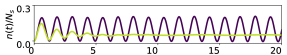
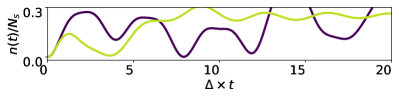
Figure 12: Evolution of photon population per each mode normalized by cluster size $N_{s}$, for $g/g_{c}=1.27$ and $(\theta_{0},\varphi_{0})=(0.7\pi,0)$. Top panel: the adiabatic limit $\omega_{c}/\Delta=5.0$ and for $\kappa=0$ (dark curve) and $\kappa/\Delta=0.5$ (light curve). Bottom panel: the same as top panel only for slow photons $\omega_{c}=\Delta$.

Eqs (132)-(134) describe the motion of classical angular momentum variables with a conserved vector length $\sqrt{\tilde{\sigma}\cdot\tilde{\sigma}}=1$. Adiabatic elimination of photons [180] amounts to approximate the integral in Eq. (134) as

$$\approx\expectationvalue{\sigma^{y}(t)}\expectationvalue{\sigma^{x}(t)}\int_{0}^{t}D^{\phi\phi}_{R}(t-t^{\prime})\,dt^{\prime}\approx\expectationvalue{\sigma^{y}(t)}\expectationvalue{\sigma^{x}(t)}\\ \times\int_{0}^{\infty}D^{\phi\phi}_{R}(t^{\prime})\,dt^{\prime}\approx-\frac{1}{\omega_{c}(\omega_{c}^{2}+\kappa^{2})}\expectationvalue{\sigma^{y}(t)}\expectationvalue{\sigma^{x}(t)}.$$ (136)

Substituting (136) into Eqs. (133) and (134) results in the MF equations of motion for LMG model with a coupling modified by photon loss according to $J\to J\omega_{c}^{2}/(\omega_{c}^{2}+\kappa^{2})$. From a physical point of view, the above derivation shows that at LO, our approximation maps each cluster to a classical LMG system without coupling to other clusters. Therefore, the LO approximation describes the FM to PM transition of an infinite range Ising model with retarded interactions. The critical coupling of this system is determined according to the condition $\Delta=J$ [116] to be

$$g_{c}=\frac{1}{2}\sqrt{\frac{\Delta(\omega_{c}^{2}+\kappa^{2})}{\omega_{c}}\frac{N+M}{M}}.$$ (137)

Although only valid in the adiabatic regime of the MF solution, we will use $g_{c}$ throughout this paper and scale the coupling $g$ according to it when comparing our results for different values of $\Delta$, $\omega_{c}$ or $\kappa$. Clearly, dynamics at LO do not have any features unexplored in the past, and we only report the results of our simulations as a consistency check of our approach. In Fig. 11 we have shown the dynamics of spins initiated close to an equilibrium state of Eqs. (132)-(134) inside the FM phase. We see that for fast photons (top panel of Fig. 11), the system remains close to the minimum with oscillations which are smoothed by photon loss. For slow photons when adiabatic elimination does not work (bottom panel of Fig. 11), the fluctuations induced by photons’ dynamics relieve FM correlations and can create rare tunneling events. With photon loss, the destructive effect of slow photons on FM order is reduced due to the effective damping that slows down the spins towards the bottom of the nearby energy minimum.

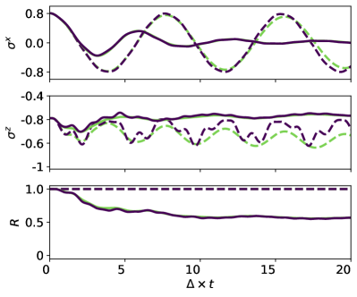
Figure 13: Comparison of spin dynamics at LO (dashed lines) and NLO (solid lines) approximations for a large spin size ($N_{s}=10^{5}$), following a PM quench ($g/g_{c}=0.71$) and in the limit of fast photons $\omega_{c}/\Delta=5$ with ($\kappa/\Delta=0.5$, light curves) and without (dark curves) photon loss. Top, middle and bottom rows show the evolution of $\expectationvalue{\sigma^{x}}$, $\expectationvalue{\sigma^{z}}$ and the expectation value of spin size, respectively. Spins dephase to a single point due to random static couplings in the system.

Having explored spin dynamics at LO, we now discuss the evolution of photon sector. As we said before, the response of photons given by the retarded function $D^{\phi\phi}_{R}$ is unaltered by interactions at LO. However, the symmetric correlation function of photons and photon population are affected by the coupling to spins. Spins pump cavity modes due to the presence of the transverse field $\Delta$, and as shown in Fig. 12, create large oscillations (if $\kappa=0$) or a superradiant burst (if $\kappa\neq 0$) in the population of photons $n(t)$. We do not discuss dynamics of the PM phase in LO approximation here due to their trivial nature, and will show them in comparison with NLO results later. The insufficiency of the LO approximation is clear by above observations. At this order of approximation, the size of each cluster $N_{s}$ only appears as an overall scaling factor in photon number $n(t)\propto N_{s}$, and spin dynamics do not depend on $N_{s}$. The latter is not physically valid, as we expect fluctuations to affect spin dynamics noticeably when the spin per each cluster $\hat{S}_{i}=\sum_{\lambda}\hat{\sigma}_{i\lambda}/2$ becomes smaller as $N_{s}$ is decreased. The other important shortcoming of LO approximation is visible in the dynamics of photon population in the adiabatic limit without loss, where the amplitude of the oscillations in $n(t)$ does not change and remains constant (Fig. 12). In reality, photons experience dissipation even in a perfect cavity, as they can be reabsorbed by spins over longer timescales and the system is expected to equilibrate eventually. It is clear from the discussion above that LO approximation fails to capture this effect. As we will see next, NLO corrections take into account fluctuations and the reabsorption of photons, in addition to non-trivial regimes of dynamics such as glassy behavior.

V.2 Results at NLO for Large Spins

Below we will report on the dynamics at NLO for quenches to PM and FM phases of the system, in the limit of large spin per cluster ($N_{s}=10^{5}$). We note that we label these phases according to the behavior of the system at the MF level. The dynamics may change significantly when going beyond MF theory, making these labels inaccurate a posteriori.

V.2.1 Dynamics in the paramagnetic phase

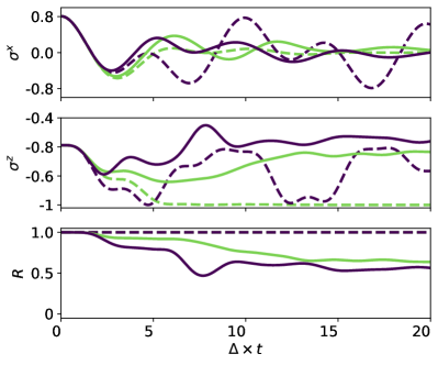
Figure 14: Comparison of spin dynamics at LO (dashed lines) and NLO (solid lines) approximations for a large spin size ($N_{s}=10^{5}$), following a PM quench ($g/g_{c}=0.71$) and in the limit of resonant photons $\omega_{c}=\Delta$ with ($\kappa/\Delta=0.5$, light curves) and without (dark curves) photon loss. Top, middle and bottom rows show the evolution of $\expectationvalue{\sigma^{x}}$, $\expectationvalue{\sigma^{z}}$ and the expectation value of spin size, respectively. Spins dephase to a single point due to random static couplings in the system.

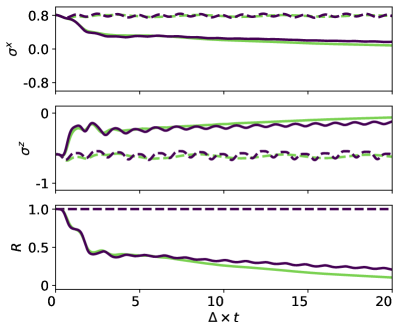
Figure 15: Comparison of spin dynamics at LO (dashed lines) and NLO (solid lines) approximations for a large spin size ($N_{s}=10^{5}$), following a FM quench ($g/g_{c}=1.27$) and in the limit of fast photons $\omega_{c}/\Delta=5$ with ($\kappa/\Delta=0.5$, light curves) and without (dark curves) photon loss. Top panel: following a quick collapse, the decay of FM order parameter strongly slows down and a prethermal plateau is formed. The middle and bottom panels show the evolution of $\expectationvalue{\sigma^{z}}$ and the radius of the Bloch sphere, respectively.

We initialize the system in the ground-state of photons and the spin state with $(\theta_{0},\varphi_{0})=(0.7\pi,0)$ in Eq. (131). We choose a coupling below $g_{c}$ given in Eq. (137), and consider both cases of perfect and lossy cavities. The results for fast photons ($\omega_{c}/\Delta=5$) are shown in Fig. (13), in comparison with LO results. We see that the evolution of $\expectationvalue{\sigma^{x}}$ is considerably altered by taking fluctuations into account. Spin dynamics is now damped even in the absence of photon loss. This is expected, as dissipation is a natural byproduct of interactions in a many-body system. We also see that photon loss has a minor impact on spin dynamics as it is weaker than the fluctuation-induced dissipation. As shown in the middle panel of Fig. 13, $\sigma^{z}$ shows a surprising behavior at NLO by not relaxing to its minimum value, in contrast to the LO result which at least, when $\kappa\neq 0$, approaches $-1$. However, there is a clear explanation for this phenomenon. The value of $g^{2}$ gives the variance of the disordered coupling in the system. This means that, while most of the individual couplings for each realization of the disorder are smaller than $g$, some of them are still large enough to weaken the PM configuration of the ground-state without causing a phase transition in the system. The fact that this behavior is purely due to random interactions is supported by our observation that the NLO approximation for non-disordered Dicke model results in the decay of spins into a state with $\sigma^{z}=-1$ in the PM phase. We also have shown the evolution of the spin vector size defined by

$$R(t)\equiv\sqrt{\expectationvalue{\sigma^{x}}^{2}+\expectationvalue{\sigma^{y}}^{2}+\expectationvalue{\sigma^{z}}^{2}},$$ (138)

in Fig. 13. While $R$ is a constant of motion of Eqs. (132)-(134), it changes when fluctuations are considered. The final state of the system is a PM with a smaller spin size. Note that $R(t\to\infty)$ is independent of the initial state and is always smaller than one even at the lowest temperatures, only due to the frustrated nature of the system. In the following discussion, $R(t)$ will be a useful proxy for assessing the impact of correlations in dynamics. It is the radius of the Bloch sphere, given at $t=0$ by the spin coherent state in Eq. (131), and a constant of motion for all-to-all interacting spin systems with homogeneous couplings and collective dissipation [119, 181, 19]. It stays constant over time because in this class of systems, the MF approximation is exact in the thermodynamic limit and therefore no higher order cumulants are formed, which would make $R(t)$ shrink, signaling the onset of a strongly correlated regime. Spin dynamics at NLO approximation for the case of resonant photons $\omega_{c}=\Delta$ are illustrated in Fig. 14. As expected, dynamics become more irregular both at LO and NLO and photon loss has a more dramatic effect on the dynamics.

V.2.2 Dynamics in the ferromagnetic phase

Figure 16: Evolution of spin vectors projected to the $x\hat{O}z$ plane for large cluster size $N_{s}=10^{5}$, in the adiabatic limit $\omega_{c}/\Delta=5$ (top panel) and resonant $\omega_{c}=\Delta$ (bottom panel) limits, for $\kappa/\Delta=0$ (dark curves) and $\kappa/\Delta=0.5$ (light curves). In the adiabatic limit, spins feature a spiral relaxation around the axis of FM ordering (dashed line) and towards the origin (parallel to the arrow).

We quench the coupling to $g=1.27g_{c}$ where a FM state is realized at LO as shown previously,. The initial spin vector is again taken to be $(\theta_{0},\varphi_{0})=(0.7\pi,0)$, such that spins are close to the ground-state of the classical model in Eqs. (132)-(134) at the chosen coupling strength. Similar to the PM case, we take a large spin size ($N_{s}=10^{5}$) where the effect of NLO corrections is supposed to be small. It will become clear that this is an incorrect assumption and NLO contributions are significant. The results of the numerics for the adiabatic limit $\omega_{c}/\Delta=5$ are depicted in Fig. 15 at LO and NLO approximations. At LO, $\sigma^{x}$ and $\sigma^{z}$ show small oscillations around the equilibrium of the MF dynamics and the spin vector is confined to the surface of the Bloch sphere ($R=1$). Fluctuations captured at NLO drastically alter the dynamics. All components of spin decay and the spin vector shrinks toward the center of the Bloch sphere. The spin decay features an interesting profile. For an initial period, the relaxation is quick and spins experience a collapse to a smaller but finite value. Following this, the relaxation becomes very slow and the spin vector spirals around the axis of FM order of the LO solution (Fig. 16). This situation is similar to the phenomenon of prethermalization in the quench dynamics of many-body quantum systems [67, 24, 79, 182, 183, 184, 185, 186, 187, 188, 189], although here the system can be open. The prethermal behavior is also seen in the time evolution of photon number $n(t)$ shown in Fig. 17a. During the prethermal plateau of spins, $n(t)$ has a nearly stationary value with a slow growth (visible in the overall slope of the light curve in Fig. 17b) towards the true equilibrium state. Photon losses only qualitatively affect spin dynamics, by weakly accelerating the process of relaxation.

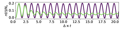
(a)

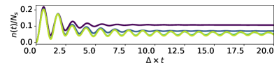
(b)

Figure 17: (a) Photon population for a quench into the ordered phase with $g/g_{c}=1.27$, $\omega_{c}/\Delta=5$ and $\kappa=0$ at LO (dark curve) and NLO (light curve). (b) Photon number per mode for $g/g_{c}=1.27$ and for $N=1000,\,200,\,20,\,5$ (light to dark curves). Relaxation of late-time oscillations is faster for smaller $N_{s}$.

Spin dynamics in the regime of resonant photons ($\omega_{c}=\Delta$) is shown in Fig. 18. We see that the relaxation is faster in this regime compared to the adiabatic regime as expected, since photon radiation is kinematically more favorable in this limit. Also, the prethermal plateau does not appear any longer due to the enhancement of relaxation. The spiral evolution of spin vector changes to an irregular form (right panel in Fig. 16), but still approaches the origin at long times.
As we emphasized before, labeling the system as a FM for $g>g_{c}$ is only valid at the MF level. It is clear from the previous section that the system is not truly a FM as the magnetization decays with time. In the upcoming sections, we will provide evidence that the system is, in fact, a spin glass (SG) in this regime. However, it is not possible to uniquely determine a SG by only looking at single spin observables. The only indirect evidence for SG that we have so far is the slow relaxation of magnetization. We again remark that our results are expected to be correct for $\eta\gtrsim 1$ where the model in Eq. (1) is expected to host a SG [96, 123].

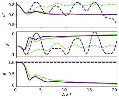
Figure 18: Spin dynamics at LO (dashed lines) and NLO (solid lines) approximations for $N_{s}=10^{5}$, following a FM quench ($g/g_{c}=1.27$) and in the limit of dynamically active photons $\omega_{c}=\Delta$ with ($\kappa/\Delta=0.5$, light curves) and without (dark curves) photon loss.

V.2.3 Dependence of the spin dynamics on cluster size

The number of spins per cluster $N_{s}$ is not only a control parameter for the expansion of the effective action, but it also determines the strength of fluctuations in the system. This assumption stems from the conventional understanding that larger spins often exhibit a more classical behavior compared to small spins [24]. Here, the size of the spin for each cluster is determined by the number of spins inside each cluster $N_{s}$. Our solution of the problem also supports the presence of stronger fluctuations for smaller values of spins per cluster. This can be seen, for example, in Eq. (121) where the fermion self-energy scales as $N_{s}^{-1}$. The dynamics of spins at NLO are shown in fig. 19 for different cluster sizes. The main effect of lowering $N_{s}$ or equivalently, increasing fluctuations is a faster relaxation of spins. As $N_{s}$ is decreased, the transient FM state lasts shorter. For sufficiently small $N_{s}$, the prethermal state is completely bypassed and the system experiences a quick relaxation towards equilibrium (Fig. 20). Similarly, photon number relaxes faster for smaller $N_{s}$, while for larger cluster sizes it has weakly damped oscillations (Fig. 17b).

V.3 Dynamics of spin glass

The results of NLO approximation given in previous sections indicate that the strong coupling limit of the model in Eq. (1) is not a FM and corrections due to frustration and fluctuations drastically change the MF phase diagram. From the $N_{s}=1$ limit of the problem [123, 96, 97], we know that the system hosts a SG at sufficiently low temperatures and strong couplings. The main questions are the following: (i) What are the physical signatures of SG in and out of equilibrium? (ii) Can our formalism capture the far from equilibrium dynamics of SG? (iii) How does the SG phase behave for different atomic ensemble sizes? In the upcoming sections, we will discuss two direct measures of SG phase. First, we consider the disorder average of the square of local magnetization of each spin ensemble which gives a proxy of the presence of frozen spin configurations. The second one is related to the ability of the system to retain its memory of the far past and is connected to the phenomenon of aging, encoded in 2-point correlation functions of the system for large time separations. We will demonstrate that 2PI can access both of these measures and is able to track their evolution in real time. At the end, we will discuss how the value of $N_{s}$ affects the SG phase.

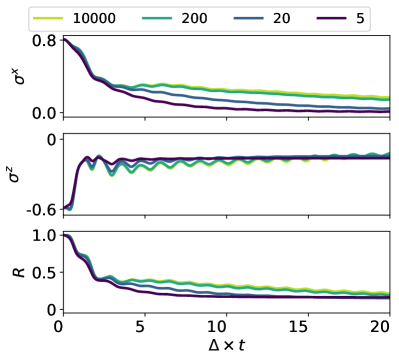
Figure 19: Spin dynamics for different numbers of cluster sizes $N_{s}$, following a FM quench ($g/g_{c}=1.27$) and in the limit of fast photons $\omega_{c}/\Delta=5$ without losses. Relaxation is faster for smaller cluster sizes due to enhanced fluctuations. The prethermal FM state disappears sooner as $N_{s}$ is decreased.

V.3.1 Characteristics of spin glass

According to Landau’s theory of phase transitions (PT), different phases of matter can be classified according to their symmetries [190, 170, 191]. A phase transition corresponds to a change in the symmetry group of a physical system. For example, the PM to FM transition of an Ising FM corresponds to the spontaneous breaking of the $Z_{2}$ symmetry of the Hamiltonian. The occurrence of the PT is signaled by the continuous growth of a parameter which vanishes on one side of the transition. Such parameter is termed as the order parameter and the way it grows with the control parameter of the transition provides us with important information about the nature of the PT [191, 170, 11]. While the PM to SG phase transition fits into the symmetry breaking paradigm, the proper definition of an order parameter for SG has been a subject of debate for decades, with various candidates [100, 94, 99]. In the following, we will consider two of these proposed order parameters to study the formation of SG in our system.

V.3.2 Local magnetization

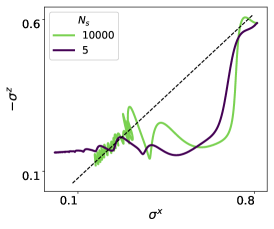
Figure 20: Comparison of spin vectors projected to the $xz$ plane for small and large cluster sizes, in adiabatic $\omega_{c}/\Delta=5$ and for $\kappa/\Delta=0$. The FM spiral of large spin ensembles crosses over to a quicker smooth relaxation for smaller values of $N_{s}$.

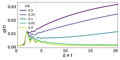
(a)

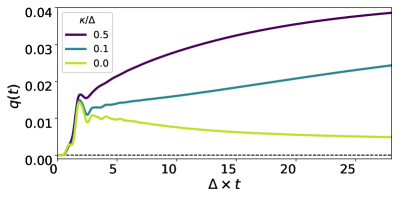
(b)

Figure 21: Formation of SG order for different values of system-bath coupling $\kappa$. (a) For $\theta_{0}=0.5\pi$, the energy density after the quench is large and the final temperature is too high to realize a SG, unless the system is allowed to cool down by coupling it to the bath. (b) For $\theta_{0}=0.7\pi$, energy density is smaller and the system enters a weak SG state without coupling to the bath, but it saturates to a smaller value of $q$, and hence, glass order is weaker in this case. The other parameters are $g/g_{c}=1.27$, $\omega_{c}/\Delta=5.0$, $N_{s}=5$ and $\eta=1$.

It is straightforward to define an order parameter for a FM. For instance, the quantum Ising model given by

$$H_{\mathrm{Ising}}=-\sum_{\expectationvalue{ij}}\sigma^{x}_{i}\sigma^{x}_{j}-g\sum_{i}\sigma^{z}_{i}-h\sum_{i}\sigma^{x}_{i},$$ (139)

is in FM phase if the thermal average $\expectationvalue{\sigma^{x}_{i}}$ is (i) finite and (ii) has the same sign for all $i$ if we take the thermodynamic limit and then, take $h\to 0$. One can also fix $h=0$ and start from an initial state with broken symmetry such that $\expectationvalue{\sigma^{x}}_{0}\neq 0$ and let the system evolve towards a FM equilibrium state. However, the symmetry will remain broken only in the thermodynamic limit. On the other hand, the PM phase is characterized by $\expectationvalue{\sigma^{x}_{i}}=0$ for all sites. At face value, a SG corresponds to a situation where the $Z_{2}$ symmetry of the Hamiltonian is broken such that $\expectationvalue{\sigma^{x}_{i}}$, but its value and sign are different for each site $i$, due to disordered interactions. In the thermodynamic limit, the average of $m_{i}\equiv\expectationvalue{\sigma_{i}^{x}}$ over all sites is zero

$$\lim_{N\to\infty}\frac{1}{N}\sum_{i}^{N}m_{i}=0.$$ (140)

Since the total magnetization is zero both in SG and PM phases, it cannot serve as an order parameter. However, we can define another quantity [100]

$$q=\lim_{N\to\infty}\frac{1}{N}\sum_{i}^{N}m_{i}^{2},$$ (141)

which is by definition finite for SG while still vanishing in the PM state. So far we assumed that we are working with a single realization of the disorder in the system. If we also average over the disorder, then Eq. (140) can be replaced with

$$\overline{m_{i}}=0,$$ (142)

while instead of (141) we can use

$$q=\overline{m_{i}^{2}}-\overline{m_{i}}^{2},$$ (143)

where following the notation of Section IV, the overline represents disorder averaging. We also have subtracted $\overline{m_{i}}^{2}$ which is vanishing at equilibrium, but can be finite when looking at non-equilibrium dynamics. We explained how to extract $q$ using the 2PI formalism in Sec. IV.8.3. In the following we will show the dynamics of $q(t)$ as the light-matter coupling $g$ and the photon loss $\kappa$ are varied.

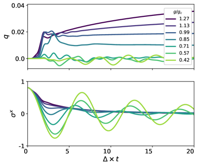
Figure 22: Dynamics of SG order parameter (top panel) and global magnetization (bottom panel) for different values of coupling strength. $g_{c}$ is the critical coupling in the MF theory. This plot shows that the observed value of $g_{c}$ is smaller than the one obtained at LO approximation. The other parameters are $\kappa/\Delta=0.5$, $\omega_{c}/\Delta=5.0$, $N_{s}=5$ and $\eta=1$.

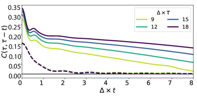
(a)

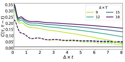
(b)

Figure 23: (a) Symmetric correlation function $C$ at different waiting times for quenches from an initial state with high energy density $\theta_{0}=\pi/2$. For $\kappa=0$ (dashed lines), the system heats up to PM state and $C$ quickly decays to zero for $t\to\infty$ (lines are almost on top of each other). For $\kappa/\Delta=0.5$ (solid lines) the system cools down to SG where $C$ remains finite for $t\to\infty$. (b) $C$ for an initial state with low energy density $\theta_{0}=0.7\pi$. Regardless of $\kappa$ the system ends up in the glass phase, however, SG order is stronger for $\kappa/\Delta=0.5$ (solid lines) where the system is cooled down, compared to $\kappa=0$ (dashed lines). For both figures $\omega_{c}/\Delta=5.0$, $g/g_{c}=1.27$, $\eta=1$ and $N_{s}=5$.

We initialize the system in a state with $\expectationvalue{\sigma^{x}_{i}}=1$ and quench $g$ from zero to a sufficiently large value. We monitor the dynamics of $q$ for different values of system-bath coupling from $\kappa=0$ (closed system) to $\kappa=0.5\Delta$. As can be seen in Fig. 21a, after some fluctuations caused by the quench, $q$ approaches zero at long times when the system is not coupled to the bath, while it grows to a finite value with a faster speed as $\kappa$ is increased. An explanation for this behavior is that the initial energy $E_{i}$ of the system with respect to the post-quench Hamiltonian is large enough to put the system in a high temperature equilibrium PM state if the system is closed. By coupling the system to the bath, we allow the system to lose its excessive energy by leaking the photons generated by the quench out of the cavity. Hence, the system cools down and enters the SG phase with finite $q$.

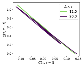
(a)

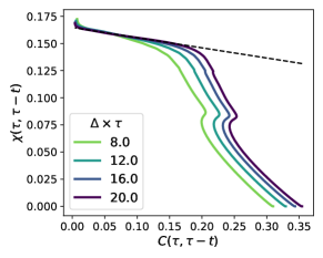
(b)

Figure 24: Integrated response $\chi$ versus $C$ for different waiting times $\tau$. (a) In PM phase, the slope is constant and is proportional to the inverse of temperature. (b) In SG state, dynamics have multiple time scales and the slope changes with $t$.

The explanation given above for the role of photon loss in the dynamics is supported by the behavior of quenches with smaller $E_{i}$. We note that $E_{i}$ can be calculated easily for the initial states considered in this work:

$$E_{i}=\frac{1}{2}NN_{s}\Delta\cos\theta_{0}.$$ (144)

since we have $g=0$ in the pre-quench hamiltonian. By initializing spins closer to $\theta_{0}=\pi$, we can reduce the energy density and attain a lower temperature final state for isolated quenches. For instance, for $\theta_{0}=0.7\pi$ the system enters the SG phase even without losses (Fig. 21b), although $q$ is smaller in this case due to the absence of cooling. We consider the effect of the coupling strength $g$ on glassy dynamics. Starting from $\theta_{0}=0.7\pi$ while connecting the system to an external bath by switching on the photon loss, we look at $q$ for quenches to different values of $g$ as shown in the top panel of Fig. 22. For weak couplings, we see that $q(t)$ approaches zero at long times, while showing small fluctuations at intermediate stages. We note that negative values for $q$ are not unphysical when $\expectationvalue{\sigma^{x}}$ is finite according to Eq. (143). When $g$ becomes large enough, $q$ saturates at a finite value at long times. We see in the bottom panel of Fig. 22 that spin dynamics changes from underdamped to overdamped at the same coupling where $q$ becomes finite. In Fig. 22 the coupling $g$ is scaled with $g_{c}$ which was the critical coupling of the MF limit in Eq. (137). A finite value of $q$ for $g/g_{c}<1$ indicates that NLO contributions shift the boundary of PM and SG phases towards SG.

V.3.3 Temporal correlations and aging phenomena

As discussed before, the diagnosis of SG phase requires the evidence of a frozen spin configuration which breaks the symmetry of the Hamiltonian and at the same time, has no global magnetization. In the previous section we discussed (the square of) the instantaneous magnetization for each site and showed that it is finite in the glass phase while magnetization relaxes to zero. The latter feature distinguished SG from FM. Another way to confirm a frozen spin state in the system is to look at the temporal correlation between the magnetization of each site at large time separations. For example, we take a cluster and its total spin operator $S^{x}$ at two different times $t$ and $t^{\prime}$. If spins are frozen, they do not fluctuate strongly in time and the overlap of magnetization for the same site at two different times is large. In fact, it remains finite even if $\absolutevalue{t-t^{\prime}}\to\infty$. For classical degrees of freedom one has

$$q_{\mathrm{EA}}\equiv\lim_{\absolutevalue{t-t^{\prime}}\to\infty}\overline{\expectationvalue{S^{x}(t)S^{x}(t^{\prime})}}>0,$$ (145)

which is the Edwards-Anderson (EA) order parameter [99, 100]. It is clear that the above condition can also imply FM order in the system. In order to exclude FM, the disorder averaged magnetization $\overline{\expectationvalue{S^{x}}}$ should also vanish. For the case of quantum operators in our problem, the correlator in Eq. (145) can be generalized to

$$C(\tau,\tau-t)\equiv\frac{1}{N_{s}^{2}}\sum_{\lambda,\lambda^{\prime}}^{N_{s}}\overline{\expectationvalue{\anticommutator{\sigma_{i\lambda}^{x}(\tau)}{\sigma_{i\lambda^{\prime}}^{x}(\tau-t)}}}_{c}.$$ (146)

We note that the off-diagonal elements $\lambda\neq\lambda^{\prime}$ in (146) can be non-zero. In the following, we consider the behavior of $C$ for the same quenches discussed in the previous section. It will be shown that $C$ changes its behavior at the same points where $q$ in Eq. (125) becomes finite. Therefore, both $C$ and $q$ are consistent measures of SG order in the system. We again look at the effect of photon loss on quenches from hot (with $\theta_{0}=0.5\pi$) and cold (with $\theta_{0}=0.7\pi$) initial states of the system, according to Eq. (144). We consider $C(\tau,\tau-t)$ for different values of the “waiting time” $\tau$ after the quench as a function of $t$. In Fig. 23a, we have shown $C$ for $\theta_{0}=\pi/2$ and for zero and finite $\kappa$. We see that $C$ behaves differently depending on whether the system is isolated or not. When the system is closed (dashed lines in Fig. 23a), it ends up in a high temperature PM state with correlations that relax quickly to equilibrium and show weak dependence on the waiting time after the quench $\tau$. The correlations also decay quickly with $t$, meaning that local magnetization loses the memory of its past quickly in the PM phase. When the system is allowed to cool down by emitting photons to the outside of the cavity, a SG phase emerges (solid lines in Fig. 23a). $C$ becomes strongly dependent on the waiting time $\tau$ and there is a crossover in the behavior of $C$ for $t\ll\tau$ and $t\approx\tau$. The latter behavior is termed aging [192, 193] and is another feature of quenches into SG phases. In aging, the decay of $C(\tau,\tau-t)$ with $t$ becomes slower for “older” systems with larger $\tau$. In this picture, there is a plateau in $C$ for $t\ll\tau$ (Fig. 23a) whose height gives the EA order parameter. The plateau is more visible in figures shown in upcoming sections.

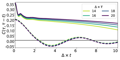
Figure 25: Dependence of $C$ on coupling strength for $g/g_{c}=1.27$ (solid lines) where aging and SG are realized, and for $g/g_{c}=0.57$ (dashed lines) with a PM profile. The other parameters are $\kappa/\Delta=0.5$, $\omega_{c}/\Delta=5.0$, $\theta_{0}=\pi$, $\eta=1$ and $N_{s}=5$.

Aging is closely related to the lack of thermalization in spin glasses [192, 194, 102, 195]. The system is unable to reach equilibrium because of its highly rugged energy landscape in which adjacent energy configurations, connected by local spin flips, are separated by large energy barriers. As a result, ergodicity is broken and system will not thermalize [194]. The relation between aging and thermalization can be made more explicit by using the fluctuation dissipation theorem (FDT) and fluctuation dissipation ratio (FDR) defined below. At thermal equilibrium, the symmetric correlation function $C(t,t^{\prime})$ and the response function $R(t,t^{\prime})$ of an observable $\mathcal{O}$ are connected to each other via FDT [101, 87, 11]:

$$R(t-t^{\prime})=-i\int\frac{d\omega}{2\pi}e^{-i\omega(t-t^{\prime})}\tanh(\frac{\omega}{2T})\tilde{C}(\omega),$$ (147)

where $\tilde{C}(\omega)=\int dt\exp(i\omega t)C(t)$ is the Fourier transform of $C$ and $T$ is the temperature. At long times or in the classical limit $\omega\ll T$, we can approximate $\tanh(\omega/2T)\approx\omega/2T$ to get for $t>t^{\prime}$

$$R(t,t^{\prime})\approx-\frac{1}{2T}\partial_{t^{\prime}}C(t,t^{\prime}).$$ (148)

By integration we get

$$C(t,t^{\prime})-C(t,t)=2T\chi(t,t^{\prime}),$$ (149)

where $\chi$ is the integrated response defined as

$$\chi(t,t^{\prime})\equiv\int_{t^{\prime}}^{t}R(t,t^{\prime\prime})\,dt^{\prime\prime}.$$ (150)

Eq. (149) can be generalized to out of equilibrium regimes as [196, 194, 197, 198]

$$C(\tau,\tau-t)-C(\tau,\tau)=2T_{\mathrm{eff}}(\tau,t)\chi(\tau,\tau-t),$$ (151)

where $T_{\mathrm{eff}}$ is the time-dependent effective temperature. $T_{\mathrm{eff}}$ can be read from the slope of the plot of $\chi$ versus $C$. If a system is coupled to an external bath with temperature $T$ the fluctuation dissipation ratio $X(\tau,t)$ is defined as

$$X(\tau,t)\equiv\frac{T}{T_{\mathrm{eff}}(\tau,t)}.$$ (152)

Therefore, $X$ measures the deviation of the system from true equilibrium at temperature $T$ [194, 195, 193]. For generic systems that thermalize efficiently, $T_{\mathrm{eff}}\to T$ and $X\to 1$. For glassy systems, on the other hand, $X$ can show a multistage behavior, where the plot of $\chi$ versus $C$ changes its slope. Furthermore, FDR may never reach the limit $X\to 1$, and the system will not thermalize at all.

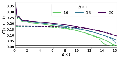
Figure 26: Dependence of $C$ on spin size $N_{s}$ for $N_{s}=5$ (solid lines) and $N_{s}=10^{3}$ (dashed lines) at different waiting times. We have taken $g/g_{c}=1.27$, $\kappa/\Delta=0.5$, $\omega_{c}/\Delta=5.0$ and $\eta=1$.

In Fig. 24a we have shown $\chi$ in terms of $C$ for the PM phase of our model. We see that the plots has an almost constant slope (small deviations are mostly due to the error of numerical integration in Eq. (150)) and therefore, the PM phase has a unique temperature. For quenches inside the SG phase (Fig. 24b), $\chi$ acquires a distinct profile. The long-time effective temperature (related to the slope of the dashed line in Fig. 24b) and the short-time effective temperature are different [102, 195, 199]. This is a a direct consequence of aging in the system. The EA order parameter can be read from the value of $C$ at which the change of slope happens. The effective temperature of SG in Fig. 24b) is larger than that of the PM in Fig. 24a by about a factor of $5$, and hence $X\approx 0.2$. We remark that there is a close connection between the violation of FDT and replica symmetry breaking (RSB) in spin glasses [102], which suggest that the model under consideration hosts RSB, in agreement with the recent cavity QED experiment of Ref. [93]. While photon loss was necessary to realize SG for the high energy initial state with $\theta_{0}=\pi/2$, if we reduce the initial energy density by starting from a lower energy state with $\theta_{0}=0.7\pi$, the system will becomes SG regardless of coupling it to the bath or not (Fig. 23b). However, the height of the plateau for $\kappa=0$ is smaller, as the quench inside the SG phase is shallower in this case. This is in complete agreement with the behavior of $q$ given in Figs. 21a and 21b. Using $C$, we have also confirmed the PM to SG transition as a function of $g$. As shown in Fig. 25, the system is a PM for $g/g_{c}=0.57$ even if it is cooled down by the bath and initiated in a low energy initial state with $\theta_{0}=\pi$, while it becomes a SG at a stronger coupling $g/g_{c}=1.27$. The evolution of $q$ for these two couplings was shown in Fig. 22, again in agreement with the profile of $C$.

V.3.4 Effect of spin size on spin glass formation

Thus far, we have answered questions (i) and (ii) posed at the beginning of Sec. V.3. In the following, we address (iii) by enquiring into the effect of spin size $N_{s}$ on the dynamical emergence of SG following the quench. We remark that up to this point, the results on SG were given for small spins $N_{s}=5$. We already discussed in Sec. V.2.3 how spin dynamics change as the number of spins per cluster is increased. We saw that for a symmetry broken initial state, FM correlations survive for long times after the quench for large $N_{s}$, while they relax quickly for small $N_{s}$. Below, we will investigate the explicit dependence of SG order on $N_{s}$. If we take the ground-state of free spins ($\theta_{0}=\pi$) as the initial state, glassiness shows a weak dependence on $N_{s}$. The behavior of $C$ for $N_{s}=5$ and $N_{s}=10^{3}$ is shown in Fig. 26. The main difference between small and large spins appears at $t\ll\tau$ where $C$ acquires a flat profile for $t\ll\tau$. Moreover, the EA order parameter is larger for smaller spin sizes. However, this dependence is weak if we consider the large difference between the two considered spin sizes in Fig. 26. The difference between the glassy dynamics of small and large spins is more pronounced if the initial state breaks the symmetry. $C$ is shown in Fig. 27 for the same waiting time but different initial states and spin sizes. Taking the height of the plateau in $C$ as a measure of SG order, in the regime of small spins, glassiness is not very sensitive to the initial magnetization of the system $\expectationvalue{\sigma^{x}}_{0}$, and SG order is only marginally stronger for $\theta_{0}=\pi$ compared to $\theta_{0}=\pi/2$. For large spins, the influence of initial magnetization on the dynamical formation of SG order is more pronounced and for larger values $\expectationvalue{\sigma^{x}}_{0}$, the relaxation of $q_{\mathrm{EA}}$ towards its final value becomes slower. An explanation for this behavior is that the prethermal FM order for large spins (Sec. V.2.3) acts as a competing order that temporarily suppresses the formation of SG order in the system.

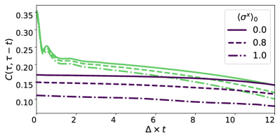
Figure 27: Dependence $C$ on the initial state before reaching the steady state for spin sizes $N_{s}=5$ (light curves) and $N_{s}=10^{3}$ (dark curves) at the same waiting time $\Delta\times T=20.0$ after the quench. We have taken $g/g_{c}=1.27$, $\kappa/\Delta=0.5$, $\omega_{c}/\Delta=5.0$ and $\eta=1$.

V.3.5 Spin glass formation away from adiabatic limit

At last, we consider the effect of changing photon frequency $\omega_{c}$ on the glass phase. 2PI formalism allows us to treat the problem in all ranges of frequencies and not just in the regime of fast photons where photons can be adiabatically eliminated [200, 180, 201]. We follow the same tradition as previous sections and scale $g$ with $g_{c}$ in Eq. (137). However, as will be explained later, this scaling does not alter the general picture given below. As explained before, initializing the system in a symmetric spin state helps it to reach the steady state earlier. This reduces the required numerical resources to access the SG phase in steady state (for a discussion of the numerical costs see Appendix C). We look at $C(\tau,\tau-t)$ for sufficiently large values of $\tau$ and a fixed $t$. This gives us an estimate of the EA order parameter $q_{\mathrm{EA}}$ as a measure of glassiness in the system. $q_{\mathrm{EA}}$ is shown in Fig. 28 for simulations with different photon frequencies. $q_{\mathrm{EA}}$ displays a peak below $\omega_{c}=\Delta$, vanishes quickly as $\omega_{c}\to 0$ and saturates in the adiabatic limit $\omega_{c}\gg\Delta$. The quick decay of SG order for small photon frequencies is an expected feature. For instance, phonons tend to relieve magnetic or density orderings in solid state platforms, as they have smaller energy gaps and are thermally excited easily. The observed peak in $q_{\mathrm{EA}}$ can be explained as a resonance effect by looking at the coherent part of the frequency-dependent interaction between spins following integrating out photons, which has the form

$$H_{\mathrm{int}}=\sum_{i,j}^{N}\sum_{\lambda,\lambda^{\prime}}^{N_{s}}\int\frac{d\omega}{2\pi}\sigma_{i\lambda}^{x}(-\omega)V^{ij}_{\mathrm{eff}}(\omega)\sigma_{j\lambda^{\prime}}^{x}(\omega),$$ (153)

with

$$V^{ij}_{\mathrm{eff}}(\omega)\sim\sum_{\alpha}^{M}g_{\alpha,i}g_{\alpha,j}\omega_{c}\real D^{R}(\omega).$$ (154)

$D^{R}$ is the bare retarded Green’s function of photons given by

$$D^{R}(\omega)=\frac{1}{(\omega+i\kappa)^{2}-\omega_{c}^{2}}.$$ (155)

Eq. (153) is obtained by integrating out photons in the original action, resulting in the following spin-spin interaction in the Keldysh action

$$S_{\sigma\sigma}=-\sum_{\alpha}^{M}\sum_{i,j}^{N}\sum_{\lambda,\lambda^{\prime}}^{N_{s}}g_{\alpha,i}g_{\alpha,j}\omega_{c}\int\frac{d\omega}{2\pi}\\ \begin{pmatrix}\sigma^{x}_{c}(-\omega)&\sigma^{x}_{q}(-\omega)\end{pmatrix}_{i\lambda}\begin{pmatrix}0&D^{A}(\omega)\\ D^{R}(\omega)&D^{K}(\omega)\end{pmatrix}\begin{pmatrix}\sigma^{x}_{c}(\omega)\\ \sigma^{x}_{q}(\omega)\end{pmatrix}_{j\lambda^{\prime}}.$$ (156)

We decompose the kernel matrix into its real and imaginary parts. The former is Hermitian and can be attributed to an effective Hamiltonian given by Eq. (153), while the imaginary part describes dissipation [88]. The $(c,q)$ indices in Eq. (156) are defined in Appendix B in terms of contour indices. To evaluate the strength of the interaction we can put $g_{\alpha,i}g_{\beta,j}\sim g^{2}$ to get

$$V_{\mathrm{eff}}(\omega)\sim g^{2}\omega_{c}\frac{\omega^{2}-\omega_{c}^{2}-\kappa^{2}}{(\omega^{2}-\omega_{c}^{2}-\kappa^{2})^{2}+4\kappa^{2}\omega^{2}}.$$ (157)

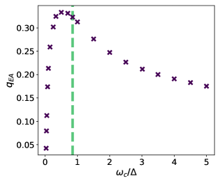
Figure 28: Dependence of SG order parameter at a fixed waiting time after the quench $\Delta\times\tau=12.0$ on photon frequency $\omega_{c}$. SG is strongest close to a resonance frequency near $\Delta$. Dashed line indicates the analytical estimate of the resonance frequency $\omega^{\star}$. The other parameters are $g/g_{c}=1.27$, $\kappa/\Delta=0.5$, $N_{s}=20$ and $\eta=1$.

In the adiabatic limit the relevant energy scales in the problem are small $\omega\ll\omega_{c},\kappa$ and we get

$$V_{\mathrm{eff}}(\omega\to 0)\sim-g^{2}\omega_{c}/(\omega_{c}^{2}+\kappa^{2})\sim-(\frac{g}{g_{c}})^{2}\Delta.$$ (158)

If we scale $g$ with $g_{c}$ such that $g^{2}=rg_{c}^{2}$ where $r$ is a dimensionless number, the effective interaction becomes insensitive to $\omega_{c}$. Therefore, changing $\omega_{c}$ should not affect SG order in the system. This is consistent with Fig. (28) where $q_{\mathrm{EA}}$ approaches a constant value at large frequencies. For smaller values of $\omega_{c}$ and $\kappa$, however, the dependence of effective interaction in Eq. (157) on $\omega$ becomes important. One possible approximation is to use the “on-shell approximation” and substitute $\omega\approx\Delta$. Using this approximation and expanding the effective spin-spin interaction to non-zero leading order in $\Delta$, recovers the atom-only description of Ref. [180] which also captures the dissipative part of the Lindblad dynamics. Nevertheless, this approach fails to describe the dependence of spin order on $\omega_{c}$, and in particular, the resonance behavior in Fig. 28. However, if we use the on-shell approximation and simply substitute $|\omega|=\Delta$ in $V_{\mathrm{eff}}(\omega)$ and do not expand it in $\Delta$, we find that $V_{\mathrm{eff}}$ has two peaks close to $\omega^{\star}$ given by

$$\omega^{\star}\equiv\sqrt{\Delta^{2}-\kappa^{2}},$$ (159)

with attractive ($V_{\mathrm{eff}}>0$) and repulsive ($V_{\mathrm{eff}}<0)$ sides for $\omega_{c}>\omega^{\star}$ and $\omega_{c}<\omega^{\star}$, respectively. $\omega^{\star}$ is marked in Fig. 28 and is in good agreement with the numerics. Nevertheless, there is a feature that cannot be straightforwardly explained by the on-shell approximation used above. $V_{\mathrm{eff}}(\Delta)$ vanishes at $\omega_{c}=\omega^{\star}$, but SG order does not show any signs of the suppression of interactions. A possible explanation for this discrepancy is that due to strong interactions, the spin spectral density defined in terms of the imaginary part of the response function (Eq. (118))

$$\mathcal{A}(\omega)=-\frac{(N+M)N_{s}}{4}\imaginary V^{22}(\omega),$$ (160)

is modified compared to the non-interacting limit and the atomic peak at $\omega=\Delta$ is highly broadened. It is believed that quantum SGs are critical with a gapless spectrum of excitations [199, 96, 202, 97]. For SK and disordered $SU(N)$ Heisenberg models, Refs. [202] and [199] obtained an Ohmic spectrum with $\sim\omega$. For closed Dicke SG at zero temperature, Ref. [96] predicted a similar Ohmic profile, while for Dicke SG connected to a Markovian bath Ref. [97] obtained a sub-Ohmic $\sim\omega^{\frac{1}{2}}$ dependence for $\omega\lesssim\kappa$. We have plotted the atomic spectral density for a low temperature quench without photon losses within our approach in Fig. 29. We see that $\mathcal{A}(\omega)$ displays a gapless spectrum at low frequencies, but with a sub-Ohmic dispersion $\sim\omega^{\frac{1}{2}}$, even though the system is not coupled to a Markovian bath. One explanation, although unlikely due to the similar symmetry of this model to the SK model, is that the system is in a different universality class with different exponents. Another possibility is that the final state long after the quench is at finite temperature with many emitted photons existing in the cavity, which act as an effective bath for spins. The exponent can be read experimentally using RF spectroscopy to compare with theoretical predictions.

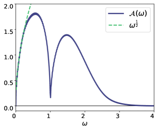
Figure 29: Atom spectral density in the glass phase for a long waiting time after the quench $\Delta\times\tau=60.0$ as function of frequency. Atoms form a continuum of sub-Ohmic modes at small energies. The minimum is due to vacuum Rabi splitting. The other parameters are $g/g_{c}=1.27$, $\kappa=0$, $\theta_{0}=\pi$, $N_{s}=5$ and $\eta=1$.

VI Conclusions

In this work we have provided a diagrammatic derivation of non-perturbative DE suited to describe spin glass formation far from equilibrium in the cavity QED platform of Refs. [37, 89, 90, 91]. Very recently, the same group has reported for the first time the observation of SG order [93] and associated replica symmetry breaking, which is a notoriously hard experimental task. We predict that SG order in this system can be obstructed by transient, competing ferromagnetism when the atomic ensembles trapped in the cavity are largely occupied. We show that SG order is enhanced by strong quantum fluctuations (few atoms per ensemble) and when photons are active and resonant with the atomic transitions. The set of DE derived here have the flexibility to explore simultaneously a broad set of parameters’ regimes (weak/strong coupling, variable ranges of $N_{s}$, adiabatic elimination and active photons) without resorting to descriptions valid only in a corner of parameter space. Our work sets also the stage for studying the crossover from strongly correlated regimes to semi-classical dynamics in other cavity QED platforms with tunable loading capabilities [36]. The dynamics of these systems are at reach of state-of-art 2PI-DE since interactions, although inhomogeneous, are all-to-all and this allows for more controlled diagrammatic expansions and numerical integration. At the same time, many of the new-generation cavity QED experiments combine short and all-to-all interactions, introducing a notion of dimensionality and lattice spacing that would make the numerical solution of the 2PI-DE more challenging.
We are currently making progress in this direction by exploring various experimental platforms:
Rydberg arrays integrated in optical cavities – The experiment in Ref. [35] marked the first combination of strong, short-range, Rydberg interactions with conventional photon-mediated long-range coupling. Analyzing these systems beyond mean-field theory opens up possibilities for exploring exotic phases of matter. These include spin liquids that are protected from dissipation [35] or limit cycles [203] that persist in the presence of strong classical and quantum noise. This line of research should also provide novel opportunities to explore topological order and lattice gauge theories in the context of atom-light interfaces [35].
Cavity QED with programable spin exchange interactions – Ref. [36] reports the realization of programmable non-local interactions in an array of atomic ensembles within an optical cavity. This experiment introduces a $U(1)$ variant [92] to the work discussed here, as it focuses on spin-exchange interactions rather than ferromagnetic ($Z_{2}$-invariant) ones. The ability to program the distance-dependent interactions with a sophisticated combination of Raman sidebands and magnetic field gradients enables the engineering of dimensionality, topology, and metric as needed. This opens the door to studying quantum optimization problems on tree-like [204] or fully connected geometries in cavity QED, bridging the gap between quantum information and many-body quantum optics.
Natural and synthetic correlated emission – In recent years, there has been a surge of interest in the study of dissipative spin problems that describe correlated emission in atomic ensembles. The key idea is that emission into free space involves multiple scattering and interference effects, making the phenomenon more complex than in traditional textbook quantum optics [205, 206, 207, 208, 209]. This mechanism is typically encoded in a Lindblad equation that is non-local in space, or equivalently non-diagonal in jump operators. While solutions for a few atomic excitations are accessible [208], the many-body regime of correlated emission remains largely unexplored. This would be of significance for Rydberg experiments realizing atomic mirrors via this mechanism [210, 211] and for applications in the cavity QED experiment of Ref. [36, 212], where correlated emission could be artificially engineered [213, 136, 44]. This would enable the synthesis of many-body entangled states using dissipation, by leveraging the full potent of programmable cavity QED in the domain of non-unitary dynamics.
On the interdisciplinary front, 2PI-DE for dissipative spin dynamics could also serve to guide dissipative quantum state preparation in hybrid AMO-spintronics platforms which rely on correlated emission to entangle NV centers [214].
This list of subjects is by no means exhaustive. For instance, 2PI-DE may be one of the few methods with sufficient versatility to treat the intrinsically strongly correlated dynamics of fermionic cavity QED experiments [38, 215, 216]. We hope that this set of potential applications will motivate readers from different communities to embark in the fascinating challenge to study the next generation of many-body quantum optics experiments using dynamical field theory methods.

VII Acknowledgements

We are thankful to A. N. Mikheev for carefully proof reading the manuscript, and to D. Gribben for early contributions to this project. HH and JM acknowledge financial support by the Deutsche Forschungsgemeinschaft (DFG, German Research Foundation): through Project-ID 429529648, TRR 306 QuCoLiMa (“Quantum Cooperativity of Light and Matter”) and through TRR 288 - 422213477 (project B09). This project has been supported by the QuantERA II Programme that has received funding from the European Union’s Horizon 2020 research and innovation programme under Grant Agreement No 101017733 (’QuSiED’) and by the DFG (project number 499037529). DC acknowledges support from the European Union, under European Research Council grant agreement No 101002107 (NEWSPIN); the Government of Spain under the Severo Ochoa Grant CEX2019-000910-S [MCIN/AEI/10.13039/501100011033]); QuantERA II project QuSiED, co-funded by the European Union Horizon 2020 research and innovation programme (No 101017733) and the Government of Spain (European Union NextGenerationEU/PRTR PCI2022-132945 funded by MCIN/AEI/10.13039/501100011033); Generalitat de Catalunya (CERCA program and AGAUR Project No. 2021 SGR 01442); Fundació Cellex, and Fundació Mir-Puig.

Appendix A Hubbard-Stratonovich transformation

We use the following identity

$$1=\int\mathcal{D}\quantity[\chi^{1},\chi^{2}]e^{iS_{\chi}},$$ (161)

where $S_{\chi}$ is defined in Eq. (69). This identity follows from the fact that the integral is Gaussian. Then, we shift the integration variable according to

$$\vec{\chi}_{\alpha i}\to\vec{\chi}_{\alpha i}+\hat{W}_{0}\otimes\vec{A}_{\alpha i}.$$ (162)

$\otimes$ is matrix multiplication over all indices (time and species). $\hat{W}_{0}$ was given by Eq. (71) and $\vec{A}_{\alpha i}$ is defined as

$$\vec{A}_{\alpha i}(t_{c})\equiv\begin{pmatrix}-\frac{2i}{\sqrt{N_{s}}}\sum_{\lambda}\psi^{y}_{i\lambda}(t_{c})\psi^{z}_{i\lambda}(t_{c})\\ \\ \sqrt{2\omega_{c}}g_{\alpha i}\phi_{\alpha}(t_{c})\end{pmatrix}.$$ (163)

Applying the shift yields

$$1=\int\mathcal{D}\quantity[\chi^{1},\chi^{2}]e^{iS_{\chi}+iS_{\chi\psi}+iS_{g\chi\phi}-iS_{\mathrm{int}}},$$ (164)

where $S_{\chi\psi}$, $S_{g\chi\phi}$ and $S_{\mathrm{int}}$ are respectively given by Eqs. (73), (74) and (66). Since $S_{\mathrm{int}}$ does not depend on $\chi$ we can move it to the LHS to get

$$e^{iS_{\mathrm{int}}}=\int\mathcal{D}\quantity[\chi^{1},\chi^{2}]e^{iS_{\chi}+iS_{\chi\psi}+iS_{g\chi\phi}}.$$ (165)

Therefore, we can substitute the RHS of the above expression in the original action.

Appendix B Dyson equations

For any practical calculation, we need to write equations in terms of normal time variables. DE are more transparent if we write fields in the classical/quantum basis defined as [101]

$$\phi_{c}(t) \equiv\frac{1}{\sqrt{2}}\quantity(\phi_{+}(t)+\phi_{-}(t)),$$ (166)

$$\phi_{q}(t) \equiv\frac{1}{\sqrt{2}}\quantity(\phi_{+}(t)-\phi_{-}(t)),$$ (167)

where $t$ is a normal time variable. The retarded, advanced and Keldysh (RAK) Green’s functions are defined as [101, 87]

$${G}^{R}(t,t^{\prime}) \equiv-i\expectationvalue{\phi_{c}(t)\phi_{q}(t^{\prime})},$$ (168)

$${G}^{A}(t,t^{\prime}) \equiv-i\expectationvalue{\phi_{q}(t)\phi_{c}(t^{\prime})},$$ (169)

$${G}^{K}(t,t^{\prime}) \equiv-i\expectationvalue{\phi_{c}(t)\phi_{c}(t^{\prime})}.$$ (170)

Accordingly, we define the 6-component fermion field

$$\Psi_{i\lambda}^{T}(t)\equiv\quantity(\psi^{x}_{c}(t),\psi^{y}_{c}(t),\psi^{z}_{c}(t),\psi^{x}_{q}(t),\psi^{y}_{q}(t),\psi^{z}_{q}(t)).$$ (171)

Where we have omitted the $i\lambda$ index on RHS for simplicity. Then, the action for free fermions $S_{\sigma}$ in Eq. (50) reads

$$S_{\sigma}=\frac{1}{2}\sum_{i}^{N}\sum_{\lambda}^{N_{s}}\int_{0}^{t}\Psi^{T}_{i\lambda}\hat{G}_{0}^{-1}\Psi_{i\lambda}\,dt,$$ (172)

with

$$\hat{G}_{0}^{-1} \equiv\begin{bmatrix}0&(\hat{G}_{0}^{A})^{-1}\\ (\hat{G}_{0}^{R})^{-1}&0\end{bmatrix},$$ (173)

$$(\hat{G}_{0}^{R})^{-1}=\quantity[(\hat{G}_{0}^{A})^{-1}]^{\dagger} \equiv\begin{bmatrix}i\partial_{t}&i\Delta&0\\ -i\Delta&i\partial_{t}&0\\ 0&0&i\partial_{t}\end{bmatrix}.$$ (174)

For self-energies we define

$$\hat{\Sigma}^{R} \equiv\frac{1}{2}\quantity(\hat{\Sigma}^{++}-\hat{\Sigma}^{+-}-\hat{\Sigma}^{--}+\hat{\Sigma}^{-+}),$$ (175)

$$\hat{\Sigma}^{A} \equiv\frac{1}{2}\quantity(\hat{\Sigma}^{++}+\hat{\Sigma}^{+-}-\hat{\Sigma}^{--}-\hat{\Sigma}^{-+}),$$ (176)

$$\hat{\Sigma}^{K} \equiv\frac{1}{2}\quantity(\hat{\Sigma}^{++}+\hat{\Sigma}^{+-}+\hat{\Sigma}^{--}+\hat{\Sigma}^{-+}).$$ (177)

DE have a simple structure in terms of RAK functions

$$\begin{bmatrix}0&(\hat{G}_{0}^{A})^{-1}-\hat{\Sigma}^{A}\\ (\hat{G}_{0}^{R})^{-1}-\hat{\Sigma}^{R}&-\hat{\Sigma}^{K}\end{bmatrix}\begin{bmatrix}\hat{G}^{K}&\hat{G}^{R}\\ \hat{G^{A}}&0\end{bmatrix}=\mathbb{1},$$ (178)

$$(\hat{G}_{0}^{R})^{-1}\hat{G}^{R}=\mathbb{1}+\hat{\Sigma}^{R}\hat{G}^{R},$$ (179)

$$(\hat{G}_{0}^{R})^{-1}\hat{G}^{K}=\hat{\Sigma}^{R}\hat{G}^{K}+\hat{\Sigma}^{K}\hat{G}^{A}.$$ (180)

The fermion self-energy matrix at NLO reads

$$\hat{\Sigma}_{\mathrm{NLO}}^{ss^{\prime}}=\begin{bmatrix}0&0&0\\ 0&\tilde{\Sigma}^{ss^{\prime}}_{yy}&\tilde{\Sigma}^{ss^{\prime}}_{yz}\\ 0&\tilde{\Sigma}^{ss^{\prime}}_{zy}&\tilde{\Sigma}^{ss^{\prime}}_{zz}\end{bmatrix},\quad(s,s^{\prime}=\pm).$$ (181)

Following Eq.(121), the expanded forms of the components of $\Sigma$ are given by

$$\tilde{\Sigma}^{ss^{\prime}}_{yy}(t,t^{\prime}) =+\frac{4i}{N_{s}}\quantity(MV^{11}_{ss^{\prime}}(t,t^{\prime})+M(M-1)U^{11}_{ss^{\prime}}(t,t^{\prime}))G_{zz}^{ss^{\prime}}(t,t^{\prime}),$$ (182)

$$\tilde{\Sigma}^{ss^{\prime}}_{zz}(t,t^{\prime}) =+\frac{4i}{N_{s}}\quantity(MV^{11}_{ss^{\prime}}(t,t^{\prime})+M(M-1)U^{11}_{ss^{\prime}}(t,t^{\prime}))G_{yy}^{ss^{\prime}}(t,t^{\prime}),$$ (183)

$$\tilde{\Sigma}^{ss^{\prime}}_{yz}(t,t^{\prime}) =-\frac{4i}{N_{s}}\quantity(MV^{11}_{ss^{\prime}}(t,t^{\prime})+M(M-1)U^{11}_{ss^{\prime}}(t,t^{\prime}))G_{zy}^{ss^{\prime}}(t,t^{\prime}),$$ (184)

$$\tilde{\Sigma}^{ss^{\prime}}_{zy}(t,t^{\prime}) =-\frac{4i}{N_{s}}\quantity(MV^{11}_{ss^{\prime}}(t,t^{\prime})+M(M-1)U^{11}_{ss^{\prime}}(t,t^{\prime}))G_{yz}^{ss^{\prime}}(t,t^{\prime}).$$ (185)

We do not write RAK self energies in terms of RAK Green’s functions as it is numerically less costly to find them from Eqs. (175)- (177). Defining $B_{x}(t)$ as

$$B_{x}(t)\equiv\frac{2M}{\sqrt{N_{s}}}\tilde{\chi}^{1}(t),$$ (186)

which captures the fermion self energy at LO (Eq. 116). Then, the expanded DE for retarded fermion Green’s functions are given by

$$i\partial_{t}G^{R}_{xx}(t,t^{\prime})+i\Delta G^{R}_{yx}(t,t^{\prime})=\delta(t-t^{\prime}),$$ (187)

$$i\partial_{t}G^{R}_{xy}(t,t^{\prime})+i\Delta G^{R}_{yy}(t,t^{\prime})=0,$$ (188)

$$i\partial_{t}G^{R}_{xz}(t,t^{\prime})+i\Delta G^{R}_{yz}(t,t^{\prime})=0,$$ (189)

$$i\partial_{t}G^{R}_{yx}(t,t^{\prime})-i\Delta G^{R}_{xx}(t,t^{\prime})-iB_{x}(t)G^{R}_{zx}(t,t^{\prime})=\int_{0}^{t}\quantity(\tilde{\Sigma}^{R}_{yy}(t,t^{\prime\prime})G^{R}_{yx}(t^{\prime\prime},t^{\prime})+\tilde{\Sigma}^{R}_{yz}(t,t^{\prime\prime})G^{R}_{zx}(t^{\prime\prime},t^{\prime}))\,dt^{\prime\prime},$$ (190)

$$i\partial_{t}G^{R}_{yy}(t,t^{\prime})-i\Delta G^{R}_{xy}(t,t^{\prime})-iB_{x}(t)G^{R}_{zy}(t,t^{\prime})=\delta(t-t^{\prime})+\int_{0}^{t}\quantity(\tilde{\Sigma}^{R}_{yy}(t,t^{\prime\prime})G^{R}_{yy}(t^{\prime\prime},t^{\prime})+\tilde{\Sigma}^{R}_{yz}(t,t^{\prime\prime})G^{R}_{zy}(t^{\prime\prime},t^{\prime}))\,dt^{\prime\prime},$$ (191)

$$i\partial_{t}G^{R}_{yz}(t,t^{\prime})-i\Delta G^{R}_{xz}(t,t^{\prime})-iB_{x}(t)G^{R}_{zz}(t,t^{\prime})=\int_{0}^{t}\quantity(\tilde{\Sigma}^{R}_{yy}(t,t^{\prime\prime})G^{R}_{yz}(t^{\prime\prime},t^{\prime})+\tilde{\Sigma}^{R}_{yz}(t,t^{\prime\prime})G^{R}_{zz}(t^{\prime\prime},t^{\prime}))\,dt^{\prime\prime},$$ (192)

$$i\partial_{t}G^{R}_{zx}(t,t^{\prime})+iB_{x}(t)G^{R}_{yx}(t,t^{\prime})=\int_{0}^{t}\quantity(\tilde{\Sigma}^{R}_{zy}(t,t^{\prime\prime})G^{R}_{yx}(t^{\prime\prime},t^{\prime})+\tilde{\Sigma}^{R}_{zz}(t,t^{\prime\prime})G^{R}_{zx}(t^{\prime\prime},t^{\prime}))\,dt^{\prime\prime},$$ (193)

$$i\partial_{t}G^{R}_{zy}(t,t^{\prime})+iB_{x}(t)G^{R}_{yy}(t,t^{\prime})=\int_{0}^{t}\quantity(\tilde{\Sigma}^{R}_{zy}(t,t^{\prime\prime})G^{R}_{yy}(t^{\prime\prime},t^{\prime})+\tilde{\Sigma}^{R}_{zz}(t,t^{\prime\prime})G^{R}_{zy}(t^{\prime\prime},t^{\prime}))\,dt^{\prime\prime},$$ (194)

$$i\partial_{t}G^{R}_{zz}(t,t^{\prime})+iB_{x}(t)G^{R}_{yz}(t,t^{\prime})=\delta(t-t^{\prime})+\int_{0}^{t}\quantity(\tilde{\Sigma}^{R}_{zy}(t,t^{\prime\prime})G^{R}_{yz}(t^{\prime\prime},t^{\prime})+\tilde{\Sigma}^{R}_{zz}(t,t^{\prime\prime})G^{R}_{zz}(t^{\prime\prime},t^{\prime}))\,dt^{\prime\prime}.$$ (195)

For Keldysh components we have

$$i\partial_{t}G^{K}_{xx}(t,t^{\prime})+i\Delta G^{K}_{yx}(t,t^{\prime}) =0,$$ (196)

$$i\partial_{t}G^{K}_{xy}(t,t^{\prime})+i\Delta G^{K}_{yy}(t,t^{\prime}) =0,$$ (197)

$$i\partial_{t}G^{K}_{xz}(t,t^{\prime})+i\Delta G^{K}_{yz}(t,t^{\prime}) =0,$$ (198)

$$i\partial_{t}G^{K}_{yx}(t,t^{\prime})-i\Delta G^{K}_{xx}(t,t^{\prime})-iB_{x}(t)G^{K}_{zx}(t,t^{\prime})=\int_{0}^{t}\Big{(}\tilde{\Sigma}^{R}_{yy}(t,t^{\prime\prime})G^{K}_{yx}(t^{\prime\prime},t^{\prime})+\tilde{\Sigma}^{R}_{yz}(t,t^{\prime\prime})G^{K}_{zx}(t^{\prime\prime},t^{\prime})\\ +\tilde{\Sigma}^{K}_{yy}(t,t^{\prime\prime})G^{A}_{yx}(t^{\prime\prime},t^{\prime})+\tilde{\Sigma}^{K}_{yz}(t,t^{\prime\prime})G^{A}_{zx}(t^{\prime\prime},t^{\prime})\Big{)}\,dt^{\prime\prime},$$ (199)

$$i\partial_{t}G^{K}_{yy}(t,t^{\prime})-i\Delta G^{K}_{xy}(t,t^{\prime})-iB_{x}(t)G^{K}_{zy}(t,t^{\prime})=\int_{0}^{t}\Big{(}\tilde{\Sigma}^{R}_{yy}(t,t^{\prime\prime})G^{K}_{yy}(t^{\prime\prime},t^{\prime})+\tilde{\Sigma}^{R}_{yz}(t,t^{\prime\prime})G^{K}_{zy}(t^{\prime\prime},t^{\prime})\\ +\tilde{\Sigma}^{K}_{yy}(t,t^{\prime\prime})G^{A}_{yy}(t^{\prime\prime},t^{\prime})+\tilde{\Sigma}^{K}_{yz}(t,t^{\prime\prime})G^{A}_{zy}(t^{\prime\prime},t^{\prime})\Big{)}\,dt^{\prime\prime},$$ (200)

$$i\partial_{t}G^{K}_{yz}(t,t^{\prime})-i\Delta G^{K}_{xz}(t,t^{\prime})-iB_{x}(t)G^{K}_{zz}(t,t^{\prime})=\int_{0}^{t}\Big{(}\tilde{\Sigma}^{R}_{yy}(t,t^{\prime\prime})G^{K}_{yz}(t^{\prime\prime},t^{\prime})+\tilde{\Sigma}^{R}_{yz}(t,t^{\prime\prime})G^{K}_{zz}(t^{\prime\prime},t^{\prime})\\ +\tilde{\Sigma}^{K}_{yy}(t,t^{\prime\prime})G^{A}_{yz}(t^{\prime\prime},t^{\prime})+\tilde{\Sigma}^{K}_{yz}(t,t^{\prime\prime})G^{A}_{zz}(t^{\prime\prime},t^{\prime})\Big{)}\,dt^{\prime\prime},$$ (201)

$$i\partial_{t}G^{K}_{zx}(t,t^{\prime})+iB_{x}(t)G^{K}_{yx}(t,t^{\prime})=\int_{0}^{t}\Big{(}\tilde{\Sigma}^{R}_{zy}(t,t^{\prime\prime})G^{K}_{yx}(t^{\prime\prime},t^{\prime})+\tilde{\Sigma}^{R}_{zz}(t,t^{\prime\prime})G^{K}_{zx}(t^{\prime\prime},t^{\prime})\\ +\tilde{\Sigma}^{K}_{zy}(t,t^{\prime\prime})G^{A}_{yx}(t^{\prime\prime},t^{\prime})+\tilde{\Sigma}^{K}_{zz}(t,t^{\prime\prime})G^{A}_{zx}(t^{\prime\prime},t^{\prime})\Big{)}\,dt^{\prime\prime},$$ (202)

$$i\partial_{t}G^{K}_{zy}(t,t^{\prime})+iB_{x}(t)G^{K}_{yy}(t,t^{\prime})=\int_{0}^{t}\Big{(}\tilde{\Sigma}^{R}_{zy}(t,t^{\prime\prime})G^{K}_{yy}(t^{\prime\prime},t^{\prime})+\tilde{\Sigma}^{R}_{zz}(t,t^{\prime\prime})G^{K}_{zy}(t^{\prime\prime},t^{\prime})\\ +\tilde{\Sigma}^{K}_{zy}(t,t^{\prime\prime})G^{A}_{yy}(t^{\prime\prime},t^{\prime})+\tilde{\Sigma}^{K}_{zz}(t,t^{\prime\prime})G^{A}_{zy}(t^{\prime\prime},t^{\prime})\Big{)}\,dt^{\prime\prime},$$ (203)

$$i\partial_{t}G^{K}_{zz}(t,t^{\prime})+iB_{x}(t)G^{K}_{yz}(t,t^{\prime})=\int_{0}^{t}\Big{(}\tilde{\Sigma}^{R}_{zy}(t,t^{\prime\prime})G^{K}_{yz}(t^{\prime\prime},t^{\prime})+\tilde{\Sigma}^{R}_{zz}(t,t^{\prime\prime})G^{K}_{zz}(t^{\prime\prime},t^{\prime})\\ +\tilde{\Sigma}^{K}_{zy}(t,t^{\prime\prime})G^{A}_{yz}(t^{\prime\prime},t^{\prime})+\tilde{\Sigma}^{K}_{zz}(t,t^{\prime\prime})G^{A}_{zz}(t^{\prime\prime},t^{\prime})\Big{)}\,dt^{\prime\prime}.$$ (204)

Advanced functions can be obtained from $\hat{G}^{A}=\quantity[\hat{G}^{R}]^{\dagger}$ and do not require separate computation. Photons fields in $(c,q)$ basis are cast into a multi-component field defined by

$$\Phi^{T}_{\alpha}(t)\equiv\quantity(\phi_{\alpha,c},\pi_{\alpha,c},\phi_{\alpha,q},\pi_{\alpha,q}),$$ (205)

with the free action (Eq. (58)

$$S_{\mathrm{ph}}=\frac{1}{2}\sum_{\alpha}^{M}\int_{0}^{t}\Phi_{\alpha}^{T}\hat{D}_{0}^{-1}\Phi_{\alpha}\,dt,$$ (206)

where

$$\hat{D}_{0}^{-1} \equiv\begin{bmatrix}0&(\hat{D}_{0}^{-1})^{A}\\ (\hat{D}_{0}^{-1})^{R}&(\hat{D}_{0}^{-1})^{K}\end{bmatrix},$$ (207)

$$(\hat{D}_{0}^{-1})^{R}=\quantity[(\hat{D}_{0}^{-1})^{A}]^{\dagger} \equiv\begin{bmatrix}-\omega_{c}^{2}&-\kappa-\partial_{t}\\ \kappa+\partial_{t}&-1\end{bmatrix},$$ (208)

$$(\hat{D}_{0}^{-1})^{K} \equiv\begin{bmatrix}2i\kappa\omega_{c}&0\\ 0&2i\kappa/\omega_{c}\end{bmatrix}.$$ (209)

Note that $(\hat{D}_{0}^{-1})^{K}$ is not the inverse of the bare Keldysh function, for details see Ref. [101]. Similar to fermions, DE has the general structure

$$\begin{bmatrix}0&(\hat{D}_{0}^{A})^{-1}-\hat{\Pi}^{A}\\ (\hat{D}_{0}^{R})^{-1}-\hat{\Pi}^{R}&(\hat{D}_{0}^{K})^{-1}-\hat{\Pi}^{K}\end{bmatrix}\begin{bmatrix}\hat{D}^{K}&\hat{D}^{R}\\ \hat{D^{A}}&0\end{bmatrix}=\mathbb{1},$$ (210)

$$(\hat{D}_{0}^{R})^{-1}\hat{D}^{R}=\mathbb{1}+\hat{\Pi}^{R}\hat{D}^{R},$$ (211)

$$(\hat{D}_{0}^{R})^{-1}\hat{D}^{K}+(\hat{D}_{0}^{K})^{-1}\hat{D}^{A}=\hat{\Pi}^{R}\hat{D}^{K}+\hat{\Pi}^{K}\hat{D}^{A}.$$ (212)

The photon self energy matrix $\hat{\Pi}$ only has one non-zero entry in $(\phi,\pi)$ basis

$$\hat{\Pi}^{R/A/K}=\begin{bmatrix}\Pi^{R/A/K}&&0\\ 0&&0\end{bmatrix},$$ (213)

where $\Pi$ was given in Eq. (122). The expanded DE for retarded photon functions are given by

$$-(\partial_{t}+\kappa)D^{R}_{\pi\phi}(t,t^{\prime})-\omega_{c}^{2}D^{R}_{\phi\phi}(t,t^{\prime})=\delta(t-t^{\prime})+\int_{0}^{t}\Pi^{R}(t,t^{\prime\prime})D^{R}_{\phi\phi}(t^{\prime\prime},t^{\prime})\,dt^{\prime\prime},$$ (214)

$$-(\partial_{t}+\kappa)D^{R}_{\pi\pi}(t,t^{\prime})-\omega_{c}^{2}D^{R}_{\phi\pi}(t,t^{\prime})=\int_{0}^{t}\Pi^{R}(t,t^{\prime\prime})D^{R}_{\phi\pi}(t^{\prime\prime},t^{\prime})\,dt^{\prime\prime},$$ (215)

$$+(\partial_{t}+\kappa)D^{R}_{\phi\phi}(t,t^{\prime})-D^{R}_{\pi\phi}(t,t^{\prime})=0,$$ (216)

$$+(\partial_{t}+\kappa)D^{R}_{\phi\pi}(t,t^{\prime})-D^{R}_{\pi\pi}(t,t^{\prime})=\delta(t-t^{\prime}),$$ (217)

and for Keldysh functions:

$$-(\partial_{t}+\kappa)D^{K}_{\pi\phi}(t,t^{\prime})-\omega_{c}^{2}D^{K}_{\phi\phi}(t,t^{\prime})+2i\kappa\omega_{c}D^{A}_{\phi\phi}(t,t^{\prime})=\int_{0}^{t}\quantity(\Pi^{R}(t,t^{\prime\prime})D^{K}_{\phi\phi}(t^{\prime\prime},t^{\prime})+\Pi^{K}(t,t^{\prime\prime})D^{A}_{\phi\phi}(t^{\prime\prime},t^{\prime}))\,dt^{\prime\prime},$$ (218)

$$-(\partial_{t}+\kappa)D^{K}_{\pi\pi}(t,t^{\prime})-\omega_{c}^{2}D^{K}_{\phi\pi}(t,t^{\prime})+2i\kappa\omega_{c}D^{A}_{\phi\pi}(t,t^{\prime})=\int_{0}^{t}\quantity(\Pi^{R}(t,t^{\prime\prime})D^{K}_{\phi\pi}(t^{\prime\prime},t^{\prime})+\Pi^{K}(t,t^{\prime\prime})D^{A}_{\phi\pi}(t^{\prime\prime},t^{\prime}))\,dt^{\prime\prime},$$ (219)

$$+(\partial_{t}+\kappa)D^{K}_{\phi\phi}(t,t^{\prime})-D^{K}_{\pi\phi}(t,t^{\prime})+\frac{2i\kappa}{\omega_{c}}D^{A}_{\pi\phi}(t,t^{\prime})=0,$$ (220)

$$+(\partial_{t}+\kappa)D^{K}_{\phi\pi}(t,t^{\prime})-D^{K}_{\pi\pi}(t,t^{\prime})+\frac{2i\kappa}{\omega_{c}}D^{A}_{\pi\pi}(t,t^{\prime})=0.$$ (221)

As mentioned in the main text, the off diagonal ($\alpha\neq\beta$) elements of Ising field Green’s functions have to be retained and DE for Ising field Green’s functions couple diagonal ($V$) and off diagonal ($U$) elements of $W$. The compact form of DE for $W$ is

$$\begin{bmatrix}0&(\hat{W}_{0}^{A})^{-1}-\hat{\Omega}^{A}\\ (\hat{W}_{0}^{R})^{-1}-\hat{\Omega}^{R}&-\hat{\Omega}^{K}\end{bmatrix}\begin{bmatrix}\hat{W}^{K}&\hat{W}^{R}\\ \hat{W}^{A}&0\end{bmatrix}=\mathbb{1}.$$ (222)

The self energy matrices are diagonal in the two dimensional space of the Ising field components

$$\hat{\Omega}^{R/A/K}=\begin{bmatrix}\Omega_{11}^{R/A/K}&0\\ 0&\Omega_{22}^{R/A/K}\end{bmatrix},$$ (223)

where $\Omega_{11}$ and $\Omega_{22}$ were given in Eqs. (123) and (124). It is convenient to decompose $W$ into its free and renormalized parts

$$W\equiv W_{0}+\tilde{W},$$ (224)

yielding

$$\tilde{W}^{R}=W_{0}^{R}\Omega^{R}W_{0}^{R}+W_{0}^{R}\Omega^{R}\tilde{W}^{R}.$$ (225)

$$\tilde{W}^{K}=W_{0}^{R}\Omega^{K}W_{0}^{A}+W_{0}^{R}\Omega^{R}\tilde{W}^{K}+W_{0}^{R}\Omega^{K}\tilde{W}^{A}.$$ (226)

The expanded form of Eq. (225) in the retarded sector is given by (note that $U_{0}=V^{11}_{0}=V^{22}_{0}=0$)

$$\tilde{V}^{R}_{11}(t,t^{\prime})=\frac{1}{N+M}\Omega_{22}^{R}(t,t^{\prime})+\frac{1}{\sqrt{N+M}}\int_{0}^{t}\Omega^{R}_{22}(t,t^{\prime\prime})\tilde{V}^{21}_{R}(t^{\prime\prime},t^{\prime})\,dt^{\prime\prime},$$ (227)

$$\tilde{U}^{R}_{11}(t,t^{\prime})=\frac{1}{\sqrt{N+M}}\int_{0}^{t}\Omega_{22}^{R}(t,t^{\prime\prime})\tilde{U}^{R}_{21}(t^{\prime\prime},t^{\prime})\,dt^{\prime\prime},$$ (228)

$$\tilde{V}^{R}_{12}(t,t^{\prime})=\tilde{U}^{R}_{12}(t,t^{\prime})=\frac{1}{\sqrt{N+M}}\int_{0}^{t}\Omega_{22}^{R}(t,t^{\prime\prime})\tilde{V}^{R}_{22}(t^{\prime\prime},t^{\prime})\,dt^{\prime\prime},$$ (229)

$$\tilde{V}^{R}_{21}(t,t^{\prime})=\tilde{U}^{R}_{21}(t,t^{\prime})=\frac{1}{\sqrt{N+M}}\int_{0}^{t}\Omega_{11}^{R}(t,t^{\prime\prime})\quantity(\tilde{V}^{R}_{11}(t^{\prime\prime},t^{\prime})+(M-1)\tilde{U}^{R}_{11}(t^{\prime\prime},t^{\prime}))\,dt^{\prime\prime},$$ (230)

$$\tilde{V}^{R}_{22}(t,t^{\prime})=\tilde{U}^{R}_{22}(t,t^{\prime})=\frac{1}{N+M}\Omega_{11}^{R}(t,t^{\prime})+\frac{1}{\sqrt{N+M}}\int_{0}^{t}\Omega_{11}^{R}(t,t^{\prime\prime})\quantity(\tilde{V}^{R}_{12}(t^{\prime\prime},t^{\prime})+(M-1)\tilde{U}^{R}_{12}(t^{\prime\prime},t^{\prime}))\,dt^{\prime\prime},$$ (231)

and for Eq. (226) we have

$$\tilde{V}^{K}_{11}(t,t^{\prime})=\frac{1}{N+M}\Omega_{22}^{K}(t,t^{\prime})+\frac{1}{\sqrt{N+M}}\int_{0}^{t}\quantity(\Omega^{R}_{22}(t,t^{\prime\prime})\tilde{V}_{21}^{R}(t^{\prime\prime},t^{\prime})+\Omega^{K}_{22}(t,t^{\prime\prime})\tilde{V}_{21}^{A}(t^{\prime\prime},t^{\prime}))\,dt^{\prime\prime},$$ (232)

$$\tilde{U}^{K}_{11}(t,t^{\prime})=\frac{1}{\sqrt{N+M}}\int_{0}^{t}\quantity(\Omega_{22}^{R}(t,t^{\prime\prime})\tilde{U}^{K}_{21}(t^{\prime\prime},t^{\prime})+\Omega_{22}^{K}(t,t^{\prime\prime})\tilde{U}^{A}_{21}(t^{\prime\prime},t^{\prime}))\,dt^{\prime\prime},$$ (233)

$$\tilde{V}^{K}_{12}(t,t^{\prime})=\tilde{U}^{K}_{12}(t,t^{\prime})=\frac{1}{\sqrt{N+M}}\int_{0}^{t}\quantity(\Omega_{22}^{R}(t,t^{\prime\prime})\tilde{V}^{K}_{22}(t^{\prime\prime},t^{\prime})+\Omega_{22}^{K}(t,t^{\prime\prime})\tilde{V}^{A}_{22}(t^{\prime\prime},t^{\prime}))\,dt^{\prime\prime},$$ (234)

$$\tilde{V}^{K}_{21}(t,t^{\prime})=\tilde{U}^{K}_{21}(t,t^{\prime})=\frac{1}{\sqrt{N+M}}\int_{0}^{t}\Omega_{11}^{R}(t,t^{\prime\prime})\quantity(\tilde{V}^{K}_{11}(t^{\prime\prime},t^{\prime})+(M-1)\tilde{U}^{K}_{11}(t^{\prime\prime},t^{\prime}))\,dt^{\prime\prime}\\ +\int_{0}^{t}\Omega_{11}^{K}(t,t^{\prime\prime})\quantity(\tilde{V}^{A}_{11}(t^{\prime\prime},t^{\prime})+(M-1)\tilde{U}^{A}_{11}(t^{\prime\prime},t^{\prime}))\,dt^{\prime\prime},$$ (235)

$$\tilde{V}^{K}_{22}(t,t^{\prime})=\tilde{U}^{K}_{22}(t,t^{\prime})=\frac{1}{N+M}\Omega_{11}^{K}(t,t^{\prime})+\frac{1}{\sqrt{N+M}}\int_{0}^{t}\Omega_{11}^{R}(t,t^{\prime\prime})\quantity(\tilde{V}^{K}_{12}(t^{\prime\prime},t^{\prime})+(M-1)\tilde{U}^{K}_{12}(t^{\prime\prime},t^{\prime}))\,dt^{\prime\prime}\\ +\int_{0}^{t}\Omega_{11}^{K}(t,t^{\prime\prime})\quantity(\tilde{V}^{A}_{12}(t^{\prime\prime},t^{\prime})+(M-1)\tilde{U}^{A}_{12}(t^{\prime\prime},t^{\prime}))\,dt^{\prime\prime}.$$ (236)

DE have a causal structure [143, 82, 145] with solutions that propagate in time such that the values of Green’s functions at each time step only depend on their values at previous times, allowing us to efficiently solve them using conventional numerical methods for differential equations.

Appendix C Numerical solution of Dyson equations

Solving Dyson equations (DE) is only possible using numerical integration. To solve DE numerically, we discretize both time variables of the correlation functions according to

$$G(t,t^{\prime})\to G(i,j)$$ (237)

and solve the problem on a two dimensional time grid with time spacing $\Delta t$. Assuming that correlation functions are known for $i,j\leq l$, which is an $l\times l$ square in the time grid, we evaluate the time derivates for fermion and photon Green’s functions using Dyson equations in Eqs. (187)-(204) and Eqs. (214)-(221) . The memory integrals only depend on the values of correlation functions at $i,j\leq l$ and can be evaluated using various numerical integration methods to be chosen depending on the desired accuracy. The equations for HS correlation functions in Eqs. (227)-(236) involve no time derivatives and HS correlation functions are directly found from their equations at each step. Using the values for the time derivatives allows us to predict the values of Green’s functions for $i,j\leq l+1$ using Euler’s method. However, the predicted value is usually not accurate enough and leads to numerical instabilities for long time evolutions. To remedy this issue, one can use more accurate approaches such as Runge-Kutta or predictor-corrector methods. For this work, we used a two-step predictor-corrector method. The reader is referred to an appendix in Ref. [82] for a detailed discussion of the two-step predictor-corrector method for DE. The main numerical costs are due to memory integrals on the RHS of DE. At each step of the integration, the numerical cost of evaluating memory integrals scales with $l^{2}$, where $l$ is the (discretized) evolution time since the initial state. The quadratic scaling with $l$ stems from the fact that at each step, memory integrals should be evaluated for $l$ points on the edge of the square given by $i,j\leq l$ and for each point, the cost of numerical integration scales with $l$. We can reduce the numerical costs by using the analytical properties of Green’s functions by only evaluating Green’s functions on one side of the diagonal ($i\geq j$) explicitly and finding their values for $i<j$ using a combination of complex conjugation or transposition. Nevertheless, the numerical costs increase with the evolution time. To reduce the cost further, one may truncate memory integrals and keep the memory of the system up to a certain point in the past. However, this truncation is not permissible for our glassy system since the integrands have significant contributions at long times due to strong memory effects in the SG phase, and omitting memory effects prevents us to capture glassy dynamics. In this case, the overall cost of evolving the system for $l$ steps using serial computation scales as $l^{3}$. Using parallel computation, we could achieve a slower increase of the runtime with $l$ given by

$$t_{\mathrm{runtime}}\sim l^{\beta},$$ (238)

where $2<\beta<3$.

Appendix D Evaluation of spin glass order parameter

After the procedure discussed in Section IV.8.3, fields of different replicas will be coupled to each other. Seemingly, this increases the complexity of the problem as one usually has to consider larger Green’s function matrices. However, the inter-replica couplings do not affect the dynamics of replica diagonal correlators. Therefore, the dynamics generated by DE given above are still valid. To evaluate replica off-diagonal Green’s functions, we have to derive extra dynamical equations that take replica diagonal Green’s functions as inputs. Further simplifications occur by noting that replica off diagonal fermion Green’s functions vanish due to the local $Z_{2}$ gauge symmetry of the fermionic representation for spins $\psi\to-\psi$. The only non-zero replica off diagonal self energies are

$$\underaccent{\sim}{\Pi}_{\mathrm{LO}}(t_{c},t^{\prime}_{c})=-2iNg^{2}\omega_{c}\tilde{\chi}^{2}(t_{c})\tilde{\chi}^{2}(t^{\prime}_{c}),$$ (239)

$$\underaccent{\sim}{\Pi}_{\mathrm{NLO}}(t_{c},t^{\prime}_{c})=2Ng^{2}\omega_{c}\underaccent{\sim}{V}^{22}(t_{c},t^{\prime}_{c}),$$ (240)

$$\underaccent{\sim}{\Omega}^{22}(t_{c},t^{\prime}_{c})=2g^{2}\omega_{c}\underaccent{\sim}{D}^{\phi\phi}(t_{c},t^{\prime}_{c}).$$ (241)

We also note that off diagonal Green’s functions only have Keldysh (symmetric) components. This is natural, as replicas are only mathematical entities without real physical interactions with each other. DE governing $\underaccent{\sim}{D}$ are given by

$$-(\partial_{t}+\kappa)\underaccent{\sim}{D}^{K}_{\phi\phi}(t,t^{\prime})+\underaccent{\sim}{D}^{K}_{\pi\phi}(t,t^{\prime})=0,$$ (242)

$$-(\partial_{t}+\kappa)\underaccent{\sim}{D}^{K}_{\pi\phi}(t,t^{\prime})-\omega_{c}^{2}\underaccent{\sim}{D}^{K}_{\phi\phi}(t,t^{\prime})=\\ \int_{0}^{t}\quantity(\Pi^{R}(t,t^{\prime\prime})\underaccent{\sim}{D}^{K}_{\phi\phi}(t^{\prime\prime},t^{\prime})+\underaccent{\sim}{\Pi}^{K}(t,t^{\prime\prime})D^{A}_{\phi\phi}(t^{\prime\prime},t^{\prime}))\,dt^{\prime\prime}.$$ (243)

For Ising field correlators we have

$$\underaccent{\sim}{V}^{K}_{22}(t,t^{\prime})=\frac{M}{\sqrt{N+M}}\int_{0}^{t}\Omega^{R}_{11}(t,t^{\prime\prime})\underaccent{\sim}{V}^{K}_{12}(t^{\prime\prime},t^{\prime})\,dt^{\prime\prime},$$ (244)

$$\underaccent{\sim}{V}^{K}_{12}(t,t^{\prime})=\frac{1}{\sqrt{N+M}}\int_{0}^{t}\Big{(}\Omega^{R}_{22}(t,t^{\prime\prime})\underaccent{\sim}{V}^{K}_{22}(t^{\prime\prime},t^{\prime})\\ +\underaccent{\sim}{\Omega}^{K}_{22}(t,t^{\prime\prime})V^{A}_{22}(t^{\prime\prime},t^{\prime})\Big{)}\,dt^{\prime\prime},$$ (245)

together with $\underaccent{\sim}{V}^{K}_{22}=\underaccent{\sim}{U}^{K}_{22}$ and $\underaccent{\sim}{V}^{K}_{12}=\underaccent{\sim}{U}^{K}_{12}$. These equations can be numerically solved using the same approach explained in Appendix C.

D.1 Equations of motion at LO

At LO fermion self energies will only have local terms captured by $B_{x}$ and the RHS of Eqs. (196)-(204) vanish. We want to find the time derivatives of spin expectation values. Using Eq.(49) we have

$$\derivative{t}\expectationvalue{\sigma^{\alpha}(t)}=-i\ \epsilon_{\alpha\beta\gamma}\derivative{t}\expectationvalue{\psi^{\beta}(t)\psi^{\gamma}(t)}\\ =\frac{1}{2}\epsilon_{\alpha\beta\gamma}\derivative{t}G^{K}_{\beta\gamma}(t,t).$$ (246)

We use the chain rule to write

$$\derivative{t}G^{K}_{\beta\gamma}(t,t)=\quantity(\partial_{t}+\partial_{t^{\prime}})G^{K}_{\beta\gamma}(t,t^{\prime})|_{t^{\prime}=t}.$$ (247)

In DE we have time derivatives of Green’s functions only with respect to $t$. However, $\partial_{t^{\prime}}G$ can be obtained easily by noting that

$$G^{K}_{\alpha\beta}(t,t^{\prime})=-G^{K}_{\beta\alpha}(t^{\prime},t),$$ (248)

$$\to\partial_{t^{\prime}}G^{K}_{\alpha\beta}(t,t^{\prime})|_{t=t^{\prime}}=-\partial_{t}G^{K}_{\beta\alpha}(t^{\prime},t)|_{t^{\prime}=t}.$$ (249)

For example, to find $\mathrm{d}\expectationvalue{\sigma^{z}}/\mathrm{d}t$ we use Eq.  (197)

$$\partial_{t}G^{K}_{xy}(t,t^{\prime})|_{t^{\prime}=t}=-\Delta G^{K}_{yy}(t,t),$$ (250)

and Eq. (199)

$$\partial_{t^{\prime}}G^{K}_{xy}(t,t^{\prime})|_{t^{\prime}=t}=-\partial_{t}G^{K}_{yx}(t^{\prime},t)|_{t^{\prime}=t}\\ =-\Delta G^{K}_{xx}(t,t)-B_{x}(t)G^{K}_{zx}(t,t),$$ (251)

to get

$$\derivative{t}G^{K}_{xy}(t,t)=-B_{x}(t)G^{K}_{zx}(t,t),$$ (252)

where we have used $G^{K}_{\alpha\alpha}(t,t)=0$. Using $G^{K}_{zx}(t,t)=\expectationvalue{\sigma^{y}(t)}$ we get

$$\derivative{t}\expectationvalue{\sigma^{z}(t)}=-B_{x}(t)\expectationvalue{\sigma^{y}(t)}.$$ (253)

Using $B_{x}$ from Eq.(119) we get

$$\derivative{t}\expectationvalue{\sigma^{z}(t)}=J\omega_{c}^{2}\int_{0}^{t}\expectationvalue{\sigma^{y}(t)}D^{\phi\phi}_{R}(t,t^{\prime})\expectationvalue{\sigma^{x}(t^{\prime})}\,dt^{\prime},$$ (254)

which is the LO equation of motion for $\expectationvalue{\sigma^{z}}$ given in Eq. (134). Eqs. (132) and (133) can be obtained similarly using DE at LO for other components of $G^{K}$.

Appendix E 2PI for the single mode Dicke model without disorder

For the Dicke model defined by

$$H=\frac{\Delta}{2}\sum_{i}^{N}\sigma^{z}_{i}+\omega_{c}a^{\dagger}a+\frac{g}{\sqrt{N}}\sum_{i}\quantity(a+a^{\dagger})\sigma^{x}_{i},$$ (255)

the Keldysh actions for spins and photons are the same as Eqs. (50) and (58) together with their RAK representations in Eqs. (172) and (206). The main difference is the spin-photon coupling part of the action

$$S_{\mathrm{int}}=2ig\sqrt{\frac{2\omega_{c}}{N}}\sum_{i}^{N}\oint dt_{c}\,\phi\psi^{y}_{i}\psi^{z}_{i}.$$ (256)

In this case, the expectation value of the photon field $\varphi\equiv\expectationvalue{\phi}$ can be finite. It is straightforward to show that at NLO, the 2PI action reads:

$$\Gamma\quantity[\varphi,\pi,D,G]=S_{\mathrm{cl}}[\varphi,\pi]+\frac{i}{2}\Tr\ln D^{-1}+\frac{i}{2}\Tr(D_{0}^{-1}D)\\ -\frac{i}{2}\Tr\ln G^{-1}-\frac{i}{2}\Tr(\tilde{G}_{0}^{-1}G)+\Gamma_{2}\quantity[D,G].$$ (257)

$S_{\mathrm{cl}}$ is obtained by substituting ${\varphi}$ and ${\pi}$ in $S_{\mathrm{ph}}$ in Eq. (58). $\tilde{G}_{0}$ contains the contribution of ${\varphi}$ to spin dynamics

$$\tilde{G}_{0}^{-1} \equiv\begin{bmatrix}0&(\tilde{G}_{0}^{A})^{-1}\\ (\tilde{G}_{0}^{R})^{-1}&0\end{bmatrix},$$ (258)

$$(\tilde{G}_{0}^{R})^{-1} \equiv\begin{bmatrix}i\partial_{t}&i\Delta&0\\ -i\Delta&i\partial_{t}&2ig\sqrt{2\omega_{c}/N}{\varphi}\\ 0&-2ig\sqrt{2\omega_{c}/N}{\varphi}&i\partial_{t}\end{bmatrix},$$ (259)

$$(\tilde{G}_{0}^{A})^{-1} =\quantity[(\tilde{G}_{0}^{R})^{-1}]^{\dagger}.$$ (260)

The last term $\Gamma_{2}$ is given at NLO ($\mathcal{O}(N^{0})$) by the diagram in Fig. 30 and reads as

$$\Gamma_{2}^{\mathrm{NLO}}=\frac{4\omega_{c}g^{2}}{N}\sum_{j}\oint\oint dt_{c}\,dt^{\prime}_{c}\,D^{\phi\phi}(t_{c},t^{\prime}_{c})\\ \times\big{(}G^{yy}_{jj}(t_{c},t^{\prime}_{c})G^{zz}_{jj}(t_{c},t^{\prime}_{c})-G^{yz}_{jj}(t_{c},t^{\prime}_{c})G^{zy}_{jj}(t_{c},t^{\prime}_{c})\big{)}.$$ (261)

Figure 30: The NLO contribution to 2PI action for the Dicke model.

DE for fermions are similar to those for the disordered model, provided that we substitute

$$B_{x}(t)=-2g\sqrt{\frac{2\omega_{c}}{N}}{\varphi}(t),$$ (262)

and use the following fermion self energies in the basis of contour branches

$$\Sigma^{ss^{\prime}}_{yz}(t,t^{\prime}) =-\frac{8i\omega_{c}g^{2}}{N}\,D^{ss^{\prime}}_{\phi\phi}(t,t^{\prime})G^{ss^{\prime}}_{zy}(t,t^{\prime}),$$ (263)

$$\Sigma^{ss^{\prime}}_{zy}(t,t^{\prime}) =-\frac{8i\omega_{c}g^{2}}{N}\,D^{ss^{\prime}}_{\phi\phi}(t,t^{\prime})G^{ss^{\prime}}_{yz}(t,t^{\prime}),$$ (264)

$$\Sigma^{ss^{\prime}}_{yy}(t,t^{\prime}) =+\frac{8i\omega_{c}g^{2}}{N}\,D^{ss^{\prime}}_{\phi\phi}(t,t^{\prime})G^{ss^{\prime}}_{zz}(t,t^{\prime}),$$ (265)

$$\Sigma^{ss^{\prime}}_{zz}(t,t^{\prime}) =+\frac{8i\omega_{c}g^{2}}{N}\,D^{ss^{\prime}}_{\phi\phi}(t,t^{\prime})G^{ss^{\prime}}_{yy}(t,t^{\prime}).$$ (266)

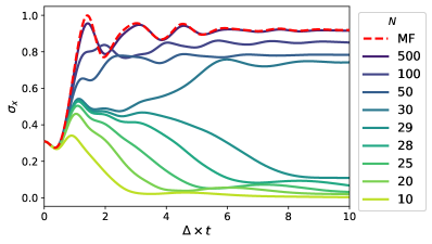
Figure 31: Spin dynamics for a quench into the SR phase of the Dicke model with photon loss, starting from $\theta_{0}=0.9\pi$. For $N<N^{\star}$ where $N^{\star}=30$, the symmetry is restored by fluctuations. $N^{\star}$ depends on the degree of symmetry breaking in the initial state. The other parameters are $g/g_{c}=1.6$, $\Delta/\omega_{c}=0.4$ and $\kappa/\omega_{c}=0.2$.

The equations of motion (EOM) for classical fields are given by

$$\quantity(\partial_{t}+\kappa){\varphi}={\pi},$$ (267)

$$\quantity(\partial_{t}+\kappa){\pi}+\omega_{0}^{2}{\varphi}+g\sqrt{2N\omega_{0}}G^{K}_{zy}(t,t)=0.$$ (268)

DE for photons are identical to those for the disordered system with the photon self energy

$$\Pi^{ss^{\prime}}(t,t^{\prime})=-8i\omega_{c}g^{2}\,\bigg{(}G^{ss^{\prime}}_{yz}(t,t^{\prime})G^{ss^{\prime}}_{zy}(t,t^{\prime})\\ -G^{ss^{\prime}}_{yy}(t,t^{\prime})G^{ss^{\prime}}_{zz}(t,t^{\prime})\bigg{)},$$ (269)

given in the basis of contour branches. Dynamics at LO are equivalent to the mean field treatment of the Dicke model with the critical coupling

$$g_{c}=\frac{1}{2}\sqrt{\frac{\Delta(\omega_{c}^{2}+\kappa^{2})}{\omega_{c}}}.$$ (270)

At NLO the inclusion of fluctuations modifies the dynamics for smaller system sizes. For instance, after quenching the coupling into the SR regime $g>g_{c}$, the system may not end up in a symmetry broken state with $\expectationvalue{a}\neq 0$, even if the initial state is not symmetric (Fig. 31). For smaller values of $N$, one should choose larger $\expectationvalue{\sigma^{x}}_{0}$, otherwise the symmetry will be restored. The symmetry restoration is due to the fact that for smaller values of $N$ fluctuation are stronger, resulting in the enhancement of the tunneling between the different minima in the energy of the system. This does not mean that the system is not in a SR state for small $N$. The photon population still saturates at a finite value $\sim N$.

References

- Browaeys and Lahaye [2020] A. Browaeys and T. Lahaye, Many-body physics with individually controlled rydberg atoms, Nature Physics 16, 132 (2020).
- Chang et al. [2014] D. E. Chang, V. Vuletić, and M. D. Lukin, Quantum nonlinear optics—photon by photon, Nature Photonics 8, 685 (2014).
- Byrnes et al. [2014] T. Byrnes, N. Y. Kim, and Y. Yamamoto, Exciton–polariton condensates, Nature Physics 10, 803 (2014).
- Monroe et al. [2021] C. Monroe, W. C. Campbell, L.-M. Duan, Z.-X. Gong, A. V. Gorshkov, P. W. Hess, R. Islam, K. Kim, N. M. Linke, G. Pagano, et al., Programmable quantum simulations of spin systems with trapped ions, Reviews of Modern Physics 93, 025001 (2021).
- Blais et al. [2021] A. Blais, A. L. Grimsmo, S. M. Girvin, and A. Wallraff, Circuit quantum electrodynamics, Reviews of Modern Physics 93, 025005 (2021).
- Altman [2021] E. Altman, Quantum simulators: Architectures and opportunities, PRX Quantum 2, 017003 (2021).
- Verstraete et al. [2009] F. Verstraete, M. M. Wolf, and J. Ignacio Cirac, Quantum computation and quantum-state engineering driven by dissipation, Nature physics 5, 633 (2009).
- Harrington et al. [2022] P. M. Harrington, E. J. Mueller, and K. W. Murch, Engineered dissipation for quantum information science, Nature Reviews Physics 4, 660 (2022).
- Diehl et al. [2008] S. Diehl, A. Micheli, A. Kantian, B. Kraus, H. Büchler, and P. Zoller, Quantum states and phases in driven open quantum systems with cold atoms, Nature Physics 4, 878 (2008).
- Sachdev [2023] S. Sachdev, Quantum Phases of Matter (Cambridge University Press, 2023).
- Altland and Simons [2010] A. Altland and B. D. Simons, Condensed matter field theory (Cambridge university press, 2010).
- Mahan [2000] G. D. Mahan, Many-particle physics (Springer Science & Business Media, 2000).
- Chaikin et al. [1995] P. M. Chaikin, T. C. Lubensky, and T. A. Witten, Principles of condensed matter physics, Vol. 10 (Cambridge university press Cambridge, 1995).
- Walther et al. [2006] H. Walther, B. T. Varcoe, B.-G. Englert, and T. Becker, Cavity quantum electrodynamics, Reports on Progress in Physics 69, 1325 (2006).
- Mivehvar et al. [2021] F. Mivehvar, F. Piazza, T. Donner, and H. Ritsch, Cavity qed with quantum gases: new paradigms in many-body physics, Advances in Physics 70, 1 (2021).
- Hosten et al. [2016a] O. Hosten, N. J. Engelsen, R. Krishnakumar, and M. A. Kasevich, Measurement noise 100 times lower than the quantum-projection limit using entangled atoms, Nature 529, 505 (2016a).
- Hosten et al. [2016b] O. Hosten, R. Krishnakumar, N. J. Engelsen, and M. A. Kasevich, Quantum phase magnification, Science 352, 1552 (2016b).
- Kelly et al. [2022] S. P. Kelly, J. K. Thompson, A. M. Rey, and J. Marino, Resonant light enhances phase coherence in a cavity qed simulator of fermionic superfluidity, Physical Review Research 4, L042032 (2022).
- Kirton et al. [2019] P. Kirton, M. M. Roses, J. Keeling, and E. G. Dalla Torre, Introduction to the dicke model: From equilibrium to nonequilibrium, and vice versa, Advanced Quantum Technologies 2, 1800043 (2019).
- Keeling et al. [2010] J. Keeling, M. Bhaseen, and B. Simons, Collective dynamics of bose-einstein condensates in optical cavities, Physical review letters 105, 043001 (2010).
- Valencia-Tortora et al. [2023] R. J. Valencia-Tortora, S. P. Kelly, T. Donner, G. Morigi, R. Fazio, and J. Marino, Crafting the dynamical structure of synchronization by harnessing bosonic multilevel cavity qed, Physical Review Research 5, 023112 (2023).
- Chelpanova et al. [2023] O. Chelpanova, A. Lerose, S. Zhang, I. Carusotto, Y. Tserkovnyak, and J. Marino, Intertwining of lasing and superradiance under spintronic pumping, Physical Review B 108, 104302 (2023).
- Kirton and Keeling [2017] P. Kirton and J. Keeling, Suppressing and restoring the dicke superradiance transition by dephasing and decay, Physical review letters 118, 123602 (2017).
- Marino et al. [2022] J. Marino, M. Eckstein, M. S. Foster, and A. M. Rey, Dynamical phase transitions in the collisionless pre-thermal states of isolated quantum systems: theory and experiments, Reports on Progress in Physics 85, 116001 (2022).
- Muniz et al. [2020] J. A. Muniz, D. Barberena, R. J. Lewis-Swan, D. J. Young, J. R. Cline, A. M. Rey, and J. K. Thompson, Exploring dynamical phase transitions with cold atoms in an optical cavity, Nature 580, 602 (2020).
- Lewis-Swan [2019] R. Lewis-Swan, Unifying scrambling, thermalization and entanglement through measurement of fidelity out-of-time-order correlators in the dicke model, Nature communications 10, 1581 (2019).
- Norcia et al. [2018] M. A. Norcia, R. J. Lewis-Swan, J. R. Cline, B. Zhu, A. M. Rey, and J. K. Thompson, Cavity-mediated collective spin-exchange interactions in a strontium superradiant laser, Science 361, 259 (2018).
- Dogra et al. [2019] N. Dogra, M. Landini, K. Kroeger, L. Hruby, T. Donner, and T. Esslinger, Dissipation-induced structural instability and chiral dynamics in a quantum gas, Science 366, 1496 (2019).
- Ferri et al. [2021] F. Ferri, R. Rosa-Medina, F. Finger, N. Dogra, M. Soriente, O. Zilberberg, T. Donner, and T. Esslinger, Emerging dissipative phases in a superradiant quantum gas with tunable decay, Physical Review X 11, 041046 (2021).
- Dreon et al. [2022] D. Dreon, A. Baumgärtner, X. Li, S. Hertlein, T. Esslinger, and T. Donner, Self-oscillating pump in a topological dissipative atom–cavity system, Nature 608, 494 (2022).
- Baumann et al. [2010] K. Baumann, C. Guerlin, F. Brennecke, and T. Esslinger, Dicke quantum phase transition with a superfluid gas in an optical cavity, nature 464, 1301 (2010).
- Kongkhambut et al. [2022] P. Kongkhambut, J. Skulte, L. Mathey, J. G. Cosme, A. Hemmerich, and H. Keßler, Observation of a continuous time crystal, Science 377, 670 (2022).
- Keßler et al. [2021] H. Keßler, P. Kongkhambut, C. Georges, L. Mathey, J. G. Cosme, and A. Hemmerich, Observation of a dissipative time crystal, Physical Review Letters 127, 043602 (2021).
- Klinder et al. [2015] J. Klinder, H. Keßler, M. Wolke, L. Mathey, and A. Hemmerich, Dynamical phase transition in the open dicke model, Proceedings of the National Academy of Sciences 112, 3290 (2015).
- Kong et al. [2021] H. Kong, J. Taylor, Y. Dong, and K. Choi, Melting a rydberg ice to a topological spin liquid with cavity vacuum fluctuation, arXiv preprint arXiv:2109.03741 (2021).
- Periwal et al. [2021] A. Periwal, E. S. Cooper, P. Kunkel, J. F. Wienand, E. J. Davis, and M. Schleier-Smith, Programmable interactions and emergent geometry in an array of atom clouds, Nature 600, 630 (2021).
- Kroeze et al. [2023a] R. M. Kroeze, B. P. Marsh, K.-Y. Lin, J. Keeling, and B. L. Lev, High cooperativity using a confocal-cavity–qed microscope, PRX Quantum 4, 020326 (2023a).
- Sauerwein et al. [2023] N. Sauerwein, F. Orsi, P. Uhrich, S. Bandyopadhyay, F. Mattiotti, T. Cantat-Moltrecht, G. Pupillo, P. Hauke, and J.-P. Brantut, Engineering random spin models with atoms in a high-finesse cavity, Nature Physics , 1 (2023).
- Bharti et al. [2022] K. Bharti, A. Cervera-Lierta, T. H. Kyaw, T. Haug, S. Alperin-Lea, A. Anand, M. Degroote, H. Heimonen, J. S. Kottmann, T. Menke, et al., Noisy intermediate-scale quantum algorithms, Reviews of Modern Physics 94, 015004 (2022).
- Sørensen and Mølmer [2002] A. S. Sørensen and K. Mølmer, Entangling atoms in bad cavities, Physical Review A 66, 022314 (2002).
- Rudelis [2023] A. Rudelis, A Cavity-Coupled Rydberg Atom Array Platform for Quantum Computing, Ph.D. thesis, Massachusetts Institute of Technology (2023).
- Chen et al. [2022] Y.-T. Chen, M. Szurek, B. Hu, J. de Hond, B. Braverman, and V. Vuletic, High finesse bow-tie cavity for strong atom-photon coupling in rydberg arrays, Optics Express 30, 37426 (2022).
- Marsh et al. [2021] B. P. Marsh, Y. Guo, R. M. Kroeze, S. Gopalakrishnan, S. Ganguli, J. Keeling, and B. L. Lev, Enhancing associative memory recall and storage capacity using confocal cavity qed, Phys. Rev. X 11, 021048 (2021).
- Seetharam et al. [2022a] K. Seetharam, A. Lerose, R. Fazio, and J. Marino, Correlation engineering via nonlocal dissipation, Phys. Rev. Res. 4, 013089 (2022a).
- Schachenmayer et al. [2015a] J. Schachenmayer, A. Pikovski, and A. M. Rey, Many-body quantum spin dynamics with monte carlo trajectories on a discrete phase space, Physical Review X 5, 011022 (2015a).
- Mink et al. [2022] C. D. Mink, D. Petrosyan, and M. Fleischhauer, Hybrid discrete-continuous truncated wigner approximation for driven, dissipative spin systems, Physical Review Research 4, 043136 (2022).
- Huber et al. [2022] J. Huber, A. M. Rey, and P. Rabl, Realistic simulations of spin squeezing and cooperative coupling effects in large ensembles of interacting two-level systems, Physical Review A 105, 013716 (2022).
- Huber et al. [2021] J. Huber, P. Kirton, and P. Rabl, Phase-space methods for simulating the dissipative many-body dynamics of collective spin systems, SciPost Physics 10, 045 (2021).
- Verstraelen et al. [2023] W. Verstraelen, D. Huybrechts, T. Roscilde, and M. Wouters, Quantum and classical correlations in open quantum spin lattices via truncated-cumulant trajectories, PRX Quantum 4, 030304 (2023).
- Kelly et al. [2021] S. P. Kelly, A. M. Rey, and J. Marino, Effect of active photons on dynamical frustration in cavity qed, Physical Review Letters 126, 133603 (2021).
- Mc Keever and Szymańska [2021] C. Mc Keever and M. Szymańska, Stable ipepo tensor-network algorithm for dynamics of two-dimensional open quantum lattice models, Physical Review X 11, 021035 (2021).
- Cui et al. [2015] J. Cui, J. I. Cirac, and M. C. Bañuls, Variational matrix product operators for the steady state of dissipative quantum systems, Physical review letters 114, 220601 (2015).
- Gangat et al. [2017] A. A. Gangat, I. Te, and Y.-J. Kao, Steady states of infinite-size dissipative quantum chains via imaginary time evolution, Physical review letters 119, 010501 (2017).
- Kilda et al. [2021] D. Kilda, A. Biella, M. Schirò, R. Fazio, and J. Keeling, On the stability of the infinite projected entangled pair operator ansatz for driven-dissipative 2d lattices, SciPost Physics Core 4, 005 (2021).
- Kshetrimayum et al. [2017] A. Kshetrimayum, H. Weimer, and R. Orús, A simple tensor network algorithm for two-dimensional steady states, Nature communications 8, 1 (2017).
- Mascarenhas et al. [2015] E. Mascarenhas, H. Flayac, and V. Savona, Matrix-product-operator approach to the nonequilibrium steady state of driven-dissipative quantum arrays, Physical Review A 92, 022116 (2015).
- Weimer et al. [2021] H. Weimer, A. Kshetrimayum, and R. Orús, Simulation methods for open quantum many-body systems, Reviews of Modern Physics 93, 015008 (2021).
- Kelly et al. [2020] S. P. Kelly, R. Nandkishore, and J. Marino, Exploring many-body localization in quantum systems coupled to an environment via wegner-wilson flows, Nuclear Physics B 951, 114886 (2020).
- Jin et al. [2016] J. Jin, A. Biella, O. Viyuela, L. Mazza, J. Keeling, R. Fazio, and D. Rossini, Cluster mean-field approach to the steady-state phase diagram of dissipative spin systems, Phys. Rev. X 6, 031011 (2016).
- Zhu et al. [2019] B. Zhu, J. Marino, N. Y. Yao, M. D. Lukin, and E. A. Demler, Dicke time crystals in driven-dissipative quantum many-body systems, New Journal of Physics 21, 073028 (2019).
- Berges [2002] J. Berges, Controlled nonperturbative dynamics of quantum fields out of equilibrium, Nuclear Physics A 699, 847 (2002).
- Berges [2004] J. Berges, Introduction to nonequilibrium quantum field theory, in AIP Conference Proceedings, Vol. 739 (American Institute of Physics, 2004) pp. 3–62.
- Cornwall et al. [1974] J. M. Cornwall, R. Jackiw, and E. Tomboulis, Effective action for composite operators, Phys. Rev. D 10, 2428 (1974).
- Aarts et al. [2002] G. Aarts, D. Ahrensmeier, R. Baier, J. Berges, and J. Serreau, Far-from-equilibrium dynamics with broken symmetries from the expansion of the 2pi effective action, Phys. Rev. D 66, 045008 (2002).
- Cooper et al. [2003] F. Cooper, J. F. Dawson, and B. Mihaila, Quantum dynamics of phase transitions in broken symmetry field theory, Phys. Rev. D 67, 056003 (2003).
- Arrizabalaga et al. [2004a] A. Arrizabalaga, J. Smit, and A. Tranberg, Tachyonic preheating using 2pi-1/n dynamics and the classical approximation, Journal of High Energy Physics 2004, 017 (2004a).
- Berges et al. [2004] J. Berges, S. Borsányi, and C. Wetterich, Prethermalization, Phys. Rev. Lett. 93, 142002 (2004).
- Berges et al. [2011] J. Berges, D. Gelfand, and J. Pruschke, Quantum theory of fermion production after inflation, Phys. Rev. Lett. 107, 061301 (2011).
- Berges and Roth [2011] J. Berges and S. Roth, Topological defect formation from 2pi effective action techniques, Nuclear Physics B 847, 197 (2011).
- Gasenzer et al. [2014] T. Gasenzer, L. McLerran, J. M. Pawlowski, and D. Sexty, Gauge turbulence, topological defect dynamics, and condensation in higgs models, Nuclear Physics A 930, 163 (2014).
- Nowak et al. [2014] B. Nowak, J. Schole, and T. Gasenzer, Universal dynamics on the way to thermalization, New Journal of Physics 16, 093052 (2014).
- Piñeiro Orioli et al. [2015] A. Piñeiro Orioli, K. Boguslavski, and J. Berges, Universal self-similar dynamics of relativistic and nonrelativistic field theories near nonthermal fixed points, Phys. Rev. D 92, 025041 (2015).
- Berges et al. [2017] J. Berges, K. Boguslavski, A. Chatrchyan, and J. Jaeckel, Attractive versus repulsive interactions in the bose-einstein condensation dynamics of relativistic field theories, Phys. Rev. D 96, 076020 (2017).
- Berges and Wallisch [2017] J. Berges and B. Wallisch, Nonthermal fixed points in quantum field theory beyond the weak-coupling limit, Phys. Rev. D 95, 036016 (2017).
- Walz et al. [2018] R. Walz, K. Boguslavski, and J. Berges, Large- kinetic theory for highly occupied systems, Phys. Rev. D 97, 116011 (2018).
- Rey et al. [2004] A. M. Rey, B. L. Hu, E. Calzetta, A. Roura, and C. W. Clark, Nonequilibrium dynamics of optical-lattice-loaded bose-einstein-condensate atoms: Beyond the hartree-fock-bogoliubov approximation, Phys. Rev. A 69, 033610 (2004).
- Balzer and Bonitz [2009] K. Balzer and M. Bonitz, Nonequilibrium properties of strongly correlated artificial atoms—a green’s functions approach, Journal of Physics A: Mathematical and Theoretical 42, 214020 (2009).
- Kronenwett and Gasenzer [2011] M. Kronenwett and T. Gasenzer, Far-from-equilibrium dynamics of an ultracold fermi gas, Applied Physics B 102, 469 (2011).
- Babadi et al. [2015] M. Babadi, E. Demler, and M. Knap, Far-from-equilibrium field theory of many-body quantum spin systems: Prethermalization and relaxation of spin spiral states in three dimensions, Phys. Rev. X 5, 041005 (2015).
- Bock et al. [2016] S. Bock, A. Liluashvili, and T. Gasenzer, Buildup of the kondo effect from real-time effective action for the anderson impurity model, Phys. Rev. B 94, 045108 (2016).
- Erne et al. [2018] S. Erne, R. Bücker, T. Gasenzer, J. Berges, and J. Schmiedmayer, Universal dynamics in an isolated one-dimensional bose gas far from equilibrium, Nature 563, 225 (2018).
- Schuckert et al. [2018] A. Schuckert, A. Piñeiro Orioli, and J. Berges, Nonequilibrium quantum spin dynamics from two-particle irreducible functional integral techniques in the schwinger boson representation, Phys. Rev. B 98, 224304 (2018).
- Burchards et al. [2022] A. G. Burchards, J. Feldmeier, A. Schuckert, and M. Knap, Coupled hydrodynamics in dipole-conserving quantum systems, Phys. Rev. B 105, 205127 (2022).
- Lang et al. [2023] J. Lang, M. Buchhold, and S. Diehl, Field theory for the dynamics of the open model, arXiv preprint arXiv:2310.06892 (2023).
- Babadi [2013] M. Babadi, Non-equilibrium dynamics of artificial quantum matter (Harvard University, 2013).
- Carrington et al. [2014] M. Carrington, W.-J. Fu, P. Mikula, and D. Pickering, Four-point vertices from the 2pi and 4pi effective actions, Physical Review D 89, 025013 (2014).
- Rammer [2007] J. Rammer, Quantum Field Theory of Non-equilibrium States (Cambridge University Press, 2007).
- Sieberer et al. [2016] L. M. Sieberer, M. Buchhold, and S. Diehl, Keldysh field theory for driven open quantum systems, Reports on Progress in Physics 79, 096001 (2016).
- Vaidya et al. [2018] V. D. Vaidya, Y. Guo, R. M. Kroeze, K. E. Ballantine, A. J. Kollár, J. Keeling, and B. L. Lev, Tunable-range, photon-mediated atomic interactions in multimode cavity qed, Phys. Rev. X 8, 011002 (2018).
- Kollár et al. [2015] A. J. Kollár, A. T. Papageorge, K. Baumann, M. A. Armen, and B. L. Lev, An adjustable-length cavity and bose–einstein condensate apparatus for multimode cavity qed, New Journal of Physics 17, 043012 (2015).
- Guo et al. [2019] Y. Guo, R. M. Kroeze, V. D. Vaidya, J. Keeling, and B. L. Lev, Sign-changing photon-mediated atom interactions in multimode cavity quantum electrodynamics, Phys. Rev. Lett. 122, 193601 (2019).
- Bentsen et al. [2019a] G. Bentsen, I.-D. Potirniche, V. B. Bulchandani, T. Scaffidi, X. Cao, X.-L. Qi, M. Schleier-Smith, and E. Altman, Integrable and chaotic dynamics of spins coupled to an optical cavity, Physical Review X 9, 041011 (2019a).
- Kroeze et al. [2023b] R. M. Kroeze, B. P. Marsh, D. A. Schuller, H. S. Hunt, S. Gopalakrishnan, J. Keeling, and B. L. Lev, Replica symmetry breaking in a quantum-optical vector spin glass, arXiv preprint arXiv:2311.04216 (2023b).
- Mézard et al. [1987] M. Mézard, G. Parisi, and M. A. Virasoro, Spin glass theory and beyond: An Introduction to the Replica Method and Its Applications, Vol. 9 (World Scientific Publishing Company, 1987).
- Hosseinabadi et al. [2023a] H. Hosseinabadi, D. E. Chang, and J. Marino, Dynamics of spin glass formation under tunable fluctuations in frustrated cavity qed experiments, arXiv preprint arXiv:2311.05682 (2023a).
- Strack and Sachdev [2011] P. Strack and S. Sachdev, Dicke quantum spin glass of atoms and photons, Phys. Rev. Lett. 107, 277202 (2011).
- Buchhold et al. [2013] M. Buchhold, P. Strack, S. Sachdev, and S. Diehl, Dicke-model quantum spin and photon glass in optical cavities: Nonequilibrium theory and experimental signatures, Phys. Rev. A 87, 063622 (2013).
- Buchhold et al. [2021] M. Buchhold, Y. Minoguchi, A. Altland, and S. Diehl, Effective theory for the measurement-induced phase transition of dirac fermions, Phys. Rev. X 11, 041004 (2021).
- Edwards and Anderson [1975] S. F. Edwards and P. W. Anderson, Theory of spin glasses, Journal of Physics F: Metal Physics 5, 965 (1975).
- Binder and Young [1986] K. Binder and A. P. Young, Spin glasses: Experimental facts, theoretical concepts, and open questions, Rev. Mod. Phys. 58, 801 (1986).
- Kamenev [2011] A. Kamenev, Field Theory of Non-Equilibrium Systems (Cambridge University Press, 2011).
- Marinari et al. [1998] E. Marinari, G. Parisi, F. Ricci-Tersenghi, and J. J. Ruiz-Lorenzo, Violation of the fluctuation-dissipation theorem in finite-dimensional spin glasses, Journal of Physics A: Mathematical and General 31, 2611 (1998).
- Sherrington and Kirkpatrick [1975] D. Sherrington and S. Kirkpatrick, Solvable model of a spin-glass, Phys. Rev. Lett. 35, 1792 (1975).
- Maletta and Convert [1979] H. Maletta and P. Convert, Onset of ferromagnetism in near , Phys. Rev. Lett. 42, 108 (1979).
- Kinzel and Binder [1981] W. Kinzel and K. Binder, Distribution of magnetic short-range order in spin-glasses, Phys. Rev. B 24, 2701 (1981).
- Campbell et al. [1983] I. A. Campbell, S. Senoussi, F. Varret, J. Teillet, and A. Hamzić, Competing ferromagnetic and spin-glass order in a alloy, Phys. Rev. Lett. 50, 1615 (1983).
- Motohashi et al. [2005] T. Motohashi, V. Caignaert, V. Pralong, M. Hervieu, A. Maignan, and B. Raveau, Competition between ferromagnetism and spin glass: The key for large magnetoresistance in oxygen-deficient perovskites , Phys. Rev. B 71, 214424 (2005).
- Fiorelli et al. [2020] E. Fiorelli, M. Marcuzzi, P. Rotondo, F. Carollo, and I. Lesanovsky, Signatures of associative memory behavior in a multimode dicke model, Phys. Rev. Lett. 125, 070604 (2020).
- Marsh et al. [2023] B. P. Marsh, R. M. Kroeze, S. Ganguli, S. Gopalakrishnan, J. Keeling, and B. L. Lev, Entanglement and replica symmetry breaking in a driven-dissipative quantum spin glass (2023), arXiv:2307.10176 [quant-ph] .
- Kac et al. [1963] M. Kac, G. Uhlenbeck, and P. Hemmer, On the van der waals theory of the vapor-liquid equilibrium. i. discussion of a one-dimensional model, Journal of Mathematical Physics 4, 216 (1963).
- Agarwal et al. [1997] G. S. Agarwal, R. R. Puri, and R. P. Singh, Atomic schrödinger cat states, Phys. Rev. A 56, 2249 (1997).
- Asbóth et al. [2005] J. K. Asbóth, P. Domokos, H. Ritsch, and A. Vukics, Self-organization of atoms in a cavity field: Threshold, bistability, and scaling laws, Phys. Rev. A 72, 053417 (2005).
- Gopalakrishnan et al. [2010] S. Gopalakrishnan, B. L. Lev, and P. M. Goldbart, Atom-light crystallization of bose-einstein condensates in multimode cavities: Nonequilibrium classical and quantum phase transitions, emergent lattices, supersolidity, and frustration, Phys. Rev. A 82, 043612 (2010).
- Breuer and Petruccione [2002] H.-P. Breuer and F. Petruccione, The theory of open quantum systems (Oxford University Press, USA, 2002).
- Lipkin et al. [1965] H. Lipkin, N. Meshkov, and A. Glick, Validity of many-body approximation methods for a solvable model: (i). exact solutions and perturbation theory, Nuclear Physics 62, 188 (1965).
- Sciolla and Biroli [2011] B. Sciolla and G. Biroli, Dynamical transitions and quantum quenches in mean-field models, Journal of Statistical Mechanics: Theory and Experiment 2011, P11003 (2011).
- Žunkovič et al. [2018] B. Žunkovič, M. Heyl, M. Knap, and A. Silva, Dynamical quantum phase transitions in spin chains with long-range interactions: Merging different concepts of nonequilibrium criticality, Phys. Rev. Lett. 120, 130601 (2018).
- Lerose et al. [2019] A. Lerose, B. Žunkovič, J. Marino, A. Gambassi, and A. Silva, Impact of nonequilibrium fluctuations on prethermal dynamical phase transitions in long-range interacting spin chains, Phys. Rev. B 99, 045128 (2019).
- Defenu et al. [2023] N. Defenu, T. Donner, T. Macrì, G. Pagano, S. Ruffo, and A. Trombettoni, Long-range interacting quantum systems, Rev. Mod. Phys. 95, 035002 (2023).
- Berdanier et al. [2019] W. Berdanier, J. Marino, and E. Altman, Universal dynamics of stochastically driven quantum impurities, Phys. Rev. Lett. 123, 230604 (2019).
- Hopfield [1982] J. J. Hopfield, Neural networks and physical systems with emergent collective computational abilities., Proc. Natl. Acad. Sci. USA , 2554 (1982).
- Amit et al. [1985] D. J. Amit, H. Gutfreund, and H. Sompolinsky, Storing infinite numbers of patterns in a spin-glass model of neural networks, Phys. Rev. Lett. 55, 1530 (1985).
- Gopalakrishnan et al. [2011] S. Gopalakrishnan, B. L. Lev, and P. M. Goldbart, Frustration and glassiness in spin models with cavity-mediated interactions, Phys. Rev. Lett. 107, 277201 (2011).
- Rotondo et al. [2015a] P. Rotondo, M. Cosentino Lagomarsino, and G. Viola, Dicke simulators with emergent collective quantum computational abilities, Phys. Rev. Lett. 114, 143601 (2015a).
- Rotondo et al. [2015b] P. Rotondo, E. Tesio, and S. Caracciolo, Replica symmetry breaking in cold atoms and spin glasses, Phys. Rev. B 91, 014415 (2015b).
- Ray et al. [1989] P. Ray, B. K. Chakrabarti, and A. Chakrabarti, Sherrington-kirkpatrick model in a transverse field: Absence of replica symmetry breaking due to quantum fluctuations, Phys. Rev. B 39, 11828 (1989).
- Goldstein et al. [2001] H. Goldstein, C. Poole, and J. Safko, Classical Mechanics, 3rd ed. (Addison Wesley, 2001).
- Arnold [1997] V. I. Arnold, Mathematical Methods of Classical Mechanics, 2nd ed. (Springer, 1997).
- Heisenberg and Euler [1936] W. Heisenberg and H. Euler, Consequences of Dirac’s theory of positrons, Z. Phys. 98, 714 (1936), arXiv:physics/0605038 .
- Schwinger [1951] J. S. Schwinger, On the Green’s functions of quantized fields. 1., Proc. Nat. Acad. Sci. 37, 452 (1951).
- Jackiw and Kerman [1979] R. Jackiw and A. Kerman, Time-dependent variational principle and the effective action, Physics Letters A 71, 158 (1979).
- Kraus and Osborne [2012] C. V. Kraus and T. J. Osborne, Time-dependent variational principle for dissipative dynamics, Phys. Rev. A 86, 062115 (2012).
- Weimer [2015] H. Weimer, Variational principle for steady states of dissipative quantum many-body systems, Phys. Rev. Lett. 114, 040402 (2015).
- Sieberer et al. [2013] L. M. Sieberer, S. D. Huber, E. Altman, and S. Diehl, Dynamical critical phenomena in driven-dissipative systems, Phys. Rev. Lett. 110, 195301 (2013).
- Marino and Diehl [2016] J. Marino and S. Diehl, Driven markovian quantum criticality, Phys. Rev. Lett. 116, 070407 (2016).
- Marino [2022] J. Marino, Universality class of ising critical states with long-range losses, Phys. Rev. Lett. 129, 050603 (2022).
- Haegeman et al. [2011] J. Haegeman, J. I. Cirac, T. J. Osborne, I. Pižorn, H. Verschelde, and F. Verstraete, Time-dependent variational principle for quantum lattices, Phys. Rev. Lett. 107, 070601 (2011).
- Feynman et al. [2010] R. P. Feynman, A. R. Hibbs, and D. F. Styer, Quantum mechanics and path integrals (Courier Corporation, 2010).
- Peskin and Schroeder [1995] M. E. Peskin and D. V. Schroeder, An Introduction to quantum field theory (Addison-Wesley, Reading, USA, 1995).
- Weinberg [2013] S. Weinberg, The quantum theory of fields. Vol. 2: Modern applications (Cambridge University Press, 2013).
- Srednicki [2007] M. Srednicki, Quantum field theory (Cambridge University Press, 2007).
- Biroli and Parcollet [2002] G. Biroli and O. Parcollet, Out-of-equilibrium dynamics of a quantum heisenberg spin glass, Phys. Rev. B 65, 094414 (2002).
- Eberlein et al. [2017] A. Eberlein, V. Kasper, S. Sachdev, and J. Steinberg, Quantum quench of the sachdev-ye-kitaev model, Phys. Rev. B 96, 205123 (2017).
- Thomson et al. [2020] S. Thomson, P. Urbani, and M. Schiró, Quantum quenches in isolated quantum glasses out of equilibrium, Physical Review Letters 125, 120602 (2020).
- Hosseinabadi et al. [2023b] H. Hosseinabadi, S. P. Kelly, J. Schmalian, and J. Marino, Thermalization of non-fermi-liquid electron-phonon systems: Hydrodynamic relaxation of the yukawa-sachdev-ye-kitaev model, Phys. Rev. B 108, 104319 (2023b).
- Verstraete et al. [2004] F. Verstraete, J. J. García-Ripoll, and J. I. Cirac, Matrix product density operators: Simulation of finite-temperature and dissipative systems, Phys. Rev. Lett. 93, 207204 (2004).
- Polkovnikov [2010] A. Polkovnikov, Phase space representation of quantum dynamics, Annals of Physics 325, 1790 (2010).
- Schachenmayer et al. [2015b] J. Schachenmayer, A. Pikovski, and A. M. Rey, Many-body quantum spin dynamics with monte carlo trajectories on a discrete phase space, Phys. Rev. X 5, 011022 (2015b).
- Sánchez-Barquilla et al. [2020] M. Sánchez-Barquilla, R. Silva, and J. Feist, Cumulant expansion for the treatment of light–matter interactions in arbitrary material structures, The Journal of chemical physics 152 (2020).
- Paškauskas and Kastner [2012] R. Paškauskas and M. Kastner, Equilibration in long-range quantum spin systems from a bbgky perspective, Journal of Statistical Mechanics: Theory and Experiment 2012, P02005 (2012).
- Gardiner and Zoller [2004] C. Gardiner and P. Zoller, Quantum noise: a handbook of Markovian and non-Markovian quantum stochastic methods with applications to quantum optics (Springer Science & Business Media, 2004).
- Haldar et al. [2020] A. Haldar, P. Haldar, S. Bera, I. Mandal, and S. Banerjee, Quench, thermalization, and residual entropy across a non-fermi liquid to fermi liquid transition, Phys. Rev. Res. 2, 013307 (2020).
- Kuhlenkamp and Knap [2020] C. Kuhlenkamp and M. Knap, Periodically driven sachdev-ye-kitaev models, Phys. Rev. Lett. 124, 106401 (2020).
- Grunwald et al. [2023] L. Grunwald, G. Passetti, and D. M. Kennes, Dynamical onset of light-induced unconventional superconductivity–a yukawa-sachdev-ye-kitaev study, arXiv preprint arXiv:2307.09935 (2023).
- Batini et al. [2023] L. Batini, A. Chatrchyan, and J. Berges, Real-time dynamics of false vacuum decay, arXiv preprint arXiv:2310.04206 (2023).
- Auerbach [1998] A. Auerbach, Interacting electrons and quantum magnetism (Springer Science & Business Media, 1998).
- Mao et al. [2003] W. Mao, P. Coleman, C. Hooley, and D. Langreth, Spin dynamics from majorana fermions, Phys. Rev. Lett. 91, 207203 (2003).
- Shnirman and Makhlin [2003] A. Shnirman and Y. Makhlin, Spin-spin correlators in the majorana representation, Phys. Rev. Lett. 91, 207204 (2003).
- Martin [1959] J. Martin, Generalized classical dynamics, and the ‘classical analogue’of a fermioscillator, Proceedings of the Royal Society of London. Series A. Mathematical and Physical Sciences 251, 536 (1959).
- Spencer and Doniach [1967] H. J. Spencer and S. Doniach, Low-temperature anomaly of electron-spin resonance in dilute alloys, Phys. Rev. Lett. 18, 994 (1967).
- Spencer [1968] H. J. Spencer, Theory of scattering in dilute magnetic alloys with spin-½ impurities, Phys. Rev. 171, 515 (1968).
- Berezin and Marinov [1977] F. Berezin and M. Marinov, Particle spin dynamics as the grassmann variant of classical mechanics, Annals of Physics 104, 336 (1977).
- Shastry and Sen [1997] B. S. Shastry and D. Sen, Majorana fermion representation for an antiferromagnetic spin- chain, Phys. Rev. B 55, 2988 (1997).
- Biswas et al. [2011] R. R. Biswas, L. Fu, C. R. Laumann, and S. Sachdev, Su(2)-invariant spin liquids on the triangular lattice with spinful majorana excitations, Phys. Rev. B 83, 245131 (2011).
- Schad et al. [2014] P. Schad, B. N. Narozhny, G. Schön, and A. Shnirman, Nonequilibrium spin noise and noise of susceptibility, Phys. Rev. B 90, 205419 (2014).
- Schad et al. [2015] P. Schad, Y. Makhlin, B. Narozhny, G. Schön, and A. Shnirman, Majorana representation for dissipative spin systems, Annals of Physics 361, 401 (2015).
- Schad et al. [2016] P. Schad, A. Shnirman, and Y. Makhlin, Using majorana spin- representation for the spin-boson model, Phys. Rev. B 93, 174420 (2016).
- Dalla Torre et al. [2016] E. G. Dalla Torre, Y. Shchadilova, E. Y. Wilner, M. D. Lukin, and E. Demler, Dicke phase transition without total spin conservation, Phys. Rev. A 94, 061802 (2016).
- Shchadilova et al. [2020] Y. Shchadilova, M. M. Roses, E. G. Dalla Torre, M. D. Lukin, and E. Demler, Fermionic formalism for driven-dissipative multilevel systems, Physical Review A 101, 013817 (2020).
- Sachdev [2011] S. Sachdev, Quantum Phase Transitions, 2nd ed. (Cambridge University Press, 2011).
- Feigel’man et al. [2000] M. V. Feigel’man, A. I. Larkin, and M. A. Skvortsov, Keldysh action for disordered superconductors, Phys. Rev. B 61, 12361 (2000).
- Fradkin [2013] E. Fradkin, Field Theories of Condensed Matter Physics, 2nd ed. (Cambridge University Press, 2013).
- Arrizabalaga et al. [2004b] A. Arrizabalaga et al., Quantum field dynamics and the 2PI effective action, Ph.D. thesis, PhD thesis, University of Amsterdam (2004b).
- Carollo and Lesanovsky [2021] F. Carollo and I. Lesanovsky, Exactness of mean-field equations for open dicke models with an application to pattern retrieval dynamics, Phys. Rev. Lett. 126, 230601 (2021).
- Albert and Jiang [2014] V. V. Albert and L. Jiang, Symmetries and conserved quantities in lindblad master equations, Phys. Rev. A 89, 022118 (2014).
- Buča and Prosen [2012] B. Buča and T. Prosen, A note on symmetry reductions of the lindblad equation: transport in constrained open spin chains, New Journal of Physics 14, 073007 (2012).
- Lieu et al. [2020] S. Lieu, R. Belyansky, J. T. Young, R. Lundgren, V. V. Albert, and A. V. Gorshkov, Symmetry breaking and error correction in open quantum systems, Physical Review Letters 125, 240405 (2020).
- Shammah et al. [2018] N. Shammah, S. Ahmed, N. Lambert, S. De Liberato, and F. Nori, Open quantum systems with local and collective incoherent processes: Efficient numerical simulations using permutational invariance, Physical Review A 98, 063815 (2018).
- Bray and Moore [1980] A. J. Bray and M. A. Moore, Replica theory of quantum spin glasses, Journal of Physics C: Solid State Physics 13, L655 (1980).
- Jäger et al. [2022] S. B. Jäger, T. Schmit, G. Morigi, M. J. Holland, and R. Betzholz, Lindblad master equations for quantum systems coupled to dissipative bosonic modes, Phys. Rev. Lett. 129, 063601 (2022).
- Piccitto et al. [2021] G. Piccitto, M. Wauters, F. Nori, and N. Shammah, Symmetries and conserved quantities of boundary time crystals in generalized spin models, Phys. Rev. B 104, 014307 (2021).
- Marino and Silva [2012] J. Marino and A. Silva, Relaxation, prethermalization, and diffusion in a noisy quantum ising chain, Physical Review B 86, 060408 (2012).
- Marino and Silva [2014] J. Marino and A. Silva, Nonequilibrium dynamics of a noisy quantum ising chain: Statistics of work and prethermalization after a sudden quench of the transverse field, Physical Review B 89, 024303 (2014).
- Apollaro et al. [2018] T. Apollaro, G. Palma, R. Nandkishore, A. Silva, and J. Marino, Remnants of anderson localization in prethermalization induced by white noise, Physical Review B 98, 054302 (2018).
- Rodriguez-Nieva et al. [2022] J. F. Rodriguez-Nieva, A. Piñeiro Orioli, and J. Marino, Far-from-equilibrium universality in the two-dimensional heisenberg model, Proceedings of the National Academy of Sciences 119, e2122599119 (2022).
- Marcuzzi et al. [2016] M. Marcuzzi, J. Marino, A. Gambassi, and A. Silva, Prethermalization from a low-density holstein-primakoff expansion, Phys. Rev. B 94, 214304 (2016).
- Marcuzzi et al. [2013] M. Marcuzzi, J. Marino, A. Gambassi, and A. Silva, Prethermalization in a nonintegrable quantum spin chain after a quench, Physical review letters 111, 197203 (2013).
- Bertini et al. [2015] B. Bertini, F. H. Essler, S. Groha, and N. J. Robinson, Prethermalization and thermalization in models with weak integrability breaking, Physical review letters 115, 180601 (2015).
- Schütz and Morigi [2014] S. Schütz and G. Morigi, Prethermalization of atoms due to photon-mediated long-range interactions, Physical review letters 113, 203002 (2014).
- Landau and Lifshitz [2013] L. D. Landau and E. M. Lifshitz, Statistical Physics: Volume 5, Vol. 5 (Elsevier, 2013).
- Kardar [2007] M. Kardar, Statistical Physics of Fields (Cambridge University Press, 2007).
- Bouchaud [1992] J.-P. Bouchaud, Weak ergodicity breaking and aging in disordered systems, Journal de Physique I 2, 1705 (1992).
- Calabrese and Gambassi [2005] P. Calabrese and A. Gambassi, Ageing properties of critical systems, Journal of Physics A: Mathematical and General 38, R133 (2005).
- Cugliandolo and Kurchan [1994] L. F. Cugliandolo and J. Kurchan, On the out-of-equilibrium relaxation of the sherrington-kirkpatrick model, Journal of Physics A: Mathematical and General 27, 5749 (1994).
- Cugliandolo and Lozano [1999] L. F. Cugliandolo and G. Lozano, Real-time nonequilibrium dynamics of quantum glassy systems, Phys. Rev. B 59, 915 (1999).
- Cugliandolo and Kurchan [1993] L. F. Cugliandolo and J. Kurchan, Analytical solution of the off-equilibrium dynamics of a long-range spin-glass model, Phys. Rev. Lett. 71, 173 (1993).
- Cugliandolo et al. [1997] L. F. Cugliandolo, J. Kurchan, and L. Peliti, Energy flow, partial equilibration, and effective temperatures in systems with slow dynamics, Phys. Rev. E 55, 3898 (1997).
- Foini et al. [2011] L. Foini, L. F. Cugliandolo, and A. Gambassi, Fluctuation-dissipation relations and critical quenches in the transverse field ising chain, Physical Review B 84, 212404 (2011).
- Georges et al. [2000] A. Georges, O. Parcollet, and S. Sachdev, Mean field theory of a quantum heisenberg spin glass, Phys. Rev. Lett. 85, 840 (2000).
- Damanet et al. [2019] F. m. c. Damanet, A. J. Daley, and J. Keeling, Atom-only descriptions of the driven-dissipative dicke model, Phys. Rev. A 99, 033845 (2019).
- Palacino and Keeling [2021] R. Palacino and J. Keeling, Atom-only theories for u(1) symmetric cavity-qed models, Phys. Rev. Res. 3, L032016 (2021).
- Andreanov and Müller [2012] A. Andreanov and M. Müller, Long-range quantum ising spin glasses at : Gapless collective excitations and universality, Phys. Rev. Lett. 109, 177201 (2012).
- Gelhausen et al. [2016] J. Gelhausen, M. Buchhold, A. Rosch, and P. Strack, Quantum-optical magnets with competing short-and long-range interactions: Rydberg-dressed spin lattice in an optical cavity, SciPost Physics 1, 004 (2016).
- Bentsen et al. [2019b] G. Bentsen, T. Hashizume, A. S. Buyskikh, E. J. Davis, A. J. Daley, S. S. Gubser, and M. Schleier-Smith, Treelike interactions and fast scrambling with cold atoms, Physical review letters 123, 130601 (2019b).
- Moreno-Cardoner and Kimble [2017] M. Moreno-Cardoner and H. Kimble, Exponential improvement in photon storage fidelities using subradiance and “selective radiance” in atomic arrays, Physical Review X 7, 031024 (2017).
- Masson et al. [2020] S. J. Masson, I. Ferrier-Barbut, L. A. Orozco, A. Browaeys, and A. Asenjo-Garcia, Many-body signatures of collective decay in atomic chains, Physical review letters 125, 263601 (2020).
- Henriet et al. [2019] L. Henriet, J. S. Douglas, D. E. Chang, and A. Albrecht, Critical open-system dynamics in a one-dimensional optical-lattice clock, Phys. Rev. A 99, 023802 (2019).
- Albrecht et al. [2019] A. Albrecht, L. Henriet, A. Asenjo-Garcia, P. B. Dieterle, O. Painter, and D. E. Chang, Subradiant states of quantum bits coupled to a one-dimensional waveguide, New Journal of Physics 21, 025003 (2019).
- Asenjo-Garcia et al. [2019] A. Asenjo-Garcia, H. Kimble, and D. E. Chang, Optical waveguiding by atomic entanglement in multilevel atom arrays, Proceedings of the National Academy of Sciences 116, 25503 (2019).
- Srakaew et al. [2023] K. Srakaew, P. Weckesser, S. Hollerith, D. Wei, D. Adler, I. Bloch, and J. Zeiher, A subwavelength atomic array switched by a single rydberg atom, Nature Physics , 1 (2023).
- Rui et al. [2020] J. Rui, D. Wei, A. Rubio-Abadal, S. Hollerith, J. Zeiher, D. M. Stamper-Kurn, C. Gross, and I. Bloch, A subradiant optical mirror formed by a single structured atomic layer, Nature 583, 369 (2020).
- Davis et al. [2019] E. J. Davis, G. Bentsen, L. Homeier, T. Li, and M. H. Schleier-Smith, Photon-mediated spin-exchange dynamics of spin-1 atoms, Phys. Rev. Lett. 122, 010405 (2019).
- Seetharam et al. [2022b] K. Seetharam, A. Lerose, R. Fazio, and J. Marino, Dynamical scaling of correlations generated by short- and long-range dissipation, Phys. Rev. B 105, 184305 (2022b).
- Li et al. [2023] X. Li, J. Marino, D. E. Chang, and B. Flebus, A solid-state platform for cooperative quantum phenomena, arXiv preprint arXiv:2309.08991 (2023).
- Uhrich et al. [2023] P. Uhrich, S. Bandyopadhyay, N. Sauerwein, J. Sonner, J.-P. Brantut, and P. Hauke, A cavity quantum electrodynamics implementation of the sachdev–ye–kitaev model, arXiv preprint arXiv:2303.11343 (2023).
- Roux et al. [2020] K. Roux, H. Konishi, V. Helson, and J.-P. Brantut, Strongly correlated fermions strongly coupled to light, Nature Communications 11, 2974 (2020).