Nikhef 2023-027

Exponentiation of soft quark effects from the replica trick
Melissa van Beekvelda,b, Leonardo Vernazzac and Chris D. Whited

a Rudolf Peierls Centre for Theoretical Physics, Clarendon Laboratory, Parks Road, University of Oxford, Oxford OX1 3PU, UK
bNikhef, Science Park 105, 1098 XG Amsterdam, NL
c INFN, Sezione di Torino, Via P. Giuria 1, I-10125 Torino, Italy
d Centre for Theoretical Physics, Department of Physics and Astronomy, Queen Mary University of London, 327 Mile End Road, London E1 4NS, UK

Abstract

In this paper, we show that multiple maximally soft (anti-)quark and gluon emissions exponentiate at the level of either the amplitude or cross-section. We first show that such emissions can be captured by introducing new soft emission operators, which serve to generalise the well-known Wilson lines describing emissions of maximally soft gluons. Next, we prove that vacuum expectation values of these operators exponentiate using the replica trick, a statistical-physics argument that has previously been used to demonstrate soft-gluon exponentiation properties in QCD. The obtained results are general, i.e. not tied to a particular scattering process. We illustrate our arguments by demonstrating the exponentiation of certain real and virtual corrections affecting subleading partonic channels in deep-inelastic scattering.

1 Introduction

The understanding of contemporary collider physics experiments continues to rely on high-precision predictions in perturbative Quantum Chromodynamics (QCD). Predictions in QCD are typically done through a small-coupling expansion, resulting in a perturbative series. Next-to-leading order (NLO) accuracy has been achieved for all processes, whereas for particular processes we can reach as high as N3LO [1, 2, 3, 4, 5]. The direct calculation of higher-order contributions is difficult in general, and often requires the development of new techniques to make obtaining results computationally feasible. This is further complicated by the fact that the coefficients of the perturbation expansion can diverge in certain kinematic regions. A well-known case of this is production of heavy (or off-shell) particles near threshold, for which perturbative cross-sections become enhanced due to the emission of soft and/or collinear radiation. In such cases, one may define a dimensionless threshold variable $\xi$, involving a ratio of kinematic invariants, and such that $\xi\rightarrow 0$ at threshold. The differential partonic cross-section turns out to involve terms of the form

$$\frac{{\rm d}\hat{\sigma}}{{\rm d}\xi}\sim\sum_{n=0}\alpha_{s}^{n}\sum_{m=0}^{2n-1}\left[c_{nm}^{(0)}\left(\frac{\log^{m}\xi}{\xi}\right)_{+}+c_{nm}^{(1)}\log^{m}\xi+\ldots\right].$$ (1.1)

That is, at each power of the coupling, one finds a series of logarithmic terms in $\xi$, where the first set (governed by the coefficients $c_{nm}^{(0)}$) involves the well-known plus distribution, thus ensuring that the differential cross-section is integrable, as required. These are known as leading-power (LP) threshold contributions, as they correspond to keeping the leading terms in a systematic expansion of the differential cross-section in powers of the threshold variable $\xi$, whose physical origin is the emission of radiation which is strictly soft and/or collinear.111We have neglected to show terms in Eq. (1.1) which involve a pure delta function $\delta(\xi)$, and which contribute at leading power. We will not be considering such contributions in this paper. According to this nomenclature, the second set of terms in Eq. (1.1) comprises next-to-leading power (NLP) contributions, which are suppressed by a single power of $\xi$, and which potentially arise from next-to-soft and/or collinear emissions. Finally, the ellipsis in Eq. (1.1) denotes terms which are suppressed by further powers of $\xi$, and which are not formally singular as $\xi\rightarrow 0$.

The well-understood origin of LP terms allows us to sum them up to all orders in perturbation theory for some (classes of) observables, a procedure known as resummation. Different procedures exist, such as Feynman diagrammatic approaches [6, 7, 8, 9, 10, 11, 12], renormalisation group arguments [13], use of Wilson lines [14, 15], and soft-collinear effective theory (SCET) [16, 17, 18, 19]. All of these have at heart that soft and collinear radiation factorises in a process-independent manner, making precise the quantum mechanical notion that radiation with a low (transverse) momentum has a large wavelength, and is thus insensitive to short-distance physics. One may then write down certain universal functions describing the threshold radiation, whose calculation at fixed orders in $\alpha_{s}$ leads to the resummation of entire towers of logarithms in perturbation theory. The most divergent logs at each order ($\sim\xi^{-1}\log^{2n-1}\xi$) are referred to as leading logarithmic (LL) terms, followed by next-to-leading logarithmic (NLL) and so on. The development of new resummation techniques forms a crucial part of the theory programme for current and forthcoming experiments.

Until relatively recently, much less has been known about NLP threshold contributions, but there are by now well-established motivations for trying to include them in cross-section predictions. They may, for example, be numerically significant in certain scattering processes, such that they are comparable with missing higher-order contributions at either LP or fixed-order accuracy [20, 21, 22, 23, 24, 25, 26, 27]. There is then a lengthy programme to be carried out of classifying the various NLP contributions, and either: (i) resumming them alongside LP contributions; (ii) using results for NLP terms at fixed-order to estimate missing higher-order corrections or improving fixed-order slicing schemes [28, 29, 30, 31, 32, 33, 34]. However, it should also be emphasised that the characterisation of new types of contribution in QCD – especially those that are potential windows to all-order structures in perturbation theory – is a highly interesting field theoretical question in its own right. Recent years have seen a number of developments in the more formal theoretical physics literature, such as the relation of next-to-soft physics with asymptotic symmetries at past or future null infinity [35, 36], which be in turn be interpreted in terms of a conformal field theory living on the celestial sphere [37, 38]. There has also been examination of the role that (next-to)-soft physics can play in (quantum) gravity in the high-energy limit [39, 40, 41, 42, 43, 44, 45, 46, 47, 48] (see Ref. [49] for earlier work), which is indeed the exact limit probed by gravitational wave experiments such as LIGO. It is interesting that these very formal topics are directly relatable to cutting-edge phenomenology (see e.g. Refs. [50, 51, 52, 53, 54] for papers and reviews that make these links explicit), and the next few years are sure to see an interesting interplay between very different topics and ideas.

Aside from the pioneering early works of Refs. [55, 56, 57], studies of NLP effects in collider physics have utilised a number of techniques [58, 59, 60, 61, 62, 63, 64, 65, 66, 67, 68, 69, 70, 71, 72, 73, 74, 75, 76, 77, 78, 79, 80, 81, 28, 29, 82, 83, 84, 85, 86, 87, 88, 89, 90, 91, 27, 92, 93, 94, 95, 96, 97, 98, 99, 100, 101, 102, 103, 104, 105, 106, 107, 108, 109, 110, 111, 112, 113, 114, 115, 116, 117, 118, 119], mirroring the situation at leading power. As these works make clear, the resummation of NLP contributions is starting to become possible, thus opening up a new chapter in the history of QCD perturbation theory. What makes this significantly more difficult than the study of LP contributions, however, is the fact that there are many different sources of NLP effect, each of which must be analysed in detail. Indeed, not all NLP terms in Eq. (1.1) arise from the emission of next-to-soft radiation. This has been emphasised in recent studies [117, 120, 121, 122, 123, 124, 79], which have examined the emission of soft (anti-)quarks in a range of collider processes including Higgs boson production, Drell-Yan (DY) production of a heavy vector boson, and deep inelastic scattering (DIS) (see also Ref. [113] for closely related work). Soft fermion emission is kinematically suppressed relative to gluon emission, such that the presence of soft (anti-)quarks in the final state is possible only from NLP onwards in the threshold expansion. However, there is a well-defined sense in which this soft fermion emission is simpler than other types of NLP contribution, such as those arising from next-to-soft radiation, next-to-soft operators for collinear gluon emission, or phase space effects. From a diagrammatic point of view, it is only the presence of fermion emission vertices – evaluated in the leading soft approximation – that makes such contributions differ from their soft gluonic counterparts. All other simplifications that are associated with soft gluon emission still apply, including factorisation of the phase space for all emitted soft partons. This suggests that it should be particularly simple to resum soft quark effects, at least at LL order, and it is the aim of this paper to present a general argument for this resummation.

The main ideas are as follows. We will first build on the results of Refs. [79], which defined emission factors describing the radiation of arbitrary partons from a given hard external leg of an amplitude.222Ref. [79] used the term emission operator for the emission factors alluded to above. We here change this terminology to avoid confusion with the generalised soft-emission line operators to be discussed in what follows. We will show that the emission of arbitrary numbers of soft partons can be expressed by combining these emission factors into an operator that generalises the well-known Wilson line governing the emission of soft gluons alone. Note that this is a different operator to the generalised Wilson line that has previously been considered in the study of next-to-soft physics[125, 41, 53]: the latter describes the emission of gluon radiation that is not strictly soft. By contrast, our generalised soft-emission line operator here encompasses purely soft partons, which may be gluons, or (anti-)quarks. It is thus matrix-valued in colour, spin and flavour space, which we will define shortly.

Similarly to the radiation of soft gluons, emission of multiple soft partons can be expressed in terms of vacuum expectation values of our generalised soft-emission line operators, which may in turn be written as a certain field theoretic path integral. We may then apply a novel argument known as the replica trick, which first arose in statistical physics (see e.g. Ref. [126]), to show that soft-parton emissions of any type exponentiate at LL order, at either amplitude or cross-section level. Our use of this argument is very similar to an ongoing programme of work in QCD, aimed at calculating higher-loop soft gluon effects in multiparton scattering [127, 128, 129, 130, 131, 132, 133, 134, 135] (see Refs. [136, 137] for reviews, and Refs. [138, 139, 140] for related work). To make the similarities clear we will review this below. A strength of the replica trick argument is that our results will be general, i.e. not tied to any particular scattering process. Indeed, our analysis reveals that a large class of purely soft multiparton emissions exponentiates entirely. Given that fermion emissions are kinematically suppressed, this statement goes beyond NLP in the soft expansion, although the practical utility of this may be limited given that the associated terms in perturbation theory may overlap with those which have a different (next-to)soft origin.

A convenient corollary of our results is that recent related conjectures emerge as a special case. In particular, Ref. [117] considered Higgs-boson induced DIS, and focused on the kinematically subleading partonic channel in which a quark or anti-quark scatters in the initial state, rather than a gluon. This is the analogue of the gluon-initiated channel in conventional photon DIS, and the fact that it commences only at NLP is due to the emission of a fermion.333Similar calculations to those of Ref. [117] exist for the cases of conventional DIS, and also for DY production [141]. Ref. [117] showed that it is possible to resum LL NLP terms in this channel, provided one assumes that the leading singular terms in the virtual corrections to this process exponentiate, in the limit in which the emitted fermion is soft. A similar conjecture was made in the earlier Ref. [113], which considered the process $e^{+}e^{-}\rightarrow q\bar{q}g$, where the (anti-)quarks are collinear. If the quark and anti-quark carry momentum fractions $z$ and $\bar{z}=1-z$ of the total fermion momentum respectively, the authors noted that care is needed in examining the soft quark limit $z\rightarrow 0$: when including the virtual corrections, one must keep track of non-analytic dependence in $z$ as $z\rightarrow 0$, as this will affect the LL NLP terms after integration over the final state phase space. Both Refs. [113, 117] referred to terms in the soft quark limit of the fermion emission processes as endpoint contributions, and their conjectures amount to the statement that the one-loop virtual corrections to these endpoint contributions must exponentiate. As discussed in Refs. [117, 122], the interpretation of endpoint contributions in SCET is delicate, and involves a refactorisation of SCET operators such as to manifestly extract the correct dependence on the soft momentum fraction. In the present paper, however, such contributions will emerge as a special case of our generalised soft-emission line operators. Exponentiation of endpoint contributions is then part of a more general exponentiation, involving arbitrary numbers of soft parton emissions. We hope that our results thus provide a useful complementary viewpoint to those of Refs. [113, 117], whilst also providing an interesting further application of the replica trick.

The structure of our paper is as follows. In Section 2, we review the replica trick argument for the exponentiation of soft gluons, both at amplitude and cross-section level. In Section 3, we introduce our generalised soft-emission lines for the emission of soft (anti-)quarks and/or gluons, and explain how the replica trick argument generalises in this case. We then show two examples of how to apply this argument: in Section 4, we show how the replica trick reproduces the exponentiation of real emission corrections in deep-inelastic scattering (DIS), that was conjectured in Ref. [142] and proven using much more cumbersome methods in Ref. [123]. Then, in Section 5, we show how a slightly modified version of the replica trick argument of Section 3 can be used to confirm the expectations of Refs. [113, 117], namely that the leading virtual corrections to the kinematically subleading partonic channels at NLO in DIS exponentiate. We discuss our results and conclude in Section 6, and certain technical details are collected in the appendix.

2 The replica trick at leading power

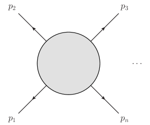
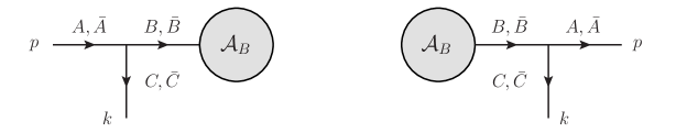
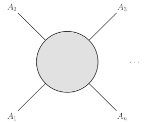
In this section, we examine the replica trick argument for soft gluon exponentiation, first presented in Refs. [125, 127]. Let us consider a scattering amplitude ${\cal A}_{n}$ with $n$ external partons and momenta labelled as shown in Fig. 1.

Refer to caption
Figure 1: An $n$-point scattering amplitude, where all external momenta have been taken to be outgoing.

As is well known, virtual QCD corrections to the amplitude lead to infrared (IR) singularities, associated with those kinematic regions in which the exchanged parton is soft (i.e. it has vanishing 4-momentum), or collinear to any of the hard external legs. The correction has a universal form, meaning that for a general amplitude it may be factorised according to the following schematic formula [143]

$${\cal A}_{n}(\{p_{i}\})=\left[{\cal H}_{n}(\{p_{i}\},\{n_{i}\})\otimes\,{\cal S}(\{\beta_{i}\})\right]\frac{\prod_{i=1}^{n}J(p_{i},n_{i})}{\prod_{i=1}^{n}{\cal J}(\beta_{i},n_{i})}\,.$$ (2.1)

Here ${\cal H}_{n}(\{p_{i}\},\{n_{i}\})$ is a process-dependent hard function, free of IR singularities. The soft function ${\cal S}(\{\beta_{i}\})$ depends only on the 4-velocities of the incoming and outgoing particles, and collects all singularities arising from soft radiation. This object is colour-connected to the hard function, as indicated by the symbol $\otimes$. The jet function $J(p_{i},n_{i})$ collects collinear singularities associated with emissions off the external leg with momentum $p_{i}$, and has a universal definition involving an auxiliary 4-vector $n_{i}$. Including both the soft and jet functions leads to a double-counting of radiation that is both soft and collinear, such that one has to remove each double-counted contribution. This is done though dividing out an eikonal jet function ${\cal J}(\beta_{i},n_{i})$ associated with leg $i$. The soft and (eikonal) jet functions all have universal definitions involving the appropriate partonic fields and Wilson line operators. Note that, given that the auxiliary vectors $\{n_{i}\}$ are arbitrary (apart from the condition $n_{i}\cdot p_{i}\neq 0$), dependence on them must cancel between the (eikonal) jet and hard functions, which in practice amounts to fixing the definition of the hard function in terms of the jet functions.

Eq. (2.1) is known as the soft-collinear factorisation formula, and simplifies considerably if one only cares about the leading IR singularities of a given amplitude. In that case, all radiation must be soft (and collinear) so that one may remove the (eikonal) jet functions. Furthermore, higher-order contributions to the hard function can be neglected, such that this may be replaced by its first-order approximation. Note that this approximation does not have to correspond to the leading-order (LO) of a given inclusive scattering process, depending on whether or not we are considering a subleading partonic channel that only turns on at next-to-leading order (NLO) or higher. Thus, Eq. (2.1) reduces to

$${\cal A}_{n}(\{p_{i}\})={\cal H}^{(0)}_{n}(\{p_{i}\})\,\otimes\,{\cal S}(\{\beta_{i}\})\,,$$ (2.2)

for some suitably defined first-order hard function ${\cal H}^{(0)}_{n}(\{p_{i}\})$ for an $n$-legged hard-scattering processes. Classifying the leading IR singularities then amounts to calculating the soft function, which has the following operator definition as a vacuum expectation value [143]:

$${\cal S}\equiv{\cal S}(\{\beta_{i}\})=\left\langle 0\left|\prod_{i=1}^{n}\Phi_{i}(A)\right|0\right\rangle$$ (2.3)

where

$$\Phi_{i}(A)={\cal P}\exp\left[ig_{s}\beta_{i}^{\mu}{\bf T}_{i}^{a}\int{\rm d}t_{i}A^{a}_{\mu}(t_{i}\beta_{i})\right],$$ (2.4)

is a Wilson line operator along the classical straight-line contour $x_{i}^{\mu}=t_{i}\beta_{i}^{\mu}$ of external parton $i$, with $\beta_{i}^{\mu}$ the relevant 4-velocity. Furthermore, ${\bf T}^{a}_{i}$ is a colour generator in the appropriate representation of hard line $i$, $g_{s}$ is the strong coupling, and ${\cal P}$ denotes path-ordering of these colour generators along the integration contour. We can formally write the vacuum expectation value in Eq. (2.3) as a path integral over the soft gauge field $A^{a}_{\mu}$ that couples to each external line:

$${\cal S}=\int[{\cal D}A]\,\prod_{i=1}^{n}{\cal P}\exp\left(ig_{s}\beta_{i}^{\mu}{\bf T}_{i}^{a}\int{\rm d}t_{i}A_{\mu}^{a}(t_{i}\beta_{i})\right)\,e^{iS[A]}\,,$$ (2.5)

where $S[A]$ is the action for the soft gauge field (note that this involves additional fields, which we have left implicit). Contracting the gluon fields with the action and carrying out the path integral (order-by-order) generates all possible Feynman diagrams in which the Wilson lines are connected by soft gluon graphs.

It is well-known that one may write the soft function in an exponential form, where the logarithm contains certain sets of diagrams known as webs. The concept of a web was first introduced in QCD in the case of processes involving two coloured particles only [10, 11, 12], but has more recently been generalised to arbitrary multiparton scattering processes [127] (see Refs. [136, 137] for reviews). This property may be derived using the replica trick. To this end, we start with ${\cal S}$ defined as in Eq. (2.5), and consider its counterpart in a distinct, duplicated theory that contains $N$ identical copies, or replicas, of the original soft gauge field. Let us label these different fields by $\{A_{\mu}^{{\color[rgb]{0,0,0}{(i)}}a}\}$, where ${\color[rgb]{0,0,0}{(i)}}$ is the replica index. The soft gauge fields of different replicas are required to be non-interacting, so that the action for the replicated theory can simply be expressed as the sum of actions $S[A_{\mu}^{{\color[rgb]{0,0,0}{(i)}}}]$ for each gauge field.444Note that in diagrams where gluons couple via other fields off the Wilson lines (e.g. to fermion bubbles), we must also replicate these other fields. We will not need to consider this complication explicitly here. The soft function in the replicated theory, denoted by $\color[rgb]{0,0,0}{{\cal S}_{N}}$, then takes the form

$\displaystyle\color[rgb]{0,0,0}{{\cal S}_{N}}$ $\displaystyle={\color[rgb]{0,0,0}{\prod_{i=1}^{N}}}\int[{\cal D}A^{{\color[rgb]{0,0,0}{(i)}}}]\,\prod_{j}^{n}\Phi_{j}(A^{{\color[rgb]{0,0,0}{(i)}}})\,e^{iS[A^{{\color[rgb]{0,0,0}{(i)}}}]}$ (2.6)
$\displaystyle={\cal S}^{N}.$

In the first line, we now have a product of Wilson lines on each parton leg: one for each replica number. In the second line, we have recognised that the soft function in the replicated theory amounts to the original soft function raised to the power $N$, and the non-interacting nature of the replicas (leading to additivity of their actions) is crucial in this regard. A simple mathematical identity allows us to write

$${\cal S}^{N}=1+N\log{\cal S}+{\cal O}(N^{2})\,,$$ (2.7)

from which we can immediately conclude that the logarithm of the soft function contains only those diagrams which in the replicated theory are ${\cal O}(N)$. This gives the following recipe for determining $\log{\cal S}$ (and thus the exponentiated soft function):

  1. 1.

    Draw all possible Feynman diagrams in the replicated theory. These consist of Feynman diagrams that also occur in the original theory, but where each gluon emitted from a Wilson line now carries a replica index.

  2. 2.

    Find the dependence of each diagram on the number of replicas $N$.

  3. 3.

    Take the ${\cal O}(N)$ part of each diagram, which gives the contribution of each diagram to the logarithm of the soft function.

By taking the exponent of the logarithm of the soft function one directly resums soft (and possibly collinear) eikonal emissions.

The simplest case to consider is that of QED. There are then no non-commuting colour matrices to worry about, and the soft function for the replicated theory reduces to

$\displaystyle{\color[rgb]{0,0,0}{{\cal S}_{N}}}=\left[{\color[rgb]{0,0,0}{\prod_{i=1}^{N}}}\int{\cal D}A^{{\color[rgb]{0,0,0}{(i)}}}\right]\left[\prod_{k=1}^{n}\exp\left(ie\,{\color[rgb]{0,0,0}{\sum_{j=1}^{N}}}\int{\rm d}x_{k}^{\mu}A^{{\color[rgb]{0,0,0}{(j)}}}_{\mu}(x_{k})\right)\right]\exp\left(i{\color[rgb]{0,0,0}{\sum_{l=1}^{N}}}S[A^{{\color[rgb]{0,0,0}{(l)}}}]\right).$ (2.8)

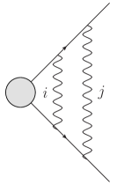
This generates Feynman diagrams where each external line can emit photons, which may be joined by other fields off the Wilson lines. If we consider a diagram such as that shown in Fig. 2, which has 2 connected soft photon subdiagrams, there are $N$ choices for the first replica index $i$, and $N$ choices for the second replica index $j$. The diagram is thus ${\cal O}(N^{2})$ and so does not contribute to the logarithm of the soft function. Likewise, a diagram with $m$ connected soft photon subdiagrams will be ${\cal O}(N^{m})$, such that only diagrams with a single connected piece $m=1$ contribute to the logarithm of the soft function. This is the well-known exponentiation of connected soft photon diagrams that was first derived a long time ago using combinatoric methods [144].

Refer to caption
Figure 2: A diagram occurring in the replicated soft photon theory of Eq. (2.8), for the case of two outgoing Wilson lines exchanging soft photons. There are two connected soft photon subdiagrams once the hard external lines are removed, consisting of individual soft photons, where $i$ and $j$ denote their replica indices.

Returning to a non-abelian context, we must face the fact that colour matrices associated with different replica fields do not commute with each other. To deal with this complication, Refs. [127, 125] noted that one may rewrite the replicated soft function of Eq. (2.6) in a form that instead makes clear the product of Wilson line operators associated with each individual hard leg $k$:

$\displaystyle{\color[rgb]{0,0,0}{{\cal S}_{N}}}$ $\displaystyle=\int[{\cal D}A^{{\color[rgb]{0,0,0}{(1)}}}]\ldots[{\cal D}A^{{\color[rgb]{0,0,0}{(N)}}}]\,e^{i{\color[rgb]{0,0,0}{\sum_{j=1}^{N}}}S[A^{{\color[rgb]{0,0,0}{(j)}}}]}\,\prod_{k=1}^{n}\left[\Phi_{k}(A^{{\color[rgb]{0,0,0}{(1)}}})\ldots\Phi_{k}(A^{{\color[rgb]{0,0,0}{(N)}}})\right].$ (2.9)

Here we have used the commuting nature of Wilson-line operators associated with different external legs, as they act on different partonic colour indices. Note that we are not allowed to reorder Wilson-line operators associated with the same leg, as they are non-commuting. There are then $N$ Wilson-line operators on each leg $k$, one for each replica gauge field, and such that the replica index increases as we go along the leg. Following Ref. [127, 125], we can implement this constraint in a convenient way by introducing a replica-ordering operator ${\cal R}$, such that the product of Wilson line operators on a given leg can be written

$$\prod_{{\color[rgb]{0,0,0}{j=1}}}^{\color[rgb]{0,0,0}{N}}{\cal P}\exp\left[ig_{s}\int{\rm d}x_{k}^{\mu}A_{\mu}^{{\color[rgb]{0,0,0}{(j)}}}\right]={\cal R}{\cal P}\exp\left[ig_{s}{\color[rgb]{0,0,0}{\sum_{j=1}^{N}}}\int{\rm d}x_{k}^{\mu}A_{\mu}^{{\color[rgb]{0,0,0}{(j)}}}(x_{k})\right].$$ (2.10)

On the right-hand side, we now have a single path-ordered exponential, but where, in performing the Taylor expansion, ${\cal R}$ acts to reorder colour matrices where necessary, such that the replica index is increasing along the line. To clarify this, the explicit action of ${\cal R}$ on two colour generators ${\bf T}_{k}^{{\color[rgb]{0,0,0}{(i)}}}$ and ${\bf T}_{k}^{{\color[rgb]{0,0,0}{(j)}}}$ associated with replica indices $i$ and $j$ is defined as

$${\cal R}\left[{\bf T}_{k}^{{\color[rgb]{0,0,0}{(i)}}}{\bf T}_{k}^{{\color[rgb]{0,0,0}{(j)}}}\right]=\begin{cases}{\bf T}_{k}^{{\color[rgb]{0,0,0}{(i)}}}{\bf T}_{k}^{{\color[rgb]{0,0,0}{(j)}}},\quad i\leq j\\ {\bf T}_{k}^{{\color[rgb]{0,0,0}{(j)}}}{\bf T}_{k}^{{\color[rgb]{0,0,0}{(i)}}},\quad i>j,\end{cases}$$ (2.11)

so that ${\cal R}$ reorders the matrices only if the replica numbers are not increasing. This definition is straightforward to generalise to higher numbers of colour matrices. Armed with the replica-ordering operator ${\cal R}$, our replicated soft function of Eq. (2.9) now assumes the form

$\displaystyle{\color[rgb]{0,0,0}{{\cal S}_{N}}}$ $\displaystyle=\int[{\cal D}A^{{\color[rgb]{0,0,0}{(1)}}}]\ldots[{\cal D}A^{{\color[rgb]{0,0,0}{(N)}}}]\,e^{i{\color[rgb]{0,0,0}{\sum_{j=1}^{N}}}S[A^{{\color[rgb]{0,0,0}{(j)}}}]}\,\left[\prod_{k=1}^{n}{\cal R}\,{\cal P}\,e^{ig_{s}\,{\color[rgb]{0,0,0}{\sum_{j=1}^{N}}}\int{\rm d}x_{k}^{\mu}A_{\mu}^{{\color[rgb]{0,0,0}{(j)}}}(x_{k})}\right].$ (2.12)

This provides a systematic prescription for ascertaining which diagrams contribute to the logarithm of the soft function. Contracting the fields within each replicated field theory leads to a set of Feynman diagrams. The colour factor of each such diagram will not be the usual colour factor of QCD perturbation theory, but will instead have colour matrices reordered by the operator ${\cal R}$. The contribution of each diagram in the replicated theory will depend upon the number of replicas $N$ in general. One may then take the ${\cal O}(N)$ part of each diagram as before.

Replica-ordering hierarchy $h$ ${\cal R}[C(a)|h]$ ${\cal R}[C(b)|h]$ Multiplicity
$i=j$ $C(a)$ $C(b)$ $N$
$i<j$ $C(a)$ $C(a)$ $N(N-1)/2$
$i>j$ $C(a)$ $C(a)$ $N(N-1)/2$
Table 1: Replica trick analysis of the diagrams in Fig. 3. For each diagram $D$ we give the various hierarchies $h$ of the ordering of the replica indices, together with the colour factor ${\cal R}[C(D)|h]$ one obtains by applying the replica-ordering operator ${\cal R}$. Finally, we give the number of ways of choosing replica numbers consistent with each hierarchy.
Refer to caption
Figure 3: Two diagrams that potentially contribute to the logarithm of the QCD soft function, involving two outgoing Wilson lines. Replica indices $i$ and $j$ are labelled, as are the numbers of the Wilson lines.

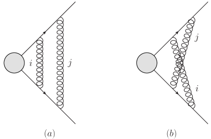
The simplest non-trivial example of this procedure is the case of two separate gluon emissions between two Wilson lines, for which the two Feynman diagrams in the replicated theory are shown in Fig. 3. To calculate the colour factors, we must take into account all possible hierarchies of replica numbers, given that ${\cal R}$ potentially acts differently in each case. For example, the colour factor of diagram (a) is

$${\cal R}\left[{\bf T}_{1}^{{\color[rgb]{0,0,0}{(i)}}}{\bf T}_{1}^{{\color[rgb]{0,0,0}{(j)}}}{\bf T}_{2}^{{\color[rgb]{0,0,0}{(i)}}}{\bf T}_{2}^{{\color[rgb]{0,0,0}{(j)}}}\right],$$ (2.13)

with ${\bf T}_{k}$ a general colour operator acting on the external line with label $k=1,2$. If $i=j$ or $i<j$, the replica ordering operator will leave the colour factor intact. If $i>j$, however, it will reorder the colour matrices on each line, so that one has

$${\cal R}\left[{\bf T}_{1}^{{\color[rgb]{0,0,0}{(i)}}}{\bf T}_{1}^{{\color[rgb]{0,0,0}{(j)}}}{\bf T}_{2}^{{\color[rgb]{0,0,0}{(i)}}}{\bf T}_{2}^{{\color[rgb]{0,0,0}{(j)}}}\right]=\left[{\bf T}_{1}^{{\color[rgb]{0,0,0}{(j)}}}{\bf T}_{1}^{{\color[rgb]{0,0,0}{(i)}}}{\bf T}_{2}^{{\color[rgb]{0,0,0}{(j)}}}{\bf T}_{2}^{{\color[rgb]{0,0,0}{(i)}}}\right],\quad i>j\,.$$ (2.14)

This has the same form as the original colour factor with the indices $i$ and $j$ interchanged, and so for all hierarchies of replica number, we obtain the colour factor of diagram (a). For a given hierarchy of replica orderings $h$ and diagram $D$, we denote the replica-ordered colour factor by ${\cal R}[C(D)|h]$. We may then summarise the above analysis as in table 1, which gives the different hierarchies of the ordering of the two replica indices $i$ and $j$, together with the colour factor obtained by applying the replica ordering operator in each case. The table also details the findings for diagram (b). For this diagram, for some hierarchies, the action of ${\cal R}$ is to disentangle the crossed gluon pair, thus creating the colour factor of diagram (a). Finally, we give the multiplicity factor corresponding to the number of ways of choosing replica numbers consistent with the given hierarchy. The total contribution of a given diagram $D$ in the replicated theory will be given by its kinematic factor ${\cal K}(D)$, multiplied by the various colour factors weighted by the appropriate multiplicities. For diagram (a), for example, we have

$\displaystyle{\cal K}(a)C_{N}(a)\,,\quad C_{N}(a)=NC(a)+2C(a)\left(\frac{N(N-1)}{2}\right)=N^{2}C(a)\,,$ (2.15)

where $C_{N}(D)$ denotes the effective colour factor for diagram $D$. According to the replica trick, we must take the ${\cal O}(N)$ part of this as the contribution to the logarithm of the soft function, and following Ref. [127] we may write this as

$${\cal K}(D)\tilde{C}(D),\quad\tilde{C}(D)\equiv C_{N}(D)\Big{|}_{{\cal O}(N)}.$$ (2.16)

For the case of diagram (a), we thus find $\tilde{C}(a)=0$. In the case of diagram (b), we instead find

$\displaystyle\tilde{C}(b)=C(b)-C(a)\,,$ (2.17)

such that this diagram indeed contributes to the logarithm of the soft function. It does so, however, with a modified colour weight, and this is a special case of the previously known fact that in two-parton processes, only those diagrams which are two-particle irreducible (i.e. webs) exponentiate [10, 11, 12], with appropriately modified colour factors. In general, we find then the exponentiated soft function can be written as

$\displaystyle\mathcal{S}={\rm exp}\left[\sum_{D}\mathcal{K}(D)\,\tilde{C}(D)\right],$ (2.18)

where the argument of the exponent are the so-called web diagrams.

The above methods generalise to arbitrary multiparton scattering processes in QCD, where the simple criterion of two-particle irreducibility no longer applies. It is nevertheless possible to write a general structure for the logarithm of the soft function. To do so, note that the ${\cal R}$ operator reorders gluon attachments on all external legs, so that the exponentiated colour factor of a given diagram potentially depends on all other diagrams related by gluon permutations. There is a closed set of such permutations (as exemplified by the diagrams of Fig. 3), and Ref. [127] defined a multiparton web to consist of such a closed set of diagrams. This interpretation survives after the effects of renormalisation are taken into account [129], and a further refinement of this notion has been introduced in Refs. [138, 139]. In general, the exponentiated colour factor of a diagram $D$ in each web $W$ will be a superposition of all colour factors in the web

$$\tilde{C}(D)=\sum_{D^{\prime}\in W}R_{DD^{\prime}}\,C(D^{\prime})\,.$$ (2.19)

Here the quantity $R_{DD^{\prime}}$ is known as a web mixing matrix. It has a purely combinatorial definition [130], of interdisciplinary interest [145, 146], and which has been further explored in Refs. [131, 138, 139]. Combining the exponentiated colour factor of each diagram with its kinematic part, the contribution of a given web to the logarithm of the soft function is

$$w=\sum_{D,D^{\prime}\in W}{\cal K}(D)\,R_{DD^{\prime}}\,C(D^{\prime})\,.$$ (2.20)

So far we have only considered virtual emissions. Comments regarding the generalisation to real emissions were made in Ref. [83], which postulates a soft function at the level of the squared amplitude/cross-section. That is, one may write

$${\cal S}(\bar{v})=\sum_{m}{\rm Tr}\left[\Big{\langle}0\Big{|}\Phi_{1}\ldots\Phi_{n}\Big{|}m\Big{\rangle}\Big{\langle}m\Big{|}\Phi_{n}^{\dagger}\ldots\Phi_{1}^{\dagger}\Big{|}0\Big{\rangle}\right]\delta(v(m)-\bar{v})\,.$$ (2.21)

Here the trace is over the colour indices of the outgoing parton legs, and the two vacuum expectation values (VEVs) are taken between a vacuum state, and a final state $|m\rangle$ containing $m$ soft gluons together with a measurement function $\delta(v(m)-\bar{v})$ corresponding to the (dimensionless) observable $\bar{v}$ and the $m$-particle definition of that observable. We use a compact notation for the sum over final states, which implicitly contains the integral over the combined phase space of the hard partons and soft gluons for each $m$.555For particular scattering processes in the literature, the precise definition of the soft function may vary, depending on whether it is defined for the squared amplitude or a normalised differential cross-section. It is possible to write a formal generating functional for soft functions such as those in Eq. (2.21) which allows to apply the replica trick directly, although this was not proven in Ref. [83]. We thus return to this point in what follows.

In this section, we have reviewed how the replica trick can be used to show how soft gluon emissions exponentiate. It is perhaps more correct to say that the replica trick constitutes a systematic procedure for determining the logarithm of the soft function. Scrutiny of the above arguments, however, reveals that they do not crucially depend on the nature of the Wilson lines in Eq. (2.5). We are free to replace the latter with a generalised soft-emission operator, and indeed Ref. [125] did precisely this in arguing that certain classes of next-to-soft contributions formally exponentiate. Here, we will seek a different generalised soft-emission line, which includes the effects of soft quark emission. This is the subject of the following section.

3 The replica trick for generalised soft-parton emissions

The replica trick may be extended to show that not only soft-gluon, but also soft-quark emissions can be exponentiated. Indeed, in applying the replica trick to prove the exponentiation of soft gluons, the precise definition of the Wilson line (and all its gauge-transformation properties) never entered. All that matters is that we are able to write down an operator definition that generates the soft emissions in QCD up to all orders in the strong coupling. When considering also the emission of soft quarks, we must apply a similar argument, but the difficulty lies in finding a suitable replacement for the operator that describes the emission of soft (anti-)quarks in addition to gluons. We will successfully seek such a generalised soft-emission operator below. Our strategy to prove that soft quark emissions exponentiates consists of three key ingredients:

  1. 1.

    We will consider a hard external leg of an amplitude, and show that the emission of a single soft (anti-)quark or gluon can be written in terms of universal emission factors (Section 3.1). The latter have been considered in Ref. [79], and we build on those results here.

  2. 2.

    These emission factors are used to build a generalised soft-emission operator for the emission of arbitrary numbers of soft partons from a hard leg (Section 3.2).

  3. 3.

    The generalised soft-emission operator is used to define a generalised soft function, which captures all soft parton emissions. This generalised soft function will have a path integral representation, allowing the replica trick to be used in an analogous fashion to the case of soft gluon emission (Section 3.3).

In carrying out this programme, we will also provide a more rigorous treatment of the replica trick for real emissions than has previously appeared in the literature.

3.1 Emission factors for soft partons

Refer to caption
Figure 4: Emission of various soft partons from incoming hard legs, where $A_{X}$ denotes the amplitude with an incoming parton $X$, but where the external wavefunction for the particle $X$ is removed. Here $\{i,j,\dots\}$ ($\{a,b,c,\dots\})$ represent the fundamental (adjoint) colour indices, while Lorentz and spinor indices are suppressed, though explicitly written in the corresponding Eqs. (3.1) – (3.7).

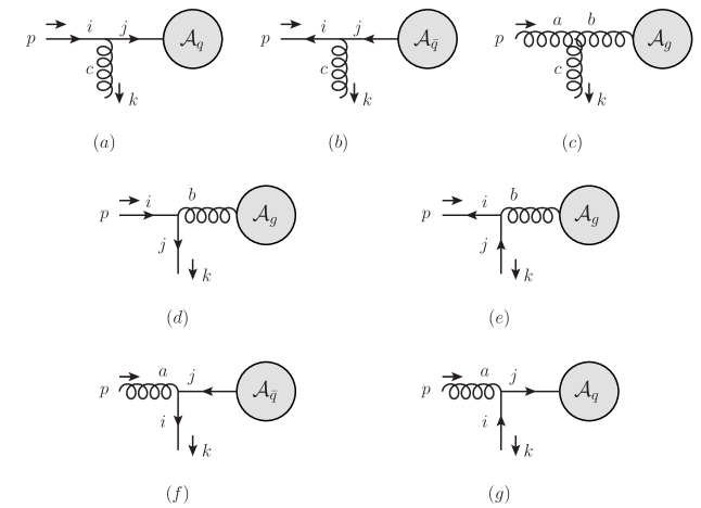
Consider the emission of a soft gluon from an incoming quark leg, as shown in Fig. 4(a). Scaling the gluon momentum with $k^{\mu}\to\lambda k^{\mu}$ and taking $\lambda\to 0$ leads to the well-known eikonal Feynman rule, such that the matrix element for diagram (a) is written as

$$[\mathcal{M}_{q}^{\rm in}(p)]^{c}_{\mu}=\frac{g_{s}}{p\cdot k}\,[\mathcal{A}_{q}(p)]_{\hat{b}}^{j}\,t_{ji}^{c}\left(p_{\mu}\delta_{\hat{b}\hat{a}}\right)u^{i}_{\hat{a}}(p)\,.$$ (3.1)

Here $\mathcal{A}_{q}(p)$ denotes the amplitude for an incoming quark leg with the external spinor removed. We denote spinor indices by hatted lower-case Latin letters $\{\hat{a},\hat{b},\dots\}$ (raised or lowered spinor indices carry no meaning). The fundamental (adjoint) colour indices are denoted with $\{i,j,\dots\}$ ($\{a,b,c,\dots\})$. The colour generator of the ${\rm SU}(3)$ gauge group in the fundamental representation is denoted by $t^{a}_{ij}$. The external wavefunction of the quark carries a label $i$, which refers to the colour of the incoming quark, whereas the amplitude carries the label $j$, referring to the colour of the internal quark entering the hard scattering. We have not included an external particle wavefunction for the emitted soft gluon, leaving open the possibility of this gluon being either real or virtual.

Similarly, if the emitting particle were an anti-quark instead of a quark (diagram (b)) we would have

$$[\mathcal{M}_{\bar{q}}^{\rm in}(p)]^{c}_{\mu}=\frac{g_{s}}{p\cdot k}\,\bar{v}^{i}_{\hat{a}}(p)\,(-t_{ij}^{c})\,\left(p_{\mu}\delta_{\hat{a}\hat{b}}\right)\,[\mathcal{A}_{\bar{q}}(p)]^{j}_{\hat{b}}\,.$$ (3.2)

Performing the same exercise for diagram (c) leads to

$$[\mathcal{M}_{g}^{\rm in}(p)]^{c}_{\mu}=\frac{g_{s}}{p\cdot k}\,if^{bca}\left(p_{\mu}\eta^{\alpha\beta}\right)[\mathcal{A}_{g}(p)]_{\beta}^{b}\,\epsilon_{\alpha}^{a}(p)\,,$$ (3.3)

with $f^{abc}$ the colour generator of the ${\rm SU}(3)$ gauge group in the adjoint representation.

To obtain the Feynman rules for the emission of a soft-quark (soft anti-quark) from an incoming quark (anti-quark), we may, in analogy with the soft-gluon case, scale the (anti-)quark momentum with $k^{\mu}\to\lambda k^{\mu}$ and take $\lambda\to 0$ [79]. The soft (anti-)quark emission contributions from a quark (anti-quark) are shown respectively in diagrams (d) and (e) of Fig. 4. We obtain

$\displaystyle[\mathcal{M}_{q}^{\rm in}(p)]^{j}_{\hat{c}}$ $\displaystyle=\frac{g_{s}}{p\cdot k}\,t^{b}_{ji}\left(-\frac{1}{2}\gamma^{\beta}_{\hat{c}\hat{a}}\right)u^{i}_{\hat{a}}(p)\,[\mathcal{A}_{g}(p)]_{\beta}^{b}\,,$ (3.4)
$\displaystyle[\mathcal{M}_{\bar{q}}^{\rm in}(p)]^{j}_{\hat{c}}$ $\displaystyle=\frac{g_{s}}{p\cdot k}\,\bar{v}^{i}_{\hat{a}}(p)\,t^{b}_{ij}\left(-\frac{1}{2}\gamma^{\beta}_{\hat{a}\hat{c}}\right)[\mathcal{A}_{g}(p)]_{\beta}^{b}\,.$ (3.5)

Finally, the case of a soft quark (soft anti-quark) emission from an incoming gluon, shown respectively in diagrams (f) and (g) of Fig. 4, reads

$\displaystyle[\mathcal{M}_{g}^{\rm in}(p)]^{i}_{\hat{c}}$ $\displaystyle=\frac{g_{s}}{p\cdot k}\,(-t^{a}_{ij})\,\frac{1}{2}\big{(}\gamma^{\alpha}\not{p}\big{)}_{\hat{c}\hat{b}}\,[\mathcal{A}_{\bar{q}}(p)]^{j}_{\hat{b}}\,\epsilon^{a}_{\alpha}(p)\,,$ (3.6)
$\displaystyle[\mathcal{M}_{g}^{\rm in}(p)]^{i}_{\hat{c}}$ $\displaystyle=\frac{g_{s}}{p\cdot k}\,[\mathcal{A}_{q}(p)]_{\hat{b}}^{j}\,t^{a}_{ji}\,\frac{1}{2}\big{(}\not{p}\gamma^{\alpha}\big{)}_{\hat{b}\hat{c}}\,\epsilon^{a}_{\alpha}(p)\,.$ (3.7)
Refer to caption
Figure 5: Emission of a parton with (spinor/vector) index $C$ from two partons with indices $B$ and $A$. The barred letters denote colour indices.

In each case, the additional factors in the amplitude take the form of an eikonal denominator depending on the soft momentum $k$, with everything else depending only on the hard momentum $p$. The additional factors are sandwiched between the non-radiative amplitude on the one-hand, and the external wavefunction for the hard leg on the other, meaning we can write a general form that covers all cases. Let us first introduce an array of fields

$$\left[\Theta_{I}\right]^{\bar{A}}_{A}\equiv(\psi^{i}_{\hat{a}},\bar{\psi}^{i}_{\hat{a}},A^{a}_{\alpha})\,,$$ (3.8)

where $\psi^{i}$ ($\bar{\psi}^{i}$) denotes the (anti-)quark field, and $i$, $a$ are colour labels. On the left-hand side, we have introduced a flavour index $I\in\{q,\bar{q},g\}$, and an index $A$ in Minkowski/spinor space, labeling the correct index for the relevant fields (i.e. $A\in\{\hat{a},\hat{a},\alpha\}$). Furthermore, the index $\bar{A}$ labels the colour index associated with the field whose species index is $A$: $\bar{A}\in\{i,i,a\}$. We stress that this is purely a book-keeping device that is useful for our purposes – we do not wish to imply that these fields form a multiplet that is acted upon by any sort of symmetry transformation (as would be the case in e.g. a supersymmetric theory). Next, using the same basis, let us define an array of external initial-state particle wavefunctions that go with the fields of Eq. (3.8)

$$\left[\xi_{I}\right]^{\bar{A}}_{A}=(u^{i}_{\hat{a}},\bar{v}^{i}_{\hat{a}},\epsilon^{a}_{\alpha})\,.$$ (3.9)

We will also need an array corresponding to the various wave-function stripped amplitudes occurring in Fig. 4

$$\left[\mathcal{A}_{I}\right]^{\bar{A}}_{A}=\left([\mathcal{A}_{q}(p)]^{i}_{\hat{a}},[\mathcal{A}_{\bar{q}}(p)]^{i}_{\hat{a}},[\mathcal{A}_{g}(p)]^{a}_{\alpha}\right).$$ (3.10)

In this notation, we may summarise Eqs. (3.1)–(3.7) in a compact notation by introducing a transition matrix for soft emissions off incoming hard partons, $[{\cal T}^{\rm in}_{IJ}(p)]^{\bar{C},\bar{A}\bar{B}}_{C,AB}$, such that

$$[\mathcal{M}_{I}^{\rm in}(p)]_{C}^{\bar{C}}=\frac{g_{s}}{p\cdot k}\,[\xi_{I}(p)]^{\bar{A}}_{A}\,[{\cal T}^{\rm in}_{IJ}(p)]^{\bar{C},\bar{A}\bar{B}}_{C,AB}\,[\mathcal{A}_{J}(p)]^{\bar{B}}_{B}\,,$$ (3.11)

with666Note that the indices $I$,$J$ in Eq. (3.12) are not summed, i.e. there is no matrix multiplication in the indices $I$,$J$. These simply labels the flavour of the transitions, both on the l.h.s and the r.h.s of Eq. (3.12).

$$[{\cal T}^{\rm in}_{IJ}(p)]^{\bar{C},\bar{A}\bar{B}}_{C,AB}=[{\bf T}_{IJ}]^{\bar{C}}_{\bar{A}\bar{B}}\,[Q^{\rm in}_{IJ}(p)]_{C,AB}.$$ (3.12)

The labeling is defined such that it follows the momentum flow of the hard line, which goes from $A$ to $B$. One sees that this object consists of a kinematic part $[Q^{\rm in}]_{C,AB}$ and a colour factor ${\bf T}^{\bar{C}}_{\bar{A}\bar{B}}$. In the basis Eq. (3.10) we may write

$$[{\cal T}^{\rm in}(p)]^{\bar{C},\bar{A}\bar{B}}_{C,AB}=\left(\begin{array}[]{ccc}[{\cal T}_{qq}^{\rm in}(p)]^{c,ij}_{\gamma,\hat{a}\hat{b}}&0&[{\cal T}_{qg}^{\rm in}(p)]^{k,ib}_{\hat{c},\hat{a}\beta}\\ 0&[{\cal T}_{\bar{q}\bar{q}}^{\rm in}(p)]^{c,ij}_{\gamma,\hat{a}\hat{b}}&[{\cal T}_{\bar{q}g}^{\rm in}(p)]^{k,ib}_{\hat{c},\hat{a}\beta}\\ ({\cal T}_{gq}^{\rm in}(p))^{k,aj}_{\hat{c},\alpha\hat{b}}&[{\cal T}_{g\bar{q}}^{\rm in}(p)]^{k,aj}_{\hat{c},\alpha\hat{b}}&[{\cal T}_{gg}^{\rm in}(p)]^{c,ab}_{\gamma,\alpha\beta}\end{array}\right),$$ (3.13)

where we will refer to the entries of this matrix as emission factors, and where we have explicitly indicated where no valid non-zero entry is possible. The assignment of the colour factor $[{\bf T}_{IJ}]^{\bar{C}}_{\bar{A}\bar{B}}$ follows the usual eikonal Feynman rules. In our notation, we have used the colour labels $a,b$ ($c$) for colour indices of hard (soft) gluons, and $i,j$ ($k$) for that of hard (soft) quarks and anti-quarks. The assignment of the kinematic factor $[Q^{\rm in}]_{C,AB}$ can be inferred by direct comparison with Eqs. (3.1)–(3.7), and is summarised in Appendix A. Combining the colour and kinematic factors we find for the transition matrix

$$[{\cal T}^{\rm in}(p)]^{\bar{C},\bar{A}\bar{B}}_{C,AB}=\left(\begin{array}[]{ccc}t_{ji}^{c}\left(p_{\gamma}\delta_{\hat{b}\hat{a}}\right)&0&t^{b}_{ki}\left(-\frac{1}{2}\gamma^{\beta}_{\hat{c}\hat{a}}\right)\\ 0&(-t_{ij}^{c})\,\left(p_{\gamma}\delta_{\hat{a}\hat{b}}\right)&t^{b}_{ik}\left(-\frac{1}{2}\gamma^{\beta}_{\hat{a}\hat{c}}\right)\\ t^{a}_{jk}\,\frac{1}{2}\big{(}\not{p}\gamma^{\alpha}\big{)}_{\hat{b}\hat{c}}&(-t^{a}_{kj})\,\frac{1}{2}\big{(}\gamma^{\alpha}\not{p}\big{)}_{\hat{c}\hat{b}}&if^{bca}\left(p_{\gamma}\eta^{\beta\alpha}\right)\end{array}\right).$$ (3.14)

To summarise, in Eq. (3.11) we introduced a compact notation for the emission of a single soft parton with Lorentz/spinor and colour indices $C,\bar{C}$ off a hard incoming line with flavour $I$, space-time index $A$, and colour index $\bar{A}$. This hard parton then continues with internal flavour index $J$, space-time index $B$ and colour index $\bar{B}$. The notation in Eq. (3.11) is also illustrated in Fig. 5. We do not include an external wave-function for the emitted soft parton, leaving open the possibility of this parton being either real or virtual. Multiple soft emissions off a single hard parton can easily be described through repeated insertion of the transition matrix, where care of course has to be taken that the eikonal pre-factor $1/p\cdot k$ is updated accordingly. The final product of transition matrices may in the end then be sandwiched between a hard matrix element on one end, and the external wave function for the hard parton on the other. This will be demonstrated in Section 3.2.

One may perform the same exercise for a final-state emitter with hard momentum $p^{\mu}$. We may summarise the results as

$$[\mathcal{M}_{I}^{\rm out}(p)]_{C}^{\bar{C}}=\frac{g_{s}}{p\cdot k}\,[\bar{\xi}_{I}(p)]^{\bar{A}}_{A}\,[{\cal T}^{\rm out}_{IJ}(p)]^{\bar{C},\bar{A}\bar{B}}_{C,AB}\,[\mathcal{A}_{J}(p)]^{\bar{B}}_{B}\,,$$ (3.15)

The outgoing wave function can be any of

$$\left[\bar{\xi}_{I}\right]^{\bar{A}}_{A}=(\bar{u}^{j}_{\hat{a}},v^{j}_{\dot{a}},\epsilon^{\dagger a}_{\alpha})\,.$$ (3.16)

The transition matrix now describes soft emissions off hard outgoing partons, and can be written as

$$[{\cal T}^{\rm out}(p)]^{\bar{C},\bar{A}\bar{B}}_{C,AB}=\left(\begin{array}[]{ccc}[{\cal T}_{qq}^{\rm out}(p)]^{c,ij}_{\gamma,\hat{a}\hat{b}}&0&[{\cal T}_{qg}^{\rm out}(p)]^{k,ib}_{\hat{c},\hat{a}\beta}\\ 0&[{\cal T}_{\bar{q}\bar{q}}^{\rm out}(p)]^{c,ij}_{\gamma,\hat{a}\hat{b}}&[{\cal T}_{\bar{q}g}^{\rm out}(p)]^{k,ib}_{\hat{c},\hat{a}\beta}\\ ({\cal T}_{gq}^{\rm out}(p))^{k,aj}_{\hat{c},\alpha\hat{b}}&[{\cal T}_{g\bar{q}}^{\rm out}(p)]^{k,aj}_{\hat{c},\alpha\hat{b}}&[{\cal T}_{gg}^{\rm out}(p)]^{c,ab}_{\gamma,\alpha\beta}\end{array}\right),$$ (3.17)

Again, the colour factor follows the rules for eikonal emissions listed above. Together with the kinematic factor $\left[Q^{\rm out}\right]_{C,AB}$ (written out explicitly in Appendix A for all cases) we then obtain

$$[{\cal T}^{\rm out}(p)]^{\bar{C},\bar{A}\bar{B}}_{C,AB}=\left(\begin{array}[]{ccc}(-t_{ij}^{c})\left(p_{\gamma}\delta_{\hat{b}\hat{a}}\right)&0&t^{b}_{ik}\left(\frac{1}{2}\gamma^{\beta}_{\hat{a}\hat{c}}\right)\\ 0&t_{ji}^{c}\,\left(p_{\gamma}\delta_{\hat{b}\hat{a}}\right)&t^{b}_{ki}\left(\frac{1}{2}\gamma^{\beta}_{\hat{c}\hat{a}}\right)\\ (-t^{a}_{kj})\,\frac{1}{2}\big{(}\gamma^{\alpha}\not{p}\big{)}_{\hat{c}\hat{b}}&(t^{a}_{jk})\,\frac{1}{2}\big{(}\not{p}\gamma^{\alpha}\big{)}_{\hat{b}\hat{c}}&if^{acb}\left(p_{\gamma}\eta^{\alpha\beta}\right)\end{array}\right).$$ (3.18)

It is easy to check that $[{\cal T}^{\rm out}(p)]^{\bar{C},\bar{A}\bar{B}}_{C,AB}=[\overline{{\cal T}}^{\rm in}(p)]^{\bar{C},\bar{B}\bar{A}}_{C,BA}$, as required. We may now work towards a generalisation of the conventional Wilson lines, that includes emission of any soft partons. Let us start from the case of emission from an incoming line. In momentum space, the Feynman rule describing this process is given in Eq. (3.11), i.e.

$$\frac{g_{s}}{p\cdot k}\,\left[{\cal T}^{\rm in}\right]^{\bar{C},\bar{A}\bar{B}}_{C,AB},$$ (3.19)

which is sandwiched between the external incoming wave function $\xi^{\bar{A}}_{A}$ and the stripped hard-scattering amplitude ${\cal A}^{\bar{B}}_{B}$. In position space this Feynman rule reads

$\displaystyle ig_{s}\int_{-\infty}^{0}\,{\rm d}t\,\left[{\cal T}^{\rm in}\right]^{\bar{C},\bar{A}\bar{B}}_{C,AB}\,\Theta^{\bar{C}}_{C}(tp)\,e^{\varepsilon t}\,.$ (3.20)

The integral is defined over the incoming particle contour (parameterised by $x^{\mu}=tp^{\mu}$), and the factor $e^{\varepsilon t}$ makes sure the integral converges. To see the equivalence between the two Feynman rules, we may write the field in momentum space via the Fourier transform

$$\Theta^{\bar{C}}_{C}(x)=\int\frac{{\rm d}^{d}k}{(2\pi)^{d}}\,\tilde{\Theta}^{\bar{C}}_{C}(k)\,e^{ik\cdot x}=\int\frac{{\rm d}^{d}k}{(2\pi)^{d}}\,\tilde{\Theta}^{\bar{C}}_{C}(k)\,e^{it(k\cdot p)}.$$ (3.21)

Inserting this into Eq. (3.20) yields

$\displaystyle ig_{s}\int_{-\infty}^{0}{\rm d}t\,\left[{\cal T}^{\rm in}\right]^{\bar{C},\bar{A}\bar{B}}_{C,AB}\int\frac{{\rm d}^{d}k}{(2\pi)^{d}}\tilde{\Theta}^{\bar{C}}_{C}(k)\left[\frac{e^{it(k\cdot p)+t\varepsilon}}{ik\cdot p+\varepsilon}\right]^{0}_{-\infty}=\int\frac{{\rm d}^{d}k}{(2\pi)^{d}}\tilde{\Theta}^{\bar{C}}_{C}(k)\left[\frac{g_{s}}{p\cdot k-i\varepsilon}\left[{\cal T}^{\rm in}\right]^{\bar{C},\bar{A}\bar{B}}_{C,AB}\right],$ (3.22)

where the lower limit of the $t$ integral vanishes because of the $\varepsilon$ regulator. The contents of the square bracket is the required momentum-space Feynman rule, which indeed agrees with Eq. (3.19). We may define Feynman rules for outgoing emissions analogously, sending $\varepsilon\to-\varepsilon$ to make the integral well-defined. To further clarify Eq. (3.20), note that for the diagonal elements of $\left[{\cal T}^{\rm in}\right]^{\bar{C},\bar{A}\bar{B}}_{C,AB}$ (i.e. soft gluon emission), we may simplify it to

$\displaystyle ig_{s}{\bf T}^{c}\int_{-\infty}^{0}\,{\rm d}t\,p^{\mu}\,A^{c}_{\mu}(tp)\,,$ (3.23)

which is the usual exponent of the Wilson-line operator (see Eq. (2.4)), omitting the explicit identity matrices $\delta^{\hat{a}\hat{b}}$ and $\eta^{\alpha\beta}$ in spinor/Lorentz space. This is as it should be: the effect of a single gluon emission should be given by a Wilson line. However, this also suggests an interpretation of Eq. (3.20): it acts as a generalised Wilson line exponent that describes the emission of soft (anti-)quarks in addition to gluons. That we can indeed interpret the object in Eq. (3.20) in this way is discussed in the following section.

3.2 Multiple emissions from a generalised soft-emission operator

The effect of multiple emissions off a single (possibly flavour-changing) hard line with momentum $p^{\mu}$ may be generated by the following path-ordered object:

$${\cal F}^{\bar{A}\bar{B}}_{AB}={\cal P}\exp\left[ig_{s}\int_{-\infty}^{0}{\rm d}t\,\left[{\cal T}\right]^{\bar{C}}_{C}\,\Theta^{\bar{C}}_{C}(tp)\right]^{\bar{A}\bar{B}}_{AB}.$$ (3.24)

We will call this a generalised soft-emission operator. It carries open indices and needs to be sandwiched in-between the matrix element that the hard line originated from, and its external state. The notation of Eq. (3.24) is appropriate for an incoming hard line, and the regularisation is implicitly understood. The soft-emission operator for an outgoing hard line is easily obtained by switching the integration boundaries to $(0,\infty)$, and adapting the regularisation accordingly. To see that the object defined in Eq. (3.24) indeed defines multiple insertions of the transition matrix, we may expand it and examine the $\mathcal{O}(g_{s}^{l})$ contribution, which is given by

$${\cal F}^{\bar{A}\bar{B}}_{AB}\Big{|}_{\mathcal{O}(g_{s})^{l}}=(ig_{s})^{l}\int_{-\infty}^{0}{\rm d}t_{1}\,\left[{\cal T}\right]^{\bar{C}_{1},\bar{A}\bar{A}_{1}}_{C_{1},AA_{1}}\Theta^{\bar{C}_{1}}_{C_{1}}(t_{1}p)\,\,\dots\,\,\int_{t_{l-1}}^{0}{\rm d}t_{l}\,\left[{\cal T}\right]^{\bar{C}_{l},\bar{A}_{l-1}\bar{B}}_{C_{l},A_{l-1}B}\Theta^{\bar{C}_{l}}_{C_{l}}(t_{l}p)\,.$$ (3.25)

Writing again the field in momentum space through Eq. (3.21), we end up with a string of integrals of the form

$$\int_{-\infty}^{0}{\rm d}t_{1}\int_{t_{1}}^{0}{\rm d}t_{2}\,\,\dots\,\,\int_{t_{l-1}}^{0}{\rm d}t_{l}\,\exp\left[i\sum_{j=1}^{l}(k_{j}\cdot p)t_{j}\right]=\frac{(-i)^{l}}{k_{1}\cdot p\,(k_{1}+k_{2})\cdot p\,\dots\,(k_{1}+\dots+k_{l})\cdot p}\,,$$ (3.26)

where $k_{j}$ is the four-momentum of each of the soft fields. With this, the full soft-emission operator at $\mathcal{O}(g_{s}^{l})$ becomes

$${\cal F}^{\bar{A}\bar{B}}_{AB}\Big{|}_{\mathcal{O}(g_{s})^{l}}=\prod_{j=1}^{l}\left[\int\frac{{\rm d}^{d}k_{j}}{(2\pi)^{d}}\widetilde{\Theta}^{\bar{C}_{l}}_{C}(k_{j})\right]\frac{g_{s}^{l}}{k_{1}\cdot p\,\dots\,(k_{1}+\dots k_{l})\cdot p}\left[{\cal T}\right]^{\bar{C}_{1},\bar{A}\bar{A}_{1}}_{C_{1},AA_{1}}\,\dots\,\left[{\cal T}\right]^{\bar{C}_{l},\bar{A}_{l-1}\bar{B}}_{C_{l},A_{l-1}B}\,.$$ (3.27)

We may now see how one may use this object to generate soft emissions. For instance, we can consider a configuration involving an incoming quark with colour label $i_{1}$ and spinor label $\hat{a}_{1}$, transitioning into a gluon of colour index $b$, and space-time index $\beta$, entering into the hard scattering ${\cal A}_{g}$, at third order in the strong coupling $g_{s}$. The expansion of the generalised Wilson line up to third order automatically generates all contributions given in Figs. 6 and 7, given that the transitions operators ${\cal T}_{IJ}$ are matrices in the flavour space $IJ$, and matrix multiplication generates all possible transitions.
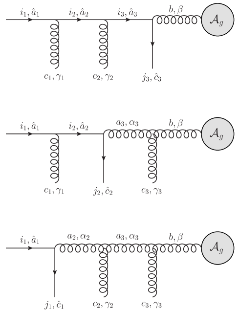
Refer to caption
Figure 6: Diagrams corresponding to the first three contributions in Eq. (3.28), originating from expanding the generalised Wilson line in Eq. (3.24) to third order in $g_{s}$, and selecting the components giving rise to a transition between an initial quark and a gluon incoming into the amplitude ${\cal A}_{g}$.

We obtain

$\displaystyle\frac{g_{s}^{3}}{p\cdot k_{1}\,p\cdot(k_{1}+k_{2})\,p\cdot(k_{1}+k_{2}+k_{3})}u^{i_{1}}_{\hat{a}_{1}}(p)\Big{\{}\left[{\cal T}^{{\rm in}}_{qq}(p)\right]^{c_{1},i_{1}i_{2}}_{\gamma_{1},\hat{a}_{1}\hat{a}_{2}}\,\left[{\cal T}^{\rm in}_{qq}(p)\right]^{c_{2},i_{2}i_{3}}_{\hat{c}_{2},\hat{a}_{2}\hat{a}_{3}}\,\left[{\cal T}^{\rm in}_{qg}(p)\right]^{j_{3},i_{3}b}_{\hat{c}_{3},\hat{a}_{3}\beta}$ (3.28)
$\displaystyle+\,\left[{\cal T}^{{\rm in}}_{qq}(p)\right]^{c_{1},i_{1}i_{2}}_{\gamma_{1},\hat{a}_{1}\hat{a}_{2}}\,\left[{\cal T}^{\rm in}_{qg}(p)\right]^{j_{2},i_{2}a_{3}}_{\hat{c}_{2},\hat{a}_{2}\alpha_{3}}\,\left[{\cal T}^{\rm in}_{gg}(p)\right]^{c_{3},a_{3}b}_{\gamma_{3},\alpha_{3}\beta}$
$\displaystyle+\,\left[{\cal T}^{{\rm in}}_{qg}(p)\right]^{j_{1},i_{1}a_{2}}_{\hat{c}_{1},\hat{a}_{1}\alpha_{2}}\,\left[{\cal T}^{\rm in}_{gg}(p)\right]^{c_{2},a_{2}a_{3}}_{\gamma_{2},\alpha_{2}\alpha_{3}}\,\left[{\cal T}^{\rm in}_{gg}(p)\right]^{c_{3},a_{3}b}_{\gamma_{3},\alpha_{3}\beta}$
$\displaystyle+\,\left[{\cal T}^{{\rm in}}_{qg}(p)\right]^{j_{1},i_{1}a_{2}}_{\hat{c}_{1},\hat{a}_{1}\alpha_{2}}\,\left[{\cal T}^{\rm in}_{gq}(p)\right]^{j_{2},a_{2}i_{3}}_{\hat{c}_{2},\alpha_{2}\hat{a}_{3}}\,\left[{\cal T}^{\rm in}_{qg}(p)\right]^{j_{3},i_{3}b}_{\hat{c}_{3},\hat{a}_{3}\beta}$
$\displaystyle+\,\left[{\cal T}^{{\rm in}}_{qg}(p)\right]^{j_{1},i_{1}a_{2}}_{\hat{c}_{1},\hat{a}_{1}\alpha_{2}}\,\left[{\cal T}^{\rm in}_{g\bar{q}}(p)\right]^{j_{2},a_{2}i_{3}}_{\hat{c}_{2},\alpha_{2}\hat{a}_{3}}\,\left[{\cal T}^{\rm in}_{\bar{q}g}(p)\right]^{j_{3},i_{3}b}_{\hat{c}_{3},\hat{a}_{3}\beta}\Big{\}}\left[{\cal A}_{g}(p)\right]^{b}_{\beta}\,.$

Filling in the transition-matrix elements we get

$\displaystyle\frac{g_{s}^{3}}{p\cdot k_{1}\,p\cdot(k_{1}+k_{2})\,p\cdot(k_{1}+k_{2}+k_{3})}\Big{\{}-\,\frac{1}{2}[t^{b}t^{c_{2}}t^{c_{1}}]_{j_{3}i_{1}}p_{\gamma_{1}}p_{\gamma_{2}}[\gamma^{\beta}u(p)]^{i_{1}}_{\hat{c}_{3}}$
$\displaystyle-\,\frac{i}{2}f^{bc_{3}a_{3}}[t^{a_{3}}t^{c_{1}}]_{j_{2}i_{1}}p_{\gamma_{1}}p_{\gamma_{3}}[\gamma^{\beta}u(p)]^{i_{1}}_{\hat{c}_{2}}$
$\displaystyle+\,\frac{1}{2}f^{bc_{3}a_{3}}f^{a_{3}c_{2}a_{2}}[t^{a_{2}}]_{j_{1}i_{1}}p_{\gamma_{2}}p_{\gamma_{3}}[\gamma^{\beta}u(p)]^{i_{1}}_{\hat{c}_{1}}$
$\displaystyle+\,\frac{1}{4}[t^{a_{2}}]_{j_{1}i_{1}}[t^{a_{2}}t^{b}]_{j_{3}j_{2}}[\gamma^{\beta}\not{p}\gamma^{\alpha_{2}}]_{\hat{c}_{3}\hat{c}_{2}}[\gamma_{\alpha_{2}}u(p)]^{i_{1}}_{\hat{c}_{1}}$
$\displaystyle-\,\frac{1}{4}[t^{a_{2}}]_{j_{1}i_{1}}[t^{a_{2}}t^{b}]_{j_{2}j_{3}}[\gamma^{\alpha_{2}}\not{p}\gamma^{\beta}]_{\hat{c}_{2}\hat{c}_{3}}[\gamma_{\alpha_{2}}u(p)]^{i_{1}}_{\hat{c}_{1}}\Big{\}}\left[{\cal A}_{g}(p)\right]^{b}_{\beta}\,.$ (3.29)

Each line correctly reproduces the corresponding diagrams in Figs. 6 and 7, at the lowest order at which each diagram contributes within the soft expansion. In this respect, it is important to highlight that the diagrams in Figs. 6 and 7 contribute at different orders in the soft expansion, although this is not apparent from the expressions in Eq. (3.2). The correct power counting emerges when inserting the expressions above in a full squared matrix element. In the virtual case, the soft gluons/quarks are contracted to produce a soft propagator, whereas in the real-emission case, the sum over physical polarisation/spinor degrees-of-freedom produces additional terms. In both cases, the contribution of a soft quark produces an additional factor of the soft momentum $k_{i}$ w.r.t. the emission of a soft gluon, i.e., it is power suppressed. Thus, in the example at hand the three diagrams in Fig. 6 involve the emission of a soft quark, so contribute at NLP compared to diagrams where only soft gluons appear. The remaining two diagrams in Fig. 7 involve the emission of three soft quarks, so contribute at N3LP in a squared matrix element. This observation can be encoded directly in the matrices of Eqs. (3.14) and (3.18), by noticing that the off-diagonal elements give rise to power-suppressed contributions. In this way one has a definite power counting, that can be used to determine at which order in the power expansion a given term in Eq. (3.27) will contribute.

As a last comment, note that, by taking only the diagonal elements of ${\cal T}$, we directly see that the generalised soft-emission operator defined in Eq. (3.24) is equal to the standard Wilson line. However, one must bear in mind that although the normal Wilson line is an object that transforms covariantly under the gauge group, our soft-emission operator does not straightforwardly share this property. Whilst it may be possible to make rigorous the gauge-transformation properties of the generalised soft emission operator (e.g. by exploiting the property that it lives in a reducible representation of the gauge group), this is unnecessary for our purposes. Instead, we can simply consider our operator as a convenient book-keeping device, casting soft-quark emissions in the same framework as soft-gluon emissions, thereby allowing us to use the replica trick.

Refer to caption
Figure 7: Diagrams corresponding to the last two contributions in Eq. (3.28), originating from expanding the generalised Wilson line in Eq. (3.24) to third order in $g_{s}$, and selecting the components giving rise to a transition between an initial quark and a gluon incoming into the amplitude ${\cal A}_{g}$ These two diagrams are suppressed by a power of $\lambda^{2}$ w.r.t. the first three diagrams in 6.

3.3 The replica trick for emissions of soft partons

Refer to caption
Figure 8: Amplitude with $n$ external parton legs, each of which carries an abstract index $A_{i}$ in species space.

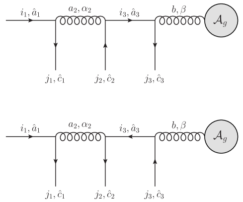
Let us consider a scattering process with $n$ external parton legs, carrying hard momenta $\{p_{i}\}$. Each external line $i$ will carry an index $A_{i}$ in the flavour/spin space that has been introduced above. Following Fig. 8 (c.f. Fig 5), we label the amplitude with external wavefunctions removed as ${\cal A}^{\bar{A}_{1}\ldots\bar{A}_{n}}_{A_{1}\ldots A_{n}}$, where barred indices are colour indices as before. The full hard-scattering amplitude then takes the form

$${\cal A}(\{p_{i}\})={\cal A}^{\bar{A}_{1}\ldots\bar{A}_{n}}_{A_{1}\ldots A_{n}}(\{p_{i}\})\prod_{i=1}^{n}\xi^{\bar{A}_{i}}_{A_{i}}(p_{i})\,,$$ (3.30)

where we again use $\xi^{\bar{A}}_{A}$ to denote the external wave function for a particle with species index $A$ and colour index $\bar{A}$. We may then describe the emission of any number of virtual soft partons from the external lines by dressing each line of the stripped amplitude with the generalised soft-emission operator of Eq. (3.24), such that this is sandwiched between the amplitude and the external wavefunctions. That is, we may define a generalised (and flavour-changing) soft function

$${\cal A}(\{p_{i}\})=\left(\prod_{i=1}^{n}\xi^{\bar{A}_{i}}_{A_{i}}(p_{i})\right){\cal S}^{\bar{A}_{1}\ldots\bar{A}_{n},\bar{B}_{1}\ldots\bar{B}_{n}}_{A_{1}\ldots A_{n},B_{1}\ldots B_{n}}\,{\cal A}^{\bar{B}_{1}\ldots\bar{B}_{n}}_{B_{1}\ldots B_{n}}\,,$$ (3.31)

where now ${\cal A}$ is the full amplitude dressed by soft parton emission, and the generalised soft function is given by

$${\cal S}^{\bar{A}_{1}\ldots\bar{A}_{n},\bar{B}_{1}\ldots\bar{B}_{n}}_{A_{1}\ldots A_{n},B_{1}\ldots B_{n}}=\Big{\langle}0\Big{|}\prod_{i=1}^{n}{\cal F}^{\bar{A}_{i}\bar{B}_{i}}_{A_{i}B_{i}}(p_{i})\Big{|}0\Big{\rangle}\,.$$ (3.32)

That is, the soft function is defined similarly to the pure gluon emission case, by a VEV of generalised soft-emission operators acting along each incoming particle contour. We may note that it is matrix-valued in the tensor product space of the flavour/spin and colour indices associated with each hard line. Note that this is directly analogous to how the usual soft function is matrix-valued in the tensor product space of colour indices, so the definition in Eq. (3.32) presents no significant additional complication from the conceptual point of view. As in Eq. (2.5), we may write a path-integral formula for the definition of Eq. (3.32). Let us first introduce the compact notation

$${\cal D}\Theta^{\bar{C}}_{C}\equiv{\cal D}\psi^{i}\,{\cal D}\bar{\psi}^{j}\,{\cal D}A_{\mu}^{a}\,,$$ (3.33)

i.e. the path-integral over the individual parton fields appearing in Eq. (3.8) can be simply written as a single measure involving the array of fields $\Theta_{C}^{\bar{C}}$. Then Eq. (3.32) may be written as

$${\cal S}_{A_{1}\ldots A_{n},B_{1}\ldots B_{n}}^{\bar{A}_{1}\ldots\bar{A}_{n},\bar{B}_{1}\ldots\bar{B}_{n}}=\int{\cal D}\Theta^{\bar{C}}_{C}\,\left(\prod_{i=1}^{n}{\cal F}^{\bar{A}_{i}\bar{B}_{i}}_{A_{i}B_{i}}(p_{i})\right)e^{iS[\Theta^{\bar{C}}_{C}]}\,,$$ (3.34)

which is similar in form to the pure gluon case of Eq. (2.5), and

$\displaystyle S[\Theta^{\bar{C}}_{C}]=\int{\rm d}^{d}x\,\mathcal{L}_{\rm QCD}\,$ (3.35)

is the QCD action. Consequently, the replica trick argument for exponentiation of arbitrary soft parton corrections proceeds by direct analogy to the soft gluon case. Carrying out the path integral over the compound soft parton field $\Theta^{\bar{C}}_{C}$ generates all possible Feynman diagrams in which the external hard partons are connected by soft partons. We may then introduce $N$ identical replicas of the original soft parton field, such that Eq. (2.9) is replaced by

$\displaystyle\left[{\cal S}_{N}\right]_{A_{1}\ldots A_{n},B_{1}\ldots B_{n}}^{\bar{A}_{1}\ldots\bar{A}_{n},\bar{B}_{1}\ldots\bar{B}_{n}}$ $\displaystyle=\int{\cal D}[\Theta^{(1)}]^{\bar{C}}_{C}\ldots{\cal D}[\Theta^{(n)}]^{\bar{C}}_{C}\,\exp\left\{i\sum_{j=1}^{N}S\Big{[}[\Theta^{(j)}]^{\bar{C}}_{C}\Big{]}\right\}$ (3.36)
$\displaystyle\quad\times\,\prod_{k=1}^{n}{\cal R}\left\{{\cal P}\exp\left(ig_{s}{\bf T}^{\bar{C}}\,\sum_{j=1}^{N}\int{\rm d}t_{k}\,{\bf Q}^{C}[\Theta^{(j)}]^{\bar{C}}_{C}(t_{k}p_{k})\right)\right\}^{\bar{A}_{i}\bar{B}_{i}}_{A_{i}B_{i}}.$

There is now a product of generalised soft-emission operators on each external leg, associated with the different soft parton replicas that may be emitted. As before, there is a replica-ordering operator, which in any given diagram acts to reorder parton emissions as necessary. We must bear in mind, however, that the action of the replica-ordering operator ${\cal R}$ in Eq. (3.36) is more complicated than for pure soft gluon emission. In the present case, the replica-ordering operator acts on the full transition matrix $[{\cal T}_{IJ}]_{C,AB}^{\bar{C},\bar{A}\bar{B}}$, instead of only on the colour matrices as was the case for soft-gluon emissions. This leads us to introduce $[{\cal T}_{N,IJ}(D)]_{C,AB}^{\bar{C},\bar{A}\bar{B}}$, which is the transition matrix of a replicated theory. This matrix will determine both the colour factor and the kinematic numerator of a given diagram, whereas the denominator is untouched. To see this, let us decompose the kinematic part of a given soft diagram $D$ in momentum space as

$${\cal K}(D)=\frac{{\cal N}(D)}{{\cal D}(D)}\,,$$ (3.37)

where ${\cal N}(D)$ is a kinematic numerator factor, which results from combining the emission factors $\{Q^{C,AB}\}$ of the transition functions for each emitted soft parton, as well as coupling factors, external wavefunctions etc. The denominator ${\cal D}$ arises from performing the integrals over the distance parameters $\{t_{k}\}$, which results in a product of nested momentum factors as exemplified in Eq. (3.26). While the numerator depends on the spinor structure of the diagrams, the denominator only depends on the kinematic assignment. If only soft gluons are emitted, the kinematic numerator for a diagram $D$ with $n_{j}$ soft emissions on a given line $j$ takes the simple form

$${\cal N}(D)\propto\prod_{j}p^{\mu_{1}}p^{\mu_{2}}\ldots p^{\mu_{j}}\,.$$

That is, there is a simple factor of the hard momentum for each emission, such that the emission factors for individual emissions commute with each other, and the numerator for any diagram with the same number of emissions on each line is the same. This indeed follows straightforwardly from the conventional Wilson line definition of Eq. (2.4), where the only non-commuting quantity in the exponent is the colour generator ${\bf T}_{i}$, and it is for this reason that the replica ordering operator ${\cal R}$ acts to modify the colour factors of graphs $C(D)\rightarrow\tilde{C}(D)$, but not their kinematics. This ceases to be the case for the generalised soft emission operator of Eq. (3.24). In this case the emission factors are not mutually commuting, and so the action of ${\cal R}$ is to reorder them, in addition to the colour generators. In the replicated theory, we denote by ${\cal N}_{N}(D)$ the kinematic numerator of diagram $D$, such that its full contribution is

$$C_{N}(D)\,{\cal K}_{N}(D)=\frac{{\cal N}_{N}(D)\,C_{N}(D)}{{\cal D}(D)}\,,$$ (3.38)

where the replicated colour factor $C_{N}(D)$ is defined as in the case of pure gluon emission. Despite this additional complication, the replica trick argument proceeds as before, where the logarithm of the soft amplitude can be directly obtained by taking the ${\cal O}(N)$ part of each soft diagram. Defining exponentiated numerators and colour factors via

$$\tilde{{\cal N}}(D)={\cal N}_{N}(D)\Big{|}_{{\cal O}(N)}\,,\quad\tilde{C}(D)=C_{N}(D)\Big{|}_{{\cal O}(N)}\,,$$ (3.39)

we may write the contribution of a given soft diagram to the logarithm of the amplitude as

$$\tilde{E}(D)=\frac{\tilde{\cal N}(D)\,\tilde{C}(D)}{{\cal D}(D)}\,.$$ (3.40)

An exponentiated form of the soft function is then simply found as

$\displaystyle\mathcal{S}={\rm exp}\left[\sum_{D}\tilde{E}(D)\right],$ (3.41)

where $\tilde{E}(D)$ are the generalised webs.

Refer to caption
Figure 9: Diagrams (a) and (b) constitute a generalization at NLP of the web in Fig. 3.

As in the pure gluon emission case, the replica trick provides a completely systematic way of calculating the logarithm of the soft amplitude directly, rather than the amplitude itself. However, the abstract nature of the generalised soft function of Eq. (3.36), and the exponentiated numerators appearing in Eq. (3.40), will doubtless look rather baffling to the reader. To explain our notation, let us consider an example. We take an amplitude with external partons $q(p_{1})$ and $\bar{q}(p_{2})$, which define two hard outgoing legs. At one-loop level, these fermions can either remain the same flavour (LP), or transition into gluons (NLP). When allowing for two loops, we may either consider two gluon exchanges (LP), one gluon and one fermion exchange (NLP), or two fermionic exchanges (NNLP). For this example we focus on the NLP contribution to the two-loop diagram, meaning that the external particles will have to be gluons. We thus consider two insertions of the replicated transition matrix on each leg, as shown in Fig. 9. For diagram (a) we denote the ordering of transition matrices as

$\displaystyle\left[{\cal T}^{(i)}(p_{1})\right]^{\bar{C}_{1},\bar{A}_{1}\bar{a}_{1}}_{C_{1},A_{1}a_{1}}\left[{\cal T}^{(j)}(p_{1})\right]^{\bar{C}_{2},\bar{a}_{1}\bar{B}_{1}}_{C_{2},a_{1}B_{1}}\left[{\cal T}^{(i)}(p_{2})\right]^{\bar{C}_{1},\bar{A}_{2}\bar{a}_{2}}_{C_{1},A_{2}a_{2}}\left[{\cal T}^{(j)}(p_{2})\right]^{\bar{C}_{2},\bar{a}_{2}\bar{B}_{2}}_{C_{2},a_{2}B_{2}}\,.$ (3.42)

This object is sandwiched in between two external wave functions $\epsilon^{\dagger}_{B_{1}}(p_{1})$ and $\epsilon^{\dagger}_{B_{2}}(p_{2})$, and a hard-scattering matrix $\mathcal{A}(p_{1},p_{2})_{A_{1}A_{2}}^{\bar{A}_{1}\bar{A}_{2}}$. In Eq. (3.42), lower-case letters correspond to intermediate particles on the hard lines. The replica-reordering operator leaves the order the same for all choices of $i,j$. This is not true for diagram (b), for which the ordering of transition matrices is

$\displaystyle{\cal T}^{(i)}(p_{1}){\cal T}^{(j)}(p_{1}){\cal T}^{(j)}(p_{2}){\cal T}^{(i)}(p_{2})\,.$ (3.43)

Here we leave the indices implicit for ease of notation. The reordering acts as follows:

$\displaystyle{\cal R}\left[{\cal T}^{(i)}(p_{1}){\cal T}^{(j)}(p_{1}){\cal T}^{(j)}(p_{2}){\cal T}^{(i)}(p_{2})\right]=\begin{cases}{\cal T}^{(i)}(p_{1}){\cal T}^{(j)}(p_{1}){\cal T}^{(i)}(p_{2}){\cal T}^{(j)}(p_{2})&\,i<j\quad\left(\frac{N(N-1)}{2}\right),\\ {\cal T}^{(j)}(p_{1}){\cal T}^{(i)}(p_{1}){\cal T}^{(j)}(p_{2}){\cal T}^{(i)}(p_{2})&\,j<i\quad\left(\frac{N(N-1)}{2}\right),\\ {\cal T}^{(j)}(p_{1}){\cal T}^{(j)}(p_{1}){\cal T}^{(j)}(p_{2}){\cal T}^{(i)}(p_{2})&\,i=j\quad(N)\,,\\ \end{cases}$ (3.44)

where we have also denoted the multiplicity of each replica assignment in the round brackets. In direct analogy with the soft-gluon case, we see that the first two expressions correspond to the ordering for diagram (a), whereas the last entry is the ordering for diagram (b). When combined with the external wave functions, we can write the contribution of diagram (b) to the logarithm of the generalised soft function as

$\displaystyle\widetilde{E}(b)=\frac{{\cal N}(b)C(b)-{\cal N}(a)C(a)}{{\cal D}(b)}\,.$ (3.45)

The projection onto external wave functions and the hard-scattering amplitude will turn the matrix notation into a sum expression, and will contract the open indices of the transition matrices.

So far we have discussed the use of the replica trick for virtual corrections only. Let us now generalise this to include real emissions.

3.4 The replica trick for real emissions

The starting point for using the replica trick in the case of virtual exchanges is to consider a generating functional for virtual soft parton diagrams (Eq. (3.34) in the general case). In the replicated theory, the corresponding functional is simply given by the original one raised to a power, as in Eq. (2.6). It is this fact that allows one to conclude that the ${\cal O}(N)$ contribution to diagrams in the replicated theory formally exponentiates. To include real emissions, we must therefore identify a suitable generating functional, such that the appropriate analogue of Eq. (2.6) can be applied. To this end, we simplify our arguments for the moment by considering a toy model of a single scalar field $\phi$, and a generating functional of the form

$$Z=\int{\cal D}\phi\,\Psi[\phi]e^{iS[\phi]}\,,$$ (3.46)

where $\Psi[\phi]$ is some function of the field that is the analogue of the product of generalised soft emission operators in Eq. (3.34). As is well-known, functionals such as those of Eqs. (3.34, 3.46) generate all possible Green’s functions, or vacuum expectation values of (time-ordered) products of fields. Usually in scalar field theory, one introduces a current $J$ conjugate to $\phi$, such that differentiation with respect to this current can be used to pick out Green’s functions of arbitrary multiplicity. Here, we will instead use the alternative approach of Ref. [147]. First, we may separate the action into its free-field part and an interaction term

$$S=S_{0}+S_{I}=\int{\rm d}^{d}x\,\left(\frac{1}{2}\phi K\phi+S_{I}\right)\,.$$ (3.47)

Here $K$ is the operator appearing in the quadratic term in the Lagrangian. To carry out the path integral, one may use the integral identity

$$\int{\rm d}u\,e^{-uMu/2}f(u+v)\,\sim\,e^{\partial_{v}M^{-1}\partial_{v}/2}f(v)\,,$$ (3.48)

where we have neglected an overall factor. By applying the appropriate functional generalisation of this around $v=0$, the path integral in Eq. (3.46) can be carried out (after substituting Eq. (3.47)) to give

$$Z=\left.\exp\left[-\int{\rm d}^{d}x\,{\rm d}^{d}x^{\prime}\,\frac{1}{2}\frac{\delta}{\delta\phi(x)}\Delta(x-x^{\prime})\frac{\delta}{\delta\phi(x^{\prime})}\right]e^{iS_{I}[\phi]}\Psi[\phi]\right|_{\phi=0}\,.$$ (3.49)

Here $\Delta(x-x^{\prime})$ is the Feynman propagator, corresponding (up to a numerical factor) with the inverse of the operator $K$. This is a less standard form of the generating functional, but nevertheless generates the usual Feynman diagram expansion. To see this, note that Taylor expanding the factors on the right-hand side yields a sum of products of the field $\phi$, where these come manifestly from interaction vertices of the theory. The latter may be contained in the interaction Lagrangian appearing in $S_{I}$, or the function $\Psi[\phi]$. In the case of soft parton emission, this corresponds to vertices off or on the hard particle lines respectively. The prefactor in Eq. (3.49) takes pairs of fields appearing in each term, and strips them off in favour of a propagator. After setting $\phi\rightarrow 0$, one is left with a sum of contributions in which interaction vertices are joined by propagators. These are the usual Feynman diagrams, and the exponential dependence in the prefactor turns out to be precisely such as to yield the required combinatorial factors associated with the usual Feynman rules. Examples can be found in Ref. [147] for conventional scalar field theory, although we have here modified the argument slightly so that it provides a scalar analogue of Eq. (3.34). All Feynman diagrams will then correspond to hard particle lines which are connected by conventional propagators and interaction vertices. That is, Eq. (3.49) generates virtual diagrams only, as expected from the fact that the original generating function of Eq. (3.49) is a vacuum-to-vacuum transition amplitude.

So much for virtual corrections. Next, we can include the effect of real corrections, and before doing so we note that the exponential prefactor appearing in Eq. (3.49) can be written in momentum space as [147]

$$\exp\left[-\int{\rm d}^{d}x\,{\rm d}^{d}x^{\prime}\,\frac{1}{2}\frac{\delta}{\delta\phi(x)}\Delta(x-x^{\prime})\frac{\delta}{\delta\phi(x^{\prime})}\right]=\exp\left[\int\frac{{\rm d}^{d}p}{(2\pi)^{d}}\frac{1}{2}\frac{\delta}{\delta\phi(p)}\Delta(p)\frac{\delta}{\delta\phi(-p)}\right],$$ (3.50)

where we have used the same symbol for the field and propagator in position or momentum space, but where the argument resolves any ambiguity. To include real corrections, we may consider the cut propagator

$$\Delta_{+}(p)=2\pi\Theta(p^{0})\delta\left[(p^{2}+m^{2})\right].$$ (3.51)

Then, a generating functional for the squared amplitude is

$$Z_{\rm sq}=Z\exp\left[-\int\frac{{\rm d}^{d}p}{(2\pi)^{d}}\frac{1}{2}\frac{\overleftarrow{\delta}}{\delta\phi(p)}\Delta_{+}(p)\frac{\overrightarrow{\delta}}{\phi(-p)}\right]Z^{\dagger}.$$ (3.52)

Here the arrows on the derivatives indicate that they act to the left or right, and we have introduced the generating functionals for virtual diagrams $Z$ and $Z^{\dagger}$ on either side of the final-state cut. By direct analogy with Eqs. (3.49, 3.50), the factor in the middle acts to strip off pairs of fields, and replace them with a propagator. Now, however, this is a cut propagator, and connects fields on different sides of the cut, as is required for a real particle. We have here considered the simplified case of a scalar field to simplify our arguments. However, it is straightforward to generalise this to the soft parton case. Let ${\cal S}$ be the (virtual) soft function of Eq. (3.34) with colour and species indices suppressed. A suitable generating functional for the squared amplitude is

$$Z_{{\rm sq}}={\cal S}\exp\left[-\int\frac{{\rm d}^{d}p}{(2\pi)^{d}}\frac{1}{2}\frac{\overleftarrow{\delta}}{\delta\Theta^{\bar{C}}_{C}(p)}\Delta_{+\phantom{,}CD}^{\phantom{+,}\bar{C}\bar{D}}(p)\frac{\overrightarrow{\delta}}{\delta\bar{\Theta}^{\bar{D}}_{D}(-p)}\right]{\cal S}^{\dagger},$$ (3.53)

where we have been careful to note that the functional differentiation acting to the right involves the conjugate field to that acting to the left.777 The Keldysh formalism [148, 149] provides provide an alternative approach to arrive at an equivalent form of Eq. (3.53) (also see Appendix C of Ref. [150] for an application to the Drell-Yan Soft function).

We can now apply the replica trick. Upon replicating the soft parton theory, Eq. (3.53) is replaced by

$$Z_{{\rm sq},N}={\cal S}_{N}\left\{\prod_{i=1}^{N}\exp\left[-\int\frac{d^{d}p}{(2\pi)^{d}}\frac{1}{2}\frac{\overleftarrow{\delta}}{\delta\Theta^{(i)\bar{C}}_{C}(p)}\Delta_{+\phantom{,}CD}^{\phantom{+,}\bar{C}\bar{D}}(p)\frac{\overrightarrow{\delta}}{\delta\bar{\Theta}^{(i)\bar{D}}_{D}(-p)}\right]\right\}{\cal S}^{\dagger}_{N},$$ (3.54)

where $\Theta_{C}^{(i)\bar{C}}$ is the compound soft parton field associated with replica $i$. Furthermore, we have introduced the replicated generating functional for virtual soft-parton exchange diagrams of Eq. (3.36), again with colour and flavour indices suppressed. Given that this functional satisfies ${\cal S}_{N}={\cal S}^{N}$, we obtain

$$Z_{{\rm sq},N}=(Z_{\rm sq})^{N}=1+N\log(Z_{\rm sq})+{\cal O}(N^{2})\,.$$ (3.55)

Thus, the usual replica trick arguments apply,888In extending this statement to a given observable, one must make sure that the corresponding measurement function does not differentiate between the exchanged soft partons. This will indeed be the case for infrared-safe observables. and the ${\cal O}(N)$ piece of an arbitrary diagram contributes to the logarithm of the squared soft parton amplitude. This succeeds in proving the exponentiation of either real or virtual soft parton corrections, as well as providing a systematic method for deriving how the colour and/or kinematic dependence of Feynman diagrams becomes modified upon their entering the logarithm of the soft function. In the following sections, we illustrate the use of the abstract arguments of this and the preceding sections, by applying them to processes of phenomenological interest.

4 Real emission corrections in DIS

Refer to caption
Figure 10: Squared Feynman diagram for the DIS process at LO.

As a testing ground for applying the replica trick to the generalised soft function, we will consider photon-initiated deep-inelastic scattering (DIS) process. This serves two purposes: we will reproduce a known exponentiation property of soft quark and gluon emissions, which was recently used in Ref. [123] (see also Ref. [117]) to resum NLP logarithms in the off-diagonal DGLAP splitting functions. Secondly, the discussion in this section paves the way for the proof (in the following section) of a conjecture made in Refs. [117, 113], namely that the leading virtual corrections in the quark channel should formally exponentiate.

First we introduce some notation. At LO, the incoming virtual photon couples to a valence quark, leading to the process

$$q(p)+\gamma^{*}(q)=q(p_{2})\,,$$ (4.1)

The LO squared Feynman diagram is shown in Fig. 10, and it is conventional to define

$$Q^{2}=-q^{2}>0\,,\qquad\qquad x=\frac{Q^{2}}{2\,p\cdot q}\,,$$ (4.2)

where the latter is the so-called Björken $x$ variable. In terms of these parameters, one may define the structure function

$$F_{2}(x,Q^{2})=\int{\rm d}\Phi_{1}\,T_{2}^{\alpha\beta}\,\overline{|{\cal A}|^{2}_{\alpha\beta}}\,,$$ (4.3)

with ${\rm d}\Phi_{1}$ the one-particle phase-space. The integrand contains the squared amplitude summed (averaged) over final (initial) colours and spins respectively, with photon Lorentz indices as in Fig. 10. We have also introduced the projector

$$T_{2}^{\alpha\beta}=-\frac{1}{4\pi}\frac{1}{1-\epsilon}\left(\eta^{\alpha\beta}+(3-2\epsilon)\frac{q^{2}}{(p\cdot q)^{2}}p^{\alpha}p^{\beta}\right),$$ (4.4)

where we work in $d=4-2\epsilon$ dimensions. The LO amplitude and complex conjugate amplitude read

$\displaystyle\big{[}\mathcal{A}^{(0)}\big{]}^{\alpha}$ $\displaystyle=\bar{u}_{\hat{b}}^{j}(p_{2})\,ie\gamma_{\hat{b}\hat{a}}^{\alpha}\delta^{ji}\,u_{\hat{a}}^{i}(p_{2}),$ (4.5a)
$\displaystyle\big{[}\mathcal{A}^{{\dagger}(0)}\big{]}^{\beta}$ $\displaystyle=\bar{u}_{\hat{a}^{\prime}}^{i^{\prime}}(p)\,(-i)e\gamma_{\hat{a}^{\prime}\hat{b}^{\prime}}^{\beta}\delta^{i^{\prime}j^{\prime}}\,u_{\hat{b}^{\prime}}^{j^{\prime}}(p_{2}),$ (4.5b)

leading to

$$\overline{|{\cal A}^{(0)}|^{2}_{\alpha\beta}}=\frac{e^{2}}{2}{\rm Tr}\big{[}\not{p}\gamma_{\beta}\not{p}_{2}\gamma_{\alpha}\big{]}.$$ (4.6)

The matrix element squared is then inserted in Eq. (4.3), where at LO one has

$$\int{\rm d}\Phi_{1}=\int\frac{{\rm d}^{d}p_{2}}{(2\pi)^{d-1}}\,(2\pi)^{d}\delta^{(d)}(p+q-p_{2})\,\delta(p_{2}^{2})\theta(p_{2}^{0})=\frac{2\pi}{Q^{2}}\delta(1-x)\theta(Q).$$ (4.7)

With the normalization given by the projector in Eq. (4.4), one easily finds

$$F^{(0)}_{2}(x,Q^{2})=\delta(1-x),$$ (4.8)

where the superscript (0) indicates that this is the leading order (Born) result.

At higher orders the emission of soft particles can be expressed in terms of the generalised soft emission operators introduced in Section 3.2. To this end, let us define the vector of amplitudes with stripped-off spinors/polarisation vectors:

$$\big{[}\mathcal{A}^{(0)}_{\alpha}\big{]}^{\bar{B}\bar{A}}_{BA}=\left([\mathcal{A}^{(0)}_{q,\alpha}]^{ji}_{\hat{b}\hat{a}},0,0\right),\qquad\qquad\big{[}\mathcal{A}^{{\dagger}(0)}_{\beta}\big{]}^{\bar{A}^{\prime}\bar{B}^{\prime}}_{A^{\prime}B^{\prime}}=\left([\mathcal{A}^{{\dagger}(0)}_{q,\beta}]^{i^{\prime}j^{\prime}}_{\hat{a}^{\prime}\hat{b}^{\prime}},0,0\right).$$ (4.9)

The stripped-off amplitudes can be obtained by direct comparison with (4.5), and we obtain

$$\big{[}\mathcal{A}_{q}^{(0)\alpha}\big{]}^{ji}_{\hat{b}\hat{a}}=ie\gamma_{\hat{b}\hat{a}}^{\alpha}\delta^{ji},\qquad\qquad\big{[}\mathcal{A}_{q}^{{\dagger}(0)\beta}\big{]}^{i^{\prime}j^{\prime}}_{\hat{a}^{\prime}\hat{b}^{\prime}}=-ie\gamma_{\hat{a}^{\prime}\hat{b}^{\prime}}^{\beta}\delta^{i^{\prime}j^{\prime}}.$$ (4.10)

In this notation, the tree level matrix element squared reads

$\displaystyle\overline{|{\cal A}^{(0)}|^{2}_{\alpha\beta}}$ $\displaystyle=$ $\displaystyle\frac{1}{2N_{c}}\bar{\xi}^{\bar{A}^{\prime}}_{A^{\prime}}(p)\big{[}\mathcal{A}^{{\dagger}(0)\beta}\big{]}^{\bar{A}^{\prime}\bar{B}^{\prime}}_{A^{\prime}B^{\prime}}\xi^{\bar{B}^{\prime}}_{B^{\prime}}(p_{2})\,\bar{\xi}^{\bar{B}}_{B}(p_{2})\big{[}\mathcal{A}^{(0)\alpha}\big{]}^{\bar{B}\bar{A}}_{BA}\xi^{\bar{A}}_{A}(p)\,,$

where the vector of spinors/polarisation vectors in the first line has been defined in Eqs. (3.9), (3.16), and we use the summation convention for repeated species indices. Inserting the expressions from (4.10) in the second line above one readily reproduces Eq. (4.6).

The hard-scattering amplitude may now be dressed with emissions of soft particles through adding generalised soft emission operators:

$\displaystyle\overline{|{\cal A}|^{2}_{\alpha\beta}}$ $\displaystyle=$ $\displaystyle\sum_{m}\frac{1}{{\cal N}_{s}{\cal N}_{c}}\left\langle 0\left|\Big{(}\bar{\xi}^{\bar{A}_{1}^{\prime}}_{A_{1}^{\prime}}(p)\,\big{[}{\cal F}_{1,\rm out}^{{\dagger}}\big{]}^{\bar{A}^{\prime}_{1}\bar{A}^{\prime}_{2}}_{A^{\prime}_{1}A^{\prime}_{2}}\,\big{[}\mathcal{A}^{{\dagger}(0)\beta}\big{]}^{\bar{A}_{2}^{\prime}\bar{B}_{2}^{\prime}}_{A_{2}^{\prime}B_{2}^{\prime}}\,\big{[}{\cal F}_{2,\rm in}\big{]}^{\bar{B}^{\prime}_{2}\bar{B}^{\prime}_{1}}_{B^{\prime}_{2}B^{\prime}_{1}}\,\xi^{\bar{B}^{\prime}_{1}}_{B^{\prime}_{1}}(p_{2})\Big{)}\right|m\right\rangle$ (4.11)
$\displaystyle\hskip 42.67912pt\times\,\left\langle m\left|\Big{(}\bar{\xi}^{\bar{B}_{1}}_{B_{1}}(p_{2})\,\big{[}{\cal F}_{2,\rm out}^{{\dagger}}\big{]}^{\bar{B}_{1}\bar{B}_{2}}_{B_{1}B_{2}}\,\big{[}\mathcal{A}^{(0)\alpha}\big{]}^{\bar{B}_{2}\bar{A}_{2}}_{B_{2}A_{2}}\,\big{[}{\cal F}_{1,\rm in}\big{]}^{\bar{A}_{2}\bar{A}_{1}}_{A_{2}A_{1}}\,\xi^{\bar{A}_{1}}_{A_{1}}(p)\Big{)}\right|0\right\rangle,$

where the factors ${\cal N}_{s}$, ${\cal N}_{c}$ represent the spin and color average over the initial-state particle. At tree level the initial state particle is a quark, thus ${\cal N}_{s_{q}}=2$, ${\cal N}_{c_{q}}=N_{c}$, as in Eq. (4). At higher orders it is possible to have gluons in the initial state, leading to ${\cal N}_{s_{g}}=(d-2)$, ${\cal N}_{c_{g}}=N_{c}^{2}-1$. Introducing a soft function with $m$ real gluon emissions:

$$\big{(}{\cal S}_{m}\big{)}^{\bar{A}^{\prime}_{1}\bar{A}^{\prime}_{2}\,\bar{B}^{\prime}_{2}\bar{B}^{\prime}_{1}\,\bar{B}_{1}\bar{B}_{2}\,\bar{A}_{2}\bar{A}_{1}}_{A^{\prime}_{1}A^{\prime}_{2}\,B^{\prime}_{2}B^{\prime}_{1}\,B_{1}B_{2}\,A_{2}A_{1}}=\left\langle 0\left|\big{[}{\cal F}_{1,\rm out}^{{\dagger}}\big{]}^{\bar{A}^{\prime}_{1}\bar{A}^{\prime}_{2}}_{A^{\prime}_{1}A^{\prime}_{2}}\,\big{[}{\cal F}_{2,\rm in}\big{]}^{\bar{B}^{\prime}_{2}\bar{B}^{\prime}_{1}}_{B^{\prime}_{2}B^{\prime}_{1}}\right|m\right\rangle\left\langle m\left|\big{[}{\cal F}_{2,\rm out}^{{\dagger}}\big{]}^{\bar{B}_{1}\bar{B}_{2}}_{B_{1}B_{2}}\,\big{[}{\cal F}_{1,\rm in}\big{]}^{\bar{A}_{2}\bar{A}_{1}}_{A_{2}A_{1}}\right|0\right\rangle,$$ (4.12)

we can write Eq. (4.11) as

$\displaystyle\overline{|{\cal A}|^{2}_{\alpha\beta}}$ $\displaystyle=$ $\displaystyle\frac{1}{{\cal N}_{s}{\cal N}_{c}}\sum_{m}\,\Big{(}\bar{\xi}^{\bar{A}_{1}^{\prime}}_{A_{1}^{\prime}}(p)\,\big{[}\mathcal{A}^{{\dagger}(0)\beta}\big{]}^{\bar{A}_{2}^{\prime}\bar{B}_{2}^{\prime}}_{A_{2}^{\prime}B_{2}^{\prime}}\,\xi^{\bar{B}^{\prime}_{1}}_{B^{\prime}_{1}}(p_{2})\Big{)}$ (4.13)
$\displaystyle\hskip 56.9055pt\times\,\big{(}{\cal S}_{m}\big{)}^{\bar{A}^{\prime}_{1}\bar{A}^{\prime}_{2}\,\bar{B}^{\prime}_{2}\bar{B}^{\prime}_{1}\,\bar{B}_{1}\bar{B}_{2}\,\bar{A}_{2}\bar{A}_{1}}_{A^{\prime}_{1}A^{\prime}_{2}\,B^{\prime}_{2}B^{\prime}_{1}\,B_{1}B_{2}\,A_{2}A_{1}}\,\Big{(}\bar{\xi}^{\bar{B}_{2}}_{B_{2}}(p_{2})\,\big{[}\mathcal{A}^{(0)\alpha}\big{]}^{\bar{B_{2}}\bar{A}_{2}}_{B_{2}A_{2}}\,\xi^{\bar{A}_{1}}_{A_{1}}(p)\Big{)}.$

Upon inserting this into Eq. (4.3) and performing the relevant phase-space integrals, one obtains the LL result for the structure function at any power. Let us stress that the above amplitude only should reproduces the maximally soft momentum configuration, i.e. the LL contribution. Corrections beyond LL could in principle be taken into account by modifying the diagonal terms ${\cal T}_{ii}^{\rm in}(p)$ of the transition matrix in Eq. (3.13), with $i=q$, $\bar{q}$, $g$, in such a way to include NLP corrections to these transitions, but are not considered here.999They have been obtained in [125, 151], see in particular Eq. 5.7 of [151], which provide the NLP contribution to the diagonal terms of the generalised soft emission operator ${\cal F}$. In Appendix B we show explicitly how to calculate $F_{2}(x,Q^{2})$ at NLO, for which one needs to consider the diagrams in Figs. 11 and 12.

Refer to caption
Figure 11: Diagrams corresponding to the LP NLO soft function involving the exchange of a virtual (diagram a) or real (diagrams b, c, d) soft gluon. The corresponding soft function is given in Eq. (B.3), Eq. (B.4) and Eq. (B.3). The complex conjugate of diagrams (a) and (b) are not shown in this figure, but are taken into account in Eqs. (B.3) and (B.4).
Refer to caption
Figure 12: Diagrams corresponding to the NLP NLO soft function arising from the exchange of a soft (anti-)quark. The corresponding soft functions ${\cal S}_{\bar{q}}^{(1)}$ and ${\cal S}_{q}^{(1)}$ are given in Eq. (B.13) and (B.14) respectively. Notice that the label $\bar{q}$, $q$ refers to the particle that crosses the cut, not to the particle in the hard scattering amplitude ${\cal A}_{i}$, where the label is actually opposite compared to the label in the soft function. There are additional diagrams where the soft (anti-)quark is emitted from the line with momentum $p_{2}$. These however contribute beyond LL, as explained in the main text, and therefore are not shown here.

We now turn our attention to the exponentiation of the real emission diagrams by means of the replica trick. First of all, let us notice that the structure function $F_{2}$ is gauge invariant. We can exploit this by choosing a gauge where the calculation of higher-order contributions simplifies. To this end it proves useful [152, 153, 154] to consider physical gluon polarisation vectors defined via the requirements

$$k\cdot\epsilon(k)=c\cdot\epsilon(k)=0\,,$$ (4.14)

where $c$ is a null vector ($c^{2}=0$). This means that the sum over physical gluon polarisation states take the form

$${\cal P}_{\mu\nu}(k)=-\eta_{\mu\nu}+\frac{k_{\mu}c_{\nu}+k_{\nu}c_{\mu}}{c\cdot k}\,.$$ (4.15)

In what follows we consider

$$c=p_{2},$$ (4.16)

a choice which is particularly convenient, as it eliminates the need to consider ${\cal F}_{2}$ in the case of soft gluon emissions. For soft quark emissions, at NLP, ${\cal F}_{2}$ will contribute to at most NLL, which is also beyond what we are considering here. That is, we only need to take into account emissions from the generalised Wilson line ${\cal F}_{1,\rm in}$, ${\cal F}_{1,\rm out}^{{\dagger}}$. Indeed, it is easy to check that by setting $c=p_{2}$, only diagram (c) in Fig. 11 contributes to the real emission at LP, while diagrams (b) and (d) are zero.

Refer to caption
Figure 13: (a) Single soft topology corresponding to each of the partonic assignments in Figs. 11 (c) and 12 (a); (b) and (c) soft topologies generated at NNLO in the squared amplitude, with replica indices indicated.

With this, we note that the diagrams of Fig. 11(c) and Fig. 12(a), (b) are all given by the single topology in Fig. 13(a). At higher orders, using the gauge of Eq. (4.14), the LL of the real emission is given in terms of (crossed-)ladder diagrams, where emission of any partonic species is expressed by the transition matrix ${\cal T}_{IJ}$. In the case of DIS, at NNLO in the gauge defined by Eqs. (4.15) (4.16) one needs to take into account the two real topologies (b) and (c) in Fig. 13, namely an uncrossed and a crossed ladder, with replica index $i$ and $j$. One immediately sees that diagrams (b) and (c) of Fig. 13 are the analog of the diagrams in Fig. 9. Therefore, following the discussion in Section 3.3, the contributions of diagrams (b) and (c) to the logarithm of the generalised soft function in Eq. (3.41) read (Cf. Eq. (3.45))

$\displaystyle\widetilde{E}(b)=0,\qquad\qquad\widetilde{E}(c)=\frac{{\cal N}(c)C(c)-{\cal N}(b)C(b)}{{\cal D}(c)}\,.$ (4.17)

This result is consistent with exponentiation of the generalised soft-emission operator in the generalised soft function. To see this, let us explicitly construct the $\mathcal{O}(\alpha_{s}^{2})$ expansion of the soft function using the reduced diagrams of Eq. (4.17). With only one emission present, there is only one choice of replica index, and thus all graphs with one soft emission are ${\cal O}(N)$. They thus contribute to the logarithm of the soft function unmodified. When two partons are emitted, the only contribution that needs to be added according to Eq. (4.17) is $\widetilde{E}(c)$, the rest is already generated by the one-emission diagram. Therefore the logarithm of the soft function becomes

$$\ln{\cal S}=E(a)+\tilde{E}(c)\,,$$ (4.18)

where the first term corresponds to diagram (a) in Fig. 13. Focusing on the NNLO contribution, obtained after exponentiating the above result and then expanding $\cal S$ up to $\mathcal{O}(\alpha_{s}^{2})$, we obtain

$$\exp\left[\ln{\cal S}\right]\Big{|}_{\mathcal{O}(\alpha_{s}^{2})}=\frac{1}{2}\Big{[}E(a)\Big{]}^{2}+\frac{{\cal N}(c)C(c)-{\cal N}(b)C(b)}{{\cal D}(c)}\,.$$ (4.19)

In the first term, squaring the one-emission contribution will generate kinematic numerators, which are products of two distinct emissions on the left-and right-hand side of the cut. Selecting the correct partonic assignment will yield the kinematic numerator and colour factor of diagram (b). However, the denominator arising from squaring the one-emission graphs will have uncoupled momenta

$\displaystyle\Big{[}D(a)\Big{]}^{2}=(p\cdot k_{1})^{2}(p\cdot k_{2})^{2}\,,$ (4.20)

rather than the actual denominator of diagram (b), which is

$\displaystyle{\cal D}(b)=(p\cdot k_{1})^{2}[p\cdot(k_{1}+k_{2})]^{2}\,.$ (4.21)

The denominator for diagram (c) is

$\displaystyle{\cal D}(c)=(p\cdot k_{1})(p\cdot k_{2})[p\cdot(k_{1}+k_{2})]^{2}\,.$ (4.22)

Using the eikonal identity

$$\frac{1}{(p\cdot k_{1})[p\cdot(k_{1}+k_{2})]}+\frac{1}{(p\cdot k_{2})[p\cdot(k_{1}+k_{2})]}=\frac{1}{(p\cdot k_{1})}\frac{1}{(p\cdot k_{2})}\,,$$ (4.23)

we can write

$$\frac{1}{(p\cdot k_{1})^{2}(p\cdot k_{2})^{2}}=2\left[\frac{1}{{\cal D}(b)}+\frac{1}{{\cal D}(c)}\right],$$ (4.24)

where we have used the freedom to relabel $k_{1}\leftrightarrow k_{2}$ to identify $2{\cal D}(b)$, which is allowed given that all emission momenta are integrated over. We thus find

$$\frac{1}{2}\Big{[}E(a)\Big{]}^{2}={\cal N}(b)C(b)\left[\frac{1}{{\cal D}(b)}+\frac{1}{{\cal D}(c)}\right].$$ (4.25)

Combining this with the second term in Eq. (4.19) gives

$$\frac{1}{2}\Big{[}E(a)\Big{]}^{2}+\tilde{E}(c)=\frac{{\cal N}(b)C(b)}{{\cal D}(b)}+\frac{{\cal N}(c)C(c)}{{\cal D}(c)}\,.$$ (4.26)

That is, exponentiating the logarithm of the generalised soft function and extracting a given partonic assignment does indeed reproduce the conventional diagrams in the amplitude, with their correct kinematic numerators and colour factors. Similar arguments can be made at higher orders.

We now use the replica trick to obtain the LL contribution of the emission of a soft parton, in which case we need only consider the first term of $\ln\cal S$, namely the one consisting of a sum over all possible one real-emission contributions. In the gauge defined by Eq. (4.16), we may therefore simply exponentiate the NLO soft function $S^{(1)}$. The corresponding matrix element squared becomes

$\displaystyle\overline{|{\cal A}|^{2}_{\alpha\beta}}\big{|}_{\rm real}$ $\displaystyle=$ $\displaystyle\frac{1}{{\cal N}_{s}{\cal N}_{c}}\,\Big{(}\bar{\xi}^{\bar{A}_{1}^{\prime}}_{A_{1}^{\prime}}(p)\,\big{[}\mathcal{A}^{{\dagger}(0)\beta}\big{]}^{\bar{A}_{2}^{\prime}\bar{B}_{2}^{\prime}}_{A_{2}^{\prime}B_{2}^{\prime}}\,\xi^{\bar{B}^{\prime}_{1}}_{B^{\prime}_{1}}(p_{2})\Big{)}$ (4.27)
$\displaystyle\hskip 14.22636pt\times\,\exp\Big{[}{\cal S}^{(1)}\Big{]}^{\bar{A}^{\prime}_{1}\bar{A}^{\prime}_{2}\,\bar{B}^{\prime}_{2}\bar{B}^{\prime}_{1}\,\bar{B}_{1}\bar{B}_{2}\,\bar{A}_{2}\bar{A}_{1}}_{A^{\prime}_{1}A^{\prime}_{2}\,B^{\prime}_{2}B^{\prime}_{1}\,B_{1}B_{2}\,A_{2}A_{1}}\,\Big{(}\bar{\xi}^{\bar{B}_{2}}_{B_{2}}(p_{2})\,\big{[}\mathcal{A}^{(0)\alpha}\big{]}^{\bar{B_{2}}\bar{A}_{2}}_{B_{2}A_{2}}\,\xi^{\bar{A}_{1}}_{A_{1}}(p)\Big{)},$

Using this expression, we make contact with the known results at NLP for the quark-gluon channel in photon-induced DIS [123]. To this end, let us recall that expansion of the exponential in Eq. (4.27) generates contributions at all subleading power, but we can select the NLP term by associating a book-keeping parameter $\lambda\ll 1$ to the quark-gluon transitions in the matrix Eq. (3.13). The parameter $\lambda$ is chosen such that the soft momentum scales as $k\sim\lambda^{2}$, with $\lambda^{2}\sim(1-x)$ for $x\to 1$. Then it is easy to see that the LP and NLP soft functions scale respectively as $\lambda^{-4n}$ and $\lambda^{-4n+2}$ at order $\alpha_{s}^{n}$. To select the gluon-initiated DIS channel we need at least the exchange of a single soft fermion, which is suppressed by a power of $\lambda^{2}$ compared to the exchanged a soft gluon. Therefore, at ${\cal O}(\alpha_{s}^{n})$ the NLP contributions is obtained by allowing only one insertion of the soft function ${\cal S}_{\bar{g}q}$, $m$ insertions of ${\cal S}_{gg}$, and $n-1-m$ insertions of ${\cal S}_{qq}$. Given its length, the explicit expression is given in Eq. (B.17). Substituting the results for the partonic emission factors, contracting these with the LO amplitudes, and applying the eikonal identity as discussed e.g. in Sec 2.2.1 of [123] one finds for the squared NLP amplitude

$\displaystyle\overline{|{\cal A}|^{2}_{\alpha\beta}}\big{|}_{\rm qg,\,real,\,LL}^{(n)}$ $\displaystyle=\frac{g_{s}^{2n}\,e^{2}\,n_{f}\,T_{R}}{n!(d-2)}\left[\prod_{i=1}^{n-1}\frac{p^{\mu_{i}}p^{\nu_{i}}}{(p\cdot k_{i})^{2}}{\cal P}_{\mu_{i}\nu_{i}}(k_{i})\right]\sum_{m=0}^{n-1}C_{A}^{m}\,C_{F}^{n-1-m}$
$\displaystyle\quad\times\,\bigg{\{}{\rm Tr}\big{[}\not{k}_{q}\gamma^{\alpha_{1}^{\prime}}\not{p}\gamma_{\beta}\not{p}_{2}\gamma_{\alpha}\not{p}\gamma^{\alpha_{1}}\big{]}+{\rm Tr}\big{[}\not{k}_{q}\gamma^{\alpha_{1}}\not{p}\gamma_{\alpha}\not{p}_{2}\gamma_{\beta}\not{p}\gamma^{\alpha^{\prime}_{1}}\big{]}\bigg{\}}\frac{{\cal P}_{\alpha_{1}\alpha_{1}^{\prime}}(p)}{(2p\cdot k_{q})^{2}},$ (4.28)

This indeed agrees with the known form of the squared amplitude with one soft quark emission and $n-1$ soft gluon emissions, as conjectured in Ref. [142] and proven in Ref. [123].

As discussed above, in Eqs. (B.17), (4) we have only considered those graphs which are non zero in the gauge defined by Eqs. (4.15) and (4.16). One could of course choose a different gauge, in which case the remaining diagrams would have to be considered. These will exponentiate by the same arguments as above, leading the to same final (gauge-invariant) result.

Whilst the arguments of this section may take some getting used to, they greatly streamline the derivation of the all-order structure of the leading real emission corrections at arbitrary order in perturbation theory. That is, exponentiating the one-emission contribution to the generalised soft function leads immediately to the fact that at NLP, the soft quark emission process is dressed by $n-1$ soft gluons at ${\cal O}(\alpha_{s}^{n})$, where the emission momenta are uncoupled, and where there is a combinatorial factor of $1/n!$. The correct colour factor is also obtained, namely that associated with a sum over all possible uncrossed ladder graphs, in which gluons are emitted either before or after the soft quark emission.

To summarise, in this section we have used the structure of real emission corrections in DIS to illustrate the use of the replica trick in determining the leading singular behaviour of scattering amplitudes in the soft limit. As well as recovering previously proven results, however, we may also use the replica trick to prove a recent conjecture regarding virtual corrections in the same process. This is the subject of the following section.

5 Endpoint contributions in deep inelastic scattering

Ref. [117] considered the so-called off-diagonal splitting functions in deep-inelastic scattering, arising from kinematically subleading partonic channels that open up for the first time at NLO. The authors then derived the all-order structure of leading logarithmic terms, agreeing with the previous conjectures of Ref. [142]. However, in doing so, it was assumed that the leading IR divergent virtual corrections to each subleading partonic channel exponentiate. A related conjecture was made in Ref. [113], namely that leading virtual corrections to a certain form factor involving soft quark emission also exponentiate, and indeed this is the form factor that would replace the usual quark form form factor as applied to DIS, in generating subleading partonic emissions at NLO.

The aim of this section is to show how the above results naturally arise from using the replica trick arguments of this paper. To this end, we must again consider the generating functional for soft parton diagrams at the level of the squared amplitude, as constructed in Eq. (3.53). As explained after Eq. (3.54), this generating functional implies that the ${\cal O}(N)$ part of an arbitrary diagram enters the logarithm of the squared soft parton amplitude. However, to confirm the above conjecture, we must consider only those diagrams that have a single soft quark crossing the final state cut. This is straightforward using the generating functional of Eq. (3.54), but unfortunately does not lead directly to a proof (or otherwise) of the desired conjecture. To see why, it is sufficient to note that diagrams containing a single soft real quark will arise at any order in perturbation theory, such that some of them will indeed exponentiate. An example is shown in Fig. 14, and we can clearly add more soft gluons to this as desired. Thus, a naïve application of the replica trick results in a complicated form of the soft function for the squared amplitude, in which single soft quark corrections enter the logarithm at arbitrary orders. What the above conjecture then states is that it must somehow be possible to reorder the diagrammatic expansion, so that the soft quark emission factorises from the remaining soft gluon emissions, leading to a simple exponential form for the latter. Put more simply, the conjecture states that the additional soft gluon emissions dressing a single soft quark emission exponentiate. What is desirable is to isolate the single quark emission from the outset, such that the replica trick can be applied to the remaining soft gluon emissions alone.

Refer to caption
Figure 14: Example higher-order diagram with a single soft quark crossing the final state cut.

It is indeed possible to achieve this by appealing again to Eq. (3.53). The exponential operator in the middle of the diagram contracts pairs of (conjugate) fields on either side of the final state cut. If we are to have a single soft quark as the only real emission, then the exponential may be expanded to first-order only, retaining only the term involving the (anti-)quark fields. We may also simplify the generating functional ${\cal S}$ that appears on the left-hand side. This contains a generalised soft emission operator associated with each hard particle. However, only one soft quark emission needs to be included, from the incoming parton leg. On the latter, the operator of Eq. (3.24) takes the form

$${\cal P}\exp\left[ig_{s}\int{\rm d}t\left({\bf Q}_{\Psi}{\bf T}_{\Psi}\Psi(tp_{1})+{\bf Q}_{\bar{\Psi}}{\bf T}_{\bar{\Psi}}\bar{\Psi}(tp_{1})+{\bf T}^{a}p^{\mu}\sum_{i=1}^{N}A_{\mu}^{(i),a}(tp_{1})\right)\right],$$ (5.1)

where ${\bf Q}_{\Psi}$ (${\bf Q}_{\bar{\Psi}}$) and ${\bf T}_{\Psi}$ (${\bf T}_{\bar{\Psi}}$) are the kinematic and colour factors associated with soft (anti-)quark emission respectively. To NLP order, inclusion of a single soft quark emission amounts to expanding Eq. (5.1) to first order in ${\bf Q}_{\Psi}$, such that Eq. (5.1) becomes

$$\int_{-\infty}^{0}{\rm d}t_{q}\,\Phi_{1}(-\infty,t_{q})\left[{\bf Q}_{\Psi}{\bf T}_{\Psi}\Psi(t_{q}p)\right]\Phi_{1}(t_{q},0),$$ (5.2)

where $\Phi_{1}(a,b)$ is the conventional Wilson line operator on parton leg 1, between distance parameters $a$ and $b$. We have also introduced $t_{q}$ as the distance parameter at which the soft quark is emitted. All remaining soft emission operators in the squared amplitude can then be replaced with conventional Wilson lines, such that the generating functional for diagrams containing a single real soft quark emission becomes

$\displaystyle Z_{sq}\Big{|}_{q}$ $\displaystyle={\cal S}_{q}\left[-\int\frac{{\rm d}^{d}k_{q}}{(2\pi)^{d}}\frac{1}{2}\frac{\overleftarrow{\delta}}{\delta\Psi(k_{q})}\Delta^{(q)}_{+}(k_{q})\frac{\overrightarrow{\delta}}{\delta\bar{\Psi}(-k_{q})}\right]{\cal S}^{\dagger}_{q},$ (5.3)

where $\Delta^{(q)}_{+}$ is the appropriate cut propagator for a quark of momentum $k_{q}$, and we have introduced the generating functional for diagrams containing a single soft real quark:

$\displaystyle{\cal S}_{q}$ $\displaystyle=\int_{-\infty}^{0}{\rm d}t_{q}\int{\cal D}\Psi\int{\cal D}\bar{\Psi}\,{\bf Q}_{\Psi}{\bf T}_{\Psi}\Psi(t_{q}p_{1}){\cal S}_{A};$
$\displaystyle{\cal S}_{A}$ $\displaystyle=\left[\int{\cal D}A_{\mu}\Phi_{1}(-\infty,t_{q})\Phi_{1}(t_{q},0)\Phi_{2}(0,\infty)e^{iS[A_{\mu},\Psi,\bar{\Psi}]}\right].$ (5.4)

Here we have isolated the path integral over the soft gluon field, together with the Wilson lines that source the soft gluons.101010Although it appears that we may combine the two Wilson lines associated with the incoming parton leg with momentum $p_{1}$, it must be remembered that they contain colour matrices in different representations, due to acting on either side of the soft quark emission. This path integral acts to dress the amplitude for the emission of a single soft quark with additional gluon emissions, thus generating all possible virtual corrections to the single soft quark emission process. The soft gluons may interact either with the hard parton legs (through the Wilson lines), or with the emitted soft quark (via the interaction Lagrangian in the soft parton action). That these additional contributions exponentiate can now be surmised by replicating the soft gluon field $A_{\mu}$, but not the soft (anti-)quark fields. Then, in the replicated theory with $N$ replicas $A_{\mu}^{(i)}$, Eq. (5.4) becomes

$\displaystyle{\cal S}_{q,N}$ $\displaystyle=\int_{-\infty}^{0}{\rm d}t_{q}\int{\cal D}\Psi\int{\cal D}\bar{\Psi}\,{\bf Q}_{\Psi}{\bf T}_{\Psi}\Psi(t_{q}p_{1}){\cal S}_{A}^{N}.$ (5.5)

Following similar arguments to our previous cases, the ${\cal O}(N)$ piece of the soft gluon dressings exponentiates, precisely confirming the desired conjecture that virtual corrections to the soft quark emission process exponentiate.

For completeness, we mention a subtlety in the above argument. At higher orders, there will be diagrams in which fermion bubbles occur off the hard parton lines. These are generated by pulling down multiple interaction vertices from the action $S[A_{\mu},\Psi,\bar{\Psi}]$, and a potential problem occurs given that we have only replicated the soft gluons: gluons of different replica number may interact with each other through a fermion bubble, thus contradicting the assumptions that go into the replica trick. That is, one would no longer be able to conclude that the factor ${\cal S}_{A}$ gets replaced, in the replicated theory, by ${\cal S}_{A}^{N}$. One way around this would be to introduce an additional set of soft (anti-)quark fields, that enter the action, but cannot be sourced by the hard parton legs. In any case, this issue is irrelevant for proving the conjecture of Refs. [117, 113], namely that leading virtual corrections to the quark channel in DIS exponentiate: the relevant diagrams contain only soft gluons in addition to the single radiated soft (anti-)quark.

In this section, we have shown that the additional soft gluon corrections to the squared amplitude with a single soft quark emission exponentiate. Given the rather combinatorial nature of the above analysis, however, it is useful to make things more concrete. In particular, we may explicitly confirm that our generalised soft-emission lines do indeed match the results of a complete calculation of virtual corrections, where the soft expansion is performed after the integral over the virtual gluon momentum has been carried out.

5.1 Calculation of endpoint contributions

Refer to caption
Figure 15: Diagrams contributing to the one-real, one-virtual contributions to DIS, in which a soft quark is emitted in the final state.

The various diagrams contributing to the leading virtual corrections to the quark channel of DIS are shown in Fig. 15. Dressing the appropriate NLO squared amplitude with additional factors from the generalised soft-emission line, the kinematic part of diagram (a) in Fig. 15 is given (in the Feynman gauge) by

$\displaystyle{\cal K}(a)$ $\displaystyle=T_{2\alpha\beta}\,P_{\mu\nu}(p)\int\frac{{\rm d}^{d}k}{(2\pi)^{d}}\frac{1}{k^{2}}\left(\frac{p^{\sigma}}{p\cdot(k-k_{q})}\right)\left(\frac{p_{2\sigma}}{p_{2}\cdot k}\right){\rm Tr}\left[\not\!{k}_{q}\left(\frac{\gamma^{\mu}\not\!{p}}{2p\cdot k_{q}}\right)\gamma^{\alpha}\not\!{p}_{2}\gamma^{\beta}\left(\frac{\not\!{p}\gamma^{\nu}}{2p\cdot k_{q}}\right)\right]$
$\displaystyle=4p\cdot p_{2}\,T_{1}(p,p_{3};k_{q})T_{2\alpha\beta}\,P_{\mu\nu}(p){\rm Tr}\left[\not\!{k}_{q}\left(\frac{\gamma^{\mu}\not\!{p}}{2p\cdot k_{q}}\right)\gamma^{\alpha}\not\!{p}_{2}\gamma^{\beta}\left(\frac{\not\!{p}\gamma^{\nu}}{2p\cdot k_{q}}\right)\right],$ (5.6)

where we have also included the projector for the structure function $F_{2}(x,Q^{2})$, as given in Eq. (4.4). Furthermore, in the second line of Eq. (5.6) we have introduced the soft triangle integral

$$T_{1}(p_{1},p_{2};k_{2})=\int\frac{{\rm d}^{d}k_{1}}{(2\pi)^{d}}\frac{1}{k_{1}^{2}\,2p\cdot(k_{1}-k_{2})\,2p_{2}\cdot k_{1}}.$$ (5.7)

We calculate this integral in Appendix C, and the result is given in Eq. (C.14). To express the so-called endpoint contribution at which all emitted partons are soft, we can define the Mandelstam invariants

$$s=(k_{q}+p_{2})^{2},\quad t=(p-k_{q})^{2},\quad u=(p-p_{2})^{2}$$ (5.8)

satisfying

$$s+t+u=q^{2}\equiv-Q^{2}.$$ (5.9)

We may then parameterise these as

$$s=\frac{Q^{2}(1-x)}{x},\quad t=-\frac{z}{x}{Q^{2}},\quad u=-\frac{(1-z)Q^{2}}{x}.$$ (5.10)

The first of these follows from the definition of the Björken variable in Eq. (4.2). The second corresponds to introducing an additional parameter $z$, such that Eq. (5.9) is respected, and such that the threshold limit in which the final-state quark (rather than anti-quark) is soft corresponds to

$$x\rightarrow 1,\quad z\rightarrow 0.$$ (5.11)

Substituting the results of Eqs. (5.8, 5.10, C.14) into Eq. (5.6) and expanding about $d=4-2\epsilon$ dimensions in the limit of Eq. (5.11), one finds

$${\cal K}(a)=-\frac{i}{4\pi^{3}}\frac{1}{z}\frac{1}{\epsilon^{2}}\left[\left(\frac{\mu^{2}}{Q^{2}}\right)^{\epsilon}-\left(\frac{\mu^{2}}{zQ^{2}}\right)^{\epsilon}\right]+{\cal O}(\epsilon^{-1})+{\cal O}[(1-x)]+{\cal O}(z^{0}).$$ (5.12)

We see that this diagram has a leading $\epsilon$ pole, so will indeed contribute to the leading logarithm in $(1-x)$ after integrating over the final state phase space. Furthermore, we may note the non-analytic dependence on $z$ in the second term, which is important to keep track of, given that this will affect the leading logarithmic threshold behaviour after integration over the final state phase space.

We may apply similar methods to the other diagrams in Fig. 15. First, we may make things easier by noting that diagram (f) will have at most a bubble integral, which cannot produce a leading $\epsilon$ pole: it is ${\cal O}(\epsilon^{-1})$ rather than ${\cal O}(\epsilon^{-2})$. Furthermore, diagram (b) also fails to contribute a leading pole. To see this, we may first evaluate its kinematic part, which turns out to yield

$\displaystyle{\cal K}(b)$ $\displaystyle=\int\frac{{\rm d}^{d}k}{(2\pi)^{d}}\frac{p_{\sigma}}{[-p\cdot(k-k_{q})]}\frac{P_{\mu\nu}(p)\,T_{2\alpha\beta}}{k^{2}}$
$\displaystyle\quad\times{\rm Tr}\left[\not\!{k}_{q}\left(\frac{\gamma^{\sigma}(\not\!{k}_{q}-\not\!{k})}{(k_{q}-k)^{2}}\right)\left(\frac{\gamma^{\mu}\not\!{p}}{(2p\cdot k_{q})}\right)\gamma^{\alpha}\not\!{p}_{2}\gamma^{\beta}\left(\frac{\gamma^{\beta}\not\!{p}}{p\cdot k_{q}}\right)\right],$ (5.13)

which involves the virtual integral

$$\int\frac{{\rm d}^{d}k_{1}}{(2\pi)^{d}}\frac{1}{k^{2}\,[2p\cdot(k-k_{q})](k-k_{q})^{2}}.$$ (5.14)

However, the Dirac trace (after contraction with polarisation and projection tensors) evaluates to

$$-\frac{64(p\cdot k_{q})(p\cdot p_{2})[p\cdot(k-k_{q})]}{\pi}+{\cal O}(\epsilon),$$ (5.15)

such that the $k$-dependent factor in the numerator cancels the similar factor in the denominator of Eq. (5.14), leaving a bubble integral which is necessarily ${\cal O}(\epsilon^{-1})$.

Carrying out a similar analysis for the remaining diagrams yields

$\displaystyle{\cal K}(c)$ $\displaystyle=\int\frac{{\rm d}^{d}k}{(2\pi)^{d}}\frac{2p^{\sigma}}{(2p\cdot k_{q})^{2}}\left\{T_{2}(p,p_{2};k_{q}){\rm Tr}\left[\not\!{k}_{q}\gamma^{\sigma}\not\!{k_{q}}\gamma^{\mu}\not\!{p}\gamma^{\alpha}\not\!{p}_{2}\gamma^{\beta}\not\!{p}\gamma^{\nu}\right]\right.$
$\displaystyle\left.\hskip 56.9055pt-\,T_{2}^{\delta}(p,p_{2};k_{q}){\rm Tr}\left[\not\!{k}_{q}\gamma^{\sigma}\gamma_{\delta}\gamma^{\mu}\not\!{p}\gamma^{\alpha}\not\!{p}_{2}\gamma^{\beta}\not\!{p}\gamma^{\nu}\right]\right\}P_{\mu\nu}(p);$ (5.16a)
$\displaystyle{\cal K}(d)$ $\displaystyle=\int\frac{{\rm d}^{d}k}{(2\pi)^{d}}\frac{p_{2\sigma}}{p\cdot k_{q}}{\rm Tr}\left[\not\!{k}_{q}\gamma^{\sigma}\gamma_{\delta}\gamma^{\mu}\not\!{p}\gamma^{\alpha}\not\!{p}_{2}\gamma^{\beta}\not\!{p}\gamma^{\nu}\right]\left[B_{2}(p,p_{2};k_{q})k_{q}^{\delta}-B_{2}^{\delta}(p,p_{2};k_{q})\right]P_{\mu\nu}(p);$ (5.16b)
$\displaystyle{\cal K}(e)$ $\displaystyle=\int\frac{{\rm d}^{d}k}{(2\pi)^{d}}\frac{p\cdot p_{2}}{p\cdot k_{q}}B_{1}(p,p_{2};-k_{q}){\rm Tr}\left[\not\!{k}_{q}\gamma^{\mu}\not\!{p}\gamma^{\alpha}\not\!{p}_{2}\gamma^{\beta}\not\!{p}\gamma^{\nu}\right]P_{\mu\nu}(p),$ (5.16c)

where we have introduced various integrals, which are defined and calculated in Appendix C. Substituting those results into Eq. (5.16) before expanding in the limit of Eq. (5.11) gives

$\displaystyle{\cal K}(c)$ $\displaystyle=\frac{i}{4\pi^{3}}\frac{1}{z}\frac{1}{\epsilon^{2}}\left(\frac{\mu^{2}}{zQ^{2}}\right)^{\epsilon};$ (5.17a)
$\displaystyle{\cal K}(d)$ $\displaystyle=-\frac{i}{4\pi^{3}}\frac{1}{z}\frac{1}{\epsilon^{2}}\left(-\frac{\mu^{2}}{Q^{2}z(1-x)}\right)^{\epsilon};$ (5.17b)
$\displaystyle{\cal K}(e)$ $\displaystyle=-\frac{i}{4\pi^{3}}\frac{1}{z}\frac{1}{\epsilon^{2}}\left(\frac{\mu^{2}}{zQ^{2}}\right)^{\epsilon}.$ (5.17c)

To verify our results, we may compare Eqs. (5.12, 5.17) with the result of carrying out an exact calculation of each diagram in Fig. 15, before expanding in the threshold limit after the integration over the virtual gluon momentum has already been carried out. First, we may note results for the kinematic part of each diagram, using the same conventions as above. That is, we ignore overall coupling and spin averaging factors, but nevertheless contract with polarisation and projection tensors. We then find kinematic parts:

$\displaystyle(a):$ $\displaystyle\quad\int\frac{{\rm d}^{d}k}{(2\pi)^{d}}\frac{{\rm Tr}\left[\not\!{k}_{q}\gamma^{\mu}(\not\!{k}_{q}-\not\!{p})\gamma^{\sigma}(\not\!{k}_{q}-\not\!{k}-\not\!{p})\gamma^{\alpha}(-\not\!{p}_{2}-\not\!{k})\gamma_{\sigma}\not\!{p}_{2}\gamma^{\beta}(\not\!{k}_{q}-\not\!{p})\gamma^{\nu}\right]}{k^{2}(k_{q}-p)^{2}(k_{q}-k-p)^{2}(k+p_{2})^{2}(k_{q}-p)^{2}};$ (5.18a)
$\displaystyle(b):$ $\displaystyle\quad\int\frac{{\rm d}^{d}k}{(2\pi)^{d}}\frac{{\rm Tr}\left[\not\!{k}_{q}\gamma^{\sigma}(\not\!{k}_{q}-\not\!{k})\gamma^{\mu}(\not\!{k}_{q}-\not\!{k}-\not\!{p})\gamma_{\sigma}(\not\!{k}_{q}-\not\!{p})\gamma^{\alpha}\not\!{p}_{2}\gamma^{\beta}(\not\!{k}_{q}-\not\!{p})\gamma^{\nu}\right]}{k^{2}(k_{q}-k-p)^{2}(k_{q}-k)^{2}(k_{q}-p)^{4}};$ (5.18b)
$\displaystyle(c):$ $\displaystyle\quad\int\frac{{\rm d}^{d}k}{(2\pi)^{d}}\frac{{\rm Tr}\left[\not\!{k}_{q}\gamma^{\sigma}(\not\!{k}_{q}-\not\!{k})\gamma^{\tau}(\not\!{p}-\not\!{k}_{q})\gamma^{\alpha}\not\!{p}_{2}\gamma^{\beta}(\not\!{p}-\not\!{k}_{q})\gamma^{\nu}\right]}{k^{2}(k_{q}-k)^{2}(p-k)^{2}(p-k_{q})^{4}}V^{\tau\sigma\mu}(p-k,k,-p]);$ (5.18c)
$\displaystyle(d):$ $\displaystyle\quad\int\frac{{\rm d}^{d}k}{(2\pi)^{d}}\frac{{\rm Tr}\left[\not\!{k}_{q}\gamma^{\sigma}(\not\!{k}_{q}-\not\!{k})\gamma^{\mu}(\not\!{k}_{q}-\not\!{k}-\not\!{p})\gamma^{\alpha}\not\!{p}_{2}\gamma_{\sigma}\not\!{p}_{2}\gamma^{\beta}(\not\!{p}-\not\!{k}_{q})\gamma^{\nu}\right]}{k^{2}(k_{q}-k)^{2}(p+k-k_{q})^{2}(p_{2}+k)^{2}(p-k_{q})^{2}};$ (5.18d)
$\displaystyle(e):$ $\displaystyle\quad\int\frac{{\rm d}^{d}k}{(2\pi)^{d}}\frac{{\rm Tr}\left[\not\!{k}_{q}\gamma^{\tau}(\not\!{k}_{q}+\not\!{k}-\not\!{p})\gamma^{\alpha}(-\not\!{p}_{2}+\not\!{k})\gamma_{\sigma}\not\!{p}_{2}\gamma^{\beta}(\not\!{p}-\not\!{k}_{q})\gamma^{\nu}\right]}{k^{2}(p-k)^{2}(k_{q}+k-p)^{2}(k-p_{2})^{2}(p-k_{2})^{2}}V_{\tau\sigma\mu}(p-k,k,-p),$ (5.18e)

where

$$V_{\alpha\beta\gamma}(p_{1},p_{2},p_{3})=(p_{1\gamma}-p_{2\gamma})\eta_{\alpha\beta}+(p_{2\alpha}-p_{3\alpha})\eta_{\beta\gamma}+(p_{3\beta}-p_{1\beta})\eta_{\alpha\gamma}\,.$$ (5.19)

Each individual expression can be reduced to scalar integrals using the well-known Passarino-Veltman reduction algorithm [155]. To carry out this and also Dirac algebra, we use the FeynCalc [156, 157, 158] plugin for Mathematica [159]. Explicit results for scalar integrals (including both triangles and boxes, both of which contribute leading poles) are taken from Ref. [160]. We may then substitute the Mandelstam invariants of Eqs. (5.8), parameterised according to Eq. (5.10). Finally, one may expand to in the limit of Eq. (5.11), keeping leading terms only. We find that the results of all non-zero diagrams explicitly agree with Eqs. (5.12, 5.17).

To summarise, we have obtained two properties: (i) the generalised soft-emission lines introduced in Section 3 correctly capture the leading virtual corrections to the off-diagonal partonic channel in DIS at NLO; (ii) the additional gluon corrections to this partonic channel exponentiate, and hence the leading virtual corrections at this order do as well. This confirms the conjectures presented in Refs. [113, 117], which we thus obtain as a result of the replica trick.

6 Discussion

In this paper, we have addressed whether certain perturbative corrections in QCD can be shown to exponentiate, and thus be resummed to all orders in perturbation theory. It is very well-known that this is true for soft gluon emissions, and a recent series of papers has developed an elegant method for proving exponentiation properties in (multi-)parton scattering [127, 128, 129, 130, 131, 132, 133, 134, 135], based on a variant of the replica trick that originated in statistical physics [126]. Here, we have applied this technique to the exponentiation of soft (anti-)quark emissions, in addition to soft gluons. Previous replica trick arguments for gluon emissions have relied upon the fact that the soft function describing soft gluon emissions is expressed in terms of vacuum expectation values of Wilson lines, where one may define the soft function at either amplitude or cross-section level. One may then write a generating functional for these VEVs, whose path integral description provides the basis for applying the replica trick. The latter involves considering a modified theory containing $N$ identical non-interacting copies, or replicas, of the soft gluon field. One may then show that the ${\cal O}(N)$ part of each diagram in the replicated theory exponentiates, such that upon setting $N\rightarrow 1$ one establishes exponentiation in the original (non-replicated) theory. Crucially, this argument can be applied at either amplitude or cross-section level, and we have here provided more rigorous arguments than have appeared before, regarding how the replica trick works for real emissions.

As demonstrated in this paper, applying the replica trick to soft (anti-)quark emission is also possible, provided that one first identifies a generalised soft-emission line operator that can be used to describe the emission of any soft parton. The latter may be described using so-called emission factors [79], valid only in the leading soft limit. Assembling these into something that resembles a Wilson line is ultimately nothing more than a book-keeping exercise. It differs from the formal definition of a Wilson line in that it does not share the usual gauge transformation properties, and that the resulting object is matrix-valued in not only colour space, but also parton species/spin. Nevertheless, it allows us to successfully apply the replica trick, which has some interesting additional features when compared with its previous incarnation for soft gluons. As in the previous case, one must introduce a replica-ordering operator as a means to elucidate which diagrams exponentiate. In the gluon case, this affects the colour factors of each graph, such that the colour factor in the logarithm of the soft amplitude is different to the colour factor in the amplitude itself. This remains true in the case of general soft parton emission, but with the additional complication that the replica-ordering operator also modifies the kinematic numerator of each graph. We verified in a simple example that this is indeed what is required to reproduce the structure of the soft amplitude, upon expanding the exponential form of the soft function.

To illustrate our arguments, we rederived the exponentiation properties of certain real emission corrections in DIS, agreeing with the results of Refs. [142, 123]. Having verified our approach in a known example, we then turned to the unproven conjectures of Refs. [113, 117], namely that the leading virtual corrections to the NLO off-diagonal partonic channel in DIS exponentiate. This necessitated a slightly modified form of the replica trick, in which some but not all soft parton fields are replicated. This in turn coincides with the fact that only a single soft quark emission is needed to generate leading logarithmic threshold effects at NLP in the threshold expansion. We confirm, however, that the exponentiation of the relevant virtual contributions indeed follows straightforwardly from this modified replica argument.

We expect that our results are much more general than the specific examples presented here. That is, the replica trick in principle implies that soft parton emissions completely exponentiate, such that certain perturbative contributions of leading logarithmic type would also exponentiate at NNLP order and beyond in the threshold expansion. It would then be important to ascertain whether these types overlap with other sources of leading logarithms. Furthermore, although we have considered DIS in this paper, our arguments can be applied to any scattering process, including those of direct phenomenological interest for the ongoing LHC experiments. We thus foresee a programme of work in applying our methods to resum NLP contributions in a variety of contexts. We hope our results also inspire further investigations of what the replica trick may be useful for.

Acknowledgments

This work has been supported by the UK Science and Technology Facilities Council (STFC) Consolidated Grant ST/P000754/1 "String Theory, gauge theory and duality" (CDW), and ST/T000864/1 (MvB). The work of LV has been partly supported by Fellini - Fellowship for Innovation at INFN, funded by the European Union’s Horizon 2020 research programme under the Marie Skłodowska-Curie Cofund Action, grant agreement no. 754496. LV thanks the Erwin-Schrödinger International Institute for Mathematics and Physics at the University of Vienna for partial support during the Programme “Quantum Field Theory at the Frontiers of the Strong Interactions", July 31 - September 1, 2023, and the Galileo Galilei Institute for Theoretical Physics of INFN, Florenze, for partial support during the Programme “Theory Challenges in the Precision Era of the Large Hadron Collider", August 28 - October 13, 2023.

Appendix A Kinematic factors for soft emissions

Here we summarise our results for the kinematic factors that feature in the transition matrix elements defined in Eq. (3.12). For an incoming hard parton we have

$\displaystyle Q_{\rm in}^{C,BA}(p)=\begin{cases}p^{\mu}\delta^{\hat{b}\hat{a}}&\text{for $q^{\hat{a}}(p)\to q^{\hat{b}}(p-k)\,g^{\mu}(k)$ \,\,\,(diagram (a)),}\\ p^{\mu}\delta^{\hat{a}\hat{b}}&\text{for $\bar{q}^{\hat{a}}(p)\to\bar{q}^{\hat{b}}(p-k)\,g^{\mu}(k)$ \,\,\,(diagram (b)),}\\ p^{\mu}\eta^{\alpha\beta}&\text{for $g^{\alpha}(p)\to g^{\beta}(p-k)\,g^{\mu}(k)$ \,\,\,(diagram (c)),}\\ -\frac{1}{2}(\gamma^{\beta})_{\hat{c}\hat{a}}&\text{for $q^{\hat{a}}(p)\to g^{\beta}(p-k)\,q^{\hat{c}}(k)$ \,\,\,(diagram (d)),}\\ -\frac{1}{2}(\gamma^{\beta})_{\hat{a}\hat{c}}&\text{for $\bar{q}^{\hat{a}}(p)\to g^{\beta}(p-k)\,\bar{q}^{\hat{c}}(k)$ \,\,\,(diagram (e)),}\\ \frac{1}{2}(\gamma^{\alpha}\not\!{p})_{\hat{c}\hat{b}}&\text{for $g^{\alpha}(p)\to\bar{q}^{\hat{b}}(p-k)\,q^{\hat{c}}(k)$ \,\,\,(diagram (f)),}\\ \frac{1}{2}(\not\!{p}\gamma^{\alpha})_{\hat{b}\hat{c}}&\text{for $g^{\alpha}(p)\to q^{\hat{b}}(p-k)\,\bar{q}^{\hat{c}}(k)$ \,\,\,(diagram (g)),}\\ 0&\text{otherwise.}\end{cases}$ (A.1)

For an outgoing hard parton the kinematic factor reads

$\displaystyle Q_{\rm out}^{C,AB}(p)=\begin{cases}p^{\mu}\delta^{\hat{b}\hat{a}}&\text{for $q^{\hat{b}}(p+k)\to q^{\hat{a}}(p)\,g^{\mu}(k)$,}\\ p^{\mu}\delta^{\hat{a}\hat{b}}&\text{for $\bar{q}^{\hat{b}}(p+k)\to\bar{q}^{\hat{a}}(p)\,g^{\mu}(k)$,}\\ p^{\mu}\eta^{\alpha\beta}&\text{for $g^{\beta}(p+k)\to g^{\alpha}(p)\,g^{\mu}(k)$,}\\ \frac{1}{2}(\gamma^{\alpha}\not\!{p})_{\hat{c}\hat{b}}&\text{for $q^{\hat{b}}(p+k)\to g^{\alpha}(p)\,q^{\hat{c}}(k)$,}\\ \frac{1}{2}(\not\!{p}\gamma^{\alpha})_{\hat{b}\hat{c}}&\text{for $\bar{q}^{\hat{b}}(p+k)\to g^{\alpha}(p)\,\bar{q}^{\hat{c}}(k)$,}\\ \frac{1}{2}(\gamma^{\beta})_{\hat{a}\hat{c}}&\text{for $g^{\beta}(p+k)\to q^{\hat{a}}(p)\,\bar{q}^{\hat{c}}(k)$,}\\ \frac{1}{2}(\gamma^{\beta})_{\hat{c}\hat{a}}&\text{for $g^{\beta}(p+k)\to\bar{q}^{\hat{a}}(p)\,q^{\hat{c}}(k)$,}\\ 0&\text{otherwise.}\end{cases}$ (A.2)

Appendix B One-loop soft function

In this appendix we show how to obtain the structure function for DIS at LL. We start with our expression for the structure function

$\displaystyle F_{2}(x,Q^{2})$ $\displaystyle=$ $\displaystyle\frac{1}{{\cal N}_{s}{\cal N}_{c}}\sum_{m}\int{\rm d}\Phi_{m+1}\,T_{2}^{\alpha\beta}\,\Big{(}\bar{\xi}^{\bar{A}_{1}^{\prime}}_{A_{1}^{\prime}}(p)\,\big{[}\mathcal{A}^{{\dagger}(0)\beta}\big{]}^{\bar{A}_{2}^{\prime}\bar{B}_{2}^{\prime}}_{A_{2}^{\prime}B_{2}^{\prime}}\,\xi^{\bar{B}^{\prime}_{1}}_{B^{\prime}_{1}}(p_{2})\Big{)}$ (B.1)
$\displaystyle\hskip 56.9055pt\times\,\big{(}{\cal S}_{m}\big{)}^{\bar{A}^{\prime}_{1}\bar{A}^{\prime}_{2}\,\bar{B}^{\prime}_{2}\bar{B}^{\prime}_{1}\,\bar{B}_{1}\bar{B}_{2}\,\bar{A}_{2}\bar{A}_{1}}_{A^{\prime}_{1}A^{\prime}_{2}\,B^{\prime}_{2}B^{\prime}_{1}\,B_{1}B_{2}\,A_{2}A_{1}}\,\Big{(}\bar{\xi}^{\bar{B}_{1}}_{B_{1}}(p_{2})\,\big{[}\mathcal{A}^{(0)\alpha}\big{]}^{\bar{B_{2}}\bar{A}_{2}}_{B_{2}A_{2}}\,\xi^{\bar{A}_{1}}_{A_{1}}(p)\Big{)},$

obtained after inserting Eq. (4.13) into Eq. (4.3), and accounting for the $m+1$-body phase space.

B.1 NLO DIS soft function

To see how Eq. (B.1) can be used in practice let us first consider the NLO contribution, which is obtained by expanding the generalised soft emission operators at NLO. Matrix multiplication with the vector of tree level amplitudes in Eq. (4.9) then selects which term in the transition matrices of Eqs. (3.14) and (3.18) contributes at NLO. Furthermore, as discussed at the end of Section 3.2, we can keep track of the counting of subleading-power contributions by recalling that emissions on the diagonal of the transition operator ${\cal T}$ count as LP (we do not consider next-to-soft gluon emissions), while off-diagonal emissions count as $\sqrt{\rm NLP}$. Fermion number conservation requires off-diagonal emissions to appear always in an even number, such that two subsequent soft quark emissions give an overall contribution at NLP. Given these considerations, it is easy to check that at NLO we get contributions up to NLP, given by the diagrams in Figs. 11 and 12 in Section 4.

To be explicit, we introduce a soft emission matrix, corresponding to the transition matrix in Eqs. (3.13) and (3.17):

$$\big{[}{\cal S}^{\rm in/out}(p,k)\big{]}^{\bar{C},\bar{A}\bar{B}}_{C,AB}=\frac{g_{s}}{p\cdot k}\big{[}{\cal T}^{\rm in/out}(p)\big{]}^{\bar{C},\bar{A}\bar{B}}_{C,AB}.$$ (B.2)

Upon inserting the transition matrices, there are a number of contributions that appear. Considering for now just the LP contribution, we need to compute the virtual exchange, corresponding to diagram (a) in Fig. 11:

$\displaystyle\big{[}{\cal S}_{0}^{(1)}\big{]}^{i^{\prime}_{1}i^{\prime}_{2}\,j^{\prime}_{2}j^{\prime}_{1}\,j_{1}j_{2}\,i_{2}i_{1}}_{\hat{a}^{\prime}_{1}\hat{a}^{\prime}_{2}\,\hat{b}^{\prime}_{2}\hat{b}^{\prime}_{1}\,\hat{b}_{1}\hat{b}_{2}\,\hat{a}_{2}\hat{a}_{1}}$ (B.3)
$\displaystyle=\,\Bigg{[}\Big{(}\delta_{\hat{a}^{\prime}_{1}\hat{a}^{\prime}_{2}}\delta^{i^{\prime}_{1}i^{\prime}_{2}}\Big{)}\Big{(}\delta_{\hat{b}^{\prime}_{2}\hat{b}^{\prime}_{1}}\delta^{j^{\prime}_{2}j^{\prime}_{1}}\Big{)}\big{[}{\cal S}_{qq}^{\rm out}(p_{2},-k)\big{]}^{c^{\prime},j_{1}j_{2}}_{\mu^{\prime},\hat{b}_{1}\hat{b}_{2}}\big{[}{\cal S}_{qq}^{\rm in}(p,k)\big{]}^{c,i_{1}i_{2}}_{\mu,\hat{a}_{1}\hat{a}_{2}}$
$\displaystyle\,+\big{[}{\cal S}_{qq}^{\rm in{\dagger}}(p,-k)\big{]}^{c^{\prime},i^{\prime}_{1}i^{\prime}_{2}}_{\mu^{\prime},\hat{a}^{\prime}_{1}\hat{a}^{\prime}_{2}}\big{[}{\cal S}_{qq}^{\rm out{\dagger}}(p_{2},k)\big{]}^{c,j^{\prime}_{1}j^{\prime}_{2}}_{\mu,\hat{b}^{\prime}_{2}\hat{b}^{\prime}_{1}}\Big{(}\delta_{\hat{b}_{1}\hat{b}_{2}}\delta^{j_{1}j_{2}}\Big{)}\Big{(}\delta_{\hat{a}_{2}\hat{a}_{1}}\delta^{i_{2}i_{1}}\Big{)}\Bigg{]}\frac{i\,\varepsilon^{{\dagger}c}_{\mu}(k)\varepsilon^{c^{\prime}}_{\mu^{\prime}}(k)}{k^{2}}$
$\displaystyle=\,g_{s}^{2}\Bigg{[}\Big{(}\delta_{\hat{a}^{\prime}_{1}\hat{a}^{\prime}_{2}}\delta^{i^{\prime}_{1}i^{\prime}_{2}}\Big{)}\Big{(}\delta_{\hat{b}^{\prime}_{2}\hat{b}^{\prime}_{1}}\delta^{j^{\prime}_{2}j^{\prime}_{1}}\Big{)}\Bigg{(}\frac{p_{2}^{\mu^{\prime}}\,\delta_{\hat{b}_{1}\hat{b}_{2}}\,T_{j_{1}j_{2}}^{c^{\prime}}}{p_{2}\cdot k}\Bigg{)}\Bigg{(}\frac{p^{\mu}\,\delta_{\hat{a}_{2}\hat{a}_{1}}\,T_{i_{2}i_{1}}^{c}}{p\cdot k}\Bigg{)}$
$\displaystyle\,+\Bigg{(}\frac{p^{\mu^{\prime}}\,\delta_{\hat{a}^{\prime}_{1}\hat{a}^{\prime}_{2}}\,T_{i^{\prime}_{1}i^{\prime}_{2}}^{c^{\prime}}}{p\cdot k}\Bigg{)}\Bigg{(}\frac{p_{2}^{\mu}\,\delta_{\hat{b}^{\prime}_{2}\hat{b}^{\prime}_{1}}\,T_{j^{\prime}_{2}j^{\prime}_{1}}^{c}}{p_{2}\cdot k}\Bigg{)}\Big{(}\delta_{\hat{b}_{1}\hat{b}_{2}}\delta^{j_{1}j_{2}}\Big{)}\Big{(}\delta_{\hat{a}_{2}\hat{a}_{1}}\delta^{i_{2}i_{1}}\Big{)}\Bigg{]}\frac{i\,\varepsilon^{{\dagger}c}_{\mu}(k)\varepsilon^{c^{\prime}}_{\mu^{\prime}}(k)}{k^{2}},$

but also the one-real emission contribution (diagrams (b), (c), (d) in Fig. 11),

$\displaystyle\big{[}{\cal S}_{g}^{(1)}\big{]}^{i^{\prime}_{1}i^{\prime}_{2}\,j^{\prime}_{2}j^{\prime}_{1}\,j_{1}j_{2}\,i_{2}i_{1}}_{\hat{a}^{\prime}_{1}\hat{a}^{\prime}_{2}\,\hat{b}^{\prime}_{2}\hat{b}^{\prime}_{1}\,\hat{b}_{1}\hat{b}_{2}\,\hat{a}_{2}\hat{a}_{1}}$ (B.4)
$\displaystyle=\,\Bigg{[}\Big{(}\delta_{\hat{a}^{\prime}_{1}\hat{a}^{\prime}_{2}}\delta^{i^{\prime}_{1}i^{\prime}_{2}}\Big{)}\big{[}{\cal S}_{qq}^{\rm out{\dagger}}(p_{2},-k)\big{]}^{c^{\prime},j^{\prime}_{1}j^{\prime}_{2}}_{\mu^{\prime},\hat{b}^{\prime}_{1}\hat{b}^{\prime}_{2}}\Big{(}\delta_{\hat{b}_{1}\hat{b}_{2}}\delta^{j_{1}j_{2}}\Big{)}\big{[}{\cal S}_{qq}^{\rm in}(p,k)\big{]}^{c,i_{1}i_{2}}_{\mu,\hat{a}_{1}\hat{a}_{2}}$
$\displaystyle\,+\big{[}{\cal S}_{qq}^{\rm in{\dagger}}(p,-k)\big{]}^{c^{\prime},i^{\prime}_{1}i^{\prime}_{2}}_{\mu^{\prime},\hat{a}^{\prime}_{1}\hat{a}^{\prime}_{2}}\Big{(}\delta_{\hat{b}^{\prime}_{2}\hat{b}^{\prime}_{1}}\delta^{j^{\prime}_{2}j^{\prime}_{1}}\Big{)}\Big{(}\delta_{\hat{b}_{1}\hat{b}_{2}}\delta^{j_{1}j_{2}}\Big{)}\big{[}{\cal S}_{qq}^{\rm in}(p,k)\big{]}^{c,i_{1}i_{2}}_{\mu,\hat{a}_{1}\hat{a}_{2}}$
$\displaystyle\,+\Big{(}\delta_{\hat{a}^{\prime}_{1}\hat{a}^{\prime}_{2}}\delta^{i^{\prime}_{1}i^{\prime}_{2}}\Big{)}\big{[}{\cal S}_{qq}^{\rm out{\dagger}}(p_{2},-k)\big{]}^{c^{\prime},j^{\prime}_{1}j^{\prime}_{2}}_{\mu^{\prime},\hat{b}^{\prime}_{1}\hat{b}^{\prime}_{2}}\big{[}{\cal S}_{qq}^{\rm out}(p_{2},k)\big{]}^{c,j_{1}j_{2}}_{\mu^{\prime},\hat{b}_{1}\hat{b}_{2}}\Big{(}\delta_{\hat{a}_{2}\hat{a}_{1}}\delta^{i_{2}i_{1}}\Big{)}$
$\displaystyle\,+\big{[}{\cal S}_{qq}^{\rm in{\dagger}}(p,-k)\big{]}^{c^{\prime},i^{\prime}_{1}i^{\prime}_{2}}_{\mu^{\prime},\hat{a}^{\prime}_{1}\hat{a}^{\prime}_{2}}\Big{(}\delta_{\hat{b}^{\prime}_{2}\hat{b}^{\prime}_{1}}\delta^{j^{\prime}_{2}j^{\prime}_{1}}\Big{)}\big{[}{\cal S}_{qq}^{\rm out}(p_{2},k)\big{]}^{c,j_{1}j_{2}}_{\mu^{\prime},\hat{b}_{1}\hat{b}_{2}}\Big{(}\delta_{\hat{a}_{2}\hat{a}_{1}}\delta^{i_{2}i_{1}}\Big{)}\Bigg{]}\varepsilon^{{\dagger}c}_{\mu}(k)\varepsilon^{c^{\prime}}_{\mu^{\prime}}(k)$
$\displaystyle=\,g_{s}^{2}\Bigg{[}\Big{(}\delta_{\hat{a}^{\prime}_{1}\hat{a}^{\prime}_{2}}\delta^{i^{\prime}_{1}i^{\prime}_{2}}\Big{)}\Bigg{(}\frac{-p_{2}^{\mu^{\prime}}\,\delta_{\hat{b}^{\prime}_{2}\hat{b}^{\prime}_{1}}\,T_{j^{\prime}_{2}j^{\prime}_{1}}^{c^{\prime}}}{p_{2}\cdot k}\Bigg{)}\Big{(}\delta_{\hat{b}_{1}\hat{b}_{2}}\delta^{j_{1}j_{2}}\Big{)}\Bigg{(}\frac{p^{\mu}\,\delta_{\hat{a}_{2}\hat{a}_{1}}\,T_{i_{2}i_{1}}^{c}}{p\cdot k}\Bigg{)}$
$\displaystyle\,+\Bigg{(}\frac{p^{\mu^{\prime}}\,\delta_{\hat{a}^{\prime}_{1}\hat{a}^{\prime}_{2}}\,T_{i^{\prime}_{1}i^{\prime}_{2}}^{c^{\prime}}}{p\cdot k}\Bigg{)}\Big{(}\delta_{\hat{b}^{\prime}_{2}\hat{b}^{\prime}_{1}}\delta^{j^{\prime}_{2}j^{\prime}_{1}}\Big{)}\Big{(}\delta_{\hat{b}_{1}\hat{b}_{2}}\delta^{j_{1}j_{2}}\Big{)}\Bigg{(}\frac{p^{\mu}\,\delta_{\hat{a}_{2}\hat{a}_{1}}\,T_{i_{2}i_{1}}^{c}}{p\cdot k}\Bigg{)}$
$\displaystyle\,+\Big{(}\delta_{\hat{a}^{\prime}_{1}\hat{a}^{\prime}_{2}}\delta^{i^{\prime}_{1}i^{\prime}_{2}}\Big{)}\Bigg{(}\frac{-p_{2}^{\mu^{\prime}}\,\delta_{\hat{b}^{\prime}_{2}\hat{b}^{\prime}_{1}}\,T_{j^{\prime}_{2}j^{\prime}_{1}}^{c^{\prime}}}{p_{2}\cdot k}\Bigg{)}\Bigg{(}\frac{-p_{2}^{\mu}\,\delta_{\hat{b}_{1}\hat{b}_{2}}\,T_{j_{1}j_{2}}^{c}}{p_{2}\cdot k}\Bigg{)}\Big{(}\delta_{\hat{a}_{2}\hat{a}_{1}}\delta^{i_{2}i_{1}}\Big{)}$
$\displaystyle\,+\Bigg{(}\frac{p^{\mu^{\prime}}\,\delta_{\hat{a}^{\prime}_{1}\hat{a}^{\prime}_{2}}\,T_{i^{\prime}_{1}i^{\prime}_{2}}^{c^{\prime}}}{p\cdot k}\Bigg{)}\Big{(}\delta_{\hat{b}^{\prime}_{2}\hat{b}^{\prime}_{1}}\delta^{j^{\prime}_{2}j^{\prime}_{1}}\Big{)}\Bigg{(}\frac{-p_{2}^{\mu}\,\delta_{\hat{b}_{1}\hat{b}_{2}}\,T_{j_{1}j_{2}}^{c}}{p_{2}\cdot k}\Bigg{)}\Big{(}\delta_{\hat{a}_{2}\hat{a}_{1}}\delta^{i_{2}i_{1}}\Big{)}\Bigg{]}\varepsilon^{{\dagger}c}_{\mu}(k)\varepsilon^{c^{\prime}}_{\mu^{\prime}}(k).$

We used the subscript ($g$) to refer to the exchanged soft particle, whereas the superscript ($(1)$) indicates the perturbative order of the soft function. The indices represent colour/flavour indices of either the hard-scattering amplitude or the external lines. Inserting Eqs. (B.3) and (B.4) into Eq. (B.1) we obtain the LP contribution to the structure function:

$\displaystyle F_{2}^{(1)}(x,Q^{2})|_{\rm LP,LL}$ $\displaystyle=$ $\displaystyle g_{s}^{2}\,C_{F}\,T_{2}^{\alpha\beta}\bigg{\{}\int{\rm d}\Phi_{1}\,[d^{d}k]\,\overline{|{\cal A}^{(0)}|^{2}_{\alpha\beta}}\,\frac{2i}{k^{2}}\,\frac{p^{\mu}p_{2}^{\mu^{\prime}}{\cal P}_{\mu\mu^{\prime}}(k)}{p\cdot k\,p_{2}\cdot k}$
$\displaystyle+\,\int{\rm d}\Phi_{2}\,\overline{|{\cal A}^{(0)}|^{2}_{\alpha\beta}}\,\Big{[}\frac{p^{\mu}p^{\mu^{\prime}}{\cal P}_{\mu\mu^{\prime}}(k)}{(p\cdot k)^{2}}-\frac{2p^{\mu}p_{2}^{\mu^{\prime}}{\cal P}_{\mu\mu^{\prime}}(k)}{p\cdot k\,p_{2}\cdot k}+\frac{p_{2}^{\mu}p_{2}^{\mu^{\prime}}{\cal P}_{\mu\mu^{\prime}}(k)}{(p_{2}\cdot k)^{2}}\Big{]}\bigg{\}},$

where the one-particle phase space ${\rm d}\Phi_{1}$ has been defined in Eq. (4.7), the loop integral $[{\rm d}^{d}k]$ is defined as

$$[{\rm d}^{d}k]\equiv\bigg{(}\frac{\mu^{2}e^{\gamma_{E}}}{4\pi}\bigg{)}^{\epsilon}\int\frac{{\rm d}^{d}k}{(2\pi)^{d}},$$ (B.6)

and the two-particle phase space reads

$$\int{\rm d}\Phi_{2}=\int\frac{{\rm d}^{d}p_{2}}{(2\pi)^{d-1}}\,[{\rm d}^{d}k]\,\delta^{(d)}(p+q-p_{2}-k)\,\delta(p_{2}^{2})\theta(p_{2}^{0})\,\delta(k^{2})\theta(k^{0}).$$ (B.7)

Furthermore, we have introduced the gluon polarisation sum

$${\cal P}_{\mu\nu}(k)=\sum_{\rm pol.}\epsilon^{\dagger}_{\mu}(k)\,\epsilon_{\nu}(k).$$ (B.8)

The integrals in Eq. (B.1) can be calculated with standard methods. The integration over the phase space ${\rm d}\Phi_{2}$ can be performed by for example introducing the Sudakov decomposition, like was done in Ref. [123], i.e.

$$k_{\mu}=\alpha p_{\mu}+\beta q^{\prime}_{\mu}+k_{\perp\mu},\qquad\qquad k_{\perp}\cdot p=k_{\perp}\cdot q^{\prime}=0,$$ (B.9)

where the vector $q^{\prime}$ is defined as follows:

$$q^{\prime}=q+xp,\qquad\qquad p\cdot q^{\prime}=p\cdot q\neq 0.$$ (B.10)

With this decomposition the phase space in Eq. (B.7) reads

$$\int{\rm d}\Phi_{2}=\frac{1}{8\pi}\frac{e^{\epsilon\gamma_{E}}x^{\epsilon}}{\Gamma(1-\epsilon)}\bigg{(}\frac{\mu^{2}}{Q^{2}}\bigg{)}^{\epsilon}\int_{0}^{1}{\rm d}\alpha\,{\rm d}\beta\,(\alpha\beta)^{-\epsilon}\delta\big{(}(1-x)(1-\beta)-\alpha\big{)}.$$ (B.11)

Using this we obtain for the real soft gluon emission

$\displaystyle F_{2}^{(1)}(x,Q^{2})|^{\rm real}_{\rm LP,LL}$ $\displaystyle=$ $\displaystyle\frac{\alpha_{s}\,C_{F}}{4\pi}\bigg{\{}-\frac{4}{\epsilon}+\ldots\bigg{\}}(1-x)^{-\epsilon},$ (B.12)

where the dots indicate contributions beyond LL.

For the NLP contribution one needs to consider the diagrams in Fig. 12. We have

$\displaystyle\big{[}{\cal S}_{\bar{q}}^{(1)}\big{]}^{a^{\prime}_{1}i^{\prime}_{2}\,j^{\prime}_{2}j^{\prime}_{1}\,j_{1}j_{2}\,i_{2}a_{1}}_{\alpha^{\prime}_{1}\hat{a}^{\prime}_{2}\,\hat{b}^{\prime}_{2}\hat{b}^{\prime}_{1}\,\hat{b}_{1}\hat{b}_{2}\,\hat{a}_{2}\alpha_{1}}$ $\displaystyle=$ $\displaystyle\bigg{(}\bar{v}_{\hat{a}_{3}^{\prime}}^{i_{3}^{\prime}}(k)\,\big{[}{\cal S}_{gq}^{\rm in{\dagger}}(p,-k)\big{]}^{i_{3}^{\prime},a_{1}^{\prime}i_{2}^{\prime}}_{\hat{a}_{3}^{\prime},\alpha_{1}^{\prime}\hat{a}_{2}^{\prime}}\bigg{)}\bigg{(}\delta_{\hat{b}^{\prime}_{2}\hat{b}^{\prime}_{1}}\delta^{j^{\prime}_{2}j^{\prime}_{1}}\bigg{)}$ (B.13)
$\displaystyle\hskip 28.45274pt\times\,\bigg{(}\delta_{\hat{b}_{1}\hat{b}_{2}}\delta^{j_{1}j_{2}}\bigg{)}\bigg{(}\big{[}{\cal S}_{gq}^{\rm in}(p,k)\big{]}^{i_{3},a_{1}i_{2}}_{\hat{a}_{3},\alpha_{1}\hat{a}_{2}}\,v_{\hat{a}_{3}}^{i_{3}}(k)\bigg{)}$
$\displaystyle=$ $\displaystyle g_{s}^{2}\Bigg{(}\bar{v}_{\hat{a}_{3}^{\prime}}^{i_{3}^{\prime}}(k)\,T^{a_{1}^{\prime}}_{i_{3}^{\prime}i_{2}^{\prime}}\frac{(\gamma^{\alpha_{1}^{\prime}}\not{p})_{\hat{a}_{3}^{\prime}\hat{a}_{2}^{\prime}}}{2p\cdot k}\Bigg{)}\bigg{(}\delta_{\hat{b}^{\prime}_{2}\hat{b}^{\prime}_{1}}\delta^{j^{\prime}_{2}j^{\prime}_{1}}\bigg{)}$
$\displaystyle\hskip 28.45274pt\times\,\bigg{(}\delta_{\hat{b}_{1}\hat{b}_{2}}\delta^{j_{1}j_{2}}\bigg{)}\Bigg{(}\frac{(\not{p}\gamma^{\alpha_{1}})_{\hat{a}_{2}\hat{a}_{3}}}{2p\cdot k}T^{a_{1}}_{i_{2}i_{3}}\,v_{\hat{a}_{3}}^{i_{3}}(k)\Bigg{)},$

and

$\displaystyle\big{[}{\cal S}_{q}^{(1)}\big{]}^{a^{\prime}_{1}i^{\prime}_{2}\,j^{\prime}_{2}j^{\prime}_{1}\,j_{1}j_{2}\,i_{2}a_{1}}_{\alpha^{\prime}_{1}\hat{a}^{\prime}_{2}\,\hat{b}^{\prime}_{2}\hat{b}^{\prime}_{1}\,\hat{b}_{1}\hat{b}_{2}\,\hat{a}_{2}\alpha_{1}}$ $\displaystyle=$ $\displaystyle\bigg{(}\delta_{\hat{b}^{\prime}_{1}\hat{b}^{\prime}_{2}}\delta^{j^{\prime}_{1}j^{\prime}_{2}}\bigg{)}\bigg{(}\big{[}{\cal S}_{gq}^{\rm in{\dagger}}(p,-k)\big{]}^{i_{2}^{\prime},a_{1}^{\prime}i_{3}^{\prime}}_{\hat{a}_{2}^{\prime},\alpha_{1}^{\prime}\hat{a}_{3}^{\prime}}\,u_{\hat{a}_{3}^{\prime}}^{i_{3}^{\prime}}(k)\bigg{)}$ (B.14)
$\displaystyle\hskip 28.45274pt\times\,\bigg{(}\bar{u}_{\hat{a}_{3}}^{i_{3}}(k)\,\big{[}{\cal S}_{gq}^{\rm in}(p,k)\big{]}^{i_{2},a_{1}i_{3}}_{\hat{a}_{2},\alpha_{1}\hat{a}_{3}}\bigg{)}\bigg{(}\delta_{\hat{b}_{2}\hat{b}_{1}}\delta^{j_{2}j_{1}}\bigg{)}$
$\displaystyle=$ $\displaystyle g_{s}^{2}\bigg{(}\delta_{\hat{b}^{\prime}_{1}\hat{b}^{\prime}_{2}}\delta^{j^{\prime}_{1}j^{\prime}_{2}}\bigg{)}\Bigg{(}\frac{(\not{p}\gamma^{\alpha_{1}^{\prime}})_{\hat{a}_{2}^{\prime}\hat{a}_{3}^{\prime}}}{2p\cdot k}T^{a_{1}^{\prime}}_{i_{2}^{\prime}i_{3}^{\prime}}\,u_{\hat{a}_{3}^{\prime}}^{i_{3}^{\prime}}(k)\Bigg{)}$
$\displaystyle\hskip 28.45274pt\times\,\Bigg{(}\bar{u}_{\hat{a}_{3}}^{i_{3}}(k)\,\frac{(\gamma^{\alpha_{1}}\not{p})_{\hat{a}_{3}\hat{a}_{2}}}{2p\cdot k}T^{a_{1}}_{i_{3}i_{2}}\Bigg{)}\bigg{(}\delta_{\hat{b}_{2}\hat{b}_{1}}\delta^{j_{2}j_{1}}\bigg{)}.$

There is an additional off-diagonal contribution, where the soft quark is emitted from the line with momentum $p_{2}$. This does not contribute at LL accuracy, and so we do not list it here. After inserting Eqs. (B.14) and (B.13) into Eq. (B.1) we obtain the NLP contribution for the emission of a soft (anti-) quark:

$\displaystyle F_{2;q+\bar{q}}^{(1)}(x,Q^{2})|_{\rm NLP,LL}$ $\displaystyle=$ $\displaystyle\frac{g_{s}^{2}\,e^{2}\,T_{R}\,n_{f}}{d-2}\int{\rm d}\Phi_{2}\,T_{2}^{\alpha\beta}\,\bigg{\{}{\rm Tr}\big{[}\not{k}\gamma^{\alpha_{1}^{\prime}}\not{p}\gamma_{\beta}\not{p}_{2}\gamma_{\alpha}\not{p}\gamma^{\alpha_{1}}\big{]}$ (B.15)
$\displaystyle\hskip 85.35826pt+\,{\rm Tr}\big{[}\not{k}\gamma^{\alpha_{1}}\not{p}\gamma_{\alpha}\not{p}_{2}\gamma_{\beta}\not{p}\gamma^{\alpha^{\prime}_{1}}\big{]}\bigg{\}}\frac{{\cal P}_{\alpha_{1}\alpha_{1}^{\prime}}(p)}{(2p\cdot k)^{2}},$

where the contribution in the first line corresponds to the term proportional to (B.13), the contribution in the second line originates from (B.14), and we have included a factor $n_{f}$ to take into account the sum over quark flavours. After integration over phase space we obtain

$\displaystyle F_{2;q+\bar{q}}^{(1)}(x,Q^{2})|_{\rm NLP,LL}$ $\displaystyle=$ $\displaystyle\frac{2\alpha_{s}\,T_{R}\,n_{f}}{4\pi}\bigg{\{}-\frac{2}{\epsilon}+\ldots\bigg{\}}(1-x)^{-\epsilon}.$ (B.16)

B.2 NLP real emission contributions with $n-1$ soft-gluon emissions

Here we report the result obtained after using Eq. (4.27) and Eq. (3.13) in Eq. (4.13) with the gauge choice of Eq. (4.14). We focus on the NLP contribution (i.e. the emission of one soft quark).

Refer to caption
Figure 16: Ladder diagrams corresponding to Eq. (B.17).

We obtain

$\displaystyle\overline{|{\cal A}|^{2}_{\alpha\beta}}\big{|}_{\rm qg,\,real,\,LL}^{(n)}$ $\displaystyle=$ $\displaystyle\frac{g_{s}^{2n}\,e^{2}\,n_{f}}{n!(d-2)(N_{c}^{2}-1)}$ (B.17)
$\displaystyle\times\,\sum_{m=0}^{n-1}\varepsilon_{a^{\prime}_{1}}^{\alpha_{1}^{\prime}}(p)\Big{(}\varepsilon_{b^{\prime}_{1}}^{\beta^{\prime}_{1}}(k_{1})\big{[}{\cal S}_{gg}^{\rm in{\dagger}}(p,-k_{1})\big{]}^{b^{\prime}_{1},a^{\prime}_{1}a^{\prime}_{2}}_{\beta_{1}^{\prime},\alpha^{\prime}_{1}\alpha^{\prime}_{2}}\Big{)}\ldots\Big{(}\varepsilon_{b^{\prime}_{m}}^{\beta^{\prime}_{m}}(k_{m})\big{[}{\cal S}_{gg}^{\rm in{\dagger}}(p,-k_{m})\big{]}^{b^{\prime}_{m},a^{\prime}_{m}a^{\prime}}_{\beta_{m}^{\prime},\alpha^{\prime}_{m}\alpha^{\prime}}\Big{)}$
$\displaystyle\times\,\bigg{[}\Big{(}\bar{v}_{\hat{b}^{\prime}}^{j^{\prime}}(k_{q})\,\big{[}{\cal S}_{gq}^{\rm in{\dagger}}(p,-k_{q})\big{]}^{j^{\prime},a^{\prime}i_{m+1}^{\prime}}_{\hat{b}^{\prime},\alpha^{\prime}\hat{a}_{m+1}^{\prime}}\Big{)}\Big{(}\varepsilon_{b^{\prime}_{m+1}}^{\beta^{\prime}_{m+1}}(k_{m+1})\big{[}{\cal S}_{qq}^{\rm in{\dagger}}(p,-k_{m+1})\big{]}^{b^{\prime}_{m+1},i^{\prime}_{m+1}i^{\prime}_{m+2}}_{\beta_{m+1}^{\prime},\hat{a}^{\prime}_{m+1}\hat{a}^{\prime}_{m+2}}\Big{)}\ldots$
$\displaystyle\times\,\Big{(}\varepsilon_{b^{\prime}_{n-1-m}}^{\beta^{\prime}_{n-1-m}}(k_{n-1-m})\big{[}{\cal S}_{qq}^{\rm in{\dagger}}(p,-k_{n-1-m})\big{]}^{b^{\prime}_{n-1-m},i^{\prime}_{n-1-m}i^{\prime}}_{\beta_{n-1-m}^{\prime},\hat{a}^{\prime}_{n-1-m}\hat{a}^{\prime}}\Big{)}\big{[}\mathcal{A}_{q}^{{\dagger}(0)\beta}\big{]}^{i^{\prime}k^{\prime}}_{\hat{a}^{\prime}\hat{c}^{\prime}}u^{k^{\prime}}_{\hat{c}^{\prime}}(p_{2})$
$\displaystyle\times\,\bar{u}^{k}_{\hat{c}}(p_{2})\big{[}\mathcal{A}_{q}^{(0)\alpha}\big{]}^{ki}_{\hat{c}\hat{a}}\Big{(}\varepsilon_{b_{n-1-m}}^{\beta_{n-1-m}}(k_{n-1-m})\big{[}{\cal S}_{qq}^{\rm in}(p,k_{n-1-m})\big{]}^{b_{n-1-m},i_{n-1-m}i}_{\beta_{n-1-m},\hat{a}_{n-1-m}\hat{a}}\Big{)}\ldots$
$\displaystyle\times\,\Big{(}\varepsilon_{b_{m+1}}^{\beta_{m+1}}(k_{m+1})\big{[}{\cal S}_{qq}^{\rm in}(p,k_{m+1})\big{]}^{b_{m+1},i_{m+1}i_{m+2}}_{\beta_{m+1},\hat{a}_{m+1}\hat{a}_{m+2}}\Big{)}\Big{(}\big{[}{\cal S}_{gq}^{\rm in}(p,k_{q})\big{]}^{j,ai_{m+1}}_{\hat{b},\alpha\hat{a}_{m+1}}\,\bar{v}_{\hat{b}}^{j}(k_{q})\Big{)}$
$\displaystyle+\,\Big{(}\bar{u}_{\hat{b}}^{j}(k_{q})\,\big{[}{\cal S}_{g\bar{q}}^{\rm in}(p,k_{q})\big{]}^{j,ai_{m+1}}_{\hat{b},\alpha\hat{a}_{m+1}}\Big{)}\Big{(}\varepsilon_{b_{m+1}}^{\beta_{m+1}}(k_{m+1})\big{[}{\cal S}_{\bar{q}\bar{q}}^{\rm in}(p,k_{m+1})\big{]}^{b_{m+1},i_{m+1}i_{m+2}}_{\beta_{m+1},\hat{a}_{m+1}\hat{a}_{m+2}}\Big{)}\ldots$
$\displaystyle\times\,\Big{(}\varepsilon_{b_{n-1-m}}^{\beta_{n-1-m}}(k_{n-1-m})\big{[}{\cal S}_{\bar{q}\bar{q}}^{\rm in}(p,k_{n-1-m})\big{]}^{b_{n-1-m},i_{n-1-m}i}_{\beta_{n-1-m},\hat{a}_{n-1-m}\hat{a}}\Big{)}\big{[}\mathcal{A}_{\bar{q}}^{(0)\alpha}\big{]}^{ki}_{\hat{c}\hat{a}}v^{k}_{\hat{c}}(p_{2})$
$\displaystyle\times\,\bar{v}^{k^{\prime}}_{\hat{c}^{\prime}}(p_{2})\big{[}\mathcal{A}_{\bar{q}}^{{\dagger}(0)\beta}\big{]}^{i^{\prime}k^{\prime}}_{\hat{a}^{\prime}\hat{c}^{\prime}}\Big{(}\varepsilon_{b^{\prime}_{n-1-m}}^{\beta^{\prime}_{n-1-m}}(k_{n-1-m})\big{[}{\cal S}_{\bar{q}\bar{q}}^{\rm in{\dagger}}(p,-k_{n-1-m})\big{]}^{b^{\prime}_{n-1-m},i^{\prime}_{n-1-m}i^{\prime}}_{\beta_{n-1-m}^{\prime},\hat{a}^{\prime}_{n-1-m}\hat{a}^{\prime}}\Big{)}\ldots$
$\displaystyle\times\,\Big{(}\varepsilon_{b^{\prime}_{m+1}}^{\beta^{\prime}_{m+1}}(k_{m+1})\big{[}{\cal S}_{\bar{q}\bar{q}}^{\rm in{\dagger}}(p,-k_{m+1})\big{]}^{b^{\prime}_{m+1},i^{\prime}_{m+1}i^{\prime}_{m+2}}_{\beta_{m+1}^{\prime},\hat{a}^{\prime}_{m+1}\hat{a}^{\prime}_{m+2}}\Big{)}\Big{(}\big{[}{\cal S}_{g\bar{q}}^{\rm in{\dagger}}(p,-k_{q})\big{]}^{j^{\prime},a^{\prime}i_{m+1}^{\prime}}_{\hat{b}^{\prime},\alpha^{\prime}\hat{a}_{m+1}^{\prime}}u_{\hat{b}^{\prime}}^{j^{\prime}}(k_{q})\Big{)}\bigg{]}$
$\displaystyle\times\,\Big{(}\varepsilon_{b_{m}}^{\beta_{m}}(k_{m})\big{[}{\cal S}_{gg}^{\rm in}(p,k_{m})\big{]}^{b_{m},a_{m}a}_{\beta_{m},\alpha_{m}\alpha}\Big{)}\ldots\Big{(}\varepsilon_{b_{1}}^{\beta_{1}}(k_{1})\big{[}{\cal S}_{gg}^{\rm in}(p,k_{1})\big{]}^{b_{1},a_{1}a_{2}}_{\beta_{1},\alpha_{1}\alpha_{2}}\Big{)}\varepsilon_{a_{1}}^{\alpha_{1}}(p),$

where the two terms correspond respectively to the ladder diagrams (a) and (b) in Fig. 16.

Appendix C Results for soft integrals

In this appendix, we collect results for the various soft integrals used in section 5 to derive the form of the endpoint contributions in deep-inelastic scattering. To show how our results have been obtained, we first consider the triangle integral

$\displaystyle T_{1}(p,p_{2};k_{q})$ $\displaystyle=\int\frac{{\rm d}^{d}k}{(2\pi)^{d}}\frac{1}{k^{2}\,\,2p\cdot(k-k_{q})\,\,2p_{2}\cdot k}$ (C.1)
$\displaystyle=2\int\frac{{\rm d}^{d}l}{(2\pi)^{d}}\left[\prod_{i=1}^{3}\int_{0}^{1}{\rm d}\alpha_{i}\right]\frac{\delta(\sum_{i}\alpha_{i}-1)}{\alpha_{1}^{3}(l^{2}-M^{2})^{3}},$

where we have applied the Feynman parameter trick

$\displaystyle\frac{1}{A_{1}^{a_{1}}A_{2}^{a_{2}}\ldots A_{n}^{a_{n}}}$ $\displaystyle=\frac{\Gamma(a_{1}+a_{2}+\ldots+a_{n})}{\Gamma(a_{1})\Gamma(a_{2})\ldots\Gamma(a_{n})}\left[\prod_{i=1}^{n}\int_{0}^{1}{\rm d}\alpha_{i}\right]\delta\left(1-\sum_{i=1}^{n}\alpha_{i}\right)$
$\displaystyle\quad\times\frac{\alpha_{1}^{a_{1}-1}\alpha_{2}^{a_{2}-1}\ldots\alpha_{n}^{a_{n}-1}}{(A_{1}\alpha_{1}+A_{2}\alpha_{2}+\ldots+A_{n}\alpha_{n})^{a_{1}+a_{2}+\ldots+a_{n}}},$ (C.2)

and also defined (see Eq. (5.8) for the definition of $t$ and $u$)

$\displaystyle l^{\mu}=k_{q}^{\mu}+\frac{\alpha_{2}p^{\mu}+\alpha_{3}p_{2}^{\mu}}{\alpha_{1}}\,,\quad M^{2}=\frac{-\alpha_{1}\alpha_{2}\,t-\alpha_{2}\alpha_{3}\,u}{\alpha_{1}^{2}}.$ (C.3)

The momentum integral may be carried out using the identity

$$\int\frac{{\rm d}^{d}l}{(2\pi)^{d}}\frac{1}{(l^{2}-M^{2})^{n}}=\frac{(-1)^{n}\,i}{(4\pi)^{d/2}}\frac{\Gamma(n-d/2)}{\Gamma(n)}(M^{2})^{\frac{d}{2}-n},$$ (C.4)

such that we find

$\displaystyle T_{1}(p_{1},p_{2};k_{2})$ $\displaystyle=-\frac{i\,\Gamma(3-d/2)}{(4\pi)^{d/2}}\left[\prod_{i=1}^{3}\int_{0}^{1}{\rm d}\alpha_{i}\right]\frac{\delta\left(\sum_{i}\alpha_{i}-1\right)\alpha_{1}^{3-d}}{\left(-\alpha_{1}\alpha_{2}\,t-\alpha_{2}\alpha_{3}\,u\right)^{-d/2+3}}\,.$ (C.5)

We may now transform variables according to

$$(\alpha_{1},\alpha_{2},\alpha_{3})=\left(1-x_{1},x_{1}(1-x_{2}),x_{1}x_{2}\right),$$ (C.6)

such that Eq. (C.5) becomes

$\displaystyle T_{1}(p,p_{2};k_{q})$ $\displaystyle=-\frac{i\,\Gamma(3-d/2)(-t)^{d/2-3}}{(4\pi)^{d/2}}\int_{0}^{1}{\rm d}x_{1}(1-x_{1})^{-d/2}x_{1}^{d/2-2}$ (C.7)
$\displaystyle\qquad\times\int_{0}^{1}{\rm d}x_{2}(1-x_{2})^{d/2-3}\left(1+\frac{x_{1}x_{2}u}{(1-x_{1})t}\right)^{d/2-3}\,.$

Using the integral representation of the hypergeometric function

$\displaystyle\int_{0}^{1}{\rm d}x\,x^{b-1}(1-x)^{c-b-1}(1-x\,z)^{-a}=\frac{\Gamma(c-b)\Gamma(b)}{\Gamma(c)}{{}_{2}}F_{1}(a,b,c;z)\,,$ (C.8)

valid for ${\rm Re}(c)>{\rm Re}(b)>0$ and $|{\rm arg}(1-z)|<\pi$, we get

$\displaystyle T_{1}(p,p_{2};k_{q})$ $\displaystyle=-\frac{i\,\Gamma(3-d/2)\Gamma(d/2-2)(-t)^{d/2-3}}{(4\pi)^{d/2}\Gamma(d/2-1)}$ (C.9)
$\displaystyle\qquad\int_{0}^{1}{\rm d}x_{1}(1-x_{1})^{-d/2}x_{1}^{d/2-2}{{}_{2}}F_{1}\left(3-\frac{d}{2},1,\frac{d}{2}-1;\frac{-x_{1}u}{(1-x_{1})t}\right)\,.$

We aim to expand the result around $k_{q}\to 0$ (i.e. $t\to 0$), as we are only keeping the terms where the quark is soft. However, the hypergeometric function is not in a form that allows us to easily expand in this limit. We may proceed via use of the contiguous relation

$\displaystyle{{}_{2}}F_{1}(a,b,c;z)$ $\displaystyle=(1-z)^{-a}\frac{\Gamma(c)\Gamma(b-a)}{\Gamma(b)\Gamma(c-a)}{{}_{2}}F_{1}\left(a,c-b,a-b+1;\frac{1}{1-z}\right)$
$\displaystyle\quad+(1-z)^{-b}\frac{\Gamma(c)\Gamma(a-b)}{\Gamma(a)\Gamma(c-b)}{{}_{2}}F_{1}\left(b,c-a,b-a+1;\frac{1}{1-z}\right),$ (C.10)

after which the $k_{q}\to 0$ limit may safely be taken setting the hypergeometric functions to 1. After substituting this result into Eq. (C.9) we obtain

$\displaystyle T_{1}(p,p_{2};k_{q})$ $\displaystyle=\frac{i\,\Gamma(3-d/2)}{(4\pi)^{d/2}}\frac{1}{u}\Bigg{\{}\frac{\Gamma^{2}(d/2-2)}{\Gamma(d-4)}(-u)^{d/2-2}\int_{0}^{1}{\rm d}x_{1}\,(1-x_{1})^{3-d}x_{1}^{d-5}$ (C.11)
$\displaystyle\qquad+\frac{\Gamma(2-d/2)}{\Gamma(3-d/2)}(-t)^{d/2-2}\int_{0}^{1}{\rm d}x_{1}\,(1-x_{1})^{1-d/2}x_{1}^{d/2-3}\Bigg{\}}+\mathcal{O}(k_{q}).$

The two $x_{1}$ integrals appearing here are formally zero. Physically, this arises due to the fact that linearising propagators in the soft limit leads to the presence of a spurious UV divergence in the momentum integral of Eq. (C.1). This precisely cancels the IR divergence we are hoping to extract. We can isolate both contributions by inserting

$\displaystyle 1=x_{1}+(1-x_{1})$ (C.12)

into the $x_{1}$ integral, such that one obtains

$\displaystyle\int_{0}^{1}{\rm d}x_{1}x_{1}^{d-4}(1-x_{1})^{3-d}+\int_{0}^{1}{\rm d}x_{1}x_{1}^{d-5}(1-x_{1})^{4-d}$ $\displaystyle=\Gamma(d-3)\Gamma(4-d)+\Gamma(d-4)\Gamma(5-d)\,.$ (C.13)

Each term on the right-hand side is now well-defined, where the first and second terms contain the divergences as $x_{1}\rightarrow 1$ and $x_{1}\rightarrow 0$ respectively. Examining the second line of Eq. (C.1, C.6), we see that sending $x_{1}\rightarrow 1$ amounts to sending $\alpha_{1}\rightarrow 0$, which in turn increases the UV divergence of the integral. Thus, the divergence as $x_{1}\rightarrow 0$ corresponds to the IR pole of our original integral, such that we must keep the second term on the right-hand side of Eq. (C.13). Applying similar reasoning to the second integral appearing in Eq. (C.11), our final result for the soft triangle integral is then

$\displaystyle T_{1}(p,p_{2};k_{q})$ $\displaystyle=\frac{i\,\Gamma(1+\epsilon)\Gamma(-\epsilon)}{(4\pi)^{2-\epsilon}}\frac{\left(\Gamma(-\epsilon)\Gamma(1+2\epsilon)(-u)^{-\epsilon}+\Gamma(\epsilon)(-t)^{-\epsilon}\right)}{u}+\mathcal{O}(k_{q})\,.$ (C.14)

Up to $\mathcal{O}(1/\epsilon)$ the result above can also be written as

$\displaystyle T_{1}(p,p_{2};k_{q})$ $\displaystyle=\frac{i\,r_{\Gamma}}{(4\pi)^{2-\epsilon}}\frac{1}{\epsilon^{2}}\frac{(-u)^{-\epsilon}+(-t)^{-\epsilon}}{u}+\mathcal{O}(k_{q})\,,$ (C.15)

with

$\displaystyle r_{\Gamma}=\frac{\Gamma^{2}(1-\epsilon)\Gamma(1+\epsilon)}{\Gamma(1-2\epsilon)}\,.$ (C.16)

Using the parameterisation for $t,u$ in Eq. (5.10) and taking $x\to 1$, $\epsilon\to 0$ we find

$\displaystyle T_{1}(p,p_{2};k_{q})$ $\displaystyle=\frac{i\,\Gamma(1+\epsilon)\Gamma(-\epsilon)}{(4\pi)^{2-\epsilon}}\frac{\left(\Gamma(-\epsilon)\Gamma(1+2\epsilon)(-u)^{-\epsilon}+\Gamma(\epsilon)(-t)^{-\epsilon}\right)}{u}+\mathcal{O}(k_{q})\,.$ (C.17)

All other soft integrals we encounter can be evaluated using similar methods. In particular, we quote the results for the triangle integral

$\displaystyle T_{2}(p,p_{2},k_{q})$ $\displaystyle=\int\frac{{\rm d}^{d}k}{(2\pi)^{d}}\frac{1}{k^{2}\,2p\cdot k\,(k+k_{q})^{2}}$ (C.18)
$\displaystyle=-\frac{i}{(4\pi)^{d/2}}\frac{\Gamma^{2}(1+\epsilon)\Gamma^{2}(-\epsilon)}{\Gamma(1-\epsilon)}\frac{(-t)^{-\epsilon}}{-t}\,.$

We also need the box integrals

$\displaystyle B_{1}(p_{1},p_{2};k_{2})$ $\displaystyle=\int\frac{{\rm d}^{d}k_{1}}{(2\pi)^{d}}\frac{1}{k_{1}^{2}\,2p_{1}\cdot k_{1}\,2p_{2}\cdot k\,2p_{1}\cdot(k_{1}-k_{2})}$
$\displaystyle=-\frac{i}{(4\pi)^{d/2}}\Gamma(3-d/2)\Gamma(2-d/2)\Gamma(d/2-2)\frac{(2p_{1}\cdot k_{2})^{d/2-3}}{(2p_{1}\cdot p_{2})}+{\cal O}(k_{2})$ (C.19)

and

$\displaystyle B_{2}(p_{1},p_{2};k_{2})$ $\displaystyle=\int\frac{{\rm d}^{d}k_{1}}{(2\pi)^{d}}\frac{1}{k_{1}^{2}\,(k_{1}-k_{2})^{2}\,2p_{1}\cdot(k_{1}-k_{2})\,2p_{2}\cdot k_{1}};$
$\displaystyle=\frac{i}{(4\pi)^{d/2}}\frac{\Gamma(4-d/2)\Gamma^{3}(d/2-2)\Gamma(3-d/2)}{(d/2-3)\Gamma(d-4)}$
$\displaystyle\quad\times\frac{1}{(2p_{1}\cdot k_{2})(2p_{2}\cdot k_{2})}\left(-\frac{(2p_{1}\cdot p_{2})}{(2p_{1}\cdot k_{2})(2p_{2}\cdot k_{2})}\right)^{2-d/2}.$ (C.20)

Note that the latter integral, owing to the presence of additional quadratic denominators, is UV-finite and so requires no additional regularisation in the soft limit.

As well as the above scalar integrals, we also need certain vector integrals. First, there is the triangle integral:

$$T_{2}^{\mu}(p_{1},p_{2};k_{2})=\int\frac{{\rm d}^{d}k_{1}}{(2\pi)^{d}}\frac{k^{\mu}}{k_{1}^{2}\,2p_{1}\cdot k_{1}\,(k_{1}+k_{2})^{2}},$$ (C.21)

which is related to the scalar integral of Eq. (C.18). Introducing Feynman parameters, one finds that this assumes the form

$\displaystyle T_{2}^{\mu}(p_{1},p_{2};k_{2})$ $\displaystyle=2\int\frac{{\rm d}^{d}\tilde{k}}{(2\pi)^{d}}\left(\prod_{i}\int{\rm d}\alpha_{i}\right)\frac{\delta(1-\alpha_{1}-\alpha_{2}-\alpha_{3})}{(\alpha_{1}+\alpha_{2})^{3}[\tilde{k}^{2}-M^{2}]^{3}}\left(\tilde{k}-\frac{\alpha_{2}k_{q}+\alpha_{3}p}{\alpha_{1}+\alpha_{2}}\right)^{\mu},$ (C.22)

where

$$M^{2}=\frac{\alpha_{2}\alpha_{3}(2p_{1}\cdot k_{2})}{(\alpha_{1}+\alpha_{2})^{2}},\quad\tilde{k}^{\mu}=k^{\mu}+\frac{(\alpha_{2}k_{q}+\alpha_{3}p)^{\mu}}{\alpha_{1}+\alpha_{2}}.$$ (C.23)

We may ignore the first term in the final brackets of Eq. (C.22), as this will vanish by the symmetry of the integrand. After performing the momentum integral using Eq. (C.4), the remaining integrals can be carried out by setting

$$(\alpha_{1},\alpha_{2},\alpha_{3})=(xy,x(1-y),(1-x)),$$ (C.24)

such that one finds

$\displaystyle T_{2}^{\mu}(p_{1},p_{2};k_{2})$ $\displaystyle=-\frac{i(2p_{1}\cdot k_{2})^{d/2-3}}{(4\pi)^{d/2}}\Gamma(3-d/2)$
$\displaystyle\times\int_{0}^{1}{\rm d}x\int_{0}^{1}{\rm d}y\,x^{-d/2}(1-x)^{d/2-3}(1-y)^{d/2-3}[x(1-y)k_{q}^{\mu}+(1-x)p^{\mu}].$ (C.25)

In the first term, the $y$ integral is not singular in $d=4$, and thus there is no leading (double) pole in $\epsilon$. The second term does not contribute once the $p^{\mu}$ factor is contracted into the relevant Feynman diagrams. Thus $T_{2}^{\mu}(p_{1},p_{2};k_{2})$ may be ignored for our purposes.

Finally, we require the vector box integral

$$B_{2}^{\mu}(p_{1},p_{2};k_{2})=\int\frac{{\rm d}^{d}k}{(2\pi)^{d}}\frac{k^{\mu}}{k^{2}\,(k-k_{q})^{2}\,[2p\cdot(k-k_{q})](2p_{2}\cdot k)}.$$ (C.26)

This can be carried out using similar methods to above, and the result is

$\displaystyle B_{2}^{\mu}(p_{1},p_{2};k_{2})$ $\displaystyle=\frac{i}{(4\pi)^{d/2}}\frac{\Gamma(4-d/2)\Gamma(d/2-1)\Gamma^{2}(d/2-2)\Gamma(3-d/2)}{(d-6)\Gamma(d-3)}\left(-\frac{(2p_{1}\cdot p_{2})}{(2p_{q}\cdot k_{2})(2p_{2}\cdot k_{2})}\right)^{2-d/2}$
$\displaystyle\times\left[\frac{2p_{2}^{\mu}}{(2p_{2}\cdot k_{2})(2p_{1}\cdot p_{2})}+\frac{2k_{2}^{\mu}}{(2p_{2}\cdot k_{q})(2p_{1}\cdot p_{2})}-\frac{p^{\mu}}{(2p_{1}\cdot p_{2})(2p_{1}\cdot k_{2})}\right].$ (C.27)

References

  • [1] J. Baglio, C. Duhr, B. Mistlberger, and R. Szafron, Inclusive production cross sections at N3LO, JHEP 12 (2022) 066, [arXiv:2209.06138].
  • [2] F. A. Dreyer and A. Karlberg, Vector-Boson Fusion Higgs Production at Three Loops in QCD, Phys. Rev. Lett. 117 (2016), no. 7 072001, [arXiv:1606.00840].
  • [3] C. Duhr and B. Mistlberger, Lepton-pair production at hadron colliders at N3LO in QCD, JHEP 03 (2022) 116, [arXiv:2111.10379].
  • [4] C. Anastasiou, C. Duhr, F. Dulat, F. Herzog, and B. Mistlberger, Higgs Boson Gluon-Fusion Production in QCD at Three Loops, Phys. Rev. Lett. 114 (2015) 212001, [arXiv:1503.06056].
  • [5] C. Duhr, F. Dulat, and B. Mistlberger, Drell-Yan Cross Section to Third Order in the Strong Coupling Constant, Phys. Rev. Lett. 125 (2020), no. 17 172001, [arXiv:2001.07717].
  • [6] G. Parisi, Summing Large Perturbative Corrections in QCD, Phys. Lett. B 90 (1980) 295–296.
  • [7] G. Curci and M. Greco, Large Infrared Corrections in QCD Processes, Phys. Lett. B92 (1980) 175–178.
  • [8] G. Sterman, Summation of large corrections to short distance hadronic cross-sections, Nucl. Phys. B281 (1987) 310.
  • [9] S. Catani and L. Trentadue, Resummation of the QCD Perturbative Series for Hard Processes, Nucl. Phys. B327 (1989) 323.
  • [10] J. G. M. Gatheral, Exponentiation of eikonal cross-sections in nonabelian gauge theories, Phys. Lett. B133 (1983) 90.
  • [11] J. Frenkel and J. C. Taylor, Nonabelian eikonal exponentiation, Nucl. Phys. B246 (1984) 231.
  • [12] G. Sterman, Infrared divergences in perturbative QCD, . in Tallahassee 1981, Proceedings, Perturbative Quantum Chromodynamics, 22-40.
  • [13] S. Forte and G. Ridolfi, Renormalization group approach to soft gluon resummation, Nucl. Phys. B650 (2003) 229–270, [hep-ph/0209154].
  • [14] G. P. Korchemsky and G. Marchesini, Structure function for large x and renormalization of Wilson loop, Nucl. Phys. B 406 (1993) 225–258, [hep-ph/9210281].
  • [15] G. P. Korchemsky and G. Marchesini, Resummation of large infrared corrections using Wilson loops, Phys. Lett. B313 (1993) 433–440.
  • [16] T. Becher and M. Neubert, Threshold resummation in momentum space from effective field theory, Phys. Rev. Lett. 97 (2006) 082001, [hep-ph/0605050].
  • [17] M. D. Schwartz, Resummation and NLO matching of event shapes with effective field theory, Phys.Rev. D77 (2008) 014026, [arXiv:0709.2709].
  • [18] C. W. Bauer, S. P. Fleming, C. Lee, and G. F. Sterman, Factorization of e+e- Event Shape Distributions with Hadronic Final States in Soft Collinear Effective Theory, Phys.Rev. D78 (2008) 034027, [arXiv:0801.4569].
  • [19] J.-y. Chiu, A. Fuhrer, R. Kelley, and A. V. Manohar, Factorization Structure of Gauge Theory Amplitudes and Application to Hard Scattering Processes at the LHC, Phys.Rev. D80 (2009) 094013, [arXiv:0909.0012].
  • [20] M. Kramer, E. Laenen, and M. Spira, Soft gluon radiation in Higgs boson production at the LHC, Nucl. Phys. B511 (1998) 523–549, [hep-ph/9611272].
  • [21] R. D. Ball, M. Bonvini, S. Forte, S. Marzani, and G. Ridolfi, Higgs production in gluon fusion beyond NNLO, Nucl.Phys. B874 (2013) 746–772, [arXiv:1303.3590].
  • [22] M. Bonvini, S. Forte, G. Ridolfi, and L. Rottoli, Resummation prescriptions and ambiguities in SCET vs. direct QCD: Higgs production as a case study, JHEP 01 (2015) 046, [arXiv:1409.0864].
  • [23] C. Anastasiou, C. Duhr, F. Dulat, F. Herzog, and B. Mistlberger, Higgs Boson Gluon-Fusion Production in QCD at Three Loops, Phys. Rev. Lett. 114 (2015) 212001, [arXiv:1503.06056].
  • [24] C. Anastasiou, C. Duhr, F. Dulat, E. Furlan, T. Gehrmann, F. Herzog, A. Lazopoulos, and B. Mistlberger, High precision determination of the gluon fusion Higgs boson cross-section at the LHC, JHEP 05 (2016) 058, [arXiv:1602.00695].
  • [25] M. van Beekveld, W. Beenakker, R. Basu, E. Laenen, A. Misra, and P. Motylinski, Next-to-leading power threshold effects for resummed prompt photon production, Phys. Rev. D100 (2019), no. 5 056009, [arXiv:1905.11771].
  • [26] M. van Beekveld, E. Laenen, J. Sinninghe Damsté, and L. Vernazza, Next-to-leading power threshold corrections for finite order and resummed colour-singlet cross sections, JHEP 05 (2021) 114, [arXiv:2101.07270].
  • [27] A. H. Ajjath, P. Mukherjee, V. Ravindran, A. Sankar, and S. Tiwari, Next-to SV resummed Drell-Yan cross section beyond leading-logarithm, arXiv:2107.09717.
  • [28] M. A. Ebert, I. Moult, I. W. Stewart, F. J. Tackmann, G. Vita, and H. X. Zhu, Power Corrections for N-Jettiness Subtractions at ${\mathcal{O}}(\alpha_{s})$, JHEP 12 (2018) 084, [arXiv:1807.10764].
  • [29] R. Boughezal, A. Isgrò, and F. Petriello, Next-to-leading-logarithmic power corrections for $N$-jettiness subtraction in color-singlet production, Phys. Rev. D97 (2018), no. 7 076006, [arXiv:1802.00456].
  • [30] W. J. Torres Bobadilla et al., May the four be with you: Novel IR-subtraction methods to tackle NNLO calculations, Eur. Phys. J. C 81 (2021), no. 3 250, [arXiv:2012.02567].
  • [31] M.-M. Long, K. Melnikov, and J. Quarroz, Non-factorizable virtual corrections to Higgs boson production in weak boson fusion beyond the eikonal approximation, JHEP 07 (2023) 035, [arXiv:2305.12937].
  • [32] S. Catani, S. Devoto, M. Grazzini, S. Kallweit, J. Mazzitelli, and C. Savoini, Higgs Boson Production in Association with a Top-Antitop Quark Pair in Next-to-Next-to-Leading Order QCD, Phys. Rev. Lett. 130 (2023), no. 11 111902, [arXiv:2210.07846].
  • [33] W.-L. Ju, Y. Xu, L. L. Yang, and B. Zhou, Thrust distribution in Higgs decays up to the fifth logarithmic order, Phys. Rev. D 107 (2023), no. 11 114034, [arXiv:2301.04294].
  • [34] M. Abele, D. de Florian, and W. Vogelsang, Approximate NNLO QCD corrections to semi-inclusive DIS, Phys. Rev. D 104 (2021), no. 9 094046, [arXiv:2109.00847].
  • [35] F. Cachazo and A. Strominger, Evidence for a New Soft Graviton Theorem, arXiv:1404.4091.
  • [36] E. Casali, Soft sub-leading divergences in Yang-Mills amplitudes, JHEP 08 (2014) 077, [arXiv:1404.5551].
  • [37] S. Pasterski, S.-H. Shao, and A. Strominger, Flat Space Amplitudes and Conformal Symmetry of the Celestial Sphere, Phys. Rev. D 96 (2017), no. 6 065026, [arXiv:1701.00049].
  • [38] S. Pasterski and S.-H. Shao, Conformal basis for flat space amplitudes, Phys. Rev. D 96 (2017), no. 6 065022, [arXiv:1705.01027].
  • [39] R. Akhoury, R. Saotome, and G. Sterman, Collinear and Soft Divergences in Perturbative Quantum Gravity, Phys. Rev. D84 (2011) 104040, [arXiv:1109.0270].
  • [40] R. Akhoury, R. Saotome, and G. Sterman, High Energy Scattering in Perturbative Quantum Gravity at Next to Leading Power, arXiv:1308.5204.
  • [41] C. D. White, Factorization Properties of Soft Graviton Amplitudes, JHEP 05 (2011) 060, [arXiv:1103.2981].
  • [42] S. Melville, S. G. Naculich, H. J. Schnitzer, and C. D. White, Wilson line approach to gravity in the high energy limit, Phys. Rev. D89 (2014), no. 2 025009, [arXiv:1306.6019].
  • [43] A. Luna, S. Melville, S. G. Naculich, and C. D. White, Next-to-soft corrections to high energy scattering in QCD and gravity, JHEP 01 (2017) 052, [arXiv:1611.02172].
  • [44] M. Beneke, P. Hager, and A. F. Sanfilippo, Double copy for Lagrangians at trilinear order, JHEP 02 (2022) 083, [arXiv:2106.09054].
  • [45] M. Beneke, P. Hager, and R. Szafron, Gravitational soft theorem from emergent soft gauge symmetries, JHEP 03 (2022) 199, [arXiv:2110.02969].
  • [46] M. Beneke, P. Hager, and R. Szafron, Soft-collinear gravity beyond the leading power, JHEP 03 (2022) 080, [arXiv:2112.04983].
  • [47] M. Beneke, P. Hager, and R. Szafron, Soft-Collinear Gravity and Soft Theorems, arXiv:2210.09336.
  • [48] M. Beneke, P. Hager, and D. Schwienbacher, Soft-collinear gravity with fermionic matter, JHEP 03 (2023) 076, [arXiv:2212.02525].
  • [49] D. J. Gross and R. Jackiw, Low-Energy Theorem for Graviton Scattering, Phys. Rev. 166 (1968) 1287–1292.
  • [50] C. D. White, The SAGEX Review on Scattering Amplitudes, Chapter 12: Amplitudes and collider physics, arXiv:2203.13023.
  • [51] L. Magnea, Non-abelian infrared divergences on the celestial sphere, JHEP 05 (2021) 282, [arXiv:2104.10254].
  • [52] C. White, Diagrammatic insights into next-to-soft corrections, Phys. Lett. B737 (2014) 216–222, [arXiv:1406.7184].
  • [53] D. Bonocore, Asymptotic dynamics on the worldline for spinning particles, JHEP 02 (2021) 007, [arXiv:2009.07863].
  • [54] D. Bonocore, A. Kulesza, and J. Pirsch, Classical and quantum gravitational scattering with Generalized Wilson Lines, JHEP 03 (2022) 147, [arXiv:2112.02009].
  • [55] F. E. Low, Bremsstrahlung of very low-energy quanta in elementary particle collisions, Phys. Rev. 110 (1958) 974–977.
  • [56] T. H. Burnett and N. M. Kroll, Extension of the low soft photon theorem, Phys. Rev. Lett. 20 (1968) 86.
  • [57] V. Del Duca, High-energy bremsstrahlung theorems for soft photons, Nucl. Phys. B345 (1990) 369–388.
  • [58] G. Grunberg and V. Ravindran, On threshold resummation beyond leading 1-x order, JHEP 10 (2009) 055, [arXiv:0902.2702].
  • [59] G. Soar, S. Moch, J. Vermaseren, and A. Vogt, On Higgs-exchange DIS, physical evolution kernels and fourth-order splitting functions at large x, Nucl.Phys. B832 (2010) 152–227, [arXiv:0912.0369].
  • [60] S. Moch and A. Vogt, On non-singlet physical evolution kernels and large-x coefficient functions in perturbative QCD, JHEP 11 (2009) 099, [arXiv:0909.2124].
  • [61] S. Moch and A. Vogt, Threshold Resummation of the Structure Function F(L), JHEP 04 (2009) 081, [arXiv:0902.2342].
  • [62] D. de Florian, J. Mazzitelli, S. Moch, and A. Vogt, Approximate N3LO Higgs-boson production cross section using physical-kernel constraints, JHEP 10 (2014) 176, [arXiv:1408.6277].
  • [63] N. Lo Presti, A. Almasy, and A. Vogt, Leading large-x logarithms of the quark & gluon contributions to inclusive Higgs-boson and lepton-pair production, Phys. Lett. B737 (2014) 120–123, [arXiv:1407.1553].
  • [64] R. van Bijleveld, E. Laenen, L. Vernazza, and G. Wang, Next-to-leading power resummed rapidity distributions near threshold for Drell-Yan and diphoton production, JHEP 10 (2023) 126, [arXiv:2308.00230].
  • [65] M. van Beekveld, A. Danish, E. Laenen, S. Pal, A. Tripathi, and C. D. White, Next-to-soft radiation from a different angle, arXiv:2308.12850.
  • [66] N. Agarwal, M. van Beekveld, E. Laenen, S. Mishra, A. Mukhopadhyay, and A. Tripathi, Next-to-leading power corrections to the event shape variables, arXiv:2306.17601.
  • [67] L. Buonocore, M. Grazzini, F. Guadagni, and L. Rottoli, Subleading power corrections for event shape variables in $e^{+}e^{-}$ annihilation, arXiv:2311.12768.
  • [68] M. Czakon, F. Eschment, and T. Schellenberger, Subleading Effects in Soft-Gluon Emission at One-Loop in Massless QCD, arXiv:2307.02286.
  • [69] S. Makarov, K. Melnikov, P. Nason, and M. A. Ozcelik, Linear power corrections to top quark pair production in hadron collisions, arXiv:2308.05526.
  • [70] S. Makarov, K. Melnikov, P. Nason, and M. A. Ozcelik, Linear power corrections to single top production processes at the LHC, JHEP 05 (2023) 153, [arXiv:2302.02729].
  • [71] T. Engel, Multiple soft-photon emission at next-to-leading power to all orders, arXiv:2311.17612.
  • [72] D. Bonocore, E. Laenen, L. Magnea, S. Melville, L. Vernazza, and C. D. White, A factorization approach to next-to-leading-power threshold logarithms, JHEP 06 (2015) 008, [arXiv:1503.05156].
  • [73] D. Bonocore, E. Laenen, L. Magnea, L. Vernazza, and C. D. White, Non-abelian factorisation for next-to-leading-power threshold logarithms, JHEP 12 (2016) 121, [arXiv:1610.06842].
  • [74] H. Gervais, Soft Photon Theorem for High Energy Amplitudes in Yukawa and Scalar Theories, Phys. Rev. D95 (2017), no. 12 125009, [arXiv:1704.00806].
  • [75] H. Gervais, Soft Graviton Emission at High and Low Energies in Yukawa and Scalar Theories, Phys. Rev. D96 (2017), no. 6 065007, [arXiv:1706.03453].
  • [76] H. Gervais, Soft Radiation Theorems at All Loop Order in Quantum Field Theory. PhD thesis, SUNY, Stony Brook, 2017-08-04.
  • [77] E. Laenen, J. Sinninghe Damsté, L. Vernazza, W. Waalewijn, and L. Zoppi, Towards all-order factorization of QED amplitudes at next-to-leading power, Phys. Rev. D103 (2021), no. 3 034022, [arXiv:2008.01736].
  • [78] V. Del Duca, E. Laenen, L. Magnea, L. Vernazza, and C. D. White, Universality of next-to-leading power threshold effects for colourless final states in hadronic collisions, JHEP 11 (2017) 057, [arXiv:1706.04018].
  • [79] M. van Beekveld, W. Beenakker, E. Laenen, and C. D. White, Next-to-leading power threshold effects for inclusive and exclusive processes with final state jets, JHEP 03 (2020) 106, [arXiv:1905.08741].
  • [80] D. Bonocore, E. Laenen, L. Magnea, L. Vernazza, and C. D. White, The method of regions and next-to-soft corrections in Drell-Yan production, Phys. Lett. B742 (2015) 375–382, [arXiv:1410.6406].
  • [81] N. Bahjat-Abbas, J. Sinninghe Damsté, L. Vernazza, and C. D. White, On next-to-leading power threshold corrections in Drell-Yan production at N3LO, JHEP 10 (2018) 144, [arXiv:1807.09246].
  • [82] R. Boughezal, A. Isgrò, and F. Petriello, Next-to-leading power corrections to $V+1$ jet production in $N$-jettiness subtraction, Phys. Rev. D101 (2020), no. 1 016005, [arXiv:1907.12213].
  • [83] N. Bahjat-Abbas, D. Bonocore, J. Sinninghe Damsté, E. Laenen, L. Magnea, L. Vernazza, and C. D. White, Diagrammatic resummation of leading-logarithmic threshold effects at next-to-leading power, JHEP 11 (2019) 002, [arXiv:1905.13710].
  • [84] T. Engel, A. Signer, and Y. Ulrich, Universal structure of radiative QED amplitudes at one loop, JHEP 04 (2022) 097, [arXiv:2112.07570].
  • [85] D. Bonocore and A. Kulesza, Soft photon bremsstrahlung at next-to-leading power, Phys. Lett. B 833 (2022) 137325, [arXiv:2112.08329].
  • [86] T. Engel, The LBK theorem to all orders, JHEP 07 (2023) 177, [arXiv:2304.11689].
  • [87] A. H. Ajjath, P. Mukherjee, and V. Ravindran, On next to soft corrections to Drell-Yan and Higgs Boson productions, arXiv:2006.06726.
  • [88] A. H. Ajjath, P. Mukherjee, V. Ravindran, A. Sankar, and S. Tiwari, On next to soft threshold corrections to DIS and SIA processes, JHEP 04 (2021) 131, [arXiv:2007.12214].
  • [89] A. H. Ajjath, P. Mukherjee, V. Ravindran, A. Sankar, and S. Tiwari, On next to soft corrections for Drell-Yan and Higgs boson rapidity distributions beyond N3LO, Phys. Rev. D103 (2021) L111502, [arXiv:2010.00079].
  • [90] T. Ahmed, A. A. H., P. Mukherjee, V. Ravindran, and A. Sankar, Soft-virtual correction and threshold resummation for $n$-colorless particles to fourth order in QCD: Part II, arXiv:2010.02980.
  • [91] T. Ahmed, A. H. Ajjath, G. Das, P. Mukherjee, V. Ravindran, and S. Tiwari, Soft-virtual correction and threshold resummation for $n$-colorless particles to fourth order in QCD: Part I, arXiv:2010.02979.
  • [92] A. A H, P. Mukherjee, and V. Ravindran, Going beyond soft plus virtual, Phys. Rev. D 105 (2022), no. 9 L091503, [arXiv:2204.09012].
  • [93] J. ter Hoeve, E. Laenen, C. Marinissen, L. Vernazza, and G. Wang, Region analysis of QED massive fermion form factor, arXiv:2311.16215.
  • [94] D. W. Kolodrubetz, I. Moult, and I. W. Stewart, Building Blocks for Subleading Helicity Operators, JHEP 05 (2016) 139, [arXiv:1601.02607].
  • [95] I. Moult, L. Rothen, I. W. Stewart, F. J. Tackmann, and H. X. Zhu, Subleading Power Corrections for N-Jettiness Subtractions, Phys. Rev. D95 (2017), no. 7 074023, [arXiv:1612.00450].
  • [96] I. Feige, D. W. Kolodrubetz, I. Moult, and I. W. Stewart, A Complete Basis of Helicity Operators for Subleading Factorization, JHEP 11 (2017) 142, [arXiv:1703.03411].
  • [97] M. Beneke, M. Garny, R. Szafron, and J. Wang, Anomalous dimension of subleading-power N-jet operators, JHEP 03 (2018) 001, [arXiv:1712.04416].
  • [98] M. Beneke, M. Garny, R. Szafron, and J. Wang, Anomalous dimension of subleading-power $N$-jet operators. Part II, JHEP 11 (2018) 112, [arXiv:1808.04742].
  • [99] A. Bhattacharya, I. Moult, I. W. Stewart, and G. Vita, Helicity Methods for High Multiplicity Subleading Soft and Collinear Limits, JHEP 05 (2019) 192, [arXiv:1812.06950].
  • [100] M. Beneke, M. Garny, R. Szafron, and J. Wang, Violation of the Kluberg-Stern-Zuber theorem in SCET, JHEP 09 (2019) 101, [arXiv:1907.05463].
  • [101] G. T. Bodwin, J.-H. Ee, J. Lee, and X.-P. Wang, Renormalization of the radiative jet function, arXiv:2107.07941.
  • [102] I. Moult, I. W. Stewart, and G. Vita, Subleading Power Factorization with Radiative Functions, JHEP 11 (2019) 153, [arXiv:1905.07411].
  • [103] M. Beneke, A. Broggio, S. Jaskiewicz, and L. Vernazza, Threshold factorization of the Drell-Yan process at next-to-leading power, JHEP 07 (2020) 078, [arXiv:1912.01585].
  • [104] Z. L. Liu and M. Neubert, Factorization at subleading power and endpoint-divergent convolutions in $h\to\gamma\gamma$ decay, JHEP 04 (2020) 033, [arXiv:1912.08818].
  • [105] Z. L. Liu, B. Mecaj, M. Neubert, and X. Wang, Factorization at subleading power, Sudakov resummation, and endpoint divergences in soft-collinear effective theory, Phys. Rev. D104 (2021), no. 1 014004, [arXiv:2009.04456].
  • [106] R. Boughezal, X. Liu, and F. Petriello, Power Corrections in the N-jettiness Subtraction Scheme, JHEP 03 (2017) 160, [arXiv:1612.02911].
  • [107] I. Moult, I. W. Stewart, and G. Vita, A subleading operator basis and matching for gg → H, JHEP 07 (2017) 067, [arXiv:1703.03408].
  • [108] C.-H. Chang, I. W. Stewart, and G. Vita, A Subleading Power Operator Basis for the Scalar Quark Current, JHEP 04 (2018) 041, [arXiv:1712.04343].
  • [109] I. Moult, I. W. Stewart, G. Vita, and H. X. Zhu, First Subleading Power Resummation for Event Shapes, JHEP 08 (2018) 013, [arXiv:1804.04665].
  • [110] M. Beneke, A. Broggio, M. Garny, S. Jaskiewicz, R. Szafron, L. Vernazza, and J. Wang, Leading-logarithmic threshold resummation of the Drell-Yan process at next-to-leading power, JHEP 03 (2019) 043, [arXiv:1809.10631].
  • [111] M. A. Ebert, I. Moult, I. W. Stewart, F. J. Tackmann, G. Vita, and H. X. Zhu, Subleading power rapidity divergences and power corrections for qT, JHEP 04 (2019) 123, [arXiv:1812.08189].
  • [112] M. Beneke, M. Garny, S. Jaskiewicz, R. Szafron, L. Vernazza, and J. Wang, Leading-logarithmic threshold resummation of Higgs production in gluon fusion at next-to-leading power, JHEP 01 (2020) 094, [arXiv:1910.12685].
  • [113] I. Moult, I. W. Stewart, G. Vita, and H. X. Zhu, The Soft Quark Sudakov, JHEP 05 (2020) 089, [arXiv:1910.14038].
  • [114] Z. L. Liu and M. Neubert, Two-Loop Radiative Jet Function for Exclusive $B$-Meson and Higgs Decays, JHEP 06 (2020) 060, [arXiv:2003.03393].
  • [115] Z. L. Liu, B. Mecaj, M. Neubert, X. Wang, and S. Fleming, Renormalization and Scale Evolution of the Soft-Quark Soft Function, JHEP 07 (2020) 104, [arXiv:2005.03013].
  • [116] J. Wang, Resummation of double logarithms in loop-induced processes with effective field theory, arXiv:1912.09920.
  • [117] M. Beneke, M. Garny, S. Jaskiewicz, R. Szafron, L. Vernazza, and J. Wang, Large-x resummation of off-diagonal deep-inelastic parton scattering from d-dimensional refactorization, JHEP 10 (2020) 196, [arXiv:2008.04943].
  • [118] A. Broggio, S. Jaskiewicz, and L. Vernazza, Next-to-leading power two-loop soft functions for the Drell-Yan process at threshold, JHEP 10 (2021) 061, [arXiv:2107.07353].
  • [119] A. Broggio, S. Jaskiewicz, and L. Vernazza, Threshold factorization of the Drell-Yan quark-gluon channel and two-loop soft function at next-to-leading power, JHEP 12 (2023) 028, [arXiv:2306.06037].
  • [120] M. Beneke, M. Garny, S. Jaskiewicz, J. Strohm, R. Szafron, L. Vernazza, and J. Wang, Next-to-leading power endpoint factorization and resummation for off-diagonal “gluon” thrust, JHEP 07 (2022) 144, [arXiv:2205.04479].
  • [121] M. Beneke, M. Garny, S. Jaskiewicz, J. Strohm, R. Szafron, L. Vernazza, and J. Wang, Endpoint factorization and next-to-leading power resummation of gluon thrust, in 16th DESY Workshop on Elementary Particle Physics: Loops and Legs in Quantum Field Theory 2022, 7, 2022. arXiv:2207.14199.
  • [122] L. Vernazza, Threshold resummation of quark-gluon partonic channels at next-to-leading power, in 16th DESY Workshop on Elementary Particle Physics: Loops and Legs in Quantum Field Theory 2022, 8, 2022. arXiv:2208.02076.
  • [123] M. van Beekveld, L. Vernazza, and C. D. White, Threshold resummation of new partonic channels at next-to-leading power, JHEP 12 (2021) 087, [arXiv:2109.09752].
  • [124] M. van Beekveld, W. Beenakker, E. Laenen, A. Misra, and C. D. White, The role of soft quarks in next-to-leading power threshold effects, PoS RADCOR2019 (2019) 053.
  • [125] E. Laenen, G. Stavenga, and C. D. White, Path integral approach to eikonal and next-to-eikonal exponentiation, JHEP 03 (2009) 054, [arXiv:0811.2067].
  • [126] M. Mezard, G. Parisi, and M. Virasoro, Spin Glass Theory and Beyond, . World Scientific (1987) 476pp.
  • [127] E. Gardi, E. Laenen, G. Stavenga, and C. D. White, Webs in multiparton scattering using the replica trick, JHEP 1011 (2010) 155, [arXiv:1008.0098].
  • [128] E. Gardi, From Webs to Polylogarithms, JHEP 1404 (2014) 044, [arXiv:1310.5268].
  • [129] E. Gardi, J. M. Smillie, and C. D. White, On the renormalization of multiparton webs, JHEP 1109 (2011) 114, [arXiv:1108.1357].
  • [130] E. Gardi and C. D. White, General properties of multiparton webs: Proofs from combinatorics, JHEP 1103 (2011) 079, [arXiv:1102.0756].
  • [131] M. Dukes, E. Gardi, H. McAslan, D. J. Scott, and C. D. White, Webs and Posets, JHEP 1401 (2014) 024, [arXiv:1310.3127].
  • [132] G. Falcioni, E. Gardi, M. Harley, L. Magnea, and C. D. White, Multiple Gluon Exchange Webs, JHEP 1410 (2014) 10, [arXiv:1407.3477].
  • [133] E. Gardi, M. Harley, R. Lodin, M. Palusa, J. M. Smillie, C. D. White, and S. Yeomans, Boomerang webs up to three-loop order, JHEP 12 (2021) 018, [arXiv:2110.01685].
  • [134] O. Almelid, C. Duhr, E. Gardi, A. McLeod, and C. D. White, Bootstrapping the QCD soft anomalous dimension, JHEP 09 (2017) 073, [arXiv:1706.10162].
  • [135] Ø. Almelid, C. Duhr, and E. Gardi, Three-loop corrections to the soft anomalous dimension in multi-leg scattering, arXiv:1507.00047.
  • [136] C. D. White, An Introduction to Webs, J. Phys. G43 (2016), no. 3 033002, [arXiv:1507.02167].
  • [137] N. Agarwal, L. Magnea, C. Signorile-Signorile, and A. Tripathi, The Infrared Structure of Perturbative Gauge Theories, arXiv:2112.07099.
  • [138] N. Agarwal, L. Magnea, S. Pal, and A. Tripathi, Cwebs beyond three loops in multiparton amplitudes, JHEP 03 (2021) 188, [arXiv:2102.03598].
  • [139] N. Agarwal, S. Pal, A. Srivastav, and A. Tripathi, Building blocks of Cwebs in multiparton scattering amplitudes, JHEP 06 (2022) 020, [arXiv:2204.05936].
  • [140] A. A. Vladimirov, Exponentiation for products of Wilson lines within the generating function approach, JHEP 06 (2015) 120, [arXiv:1501.03316].
  • [141] M. Beneke, M. Garny, S. Jaskiewicz, R. Szafron, L. Vernazza, and J. Wang, unpublished, .
  • [142] A. Vogt, Leading logarithmic large-x resummation of off-diagonal splitting functions and coefficient functions, Phys. Lett. B691 (2010) 77–81, [arXiv:1005.1606].
  • [143] L. J. Dixon, L. Magnea, and G. F. Sterman, Universal structure of subleading infrared poles in gauge theory amplitudes, JHEP 0808 (2008) 022, [arXiv:0805.3515].
  • [144] D. R. Yennie, S. C. Frautschi, and H. Suura, The infrared divergence phenomena and high-energy processes, Ann. Phys. 13 (1961) 379–452.
  • [145] M. Dukes, E. Gardi, E. Steingrimsson, and C. D. White, Web worlds, web-colouring matrices, and web-mixing matrices, J.Comb.Theory Ser. A120 (2013) 1012–1037, [arXiv:1301.6576].
  • [146] M. Dukes and C. D. White, Web matrices: structural properties and generating combinatorial identities, arXiv:1603.01589.
  • [147] W. Siegel, Fields, hep-th/9912205.
  • [148] J. S. Schwinger, Brownian motion of a quantum oscillator, J. Math. Phys. 2 (1961) 407–432.
  • [149] L. V. Keldysh, Diagram technique for nonequilibrium processes, Zh. Eksp. Teor. Fiz. 47 (1964) 1515–1527.
  • [150] T. Becher, M. Neubert, and G. Xu, Dynamical Threshold Enhancement and Resummation in Drell-Yan Production, JHEP 07 (2008) 030, [arXiv:0710.0680].
  • [151] E. Laenen, L. Magnea, G. Stavenga, and C. D. White, Next-to-eikonal corrections to soft gluon radiation: a diagrammatic approach, JHEP 1101 (2011) 141, [arXiv:1010.1860].
  • [152] V. N. Gribov and L. N. Lipatov, Deep inelastic e p scattering in perturbation theory, Sov. J. Nucl. Phys. 15 (1972) 438–450.
  • [153] V. N. Gribov and L. N. Lipatov, e+ e- pair annihilation and deep inelastic e p scattering in perturbation theory, Sov. J. Nucl. Phys. 15 (1972) 675–684.
  • [154] Y. L. Dokshitzer, Calculation of the structure functions for deep inelastic scattering and e+ e- annihilation by perturbation theory in quantum chromodynamics. (in russian), Sov. Phys. JETP 46 (1977) 641–653.
  • [155] G. Passarino and M. J. G. Veltman, One Loop Corrections for e+ e- Annihilation Into mu+ mu- in the Weinberg Model, Nucl. Phys. B 160 (1979) 151–207.
  • [156] R. Mertig, M. Bohm, and A. Denner, FEYN CALC: Computer algebraic calculation of Feynman amplitudes, Comput. Phys. Commun. 64 (1991) 345–359.
  • [157] V. Shtabovenko, R. Mertig, and F. Orellana, New Developments in FeynCalc 9.0, Comput. Phys. Commun. 207 (2016) 432–444, [arXiv:1601.01167].
  • [158] V. Shtabovenko, R. Mertig, and F. Orellana, FeynCalc 9.3: New features and improvements, Comput. Phys. Commun. 256 (2020) 107478, [arXiv:2001.04407].
  • [159] W. R. Inc., “Mathematica, Version 13.2.” Champaign, IL, 2022.
  • [160] R. K. Ellis and G. Zanderighi, Scalar one-loop integrals for QCD, JHEP 0802 (2008) 002, [arXiv:0712.1851].