Understanding the Multi-modal Prompts of the Pre-trained Vision-Language Model

Abstract

Prompt learning has emerged as an efficient alternative for fine-tuning foundational models, such as CLIP, for various downstream tasks. However, there is no work that provides a comprehensive explanation for the working mechanism of the multi-modal prompts. In this paper, we conduct a direct analysis of the multi-modal prompts by asking the following questions: $(i)$ How do the learned multi-modal prompts improve the recognition performance? $(ii)$ What do the multi-modal prompts learn? To answer these questions, we begin by isolating the component of the formula where the prompt influences the calculation of self-attention at each layer in two distinct ways, i.e., $(1)$ introducing prompt embeddings makes the $[cls]$ token focus on foreground objects. $(2)$ the prompts learn a bias term during the update of token embeddings, allowing the model to adapt to the target domain. Subsequently, we conduct extensive visualization and statistical experiments on the eleven diverse downstream recognition datasets. From the experiments, we reveal that the learned prompts improve the performance mainly through the second way, which acts as the dataset bias to improve the recognition performance of the pre-trained model on the corresponding dataset. Based on this finding, we propose the bias tuning way and demonstrate that directly incorporating the learnable bias outperforms the learnable prompts in the same parameter settings. In datasets with limited category information, i.e., EuroSAT, bias tuning surpasses prompt tuning by a large margin. With a deeper understanding of the multi-modal prompt, we hope our work can inspire new and solid research in this direction.

1 Introduction

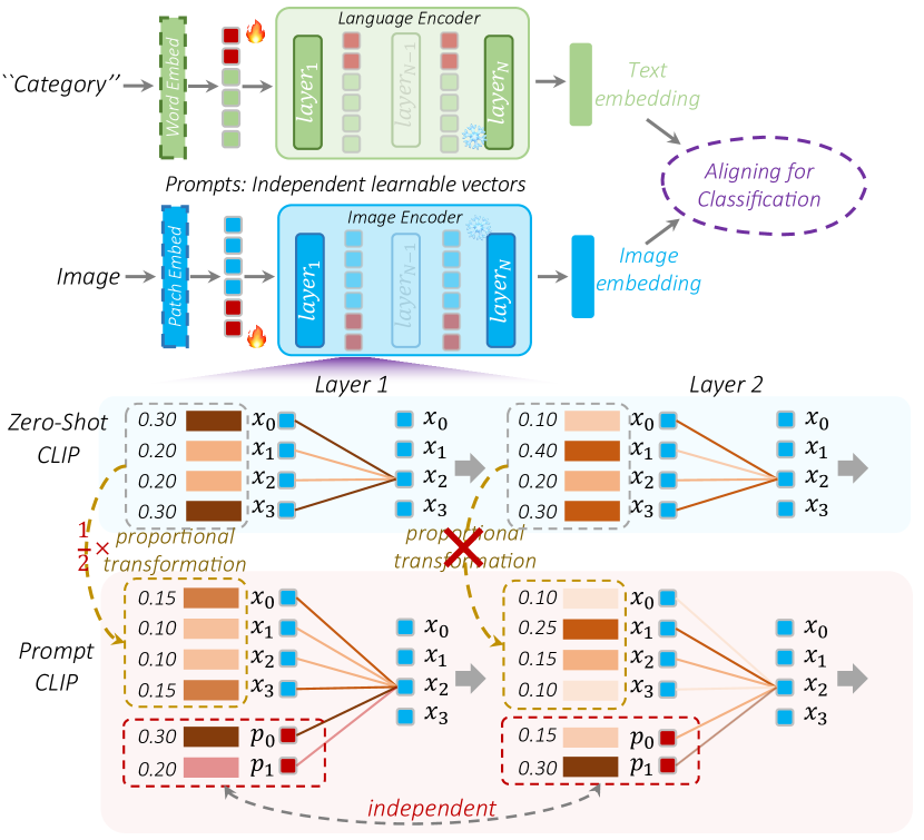
Figure 1: Overscheme of the multi-modal prompts in the pre-trained model. In each layer, the fixed prompts provide additional attention value for each token. In the first layer, the attention between tokens undergoes a proportional transformation ($\frac{1}{2}\times$). However, the relative values of attention between tokens are changed in the subsequent layers. Detailed explanation in Sec.3.2.1.

The pre-trained Vision-Language (VL) models [28, 16, 40, 37, 38] are pre-trained on a large corpus of image-text pairs available on the internet, such as CLIP400M and ALIGN1B, in a self-supervised manner. They possess a strong understanding of open-vocabulary concepts, making them suitable for various downstream vision and vision-language applications [12, 41, 30, 23, 45, 13, 25, 39, 21, 29, 10]. However, their zero-shot performance is unsatisfactory in many specific datasets, especially those with significant differences from natural language and images. It is crucial to tune these pre-trained models to specific datasets.

Prompt tuning [43, 44, 6, 15, 32, 22, 1, 18, 31, 19] has emerged as a more efficient alternative to fine-tuning large-scale models. This approach introduces a small number of new learnable embeddings at the input, known as prompt tokens, to adapt the pre-trained models for downstream tasks while keeping the pre-trained model weights fixed, as shown in Fig.1. Due to its efficiency in terms of parameters and convergence rate, prompt learning is found to be of great interest for adapting foundational models like CLIP for vision [17, 42, 34, 35] and vision-language tasks [44, 43, 46, 9]. However, despite the progress in the development of prompt tuning, their design is still driven empirically, and a good understanding of their essential attribute is lacking.

This paper attempts to explain the mechanism of the learned multi-modal prompts from the perspective of attention statistics and visualization. We begin with leveraging the formula to separate the part of the prompts workspace in the encoder. We observe that prompts primarily work for the self-attention block of each layer in two ways, as shown in Fig.1. $(i)$ prompts adapt the attention weights between the $[cls]$ token and the input tokens by assigning different attention weights to input tokens according to the similarity between the prompts and the corresponding tokens (detail in Sec.3.2.1). $(ii)$ the learned prompts serve as the additional fixed tokens to provide fixed features to the $[cls]$ and input tokens. We then probe the working ways of the prompts through the alignment contribution statistic and the separate analysis for image and language branches.

In the alignment contribution statistic, we count the relevance between inputs and $[cls]$ token during alignment. In the statistics results of the text branch, we observe that the contribution of category tokens does not increase but decreases. On the contrary, the contribution of $t_{SOS}$ and prompt tokens significantly increased, especially the $t_{SOS}$ token. For the image branch, we reveal that the learned multi-modal prompts do not significantly adjust the relative relevance to $[cls]$ between inputs. Surprisingly, the contribution of multi-modal prompts to the alignment process is significant.

In the language branch, we find CLIP’s textual branch primarily focuses on the $\bm{t}_{SOS}$ token, which serves as the bias. We attribute this as bias because the $\bm{t}_{SOS}$ token can not acquire the information from the input language features due to the casual self-attention mask mechanism. The learned text prompts enhance the model’s recognition performance on the relevant dataset by learning dataset biases and increasing the contribution of biases to the alignment task.

In the vision branch, by probing the average attention distance, attention entropy and visualizing the attention of the $[cls]$ token, we observe that the prompts do not significantly alter the feature extraction process of the pre-trained model, which further supports the second working mechanism of prompts. Meanwhile, by examining the similarity heatmap of learned vision prompts, we find that the vision prompts resemble background features to the attention of the $[cls]$ token, i.e., the features that the $[cls]$ token did not pay attention to. Combining the experimental phenomena in contribution statistics, we find that the prompts can act as a bridge to enable the $[cls]$ token to focus on background features that it previously overlooked. Because the learned prompts are independent and not updated by the input features, we believe that visual prompts, similar to text prompts, also act as dataset bias, which is important to the alignment.

Based on our findings, we propose a novel bias tuning that directly incorporates the learnable bias to each transformer block to validate the importance of the dataset bias. Comparative experiments demonstrate that bias tuning outperforms prompt tuning with the same number of parameters, particularly on datasets with limited category information, i.e., EuroSAT [14]. However, the drawbacks of directly learning bias are also evident, namely the limited design options for bias and the finite number of learnable parameters in each layer. In contrast, there is a wide variety of prompt options that can be added in each layer. To search for the optimal hyperparameter of the prompt for each dataset, we ablate on the number and layer of prompts. Bias tuning still falls slightly short compared to the optimal prompt configuration. However, for datasets with limited category information, the advantages of bias tuning remain highly evident.

Main Findings and Contributions: (1) We probe to understand the working mechanism of the multi-modal prompts for the pre-trained vision-language model, conducting a series of extensive experiments from various perspectives, including alignment relevance, attention, attention distance, attention entropy, and visualization. Our findings show that the prompts mainly learn as the dataset bias. (2) Based on the findings, we propose a novel bias tuning that directly incorporates the learnable bias to each transformer block. Our bias tuning outperforms prompt tuning with the same number of parameters, particularly on datasets with limited category information, i.e., EuroSAT [14].

2 Preliminaries

2.1 Vision-Language Pre-trained Model (VLM)

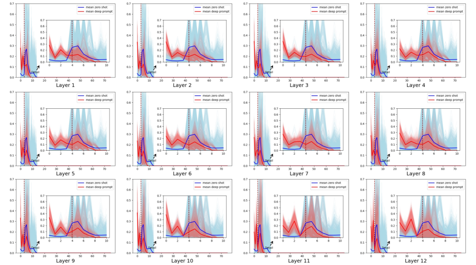
Figure 2: Statistics results on the contribution of each token of the language branch to the alignment task for the OxfordPet dataset. The corresponding two realizations are averaged over the statistics for the entire dataset, where the blue and red regions represent the statistics for zero-shot and prompt tuning, respectively. On the left side of the red vertical line, we show the contribution of the $\bm{t}_{SOS}$ token followed by four learned text prompts $\bm{P}_{t}$. On the right side, we show the $\bm{c}_{k}$ tokens and padding tokens. The horizontal coordinate is the index of the token and the vertical coordinate is the relative value of the contribution. For the zero-shot clip, we use the temple: ‘‘a photo of [Category].’’. For the tokens after the $\bm{t}_{EOS}$, we set their contribution as 0 for intuitive comparison. Meanwhile, we zoom in on comparing the index at which the prompt is placed in the middle of each figure. The statistics results of other datasets are detailedly shown in the Appendix.

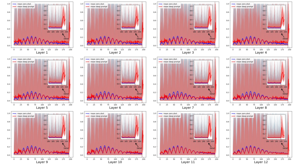
Figure 3: Statistics results on the contribution of each patch of the image branch to the alignment task for the OxfordPet dataset. The corresponding two realizations are averaged over the statistics for the entire dataset, where the blue and red regions represent the statistics for zero-shot and prompt tuning, respectively. On the left side of the red vertical line, we show the contribution of the input patch tokens $\bm{\tilde{X}_{p}}$. On the right side, we show the learned vision prompts $\bm{P}_{v}$. The horizontal coordinate is the index of the token and the vertical coordinate is the relative value of the contribution. For the zero-shot clip, the values of the 196th-199th index are empty due to the absence of the vision prompts. Meanwhile, we zoom in on comparing the index at which the prompt is placed in the middle of each figure. The statistics results of other datasets are detailedly shown in the Appendix.

We represent the vision and text encoders as ${f}$ and ${g}$, respectively. The pre-trained parameters are denoted as ${\theta}_{\mathtt{VLM}}=\{\theta_{f},\theta_{g}\}$. The input image $\bm{X}\in\mathbb{R}^{C\times H\times W}$ is divided into $M$ patches $\left\{{patch}^{1};\cdots;{patch}^{M}\right\}$ followed by a projection $\mathbf{E}\in\mathbb{R}^{\left(\frac{HW}{M}\cdot C\right)\times D_{v}}$ to produce patch tokens $\{\bm{x}_{1},\bm{x}_{2},\cdots,\bm{x}_{M}\}$. Further, a learnable class token $\bm{x}_{cls}$ is attached to the input patches as $\bm{\tilde{X}}=\{\bm{x}_{cls},\bm{x}_{1},\bm{x}_{2},\cdots,\bm{x}_{M}\}$. After adding the position embeddings $\bm{E}_{pos}\in\mathbb{R}^{(M+1)\times D_{v}}$, the input patches are encoded by the encoder ${f}$ via $L_{v}$ transformer blocks in the bi-directional self-attention mask to produce the visual feature representation $\bm{\tilde{f}}=f(\bm{\tilde{X}},\theta_{f})$, where $\bm{\tilde{f}}\in\mathbb{R}^{d}$. The detailed formulation is as follows:

$$\mathbf{x}_{0} =\left[\bm{x}_{cls};\bm{x}_{1};\bm{x}_{2};\cdots,\bm{x}_{M}\right]+\bm{E}_{pos},$$ (1)

$$\mathbf{x}_{\ell}^{\prime} =\mathtt{MSA}\left(\mathtt{LN}\left(\mathbf{x}_{\ell-1}\right)\right)+\mathbf{x}_{\ell-1},\ell=1\ldots L_{v},$$ (2)

$$\mathbf{x}_{\ell} =\mathtt{MLP}\left(\mathtt{LN}\left(\mathbf{x}_{\ell}^{\prime}\right)\right)+\mathbf{x}_{\ell}^{\prime},\ell=1\ldots L_{v},$$ (3)

$$\bm{\tilde{f}} =\mathtt{LN}\left(\mathbf{x}_{L}^{0}\right)@\ \mathbf{E_{v}},\mathbf{E_{v}}\in\mathbb{R}^{{D_{v}}\times{d}}.$$ (4)

For the language branch, the corresponding category label ${y}$ is wrapped within a text template such as ‘a photo of a {category}’ which can be formulated as $\bm{\tilde{Y}}=\{\bm{t}_{SOS},\bm{t}_{1},\bm{t}_{2},\cdots,\bm{t}_{n},\bm{c}_{k},\bm{t}_{EOS}\}$. Here $\{\bm{t}_{l}|_{l=1}^{n}\}$ and $\bm{c}_{k}$ denote the word embeddings corresponding to the text template and the class label, respectively. $\bm{t}_{SOS}$ and $\bm{t}_{EOS}$ are the learnable start and end token embeddings, respectively. Then, $\bm{\tilde{Y}}$ are encoded by the text encoder ${g}$ via $L_{t}$ transformer blocks in the casual self-attention mask to the textual feature $\bm{\tilde{g}}=g(\bm{\tilde{Y}},\theta_{g})$, where $\bm{\tilde{g}}\in\mathbb{R}^{d}$. The detailed formulation is as follows:

$$\mathbf{y}_{0} =\left[\bm{t}_{SOS},\bm{t}_{1},\bm{t}_{2},\cdots,\bm{t}_{n},\bm{c}_{k},\bm{t}_{EOS}\right]+\bm{E}_{pos},$$ (5)

$$\mathbf{y}_{\ell}^{\prime} =\mathtt{MSA}\left(\mathtt{LN}\left(\mathbf{y}_{\ell-1}\right)\right)+\mathbf{y}_{\ell-1},\ell=1\ldots L_{t},$$ (6)

$$\mathbf{y}_{\ell} =\mathtt{MLP}\left(\mathtt{LN}\left(\mathbf{y}_{\ell}^{\prime}\right)\right)+\mathbf{y}_{\ell}^{\prime},\ell=1\ldots L_{t},$$ (7)

$$\bm{\tilde{g}} =\mathbf{y}_{L}^{-1}@\ \mathbf{E_{t}},\mathbf{E_{t}}\in\mathbb{R}^{{D_{t}}\times{d}}.$$ (8)

During the zero-shot inference, textual features of text template with class labels $\{c_{1},c_{2},\cdots,c_{m}\}$ are matched with image feature $\bm{\tilde{f}}$, the category is predicted as follows:

$$\bm{pred}=\bm{argmax}(\frac{\mathtt{exp}(\mathtt{sim}(\bm{\tilde{g}},\bm{\tilde{f}})\tau)}{\sum_{i=1}^{{num}_{c}}\mathtt{exp}(\mathtt{sim}(\bm{\tilde{g^{i}}}\cdot\bm{\tilde{f}})\tau)}),$$ (9)

where $\mathtt{sim}(a,b)$ denotes the cosine similarity between $a$ and $b$, and $\tau$ is the temperature.

2.2 Multi-Prompt Learning for VLM

The multi-modal prompts learn hierarchical prompt tokens on both the text and image encoders separately. The independent multi-modal prompts append learnable $T$ language and $V$ visual prompts given as $\bm{P_{t}}=\{\bm{p_{t}}^{1},\bm{p_{t}}^{2},\cdots,\bm{p_{t}}^{T}\}$ and $\bm{P_{v}}=\{\bm{p_{v}}^{1},\bm{p_{v}}^{2},\cdots,\bm{p_{v}}^{V}\}$ with the textual categories and visual input tokens, respectively. The image encoder processes all tokens $\bm{\tilde{X}_{p}}=\{\bm{e}_{cls},\bm{e}_{1},\bm{e}_{2},\cdots,\bm{e}_{M},\bm{p_{v}}^{1},\bm{p_{v}}^{2},\cdots,\bm{p_{v}}^{V}\}\}$ to generate prompted visual feature $\bm{\tilde{f}_{p}}$. In the self-attention blocks, the prompts provide additional fixed features for the updating of the $[cls]$ token and patch tokens.

Similarly, the text branch formulation is omitted, and the textual feature $\bm{\tilde{g}_{p}}$ is acquired, where $\bm{\tilde{Y}_{p}}=\{\bm{t}_{SOS},\bm{p^{1}_{t}},\bm{p}^{2}_{t},\bm{p}^{3}_{t},\cdots,\bm{p}^{T}_{t},c_{k},\bm{t}_{EOS}\}$. In this paper, we explore the independent deep multi-modal prompts. The vision and language prompts are jointly represented as $\bm{P}=\{\bm{P_{v}},\bm{P_{t}}\}$. For image classification on the downstream dataset $\mathcal{D}$, prompts $\bm{P}$ are inserted into the pre-trained and frozen $\theta_{f}$ and $\theta_{g}$ and are optimized with the cross-entropy loss, $\mathcal{L_{\text{CE}}}$, as follows:

$$\mathcal{L_{\text{CE}}}=\text{arg} \min_{\bm{P}}\mathbb{E}_{(\bm{X},{y})\sim\mathcal{D}}\,\mathcal{L}(\text{sim}(\bm{\tilde{f}_{p}},\bm{\tilde{g}_{p}}),y).$$ (10)

In the inference phase, the model predicts with the learned multi-prompts as follows:

$$\bm{pred}=\bm{argmax}(\frac{\mathtt{exp}(\mathtt{sim}(\bm{\tilde{g}_{p}},\bm{\tilde{f}_{p}})\tau)}{\sum_{i=1}^{C}\mathtt{exp}(\mathtt{sim}(\bm{\tilde{g_{p}^{i}}}\cdot\bm{\tilde{f}_{p}})\tau)}).$$ (11)

This paper aims to investigate the mechanism of the multi-modal prompts through the perspective of attention through statistical and visualization experiments.

3 Exploring Experimrnts

3.1 Experiment Setting

Implementation Details: We use the ViT-B/16 CLIP model in all experiments. Following the existing methods [43, 18], we uniformly train a few epochs, i.e., 10, using the $SGD$ optimizer, for preventing the model from overfitting to the few-shot data. We use the $cosine$ learning scheduler, and the learning rate is uniformly set as 0.0025. Meanwhile, we set the first epoch as the warmup epoch, and the warmup type and warmup constant learning rate are set as constant and 1e-5, respectively. In this paper, we conduct the exploring experiments in the 16-shot setting. The batch size is uniformly set as 32, and we did not search for specific suitable hyperparameters for individual datasets to improve the performance.

Datasets: We use 11 image recognition datasets. The datasets cover multiple recognition tasks including ImageNet [8] and Caltech101 [11] that consist of generic object categories. OxfordPets [27], StanfordCars [20], Flowers102 [26], Food101 [2], and FGVCAircraft [24] have fine-grained categories. SUN397 [36] and UCF101 [33] are specific for scene and action recognition, respectively. DTD [7] has diverse texture categories and EuroSAT [14] consists of satellite images.

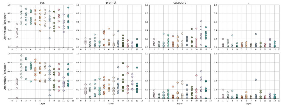
Figure 4: Statistics results on the $[cls]$ token attention for the ImageNet dataset. The first row is the attention distribution of CLIP, where the prompt denotes ‘a photo of a’. The second row is the feature distribution after adding the vision prompts, where the prompt represents the learnable token. Each graph contains the attention distribution of 12 transformer blocks, and each data layer includes 8 attention heads. sos, prompt, category and ‘.’ denote the $[cls]$ token’s attention on the corresponding token.

3.2 How do the prompts improve the performance?

3.2.1 Attention Formulation

Adding the multi-modal prompts, which learn from the few-shot training, often results in substantial recognition performance gains. Although the multi-modal prompts serve as tokens similar to the input tokens, it is also not rational to intuitively conclude how they work, since they are all at the high latitude abstraction space level, and we cannot determine what kind of image or text is learned. For the vision/text encoder, which consists of self-attention and MLP block, we analyze the impact of the added prompts in turn. For the MLP that attributes with independent operations for inputs, the added prompts through concatenate operations do not affect the upgrade of the input tokens. For self-attention layers, the prompts affect the attention weights of the $[cls]$ and input tokens in the attention calculation. We take the visual branch as an example to derive, after adding the prompt token $\bm{\tilde{X}}=\{\bm{x}_{cls},\bm{x}_{1},\bm{x}_{2},\cdots,\bm{x}_{M}\}$ $\rightarrow$ $\bm{\tilde{X}_{p}}=\{\bm{x}_{cls},\bm{x}_{1},\bm{x}_{2},\cdots,\bm{x}_{M},\bm{p_{v}}^{1},\bm{p_{v}}^{2},\cdots,\bm{p_{v}}^{V}\}\}$ (as shown in the Sec.2, in the image branch $\bm{x_{0}}$ denotes $\bm{x_{cls}}$). The updated process changes as follows:

$$\bm{x_{i}^{\ell+1}} =\bm{x_{i}^{\ell}+\sum_{j=0}^{M}\underline{\underline{a_{ij}}}\cdot x_{j}},$$ (12)

$$\ \ \quad\quad\downarrow$$

$$\bm{x_{i}^{\ell+1}} =\bm{x_{i}^{\ell}+\sum_{j=0}^{M}\underline{\underline{a_{ij}^{\prime}}}\cdot x_{j}}\bm{+}\underline{\underline{\bm{\sum_{k=0}^{V}a_{ik}^{\prime}\cdot p_{v}^{k}}}},$$

Where $\bm{a_{ij}},\bm{a^{\prime}_{ij}}\propto\bm{e^{x_{i}Ax_{j}}}$, $\bm{a^{\prime}_{ik}}\propto\bm{e^{x_{i}Ap^{k}_{v}}}$ and $A=\frac{\bm{QK}^{T}}{\bm{\sqrt{d}}}$, $\bm{Q}$, $\bm{K}\in\mathbb{R}^{{D_{v}}\times{D_{v}}}$ are projection matrix. The detailed formulation is shown in the Appendix. For the deep independent multi-modal prompts, the prompts are independently learned at each layer; once learned, they become a fixed piece of information for all data in the dataset, similar to the concept of bias. However, we observe that the information provided by the prompts is closely related to the patch tokens. That is, the more similar $x_{i}$ is to $p_{c}$, the larger the attention value obtained. Therefore, the information obtained by tokens from prompts in each layer differs. This results in changes to the values of the tokens in the subsequent layers, and the magnitude of these changes varies. As a result, the relative attention in the subsequent layers between tokens also changes. Thus, we make the following hypothesis about the working mechanism.

• Prompts improve the recognition performance mainly by adapting the attention values between the $[cls]$ token and the input tokens according to assigning different attention weights to input tokens. This means that the attention distribution of the $[cls]$ token towards the input tokens may be affected for better direction, leading to a better focus of the $[cls]$ token on foreground objects, which is crucial for classifying individuals.

• Prompts mainly improve recognition performance by learning a bias term during the update of token embeddings, allowing the model to adapt to the target domain. This means fixed prompts may provide fixed dataset bias information at each layer after learning the corresponding dataset for better alignment between the image and language embeddings.

• Both of the above are indispensable.

To investigate and validate the aforementioned hypothesis, we conducted a series of subsequent statistical and visualization experiments.

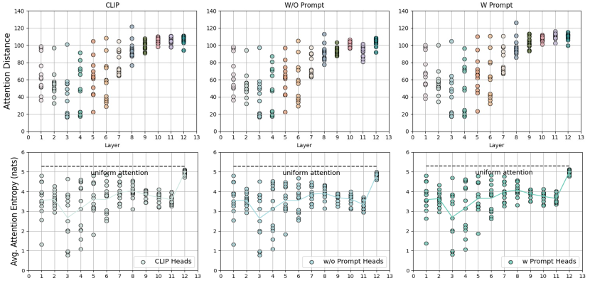
Figure 5: The averaged attention distance and entropy in different attention heads (dots). For the CLIP, we statistic the averaged attention distance and entropy of the original CLIP model. For the W/O Prompt, we statistic the averaged attention distance and entropy of the CLIP model after adding the prompts, but we remove the attention distance of the prompts. For the W Prompt, the attention distance and entropy of the prompts are retained.

3.2.2 Aligning Contribution Statistics

We start by examining the contributions of each patch and token in the alignment process of the corresponding image-text pairs. For the contribution of each branch, we statistic the relevance of all tokens, including prompt tokens, to the $[cls]$ token before and after adding the learned prompts. Following [4, 5], we construct a relevancy map per interaction, i.e. $\mathtt{R}^{tt}$ and $\mathtt{R}^{vv}$ for language and vision modality, respectively. We calculate the relevancy maps by the forward pass on the attention layers, where each layer contributes to the aggregated relevance matrices. Before each modality self-attention operation, each patch/token is self-contained. Thus, the self-attention interactions are initialized with the identity matrix as follows:

$$\mathtt{R}_{0}^{vv}=\mathbb{I}^{v\times v},\quad\mathtt{R}_{0}^{tt}=\mathbb{I}^{t\times t}.$$ (13)

Immediately following each modality’s self-attention blocks, we utilize attention maps $\mathtt{A}=\operatorname{softmax}\left(\frac{\mathtt{Q}\cdot\mathtt{K}^{\top}}{\sqrt{d_{h}}}\right)$ to update the relevance matrices. $\mathtt{A}$ intuitively defines connections between each pair of tokens (in language modality) / patches (in vision modality). The relevancies are accumulated by adding each layer’s contribution to the aggregated relevancies due to the residual connection in the transformer blocks. All $h$ across head attention maps are averaged by the gradients that follow [4, 5]. Meanwhile, the simple average across heads would result in distorted relevancy maps because attention heads differ in importance and relevance. Thus, we follow [5] and define the final attention map $\overline{\mathtt{A}}$ as follows:

$$\overline{\mathtt{A}}=\mathbb{E}_{h}\left((\nabla\mathtt{A}\odot\mathtt{A})^{+}\right),$$ (14)

where $\mathbb{E}_{h}$ represents the mean across the head dimension, $\odot$ denotes the Hadamard product, $\nabla\mathtt{A}:=\frac{\partial y_{t}}{\partial\mathtt{A}}$ for $y_{t}$ which is the model’s output for the alignment target we wish to visualize. After obtaining the attention maps $\overline{\mathtt{A}}$ corresponding to each self-attention module of each modality, the final relevancy scores $\mathtt{R}^{vv},\mathtt{R}^{tt}$ are as follows:

$$\mathtt{R}_{\ell}^{vv} =\mathtt{R}_{\ell-1}^{vv}+\overline{\mathtt{A}}_{\ell-1}\cdot\mathtt{R}_{\ell-1}^{vv},$$ (15)

$$\mathtt{R}_{\ell}^{tt} =\mathtt{R}_{\ell-1}^{tt}+\overline{\mathtt{A}}_{\ell-1}\cdot\mathtt{R}_{\ell-1}^{tt}.$$ (16)

Finally, to retrieve per-token/patch relevancies for the alignment, we consider the row corresponding to the $[cls]$ token in the vision modality and the $\bm{t}_{EOS}$ in the language modality, which describes the connection between the $[cls]$ or $\bm{t}_{EOS}$ token and the other image patches/text tokens, i.e. $\mathtt{R}_{\ell}^{vv}\left[\mathtt{:},\ \mathtt{0},\ \mathtt{1:}\right]$, $\mathtt{R}_{\ell}^{tt}\left[\mathtt{:},\ \mathtt{-}1,\ \mathtt{:-1}\right]$.

To visually illustrate the dependency of alignment tasks on image patches and text tokens after incorporating prompts, we conduct a statistical analysis on eleven fine-grained recognition datasets. Before visualization, we preprocess the contribution according to normalization for intuitive comparison. The distribution of relevance for the OxfordPet dataset is presented in Fig.2 and Fig.3 (Ten more other datasets are shown in the Appendix).

• In the statistics results of the text branch, we observe that the contribution of category tokens does not increase but decreases. On the contrary, the contribution of $t_{SOS}$ and prompt tokens significantly increased, especially the $t_{SOS}$ token.

• For the image branch, we reveal that the learned multi-modal prompts do not significantly adjust the relative relevance to $[cls]$ between inputs. Although there may be differences in the absolute values between tokens or patches in the statistical table, this is mainly due to normalization operations, and the actual relative changes are minimal. On the contrary, the contribution of multi-modal prompts to the alignment process is unusually prominent.

Therefore, from the alignment contribution statistics, we observe that the mechanism of prompts better aligns with the second way in Sec.3.2.1. Below, we further delve into the investigation by studying what prompts learn and how they influence the alignment process in the language and image branches, respectively.

3.3 What do the multi-modal prompts learn?

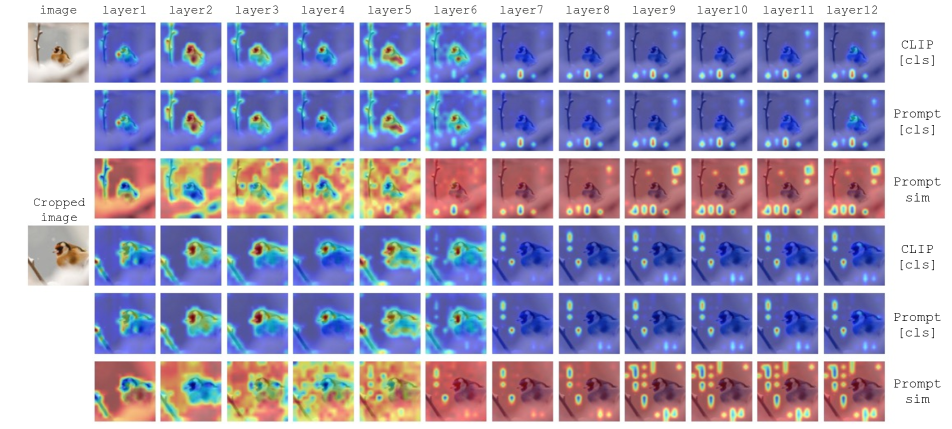
Figure 6: Visualization results on the $[cls]$ token attention and vision prompts similarity on input patches for the ImageNet dataset. Where the first and second row is the $[cls]$ token attention on the input patches of original CLIP and prompt CLIP, the layer corresponds to the encoder transformer block. The last row is the vision prompts’ similarity with the input tokens.

The multi-modal prompts are situated within a high-dimensional space, assuming a role that is equivalent to that of input features (image patches/language tokens) of the same level. Hence, while it may not be possible to visualize the prompt as concrete images and text directly, we can showcase the prompt by visualizing the distribution of its similarity to the input features at the same level. In this section, we explore the text and vision prompts through attention and similarity.

3.3.1 Learned Textual prompts on Language Branch

For the text encoder, CLIP leverages the attention way of GPT [3], where the former token can not focus on the latter tokens. Thus, the last token called $\bm{t}_{EOS}$ takes on the role of $[cls]$ token. In the language branch, we explore the textual prompts by the statistical attention distribution between the $\bm{t}_{EOS}$ takes and all other tokens, i.e., $\bm{t}_{SOS}$, $\bm{P}_{t}$ and $\bm{c}_{k}$, as shown in 4.

From the zero-shot CLIP attention statistics results in the first row of Fig.4, we observe that the $\bm{t}_{EOS}$ predominantly focuses most of its attention on the $\bm{t}_{SOS}$ token in each layer. However, the $\bm{t}_{SOS}$ token cannot attend to the subsequent category information, so its role is merely that of a bias. Meanwhile, We find that the text prompts play a role similar to the $\bm{t}_{SOS}$ token, as they also precede the category information and represent fixed information learned from the entire dataset without being updated based on the category information. The only difference is that the $\bm{t}_{SOS}$ token learns biases based on the entire language domain, as CLIP [28] is pre-trained on a massive amount of image-text pairs, while the text prompts only learn biases specific to the corresponding dataset.

We observe that after incorporating the learned text prompts, the attention of $\bm{t}_{EOS}$ towards $\bm{t}_{SOS}$ significantly decreases, while its attention towards the prompts noticeably increases. Meanwhile, the attention toward category tokens stays the same. Combining the findings from Sec.3.2.2 and the results in Fig.2, we conclude that learned text prompts transfer some of the attention of $\bm{t}_{EOS}$ on $\bm{t}_{SOS}$ towards themselves, prompting the pre-trained model to shift some of the attention from the entire text domain biases to biases specific to the relevant dataset. As a result, it enhances the model’s discriminative performance on the corresponding dataset.

3.3.2 Vision prompts on Image Branch

In the image branch, we explore the vision prompts in the following ways: (i) Probing the average attention distance. (ii) Probing the attention entropy of the attention weight and $[cls]$ attention. (iii) Visualizing $[cls]$ token’s attention on the image patches and the similarity distribution between the vision prompts and image patches.

Attention Distance: To probe the impact of incorporating vision prompts on the feature extraction mechanism of the encoder, we analyze the average attention distance of the model before and after adding prompts, as shown in the first row of Fig.5. From the statistical results comparison of the CLIP, W/O Prompt and W Prompt, we observe that there is no significant impact on the model’s attention distance before and after incorporating prompts for the input patches. This indicates that prompts do not significantly alter the feature extraction process of the pre-trained model. This further supports the second working mechanism of prompts in Sec.3.2.1.

Attention Entropy: We analyze the model’s attention before and after adding prompts and show the results in the second row of Fig.5 for probing the impact of incorporating vision prompts on the vision encoder’s feature extraction mechanism. The entropy value of attention reflects the focus of attention. A higher entropy value indicates a more uniform attention distribution and a global focus of attention. A lower entropy value indicates a more extreme attention distribution and a local focus of attention. From the results, we obtained the same conclusion as the attention distance statistic results: the prompts do not significantly impact the attention scope.

visualization: For the $[cls]$ token attention, we visualize the attention as the heatmap, as shown in Fig.6. For the vision prompt similarity distribution, we calculate the Euclidean distance between the vision prompts and image patches. Due to the negative correlation between distance and similarity, after interpolation and normalization, we apply a linear transformation to the distance map by taking its complement, i.e., $\mathtt{x}=\mathtt{1}-\mathtt{x}$. To increase input diversity and showcase more detailed visual comparisons, we introduce rotation operations for the vision input, as shown in Fig.6. From the visualization results, we observe that the vision prompts do not influence $[cls]$ token’s attention on the input patches, which further supports the second working mechanism of prompts in Sec.3.2.1.

Meanwhile, Fig.6 visually demonstrates that the learned vision prompts resemble background features in relation to the attention of the $[cls]$ token, i.e., the features that the $[cls]$ token did not pay attention to. Since Fig.3 shows that the attention of the $[cls]$ token towards the prompt is significant, we conclude that the prompt can act as a bridge to enable the $[cls]$ token to focus on background features that it previously overlooked. Furthermore, considering the fact that the learned prompts are independent and not updated by the input features, we believe that visual prompts, similar to text prompts, also act as dataset bias.

3.4 Validation for the importance of the bias

To validate the conclusion, we directly add the learnable bias to the pre-trained model and compare it with the prompt tuning. In the bias tuning setting, we add an independent learnable embedding and repeat it to add to all tokens after each transformer layer of the image and language branch. After learning in the same few-shot setting, we compare the bias tuning, prompt tuning, and zero-shot CLIP in Table.1. The results show that bias tuning outperforms prompt tuning, especially on datasets with single-category information and scenes, such as EuroSAT [14]. However, prompt tuning has an advantage over bias tuning in that their performance can improve with an increase in the number of prompts. Table.1 shows the slight performance gap (0.5) between bias tuning and the optimal prompt tuning settings (acquired from the sensitivity analysis results in the Appendix) still exists.

Table 1: Validating the importance of bias. We compare bias with prompt tuning in the same parameter and the optimal settings.

Dataset	CLIP	PROMPT	BIAS	OPTIMAL
ImageNet [8]	66.7	72.5	71.9	73.1
Caltech101 [11]	93.3	95.2	96.0	95.2
DTD [7]	44.1	68.8	69.6	70.5
EuroSAT [14]	48.4	71.7	86.5	82.6
FGVCAircraft [24]	24.9	37.7	41.0	40.9
Food101 [2]	85.9	87.3	86.0	87.1
OxfordFlowers [26]	70.7	94.7	94.7	96.5
OxfordPets [27]	89.1	93.6	92.7	93.1
StanfordCars [20]	65.6	76.6	77.7	80.5
SUN397 [36]	62.6	75.3	74.7	76.2
UCF101 [33]	67.5	82.1	83.5	84.2
AVERAGE	65.3	77.8	79.5	80.0

3.5 Sensitivity Analysis for Multi-Modal Prompts

We analyze the robustness and sensitivity of the multi-modal prompts. The detailed results are shown in the Appendix.

Prompt Layer: We observe that the performance of the multi-modal prompts increases as the number of layers increases, but the upward trend also gradually slows down. Meanwhile, we observe that different datasets have different optimal numbers of layers. For datasets with many categories, such as ImageNet [8], the performance continues to increase with more layers. However, for datasets with fewer categories and high similarity between categories, such as EuroSAT [14], the performance saturates after adding a smaller number of multi-modal prompt layers.

Prompt Number:Increasing the number of prompts can improve performance in the pre-trained model. However, when the number becomes excessive, the stability of the learning process decreases. We observe that when the number of multi-modal prompts exceeds 20, the learning process of the prompts becomes highly unstable and prone to failure, especially for datasets with limited category information such as EuroSAT [14].

4 Conclusion

This paper probes to understand the working mechanism of the multi-modal prompts for the pre-trained vision-language model, conducting a series of extensive experiments from various perspectives, including alignment relevance, attention, attention distance, attention entropy, and visualization. Our findings show that the prompts mainly learn as the dataset bias. Based on the findings, we propose a novel bias tuning that directly incorporates the learnable bias to each transformer block that outperforms prompt tuning with the same number of parameters, particularly on datasets with limited category information.

In the appendix, we provide detailed theoretical derivations and experimental support for the review manuscript from the following perspectives:

• In Sec.A, We provide a detailed introduction to the works related to this paper, including visual-language pre-training models and prompt learning approaches.

• In Sec.B, we detailedly compare the attention computation process in the transformer encoder before and after incorporating the prompt via the formulation.

• We provide ablation experiment results for the eleven fine-grained datasets in Sec.C.

• In Sec.D, we provide more detailed attention-entropy statistic results.

• We provide contribution statistic results for more fine-grained datasets for the comparison between CLIP, Shallow Prompt, and Deep Prompt in Sec.E.

Appendix A Related Works

A.1 Vision Language models

Foundational vision-language (VL) models [28, 16, 40, 37, 38] leverage both visual and textual modalities to encode rich multi-modal representations. These models are pre-trained on a large corpus of image-text pairs available on the internet in a self-supervised manner. For instance, CLIP [28] and ALIGN [16] utilize around 400M and 1B image-text pairs, respectively, to train their multi-modal networks. During pre-training, contrastive loss is commonly used as a self-supervision loss. This loss pulls together the features of paired images and texts while pushing away the unpaired image-text features. VL models possess a strong understanding of open-vocabulary concepts, making them suitable for various downstream vision and vision-language applications [12, 41, 30, 23, 45, 13, 25, 39, 21, 29, 10]. However, transferring these foundational models for downstream tasks without compromising on their original generalization ability still remains a major challenge. Our work aims to address this problem by proposing a novel regularization framework to adapt VL models via prompt learning.

A.2 Prompt learning

Prompt learning is an alternative fine-tuning method for transferring a model towards downstream tasks without re-learning the trained model parameters. This approach adapts a pre-trained model by adding a small number of new learnable embeddings at the input known as prompt tokens. Due to its efficiency in terms of parameters and convergence rate, prompt learning is found to be of great interest for adapting foundational models like CLIP for vision [17, 42, 34, 35] and vision-language tasks [44, 43, 46, 9]. CoOp [44] fine-tunes CLIP by optimizing a continuous set of prompt vectors in its language branch for few-shot image recognition. Bahng et al. [1] perform visual prompt tuning on CLIP by learning prompts on the vision branch. [6] and [22] propose to learn multiple sets of prompts for learning different contextual representations. CoCoOp [43] highlights the overfitting problem of CoOp and proposes to condition prompts based on visual features for improved performance on generalization tasks. MaPLe [18] proposes a multi-modal prompt learning approach by learning hierarchical prompts jointly at the vision and language branches of CLIP for better transfer. Our approach builds on a variant [31] where prompts are learned at both the vision and language encoder of CLIP.

Appendix B Detailed Formulation

Adding the multi-modal prompts, which learn from the few-shot training, often results in substantial recognition performance gains. Although the multi-modal prompts serve as tokens similar to the input tokens, it is also not rational to intuitively conclude how they work, since they are all at the high latitude abstraction space level, and we cannot determine what kind of image or text is learned. For the vision/text encoder, which consists of self-attention and MLP block, we analyze the impact of the added prompts in turn. For the MLP that attributes with independent operations for inputs, the added prompts through concatenate operations do not affect the upgrade of the input tokens. For self-attention layers, the prompts affect the attention weights of the $[cls]$ and input tokens in the attention calculation. We take the visual branch as an example to derive, after adding the prompt token ${X}$ $\rightarrow$ ${X_{p}}=[X,P]$ (in the image branch ${x_{0}}$ denotes ${x_{cls}}$). The detailed self-attention calculation process is shown as follows:

Before adding the prompts:

$$\Delta x_{i} =\operatorname{softmax}\left(\frac{x_{i}\cdot Q\cdot(X\cdot K)^{T}}{\sqrt{d}}\right)\cdot X\cdot V$$ (17)

$$\quad\quad\quad\quad\quad\downarrow$$ (18)

$$=\operatorname{softmax}\left(\frac{x_{i}\cdot Q\cdot K^{T}\cdot X^{T}}{\sqrt{d}}\right)\cdot X\cdot V$$ (19)

$$\quad\quad\quad\quad\quad\downarrow A\triangleq\frac{Q\cdot K^{T}}{\sqrt{d}}$$ (20)

$$=\operatorname{softmax}\left(x_{i}\cdot A\cdot X^{T}\right)\cdot X\cdot V$$ (21)

$$\quad\quad\quad\quad\quad\downarrow$$ (22)

$$=\frac{\sum_{c=0}^{n}\left(e^{x_{i}Ax_{c}^{T}}\cdot x_{c}V\right)}{\sum_{c=0}^{n}e^{x_{i}Ax_{c}^{T}}}$$ (23)

After Adding the prompts:

$$\Delta x_{i} =\operatorname{softmax}\left(\frac{x_{i}\cdot Q\cdot([X,P]\cdot K)^{T}}{\sqrt{d}}\right)\cdot[X,P]\cdot V$$ (24)

$$\quad\quad\quad\quad\quad\quad\quad\quad\downarrow$$ (25)

$$=\operatorname{softmax}\left(\frac{x_{i}\cdot Q\cdot K^{T}\cdot\left[X^{T},P^{T}\right]}{\sqrt{d}}\right)\cdot[X,P]\cdot V$$ (26)

$$\quad\quad\quad\quad\quad\quad\quad\quad\downarrow A\triangleq\frac{Q\cdot K^{T}}{\sqrt{d}}$$ (27)

$$=\operatorname{softmax}\left(x_{i}\cdot A\cdot\left[X^{T},P^{T}\right]\right)\cdot[X,P]\cdot V$$ (28)

$$\quad\quad\quad\quad\quad\quad\quad\quad\downarrow$$ (29)

$$=\frac{\sum_{c=0}^{n}\left(e^{x_{i}Ax_{c}^{T}}\cdot x_{c}V\right)+\sum_{c=0}^{num_{p}}\left(e^{x_{i}Ap_{c}^{T}}\cdot p_{c}V\right)}{\sum_{c=0}^{n}e^{x_{i}Ax_{c}^{T}}+\sum_{c=0}^{nump}e^{x_{i}Ap_{c}^{T}}}$$ (30)

$$\quad\quad\quad\quad\quad\quad\quad\quad\downarrow$$ (31)

$$=\frac{\sum_{c=0}^{n}\left(e^{x_{i}Ax_{c}^{T}}\cdot x_{c}V\right)}{\sum_{c=0}^{n}e^{x_{i}Ax_{c}^{T}}+\sum_{c=0}^{num_{p}}e^{x_{i}Ap_{c}^{T}}}+\frac{\sum_{c=0}^{num_{p}}\left(e^{x_{i}Ap_{c}^{T}}\cdot p_{c}V\right)}{\sum_{c=0}^{n}e^{x_{i}Ax_{c}^{T}}+\sum_{c=0}^{num_{p}}e^{x_{i}Ap_{c}^{T}}}$$ (32)

In order to intuitively display the changes in attention before and after adding the prompt, we can simplify the formula as shown below where we simplify and omit the frozen parameters.

$$x_{i}^{\ell+1} =x_{i}^{\ell}+\sum_{j=0}^{M}\underline{\underline{a_{ij}}}\cdot x_{j},$$ (33)

$$\ \ \quad\quad\downarrow$$

$$x_{i}^{\ell+1} =x_{i}^{\ell}+\sum_{j=0}^{M}\underline{\underline{a_{ij}^{\prime}}}\cdot x_{j}+\underline{\underline{\sum_{k=0}^{V}a_{ik}^{\prime}\cdot p_{v}^{k}}},$$

Where ${a_{ij}},{a^{\prime}_{ij}}\propto{e^{x_{i}Ax_{j}}}$, ${a^{\prime}_{ik}}\propto{e^{x_{i}Ap^{k}_{v}}}$ and $A=\frac{{QK}^{T}}{{\sqrt{d}}}$, ${Q}$, ${K}\in\mathbb{R}^{{D_{v}}\times{D_{v}}}$ are frozen projection matrix. For the deep independent multi-modal prompts, the prompts are independently learned at each layer; once learned, they become a fixed piece of information for all data in the dataset, similar to the concept of bias. However, we observe that the information provided by the prompts is closely related to the patch tokens. That is, the more similar $x_{i}$ is to $p_{c}$, the larger the attention value obtained. Therefore, the information obtained by tokens from prompts in each layer differs. This results in changes to the values of the tokens in the subsequent layers, and the magnitude of these changes varies. As a result, the relative attention in the subsequent layers between tokens also changes. Thus, we make the following hypothesis about the working mechanism.

• Prompts improve the recognition performance mainly by adapting the attention values between the $[cls]$ token and the input tokens according to assigning different attention weights to input tokens. This means that the attention distribution of the $[cls]$ token towards the input tokens may be affected for better direction, leading to a better focus of the $[cls]$ token on foreground objects, which is crucial for classifying individuals.

• Prompts mainly improve recognition performance by learning a bias term during the update of token embeddings, allowing the model to adapt to the target domain. This means fixed prompts may provide fixed dataset bias information at each layer after learning the corresponding dataset for better alignment between the image and language embeddings.

• Both of the above are indispensable.

To investigate and validate the aforementioned hypothesis, we conducted a series of subsequent statistical and visualization experiments.

Table 2: Ablating the number of the multi-modal prompt layers. In each layer, the number of added multi-modal prompts is set to 8 which contains 4 vision prompts and 4 text prompts. The results are the average over seeds 1, 2, 3. More detailed results for each dataset and each seed are shown in the Appendix.

Method	CLIP[28]	Multi-Modal Prompt Layer
		1	2	3	4	5	6	7	8	9	10	11	12
ImageNet [8]	66.70	71.70	71.73	71.80	71.93	72.17	72.20	72.43	72.57	72.50	72.77	72.83	72.90
Caltech101 [11]	93.30	94.93	95.17	95.17	95.43	95.20	95.10	95.53	95.17	95.37	95.37	94.97	95.93
DTD [7]	44.10	62.13	64.20	65.07	64.97	65.00	66.13	67.47	67.93	67.77	68.53	68.53	69.20
EuroSAT [14]	48.40	48.53	67.07	73.53	78.33	77.17	78.37	79.67	82.50	82.30	82.87	81.83	77.87
FGVCAircraft [24]	24.90	34.23	32.93	34.17	35.83	35.97	36.27	37.20	38.40	38.87	38.93	39.93	39.37
Food101 [2]	85.90	87.17	86.93	87.37	87.07	87.30	87.23	87.33	87.30	87.33	87.23	87.40	87.23
OxfordFlowers [26]	70.70	91.83	92.77	92.93	94.50	94.47	95.07	95.27	95.60	96.00	96.00	96.03	95.83
OxfordPets [27]	89.10	92.57	93.03	93.13	93.00	93.50	93.37	93.53	93.43	93.43	93.73	93.70	93.33
StanfordCars [20]	65.60	73.70	74.63	75.57	75.87	76.27	77.23	78.20	78.10	79.07	79.13	79.30	78.60
SUN397 [36]	62.60	73.80	74.00	74.30	74.43	74.77	75.47	75.17	75.93	76.00	76.00	75.87	75.93
UCF101 [33]	67.50	78.40	79.33	80.17	80.27	80.97	81.83	81.67	82.17	83.03	82.53	82.70	83.33
Average	65.35	73.54	75.62	76.66	77.42	77.53	78.02	78.50	79.01	79.24	79.37	79.37	79.05

Appendix C Sensitivity Analysis for Multi-Modal Prompts

In this section, we analyze the robustness and sensitivity of the multi-modal prompts by examining the number of multi-modal prompt layers and multi-modal prompts. For the ablation experiments, we show the average results over three seeds, i.e., seeds 1, 2, 3.

C.1 Ablating the number of the prompt layers

For ablating the multi-modal prompt layers, we conduct an experiment over 11 recognition datasets  [8, 11, 7, 14, 24, 2, 26, 27, 20, 36, 33] where the performance on each dataset is compared by adding different layers of multi-modal prompts and showing the results in Table.2. In each layer, the number of added multi-modal prompts is set to 8, which contains 4 vision prompts and 4 text prompts. From the results in the table, we observe that the performance of the multi-modal prompts increases as the number of layers increases, but the upward trend also gradually slows down. Meanwhile, we observe that different datasets have different optimal numbers of layers. For datasets with a large number of categories, such as ImageNet [8], the performance continues to increase with the addition of more layers. However, for datasets with fewer categories and high similarity between categories, such as EuroSAT [14], the performance saturates after adding a smaller number of multi-modal prompt layers. With the addition of the 10 and 11-layer multi-modal prompts, the average performance reached its highest, exceeding CLIP by more than 14 points.

C.2 Ablating the number of prompts

In table.3, we ablate the number of multi-modal prompts. We set the number of layers to 12 and the number of text and vision prompts is the same for each layer. We set the number of multi-modal prompts to 2, 4, 6, 8, 20, 40, 100, i.e., the number of text and vision prompts is set to 1, 2, 3, 4, 10, 20, 50, respectively. We find that increasing the number of prompts can lead to improved performance in the pre-trained model. However, when the number becomes excessive, the stability of the learning process decreases. We observe that when the number of multi-modal prompts exceeds 20, the learning process of the prompts becomes highly unstable and prone to failure, especially for datasets with limited category information such as EuroSAT [14].

Table 3: Ablating the number of the multi-modal prompts. In the experiment, we set the number of layers to 12. The results are the average over seeds 1, 2, 3. More detailed results for each dataset and each seed are shown in the Appendix.

Method	IN[8]	C101[11]	DTD[7]	FGV[24]	F101[2]	Flowers[26]	Pets[27]	Cars[20]	SUN397[36]	UCF[33]	Euro[14]
CLIP[28]	66.70	93.30	44.10	24.90	85.90	70.70	89.10	65.60	62.60	67.50	48.40
2 prompts	72.50	95.17	68.77	37.73	87.27	94.73	93.57	76.63	75.33	82.13	71.73
4 prompts	72.63	95.67	68.63	37.27	87.37	95.63	93.60	77.77	75.70	82.53	76.53
6 prompts	72.90	95.47	69.50	39.90	87.40	95.87	93.23	79.00	75.97	82.97	79.37
8 prompts	72.90	95.93	69.20	39.37	87.23	95.83	93.33	78.60	75.93	83.33	77.87
20 prompts	73.13	95.20	70.47	40.93	87.07	96.47	93.07	80.50	76.23	84.17	82.60
40 prompts	72.97	95.73	70.73	41.90	87.03	96.20	93.53	81.10	76.03	84.27	-
100 prompts	72.77	95.57	68.53	42.47	86.40	96.20	92.97	81.33	76.20	83.83	-

Appendix D Attention Entropy

Attention Entropy: We analyze the attention of the model before and after adding prompts, as shown in the Fig.7, for probing the impact of incorporating vision prompts on the vision encoder’s feature extraction mechanism. The entropy value of attention reflects the focus of attention. A higher entropy value indicates a more uniform attention distribution and a global focus of attention. A lower entropy value indicates a more extreme attention distribution and a local focus of attention. In addition to calculating the attention entropy of all tokens in each layer, we also computed the attention entropy of the $[cls]$ token with respect to other tokens. From the results, we obtained the same conclusion as the attention distance statistic results: the prompts do not significantly impact the attention scope.

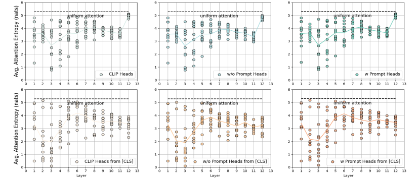
Figure 7: The attention entropy in different attention heads (dots). For the CLIP, we statistic the attention entropy and $[cls]$ token attention entropy of the original CLIP model. For the W/O Prompt, we statistic the attention entropy and $[cls]$ token attention entropy of the CLIP model after adding the prompts, but we remove the attention of the prompts. For the W Prompt, the attention of the prompts is retained.

Appendix E Alignment Contribution Statistic for CLIP, Shallow and Deep Prompt

In this section, we provide a detailed comparison of the alignment contribution between CLIP, Shallow Prompts, and Deep Prompts on other datasets. To ensure a fair comparison, we only compare on datasets where the clip template is fixed as “a photo of a + {} + {category}”. Since the templates for the DTD and EuroSAT datasets are “{} texture” and “a center satellite photo of + {category}” respectively, we do not make the comparison. Because the zero-shot performance of CLIP for the “a photo of a + {} + {category}” temple prompt on these two datasets is very bad. In the shallow prompt settings, we only add learned prompts in the first layer of the text and image encoder. In the deep prompt settings, we add learned prompts in all layers. We observe that in most datasets, the contribution of category tokens decreases after adding the learned prompt, while the contribution of the learned prompt tokens increases compared to that of template tokens. This phenomenon can be clearly observed in both shallow and deep prompts.

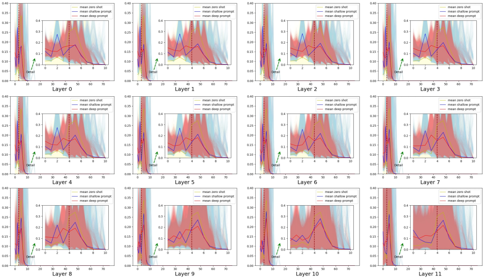
Figure 8: Statistics results on the contribution of each patch of the language branch to the alignment task for the ImageNet [8] dataset.

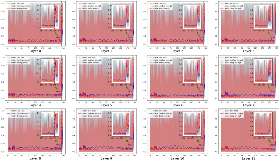
Figure 9: Statistics results on the contribution of each patch of the image branch to the alignment task for the ImageNet [8] dataset.

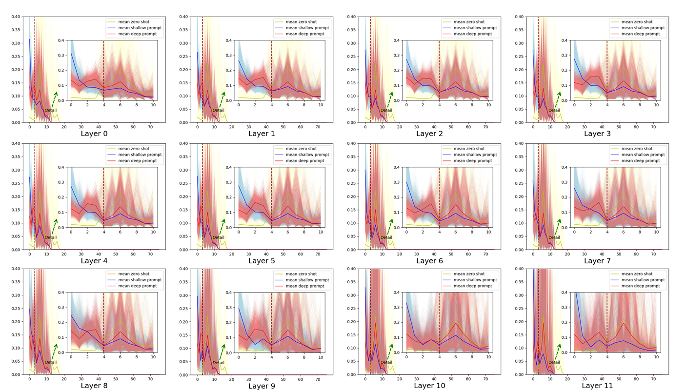
Figure 10: Statistics results on the contribution of each patch of the language branch to the alignment task for the FgvcAircrafat [24] dataset.

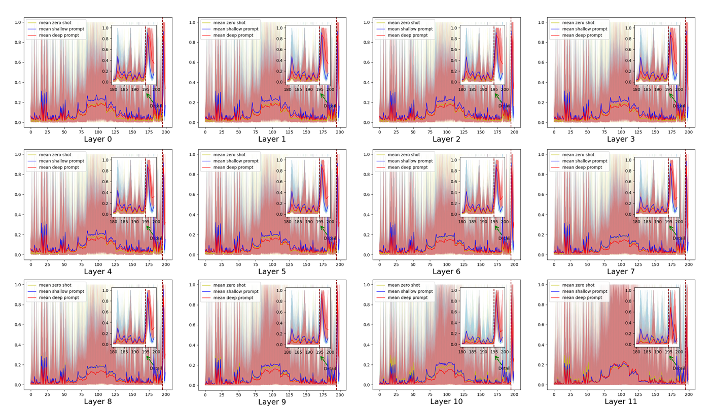
Figure 11: Statistics results on the contribution of each patch of the image branch to the alignment task for the FgvcAircrafat [24] dataset.

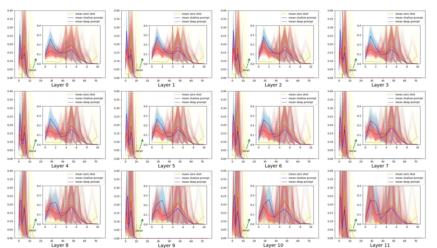
Figure 12: Statistics results on the contribution of each patch of the language branch to the alignment task for the OxfordFlowers [26] dataset.

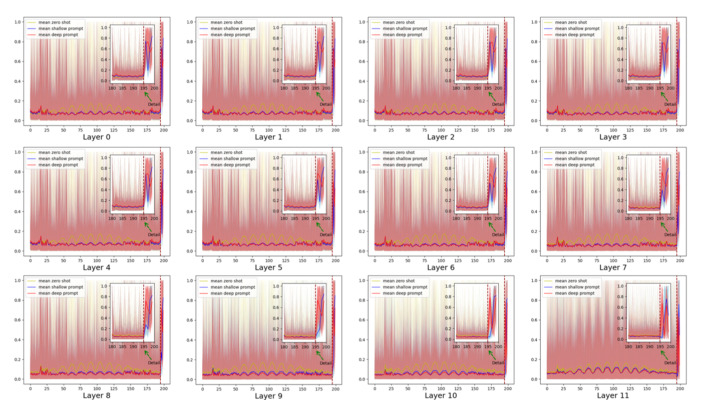
Figure 13: Statistics results on the contribution of each patch of the image branch to the alignment task for the OxfordFlowers [26] dataset.

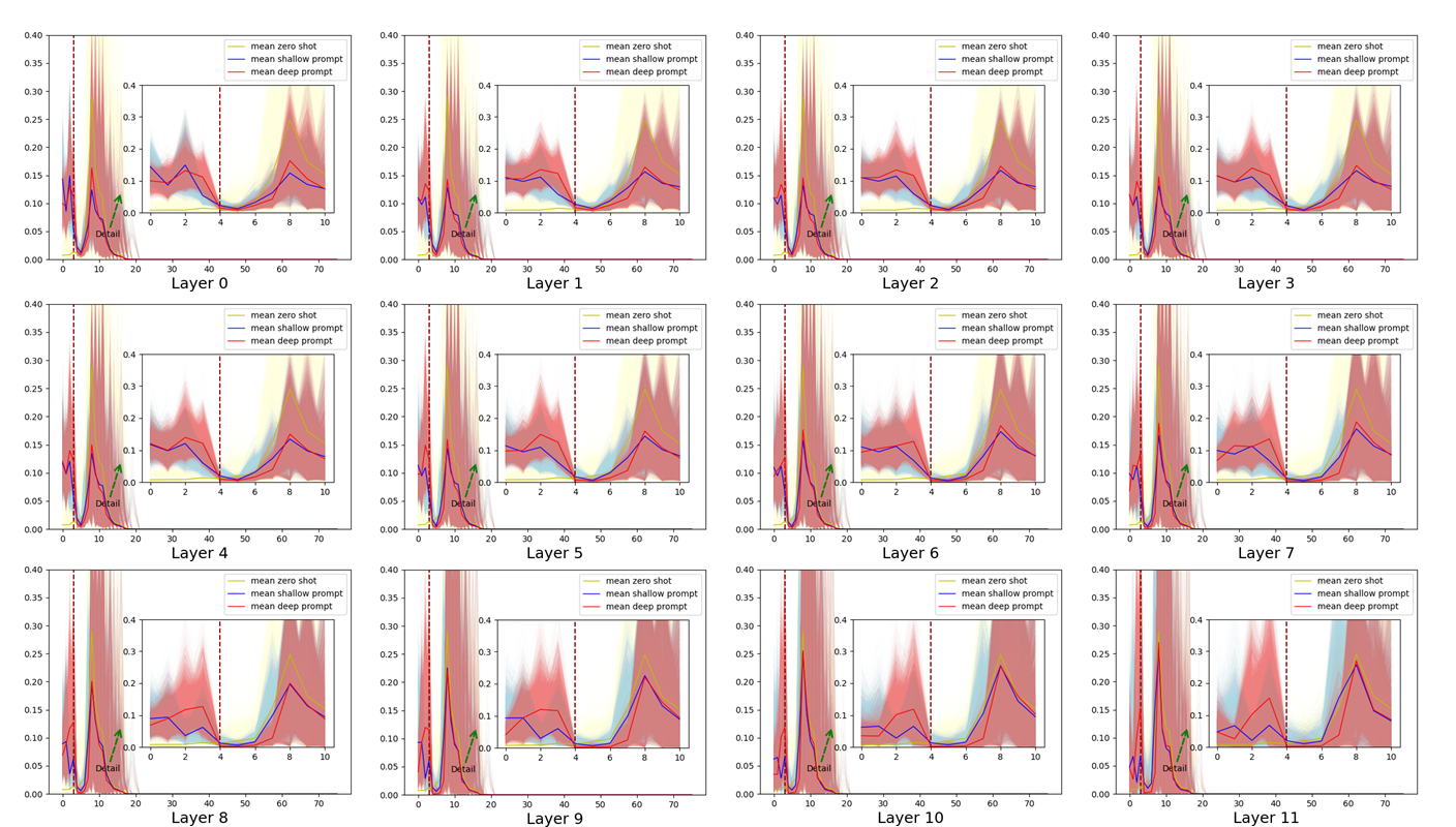
Figure 14: Statistics results on the contribution of each patch of the language branch to the alignment task for the StanfordCars [20] dataset.

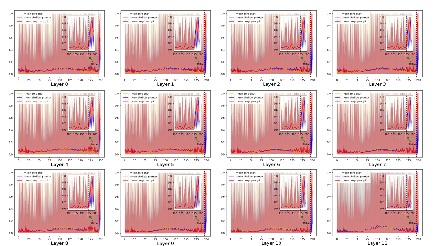
Figure 15: Statistics results on the contribution of each patch of the image branch to the alignment task for the StanfordCars [20] dataset.

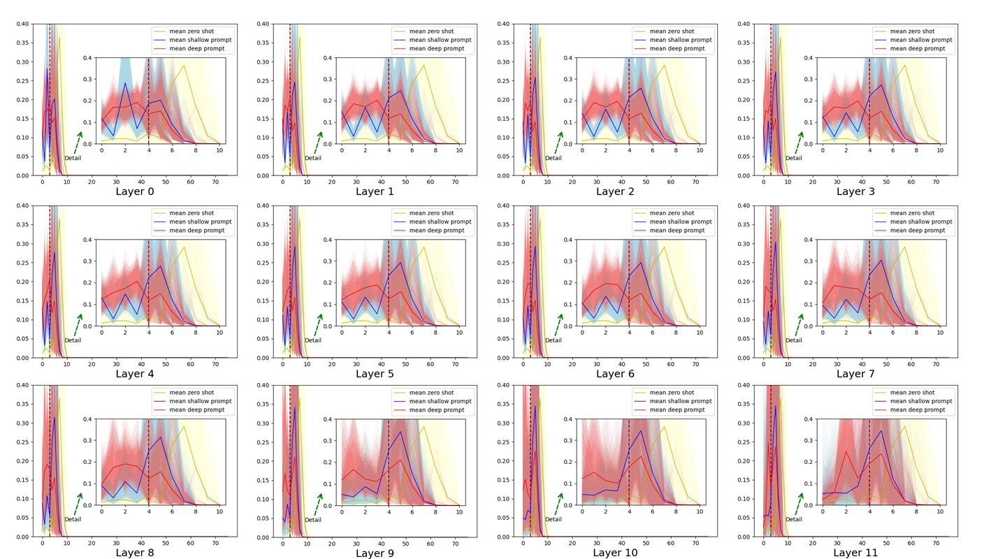
Figure 16: Statistics results on the contribution of each patch of the language branch to the alignment task for the UCF101 [33] dataset.

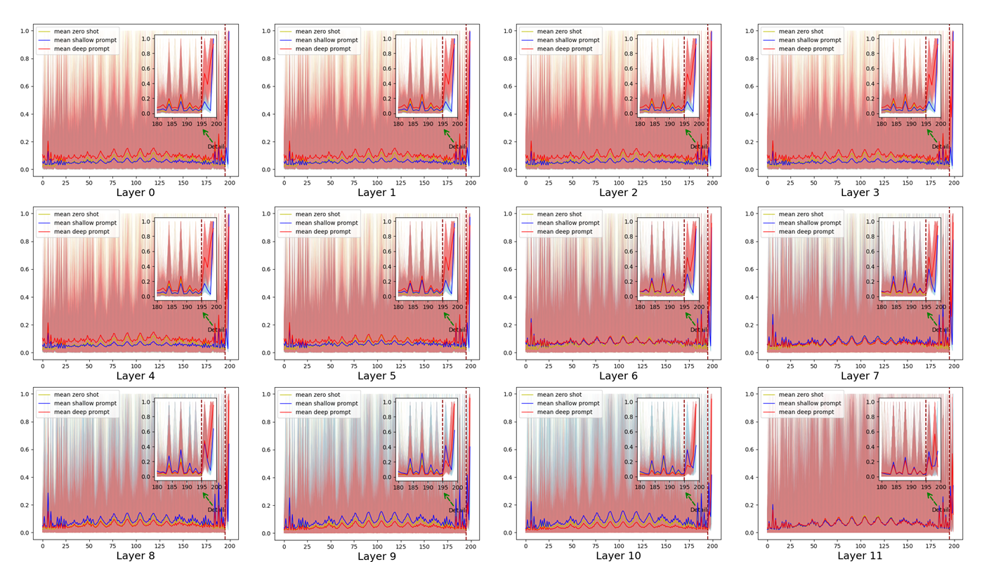
Figure 17: Statistics results on the contribution of each patch of the image branch to the alignment task for the UCF101 [33] dataset.

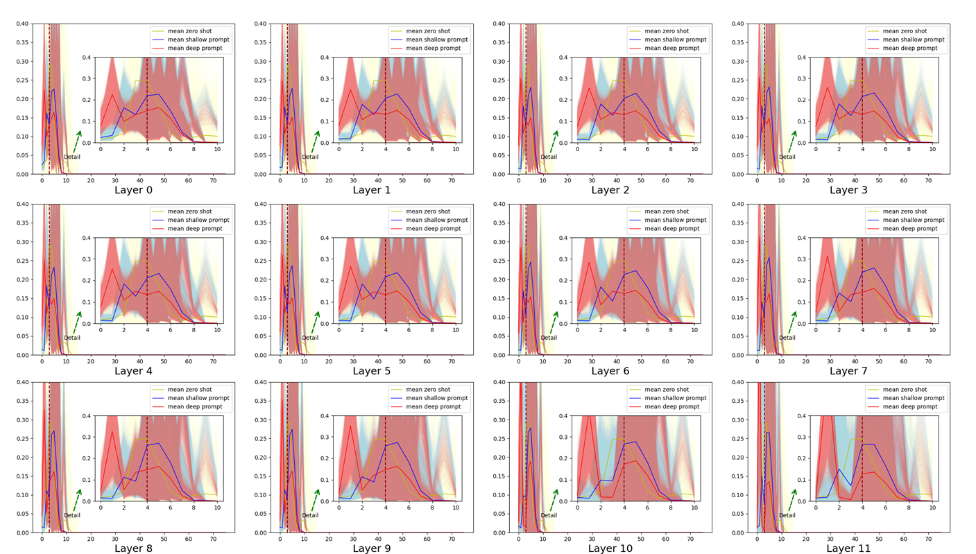
Figure 18: Statistics results on the contribution of each patch of the language branch to the alignment task for the Food101 [2] dataset.

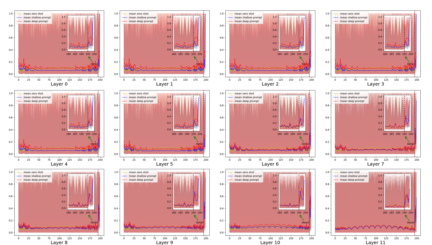
Figure 19: Statistics results on the contribution of each patch of the image branch to the alignment task for the Food101 [2] dataset.

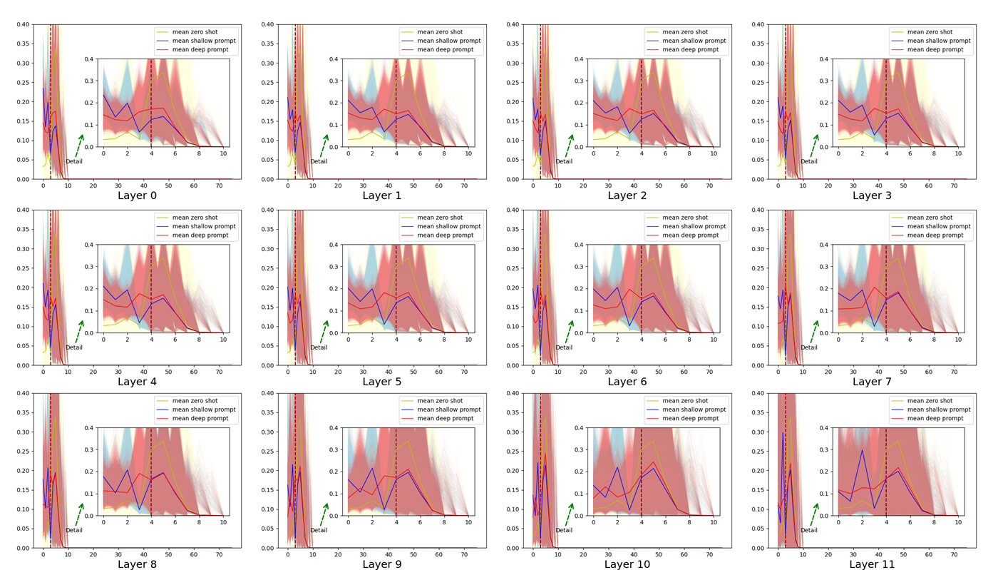
Figure 20: Statistics results on the contribution of each patch of the language branch to the alignment task for the SUN397 [36] dataset.

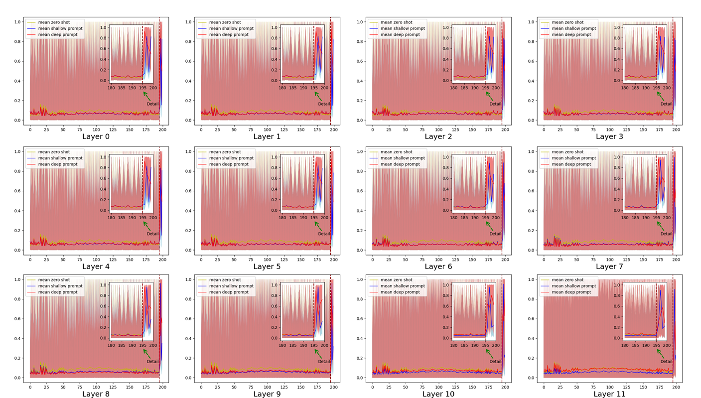
Figure 21: Statistics results on the contribution of each patch of the image branch to the alignment task for the SUN397 [36] dataset.

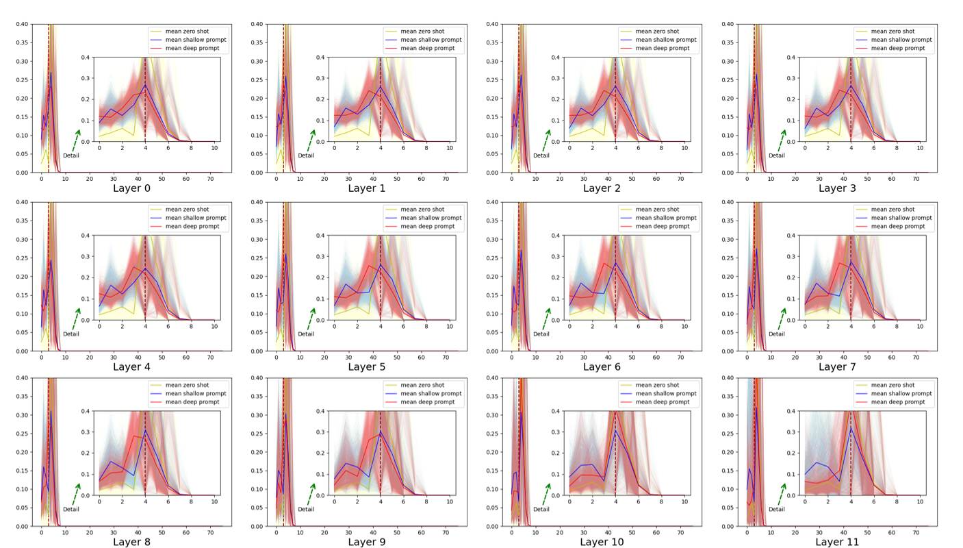
Figure 22: Statistics results on the contribution of each patch of the language branch to the alignment task for the Caltech101 [11] dataset.

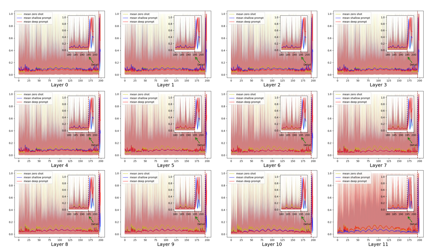
Figure 23: Statistics results on the contribution of each patch of the image branch to the alignment task for the Caltech101 [11] dataset.

References

- Bahng et al. [2022] Hyojin Bahng, Ali Jahanian, Swami Sankaranarayanan, and Phillip Isola. Visual prompting: Modifying pixel space to adapt pre-trained models. arXiv preprint arXiv:2203.17274, 2022.
- Bossard et al. [2014] Lukas Bossard, Matthieu Guillaumin, and Luc Van Gool. Food-101–mining discriminative components with random forests. In ECCV, pages 446–461. Springer, 2014.
- Brown et al. [2020] Tom Brown, Benjamin Mann, Nick Ryder, Melanie Subbiah, Jared D Kaplan, Prafulla Dhariwal, Arvind Neelakantan, Pranav Shyam, Girish Sastry, Amanda Askell, Sandhini Agarwal, Ariel Herbert-Voss, Gretchen Krueger, Tom Henighan, Rewon Child, Aditya Ramesh, Daniel Ziegler, Jeffrey Wu, Clemens Winter, Chris Hesse, Mark Chen, Eric Sigler, Mateusz Litwin, Scott Gray, Benjamin Chess, Jack Clark, Christopher Berner, Sam McCandlish, Alec Radford, Ilya Sutskever, and Dario Amodei. Language models are few-shot learners. In Advances in Neural Information Processing Systems, pages 1877–1901. Curran Associates, Inc., 2020.
- Chefer et al. [2021a] Hila Chefer, Shir Gur, and Lior Wolf. Transformer interpretability beyond attention visualization. In Proceedings of the IEEE/CVF conference on computer vision and pattern recognition, pages 782–791, 2021a.
- Chefer et al. [2021b] Hila Chefer, Shir Gur, and Lior Wolf. Generic attention-model explainability for interpreting bi-modal and encoder-decoder transformers. In Proceedings of the IEEE/CVF International Conference on Computer Vision, pages 397–406, 2021b.
- Chen et al. [2022] Guangyi Chen, Weiran Yao, Xiangchen Song, Xinyue Li, Yongming Rao, and Kun Zhang. Prompt learning with optimal transport for vision-language models. arXiv preprint arXiv:2210.01253, 2022.
- Cimpoi et al. [2014] Mircea Cimpoi, Subhransu Maji, Iasonas Kokkinos, Sammy Mohamed, and Andrea Vedaldi. Describing textures in the wild. In CVPR, pages 3606–3613, 2014.
- Deng et al. [2009] Jia Deng, Wei Dong, Richard Socher, Li-Jia Li, Kai Li, and Li Fei-Fei. Imagenet: A large-scale hierarchical image database. In CVPR, pages 248–255. Ieee, 2009.
- Derakhshani et al. [2022] Mohammad Mahdi Derakhshani, Enrique Sanchez, Adrian Bulat, Victor Guilherme Turrisi da Costa, Cees GM Snoek, Georgios Tzimiropoulos, and Brais Martinez. Variational prompt tuning improves generalization of vision-language models. arXiv preprint arXiv:2210.02390, 2022.
- Ding et al. [2022] Jian Ding, Nan Xue, Gui-Song Xia, and Dengxin Dai. Decoupling zero-shot semantic segmentation. In CVPR, pages 11583–11592, 2022.
- Fei-Fei et al. [2004] Li Fei-Fei, Rob Fergus, and Pietro Perona. Learning generative visual models from few training examples: An incremental bayesian approach tested on 101 object categories. In CVPR Workshop, pages 178–178. IEEE, 2004.
- Gao et al. [2021] Peng Gao, Shijie Geng, Renrui Zhang, Teli Ma, Rongyao Fang, Yongfeng Zhang, Hongsheng Li, and Yu Qiao. Clip-adapter: Better vision-language models with feature adapters. arXiv preprint arXiv:2110.04544, 2021.
- Gu et al. [2021] Xiuye Gu, Tsung-Yi Lin, Weicheng Kuo, and Yin Cui. Open-vocabulary object detection via vision and language knowledge distillation. arXiv preprint arXiv:2104.13921, 2021.
- Helber et al. [2019] Patrick Helber, Benjamin Bischke, Andreas Dengel, and Damian Borth. Eurosat: A novel dataset and deep learning benchmark for land use and land cover classification. J-STARS, 12(7):2217–2226, 2019.
- Huang et al. [2022] Tony Huang, Jack Chu, and Fangyun Wei. Unsupervised prompt learning for vision-language models. arXiv preprint arXiv:2204.03649, 2022.
- Jia et al. [2021] Chao Jia, Yinfei Yang, Ye Xia, Yi-Ting Chen, Zarana Parekh, Hieu Pham, Quoc Le, Yun-Hsuan Sung, Zhen Li, and Tom Duerig. Scaling up visual and vision-language representation learning with noisy text supervision. In ICML, pages 4904–4916. PMLR, 2021.
- Jia et al. [2022] Menglin Jia, Luming Tang, Bor-Chun Chen, Claire Cardie, Serge Belongie, Bharath Hariharan, and Ser-Nam Lim. Visual prompt tuning. In ECCV, 2022.
- Khattak et al. [2023a] Muhammad Uzair Khattak, Hanoona Rasheed, Muhammad Maaz, Salman Khan, and Fahad Shahbaz Khan. Maple: Multi-modal prompt learning. In CVPR, pages 19113–19122, 2023a.
- Khattak et al. [2023b] Muhammad Uzair Khattak, Syed Talal Wasim, Muzammal Naseer, Salman Khan, Ming-Hsuan Yang, and Fahad Shahbaz Khan. Self-regulating prompts: Foundational model adaptation without forgetting. In Proceedings of the IEEE/CVF International Conference on Computer Vision, pages 15190–15200, 2023b.
- Krause et al. [2013] Jonathan Krause, Michael Stark, Jia Deng, and Li Fei-Fei. 3d object representations for fine-grained categorization. In ICCV, pages 554–561, 2013.
- Li et al. [2022] Boyi Li, Kilian Q Weinberger, Serge Belongie, Vladlen Koltun, and Rene Ranftl. Language-driven semantic segmentation. In ICLR, 2022.
- Lu et al. [2022] Yuning Lu, Jianzhuang Liu, Yonggang Zhang, Yajing Liu, and Xinmei Tian. Prompt distribution learning. In CVPR, pages 5206–5215, 2022.
- Maaz et al. [2022] Muhammad Maaz, Hanoona Rasheed, Salman Khan, Fahad Shahbaz Khan, Rao Muhammad Anwer, and Ming-Hsuan Yang. Class-agnostic object detection with multi-modal transformer. In ECCV. Springer, 2022.
- Maji et al. [2013] Subhransu Maji, Esa Rahtu, Juho Kannala, Matthew Blaschko, and Andrea Vedaldi. Fine-grained visual classification of aircraft. arXiv preprint arXiv:1306.5151, 2013.
- Manzoor et al. [2023] Muhammad Arslan Manzoor, Sarah Albarri, Ziting Xian, Zaiqiao Meng, Preslav Nakov, and Shangsong Liang. Multimodality representation learning: A survey on evolution, pretraining and its applications. arXiv preprint arXiv:2302.00389, 2023.
- Nilsback and Zisserman [2008] Maria-Elena Nilsback and Andrew Zisserman. Automated flower classification over a large number of classes. In ICVGIP, pages 722–729. IEEE, 2008.
- Parkhi et al. [2012] Omkar M Parkhi, Andrea Vedaldi, Andrew Zisserman, and CV Jawahar. Cats and dogs. In CVPR, pages 3498–3505. IEEE, 2012.
- Radford et al. [2021] Alec Radford, Jong Wook Kim, Chris Hallacy, Aditya Ramesh, Gabriel Goh, Sandhini Agarwal, Girish Sastry, Amanda Askell, Pamela Mishkin, Jack Clark, et al. Learning transferable visual models from natural language supervision. In ICML, pages 8748–8763. PMLR, 2021.
- Rao et al. [2022] Yongming Rao, Wenliang Zhao, Guangyi Chen, Yansong Tang, Zheng Zhu, Guan Huang, Jie Zhou, and Jiwen Lu. Denseclip: Language-guided dense prediction with context-aware prompting. In CVPR, pages 18082–18091, 2022.
- Rasheed et al. [2022] Hanoona Rasheed, Muhammad Maaz, Muhammad Uzair Khattak, Salman Khan, and Fahad Shahbaz Khan. Bridging the gap between object and image-level representations for open-vocabulary detection. In NeurIPS, 2022.
- Rasheed et al. [2023] Hanoona Rasheed, Muhammad Uzair Khattak, Muhammad Maaz, Salman Khan, and Fahad Shahbaz Khan. Fine-tuned clip models are efficient video learners. In CVPR, pages 6545–6554, 2023.
- Shu et al. [2022] Manli Shu, Weili Nie, De-An Huang, Zhiding Yu, Tom Goldstein, Anima Anandkumar, and Chaowei Xiao. Test-time prompt tuning for zero-shot generalization in vision-language models. arXiv preprint arXiv:2209.07511, 2022.
- Soomro et al. [2012] Khurram Soomro, Amir Roshan Zamir, and Mubarak Shah. Ucf101: A dataset of 101 human actions classes from videos in the wild. arXiv preprint arXiv:1212.0402, 2012.
- Wang et al. [2022a] Zifeng Wang, Zizhao Zhang, Sayna Ebrahimi, Ruoxi Sun, Han Zhang, Chen-Yu Lee, Xiaoqi Ren, Guolong Su, Vincent Perot, Jennifer Dy, et al. Dualprompt: Complementary prompting for rehearsal-free continual learning. In ECCV, 2022a.
- Wang et al. [2022b] Zifeng Wang, Zizhao Zhang, Chen-Yu Lee, Han Zhang, Ruoxi Sun, Xiaoqi Ren, Guolong Su, Vincent Perot, Jennifer Dy, and Tomas Pfister. Learning to prompt for continual learning. In CVPR, pages 139–149, 2022b.
- Xiao et al. [2010] Jianxiong Xiao, James Hays, Krista A Ehinger, Aude Oliva, and Antonio Torralba. Sun database: Large-scale scene recognition from abbey to zoo. In CVPR, pages 3485–3492. IEEE, 2010.
- Yao et al. [2021] Lewei Yao, Runhui Huang, Lu Hou, Guansong Lu, Minzhe Niu, Hang Xu, Xiaodan Liang, Zhenguo Li, Xin Jiang, and Chunjing Xu. Filip: Fine-grained interactive language-image pre-training. arXiv preprint arXiv:2111.07783, 2021.
- Yuan et al. [2021] Lu Yuan, Dongdong Chen, Yi-Ling Chen, Noel Codella, Xiyang Dai, Jianfeng Gao, Houdong Hu, Xuedong Huang, Boxin Li, Chunyuan Li, et al. Florence: A new foundation model for computer vision. arXiv preprint arXiv:2111.11432, 2021.
- Zang et al. [2022] Yuhang Zang, Wei Li, Kaiyang Zhou, Chen Huang, and Chen Change Loy. Open-vocabulary detr with conditional matching. In ECCV, 2022.
- Zhai et al. [2022] Xiaohua Zhai, Xiao Wang, Basil Mustafa, Andreas Steiner, Daniel Keysers, Alexander Kolesnikov, and Lucas Beyer. Lit: Zero-shot transfer with locked-image text tuning. In CVPR, pages 18123–18133, 2022.
- Zhang et al. [2022a] Renrui Zhang, Rongyao Fang, Peng Gao, Wei Zhang, Kunchang Li, Jifeng Dai, Yu Qiao, and Hongsheng Li. Tip-adapter: Training-free clip-adapter for better vision-language modeling. In ECCV, 2022a.
- Zhang et al. [2022b] Yuanhan Zhang, Kaiyang Zhou, and Ziwei Liu. Neural prompt search. arXiv preprint arXiv:2206.04673, 2022b.
- Zhou et al. [2022a] Kaiyang Zhou, Jingkang Yang, Chen Change Loy, and Ziwei Liu. Conditional prompt learning for vision-language models. In CVPR, pages 16816–16825, 2022a.
- Zhou et al. [2022b] Kaiyang Zhou, Jingkang Yang, Chen Change Loy, and Ziwei Liu. Learning to prompt for vision-language models. IJCV, 130(9):2337–2348, 2022b.
- Zhou et al. [2022c] Xingyi Zhou, Rohit Girdhar, Armand Joulin, Philipp Krähenbühl, and Ishan Misra. Detecting twenty-thousand classes using image-level supervision. In ECCV, 2022c.
- Zhu et al. [2022] Beier Zhu, Yulei Niu, Yucheng Han, Yue Wu, and Hanwang Zhang. Prompt-aligned gradient for prompt tuning. arXiv preprint arXiv:2205.14865, 2022.