Learning from Emergence: A Study on Proactively Inhibiting the Monosemantic Neurons of Artificial Neural Networks

Abstract.

Recently, emergence has received widespread attention from the research community along with the success of large language models. Different from the literature, we hypothesize a key factor that highly promotes the performance during the increase of scale: the reduction of monosemantic neurons that can only form one-to-one correlations with specific features. Monosemantic neurons tend to be sparser and have negative impacts on the performance in large models. Inspired by this insight, we propose an intuitive idea to identify monosemantic neurons and inhibit them. However, achieving this goal is a non-trivial task as there is no unified quantitative evaluation metric and simply banning monosemantic neurons does not promote polysemanticity in neural networks. Therefore, we propose to learn from emergence and present a study on proactively inhibiting the monosemantic neurons in this paper. More specifically, we first propose a new metric to measure the monosemanticity of neurons with the guarantee of efficiency for online computation, then introduce a theoretically supported method to suppress monosemantic neurons and proactively promote the ratios of polysemantic neurons in training neural networks. We validate our conjecture that monosemanticity brings about performance change at different model scales on a variety of neural networks and benchmark datasets in different areas, including language, image, and physics simulation tasks. Further experiments validate our analysis and theory regarding the inhibition of monosemanticity.

1. Introduction

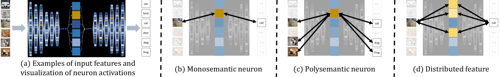
Figure 1. Demonstration of important concepts:(a) A multilayer neuron network for the image classification task. The middle layer is highlighted. (b) A monosemantic neuron (orange) ideally activates for one specific type of feature. (c) A polysemantic neuron activates for multiple features. (d) A distributed feature is classified based on the activation of multiple neurons.

The activity of artificial neural networks diminished for decades before experiencing great success after the 2010s (Krogh, 2008; Krizhevsky et al., 2012). One major difference compared to previous models is the increasing scale. In recent years, large neural networks have much larger scales in terms of datasets, model sizes, and training quantities, which have achieved remarkable results in various fields (Floridi and Chiriatti, 2020; Touvron et al., 2023). Given increasing scales, the performance improvements can usually be estimated under the scaling law (Kaplan et al., 2020), which follows stable but slow increasing trend of power laws (OpenAI, 2023). However, improvements that significantly deviate from estimation occur when the scale increases. Emergence, an intriguing phenomenon in large-scale models, refers to the gradual improvement of model performance before the scale reaching a certain threshold, followed by a rapid enhancement once the threshold is surpassed (Wei et al., 2022). Increasing evidence suggests that the surprises may not arise from new module and architecture designs, but rather from the underlying nature of scale changes (Zhou et al., 2023). A critical question arises: people increase the model scale and get better results, but what has changed underlying the process?

From the perspectives of monosemantic and polysemantic neurons, some pioneer works try to interpret the performance of small and large-scale models, respectively. Through statistical analysis of the relationships between neurons and input features, a neuron is considered monosemantic if it forms a 1-1 correlation with its related input feature (Bau et al., 2020; Elhage et al., 2022) (Figure 1-b). In contrast, polysemantic neurons activate for several features that are weakly correlated (Trenton et al., 2023; Chris et al., 2020; Gabriel et al., 2021; Elhage et al., 2022) (Figure. 1-c). Researchers find that smaller models incur larger errors (Gurnee et al., 2023) when an input’s related monosemantic neuron is disabled. Following the favor of monosemantic neurons from studies on small-scale models, existing works focus on enhancing or extracting monosemanticity (Gurnee et al., 2023; Elhage et al., 2022; Trenton et al., 2023). However, some evidences support that monosemantic neurons are sparser in larger models (Gurnee et al., 2023; Trenton et al., 2023). Those observations imply a positive relationship between the decrease in monosemanticity and the increase in model scale. In other words, monosemanticity could be negatively related to large-scale and good performance. In this paper, inspired by those observations, we propose an important hypothesis that the decrease of monosemantic neurons is a key factor in achieving higher performance as the model scale increases. Figure. 4 in Appx. A shows an example analogy to demonstrate our idea.

Since the research community does not realize the above hypothesis, we rather conclude the current paradigm of training neural networks as a passive process in decreasing monosemantic neurons. This raises an interesting question: can we proactively induce the decrease of monosemantic neurons in artificial neural networks to achieve high performance?

In this paper, we propose to learn from emergence and present a study on proactively inhibiting the monosemantic neurons, which is achieved in two phases:(i) monosemantic neuron detection and (ii) monosemantic neuron inhibition. Unfortunately, it is challenging to design detection and inhibition methods. First, strictly defining monosemantic neurons is still under discussion in quantitative analysis, i.e., detection is impossible without a consensual definition. Besides, existing works (Gurnee et al., 2023; Trenton et al., 2023; Steven et al., 2023a) for detecting the activation degree of neurons introduce extra computation and may suffer from the efficiency issue. Second, we prove that simply prohibiting the activation of monosemantic neurons will intensify the monosemanticity of artificial neural networks. To solve these challenges, we first propose a new metric to measure the monosemanticity of neurons with the guarantee of efficiency for online computation. Then, we identify the drawbacks of simple methods and propose a theoretically supported Reverse Deactivation method to suppress monosemantic neurons and promote the ratios of polysemantic neurons in training neural networks. Our contributions are summarized as follows:

• Inspired by emergence, we propose a novel idea to study the impact of monosemantic and polysemantic neurons on the performance of artificial neural networks. Different from the literature, we propose a hypothesis that monosemanticity could be negatively related to good performance on large-scale models.

• There is no quantitative definition of monosemanticity with high computational efficiency. To effectively detect monosemantic neurons, we propose a new evaluation metric of monosemanticity with a theoretical guarantee on online computation.

• To overcome the inherent drawback of the naive inhibition methods, we propose a theoretically supported reverse deactivation method to suppress monosemantic neurons. It can be integrated as a parameter-free and flexible insertion module, which can adapt to various neural network structures and introduce no computational overhead during testing.

• To validate the effectiveness and generalizability of our method, we conducted tests on various tasks including language, image, and physics simulation. The proposed method MEmeL is applied to milestone models such as Bert, ConvRNN, and different architectures like Transformer, CNN, and RNN. The experimental results demonstrate that MEmeL performs well on different neural networks and corresponding tasks.

2. Preliminary

Given a training set $D=\{(\mathbf{x},\mathbf{y})\}$ of labeled examples, artificial neural networks aim to train a neural network model $f(\mathbf{W};\mathbf{x})$ parameterized by $\mathbf{W}$ so that the predicted output of $\mathbf{x}$ is close to the ground truth $\mathbf{y}$. Under the supervised learning task, we take the cross entropy function $\mathcal{L}(\mathbf{W};D)$ as the example:

(1) $$\min_{\mathbf{W}}\mathcal{L}(\mathbf{W};D)=\min_{\mathbf{W}}-\sum_{(\mathbf{x},\mathbf{y})\in D}\mathbf{y}\log f(\mathbf{W};\mathbf{x}),$$

where $\mathbf{x}=[x_{1},\cdots,x_{d}]\in\mathbb{R}^{d}$ is a $d$-dimensional vector representing the $n$-th input data sample, such as a weather record series covering $d$ days or an image with height $\times$ width $=d$ pixels.

Without loss of generality, let $f(\mathbf{W};\mathbf{x})$ be a $L$-th layer fully connected neural networks (Haykin, 1994). We denote $h_{i}^{\ell}$, $\sigma_{i}^{\ell}(\cdot)$, $z_{i}^{\ell}$ as the input after linear transformation, activation function, and output of the $i$-th hidden unit at $\ell$-th layer, respectively. Then, we may formally define the computation within neurons as follows:

(2) $$h_{j}^{\ell}=\sum_{i}w_{ij}^{\ell}z_{i}^{\ell-1},$$

(3) $$z_{i}^{\ell}=\sigma_{i}^{\ell}(h_{i}^{\ell}),$$

where $z_{i}^{0}\in\mathbf{z}^{0}=\mathbf{x}$, $w_{ij}^{\ell}$ denotes the weight of $i$-th hidden neuron at $(\ell-1)$-th layer to $j$-th hidden neuron at $\ell$-th layer. We use $\mathbf{o}=\mathbf{z}^{L}$ to denote the model output. Existing works on monosemanticity mainly study the layers of values outputted by activation functions (i.e., $\mathbf{z}^{\ell}$). In contrast to other linear layers, these activated values undergo element-wise nonlinearity and are more likely to have independent meanings (Gurnee et al., 2023; Dar et al., 2023). Thus, without loss of generality, we zoom in and study monosemanticity based on one single layer of activated values, e.g., $\mathbf{z}^{\ell}$ in the $\ell$-th layer. Then, $f(\mathbf{W};\mathbf{x})$ can be divided into a frontal model $f_{1}(\cdot)$ and a followed model $f_{2}(\cdot)$ at $\ell$-th layer of output as follows:

(4) $$\mathbf{z}=f_{1}(\mathbf{x})=\sigma^{\ell}(\mathbf{W}^{\ell}(\cdots\sigma^{2}(\mathbf{W}^{2}\sigma^{1}(\mathbf{W}^{1}\mathbf{x}))\cdots)),$$

(5) $$\mathbf{o}=f_{2}(\mathbf{z},\mathbf{x})=\text{Softmax}(\mathbf{W}^{L}\cdots\sigma^{\ell+2}(\mathbf{W}^{\ell+2}\sigma^{\ell+1}(\mathbf{W}^{\ell+1}\mathbf{z}))\cdots),$$

where the frontal model $f_{1}(\cdot)$ takes the original data $\mathbf{x}$ as inputs and delivers output values in $\ell$-th layer $\mathbf{z}$ (with the superscript $\ell$ omitted for simplicity in notation.) As the rest components of the network, the following model $f_{2}(\cdot)$ takes $\mathbf{x}$ and $\mathbf{z}$ and outputs $\mathbf{o}$ (the entire model’s output), and $\mathbf{W}^{\ell}\in\mathbb{R}^{d_{\ell}\times d_{\ell+1}}$ denotes weights of linear transformation from the $\ell$-th layer to the $(\ell+1)$-th layer.

2.1. Activation and Monosemantic

Despite the progress of neural networks and emergence, there is no consensus definition for an “activated” neuron and a “monosemantic” neuron (Elhage et al., 2022). Here we try to summarize an intuitive introduction to describe them.

The Concept of Activation: If an input $\mathbf{x}^{[n]}$ triggers a neuron $z_{i}$ to output a value $f_{1}(\mathbf{x}^{[n]})_{i}$ that deviates “significantly” from the statistical mean (i.e., $\bar{z}_{i}$) , we say that neuron $z_{i}$ is activated by input $\mathbf{x}^{[n]}$. The challenge in defining activation lies in reaching a consensus on the meaning of “significantly”. Instead, we can provide a relative definition as follows. Generally, $i$-th neuron at $\ell$-th layer is considered to be more activated on $\mathbf{x}^{[2]}$ if:

(6) $$\left\|\bar{z}_{i}-(f_{1}(\mathbf{x}^{[1]}))_{i}\right\|<\left\|\bar{z}_{i}-(f_{1}(\mathbf{x}^{[2]}))_{i}\right\|,$$

where $\mathbf{x}^{[{n}]}\in D$ is the ${n}$-th sample in the training set $D$, $\bar{z}_{i}$ is the mean value of $i$-th neuron given all training samples $D$ at $\ell$-th layer, $(f_{1}(\mathbf{x}^{[1]}))_{i}$ denotes the $i$-th output of the frontal model (i.e., $z^{\ell}_{i}$ for $\mathbf{x}^{[1]}$), and $\left\|\cdot\right\|$ is a distance metric. However, while this relative definition is accurate for illustration purposes, it is not concise and is difficult to use for further analysis.

Thus, to give a one-input-wise definition, one may rely on a threshold to define whether a neuron is activated, such as a hard threshold $\tau$. If the deviation of activation value from the mean $\|{\bar{z}_{i}-(f_{1}(\mathbf{x}^{[n]}))_{i}}\|$ exceeds $\tau$, it is generally considered that the neuron is activated. Otherwise, it is in an inactive state. The reason for setting $\tau$ is that neurons will generally have certain fluctuating outputs even for those unrelated different inputs. Unfortunately, setting a universal or adaptive $\tau$ remains to be explored. Therefore, it is also impractical to quantify activation by the threshold.

The Concept of Monosemanticity: However, further illustration for monosemanticity is closely related to a definition of activation that considers only one input at a time. We provide an abstract definition for it: $act(z_{i},\mathbf{x}^{[n]})$, which equals 1 when $z_{i}$ is activated by $\mathbf{x}^{[n]}$, and 0 otherwise. One can use a task-oriented definition as implementation.

To understand neural networks, an important research direction is to correlate neuron activations with human-interpretable features, such as Python and German for language processing; fur and grass for image processing, et al.. Existing works construct feature datasets $\{C_{1},\cdots,C_{m}\}$ for $m$ features, each containing a set of inputs. These feature datasets are specifically designed to partition the inputs $X=\{\mathbf{x}\}$, mathematically:

$$\forall_{i\neq j}C_{i}\cap C_{j}=\emptyset;\bigcup_{i=1}^{m}C_{i}=X.$$

A neuron $z_{i}$ is “monosemantic” if it is only activated on inputs that share a specific feature $C_{j}$, that is:

$$\forall_{\mathbf{x}}act(z_{i},\mathbf{x})=1,\mathbf{x}\in C_{j}$$

However, features are human-defined and vary a lot. In their study, Gurnee et al. (2023) consider about 100 features, while Trenton et al. (2023) study up to $10^{5}$ features to fully capture monosemanticity. Without unified feature datasets, it is also difficult to explicitly formalize the definition of “monosemantic”. More related works are discussed in Appx. B.

Thus, to detect monosemantic neurons, previous studies require manually labeled feature datasets and time-consuming offline computations after model training. To detect and inhibit monosemantic neurons during training, it is necessary to define a lightweight online metric $\phi(\cdot)$ that does not rely on feature datasets, which indicates the level of monosemanticity of a neuron.

2.2. Monosemanticity Inhibition

To achieve the desired output $z$, deep learning models use optimization strategy $\omega$ to update parameters ($\mathbf{W}$), such as minimizing the explicit loss function through gradient descent.

However, to inhibit monosemanticity, there is no related loss function to minimize. In this paper, we achieve this objective in two phases.

Recall that the model $f$ is parameterized by $\mathbf{W}$ and split into a frontal model $f_{1}$ and a followed model $f_{2}$ with respect to the studied layer of neurons $\mathbf{z}$.

Assume that we feed input $\mathbf{x}$ to $f$ and find $z_{i}\in\mathbf{z}$ is monosemantic. By using a well-designed optimization strategy $\omega$, parameters are updated to $\mathbf{W}^{*}$. By feeding the same input $\mathbf{x}$ into the neural network, the frontal model, the followed model, and the layer of neurons are updated to $f_{1}^{*}$, $f_{2}^{*}$, and $\mathbf{z}^{*}$, respectively. We hope that:

• With updated $f_{1}$, neuron $z_{i}$ is less activated for input $\mathbf{x}$. Formally, given old $z_{i}\in\mathbf{z}=f_{1}(\mathbf{x})$ and updated $z_{i}^{*}\in\mathbf{z}^{*}=f_{1}^{*}(\mathbf{x})$, we expect:

  $$\phi(z_{i}^{*})<\phi(z_{i}).$$

• With updated $f_{2}$, the output is still robust when neuron $z_{i}$ is deactivated. Formally, replace $z_{i}$ with a weakly activated value $z_{i}^{\prime}$ (i.e., $\phi(z_{i}^{\prime})<\phi(z_{i})$) to obtain $\mathbf{z}^{\prime}$, we expect the loss $\mathcal{L}$ satisfies:

  $$\mathcal{L}(f_{2}^{*}(\mathbf{z}^{\prime},\mathbf{x}))<\mathcal{L}(f_{2}(\mathbf{z}^{\prime},\mathbf{x})).$$

The two phases (1) prevent the neuron from exclusively serving only one feature type, and (2) prevent this feature modeling from relying solely on one neuron.

3. Methods

As discussed in Sec. 1, the existing neural network training paradigm is a passive process of decreasing monosemantic neurons. To proactively reduce monosemanticity, it is an intuitive solution to detect monosemantic neurons and inhibit them. Unfortunately, achieving these goals is challenging because the monosemanticity measurement does not exist and the simple inhibition method is counterproductive. Therefore, we first propose a new metric to measure the monosemanticity of artificial neurons with the guarantee of computation efficiency, then introduce a theoretically supported inhibition method to suppress monosemantic neurons to proactively reduce the ratios of monosemantic neurons in training artificial neural networks.

3.1. Metric for Monosemanticity

To proactively detect monosemantic neurons, it is important to design a metric that is general for different tasks and efficient to calculate. However, as discussed in Sec. 2, strictly defining “activated” is still under discussion in quantitative analysis (Elhage et al., 2022), which in turn leads to the difficulty of defining “monosemantic”. Although some pioneer works explore the measurement of monosemanticity, these metrics are inflexible for different tasks since they require a predefined and manually labeled feature dataset (Gurnee et al., 2023; Trenton et al., 2023). To address these limitations, we propose a robust metric $\phi(\cdot)$ that can accurately detect monosemantic neurons in this subsection. This metric fulfills two important criteria: (1) generality to make the metric do not rely on any specific dataset, (2) efficiency to enable fast online detection during training.

Intuitively, defining monosemantic neurons mainly requires starting from two principles: high deviation of activation value and low frequency of activation. First, a neuron is considered “activated” when its output value for the current input deviates from the mean value of outputs for all possible inputs. For a monosemantic neuron, its value distribution is more skewed and incurs large deviation (Elhage et al., 2022). Second, each monosemantic neuron only activates when its corresponding feature is inputted, which rarely happens considering the current datasets with steadily growing scales of samples and feature types. Following two principles, we formally define our metric Monosemantic Scale (MS for short) as follows.

Definition 3.1 (Monosemantic Scale).

Given a neuron $z_{i}\in\mathbf{z}$, we denote its historical samples under $m$ inputs $\{\mathbf{x}^{[1]},\mathbf{x}^{[2]},\cdots,\mathbf{x}^{[m]}\}$ as $\{z^{[1]}_{i},z^{[2]}_{i},\cdots,z^{[m]}_{i}\}$ and new value under the $(m+1)$-th input $\mathbf{x}^{[m+1]}$ as $z^{[m+1]}_{i}$. The Monosemantic Scale is defined as:

(7) $$\phi(z^{[m+1]}_{i})=\frac{(z^{[m+1]}_{i}-\bar{z}_{i})^{2}}{S^{2}},$$

where

$$\bar{z}_{i}=\frac{\sum_{j=1}^{m}z^{[j]}_{i}}{m},S^{2}=\frac{\sum_{j=1}^{m}(z^{[j]}_{i}-\bar{z}_{i})^{2}}{m-1},$$

are the sample mean and sample variance, respectively.

In the following contents, we will focus on this single neuron and use $z$ for simplicity.

As shown in Eq. (7), the measurement $\phi(\cdot)$ is proportional to the degree of deviation from the mean. The high deviation of the activation value ensures that the term $(z^{[m+1]}-\bar{z})^{2}$ in $\phi$ can effectively identify neurons with high monosemanticity. Besides, the metric is inversely proportional to the degree of fluctuation because the size of the deviation is also highly correlated with the fluctuation of the activation value on the current data set. Since $\bar{z}_{i}$ is mainly determined by the values when the neuron is deactivated, using the mean as the benchmark for evaluating deviations ensures that the defined neurons with high activation values are rare, i.e., low frequency.

As discussed in Sec. 1 and 2, prior works need to first find the neuron-feature relationships (Gurnee et al., 2023; Trenton et al., 2023) under the manually defined feature data set. Instead, we relax the requirement of discovering corresponding features and eliminate the need for a predefined feature set since we focus on finding monosemantic neurons.

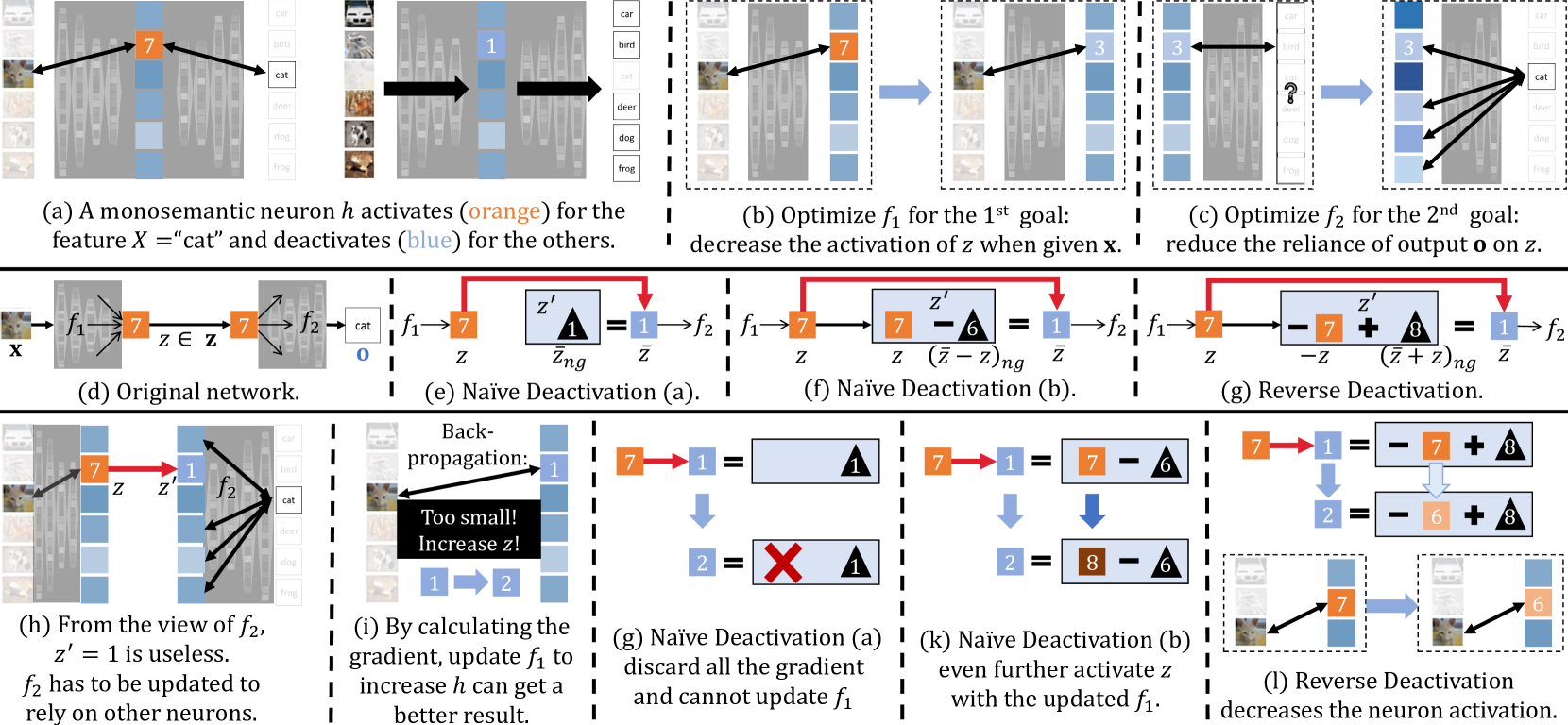
Figure 2. Illustration of problems and solutions to inhibit monosemanticity. (a) A monosemantic neuron $z$ only activates (orange) for the feature “cat” with a high mean value ($=7$). $z$ is deactivated (blue) for other inputs with a small mean value ($\bar{z}=1$). (b) The first goal is to optimize the frontal model $f_{1}$ so that $z$ is less activated given the input “cat”. (c) The second goal is to optimize the followed model $f_{2}$ so that a correct output for “cat” does not solely rely on $z$. (d) Zoom in on the original model at neuron $z$. (e) Naive solution that sets $z^{\prime}$ to a constant 1 without gradient. (f) Naive solution that decreases the value of $z$ to $\bar{z}$ with a constant 6 without gradient. (g) Reverse Deactivation that first reverses $z$ then pushes the output value to $\bar{z}$ by adding a constant 8 without gradient. (h) All the methods can achieve the second goal by outputting a value $\mathcal{V}(z^{\prime})=\bar{z}$ to $f_{2}$. As $\bar{z}$ provides little information, $f_{2}$ must learn to rely on other neurons. (i) When calculating the gradient, $f_{1}$ will find that $z$ is too small and tends to increase it (e.g., from 1 to 2). (j) Naive method (a) cannot update related parameters without gradient. (k) Naive method (b) further increases the underlying $z$ activation (7 to 8). (l) Reverse Deactivation inherently deactivates $z$ (from 7 to 6). When a new batch arrives, the updated $z^{*}$ activates less (=6) for “cat” compared with $z$.

Metric Online Computing Guarantee. It is mandatory to compute the metric $\phi(\cdot)$ to avoid excessive computational burden caused by detecting monosemanticity. As discussed in Sec. 2, pioneer works (e.g., pairwise comparison in Eq. (6)) and other detection methods like probes necessitate training and offline inference for statistical analysis may be costly for online training. Here we show that for each neuron, our proposed MS $\phi(\cdot)$ can be obtained by keeping track of 2 variables in constant time ($O(1)$). Since inputs are typically received in batches (with the number of new samples being greater than 1) during the training of deep learning models, we present the following lemma for training with a batch size of $b$.

Lemma 3.2.

Denote $\mu_{m}$ as the value of the sample mean $\bar{z}$ given $m$ samples, while $\upsilon_{m}$ as the sample variance $S^{2}$. When the $(m+1)^{th}\sim(m+b)^{th}$ samples ${z^{[m+1]},\cdots,z^{[m+b]}}$ come, one can obtain the updated values via:

(8) $$\mu_{m+b} =\frac{m\mu_{m}+b\mu_{b}^{\prime}}{m+b},$$

(9) $$\upsilon_{m+b} =\frac{mb(\mu_{m}-\mu_{b}^{\prime})^{2}}{(m+b-1)(m+b)}+\frac{b\upsilon^{\prime}_{b}+(m-1)\upsilon_{m}}{m+b-1},$$

where $\mu_{b}^{\prime}=\frac{\sum_{i=1}^{b}z_{[m+i]}}{b}$ and $\upsilon^{\prime}_{b}=\frac{\sum_{i=1}^{b}(z_{[m+i]}-\mu^{\prime}_{b})^{2}}{b}$, which is of $O(1)$ time and memory complexity as $b$ is a constant.

The proof is given in Appendix. C.1. In the implementation, we introduce a forgetting mechanism during model updates, where the influence of previous samples should decay. For details, please refer to Algorithm. 1 in Appendix. E.2.

3.2. Inhibition of Monosemanticity

After defining a quantitative metric in Sec. 3.1, it is intuitive to inhibit those monosemantic neurons directly. Unfortunately, simply deactivating monosemantic neurons will intensify the monosemanticity of neural networks. In this subsection, we will first prove the weakness of the native solution in Sec. 3.2.1. To address this unexpected phenomenon, we propose a theoretically supported reverse deactivation method in Sec. 3.2.2.

3.2.1. Naive Deactivation

Recall that given a monosemantic neuron $z$ and an input $\mathbf{x}$ that contains its exclusive feature, we aim to optimize the model in two aspects: (1) decrease the activation level of $z$ when given $\mathbf{x}$ (Figure. 2(b)); and (2) reduce the reliance of output $\mathbf{o}$ on the activation of $z$ (Figure. 2(c)).

Without loss of generality, we focus on the most monosemantic single neuron $z$ in a layer of neurons $\mathbf{z}$. As defined in Sec. 3.1, such a neuron has a large $\phi(z)=(z-\bar{z})^{2}/S^{2}$, which is expected to be inhibited during model optimization. From the perspective of information theory, suppose that the distribution of activation values follows a normal distribution, a neuron provides the least amount of information $I(z)$ when its value equals its statistical mean:

$$\min_{z}[{I(z)}]=\min_{z}[{-\log(P(z))}]=-\log(P(\bar{z})),$$

which is also its most inactive state. $P(\cdot)$ represents the probability density function of values of $z$.

Thus, a straightforward idea to deactivate $z$ is to modify its value to $\bar{z}$. We denote the modified neuron as $z^{\prime}$. One can find two naive solutions to deactivate a neuron:

(10) $$\text{way}(a):\ \ z^{\prime}=\ \bar{z}_{ng},$$

(11) $$\text{way}(b):\ \ z^{\prime}=\ z+(\bar{z}-z)_{ng},$$

where subscript $\cdot_{ng}$ refers to a “no gradient” fixed-value scalar without trainable parameters, compared with $z\in\mathbf{z}=f_{1}(\mathbf{x})$ which is updatable. Two examples are given in Figure. 2(e,f). Both solutions ensure that $f_{2}$ receives an updated $z^{\prime}$, in which the value of $\mathcal{V}(z^{\prime})=\bar{z}$ provides little information. As $z^{\prime}$ is valueless, $f_{2}$ has to adjust its parameter to utilize information from other neurons in $\mathbf{z}$ for good output $\mathbf{o}^{*}=f_{2}^{*}(\mathbf{z}^{\prime},\mathbf{x})$. Such a process achieves our second goal of reducing the dependence of output $\mathbf{o}$ on the activation of $z$ (Figure. 2(l)).

However, neither of the two solutions can achieve the first goal (i.e., training $f_{1}$ to inhibit the activation of $z$ for a single feature). To be more specific, method (a) wastes all the gradient for $f_{1}$ in generating $z$, preventing the related parameters from being updated. Method (b) outputs $\mathcal{V}(z^{\prime})=\bar{z}$ by compensating for the gap. As the model obtains a good result with $z$, by calculating the gradient, $f_{1}$ will be updated to push its output value from $\bar{z}$ to $z$, expressed as $\bar{z}+\delta(z-\bar{z})$, where $\delta>0$ up to the learning rate (Figure. 2(i)). Ironically, the actual output of $z$ is updated to $z+\delta(z-\bar{z})$, deviating from $\bar{z}$ by a factor of $1+\delta$:

$$\frac{z+\delta(z-\bar{z})-\bar{z}}{z-\bar{z}}=1+\delta.$$

Therefore, these two simple solutions either contribute nothing to the deactivation of $z$ or even enhance its activation (Figure. 2(gk)).

After delving deeper into the literature, it is possible that previous researchers also recognized the negative effects of monosemanticity, but they may have discontinued their efforts after obtaining bad results from implementing these naive solutions.

3.2.2. Reversed Deactivation

To address the aforementioned problems, we propose our method called Reversed Deactivation (RD for short). Following the above-mentioned definitions, we replace the original $z$ with $z^{\prime}$ (Figure. 2(f)):

(12) $$z^{\prime}=-z+(\bar{z}+z)_{ng}.$$

Similar to baselines, RD also ensures the second goal of decreasing the dependence of output $\mathbf{o}$ on the activation of $z$. To be more specific, $f_{2}$ receives a value $\mathcal{V}(z^{\prime})=\mathcal{V}({-z+(\overline{z}+z)_{ng}})=\overline{z}$, which provides little information and requires $f_{2}$ to learn the information from other neurons in $\mathbf{z}$ (Figure. 2(h)).

Besides, RD can inhibit the activation level of $z$ when given $\mathbf{x}$. In short, after calculating the gradient, $f_{1}$ will update the trainable parameter to push its output value from $\bar{z}$ to $z$ (Figure. 2(i)). Different from method (b), the gradient on $z$ is reversed. To achieve the same shifted value $\bar{z}+\delta(z-\bar{z})$ mentioned above, an insight into the update can be expressed as:

(13) $$\mathcal{V}(-{z}+(\bar{z}+z)_{ng}) =\bar{z}$$

(14) $$\rightarrow\mathcal{V}(-{(z-\delta(z-\bar{z}))}+(\bar{z}+z)_{ng}) =\bar{z}+\delta(z-\bar{z})$$

The output of $f_{1}$ without post deactivation (i.e., $z-\delta(z-\bar{z})$) is closer to $\bar{z}$ with a factor $1-\delta$:

$$\frac{z-\delta(z-\bar{z})-\bar{z}}{z-\bar{z}}=1-\delta,$$

which achieves deactivation (Figure. 2(j)). The formal and detailed theory is presented in the following lemma.

Lemma 3.3.

Given a trained model $f$ with $2$ continuous derivatives and a Lipschitz continuous gradient, where $f$ achieves a desired output $\mathbf{o}$ with minimal loss $\mathcal{L}(\mathbf{o})$, in which $\textbf{o}=f(\mathbf{x})=f_{2}(f_{1}(\mathbf{x}),\mathbf{x})=f_{2}(\mathbf{z},\mathbf{x})$ for input $\mathbf{x}$ based on its monosemantic neuron $z$ in layer $\mathbf{z}$, suppose that $\mathcal{L}(f_{2}(\cdot))$ monotonically increases with $|z^{\prime}-z|$ for any other value $z^{\prime}$ that replaces $z$. Then, with a sufficiently small learning rate $l$, by updating the model $f$ with gradient descent based on the neuron processed by the RD method, the activation of $z$ on input $\mathbf{x}$ can be inhibited.

The proof is given in Appendix. C.2.

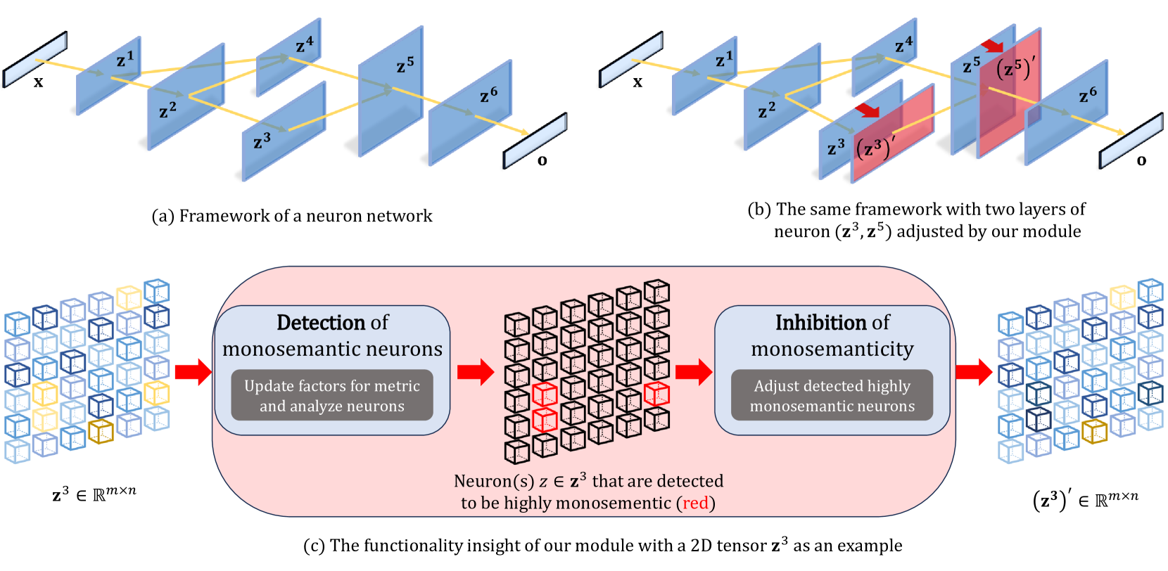
Figure 3. Overview of our method: (a) An arbitrary neural network framework. $\mathbf{x}$ represents the input and $\mathbf{o}$ represents the output. $\mathbf{z}$s represent hidden layers of neurons, and arrows indicate the dependency relationships. (b) Our module is inserted after $\mathbf{z}^{3}$ and $\mathbf{z}^{5}$, requiring no changes to the framework. (c) Details of our module applied to $\mathbf{z}^{5}$. The input neurons are first analyzed using our metric. Once monosemantic neurons are identified, they are inhibited using RD. The resulting processed layer has the same shape as the input.

Additionally, we conduct validation experiments to compare the optimization outputs based on different methods in subsection. 4.3. The results are consistent with the theory and the analysis of naive methods and RD, showing that RD is effective in inhibiting monosemanticity.

3.3. Flexible Plug-in Module

In this subsection, we demonstrate the implementation of our method, which can be inserted after any neuron layer to inhibit its monosemanticity for emergence induction. We name our module Monosemanticity-based Emergence Learning (MEmeL for short) and outline the advantages of MEmeL:

• Adaptivity: Our module is compatible with any design of framework, and no structural changes are needed after inserting it.

• Light weight: No additional trainable parameters are introduced.

The details of MEmeL are displayed in Figure. 3. We present a general framework of a neural network in Figure. 3(a). The output $\mathbf{o}$ is derived from $\mathbf{x}$ based on the layers of neurons $\{\mathbf{z}\}$. Yellow arrows indicate the reliance of neuron layers on each other. Our method can be applied to any layer of neurons, such as $\mathbf{z}^{3}$ and $\mathbf{z}^{5}$ in Figure. 3(b), where the original neurons are adjusted by our modules to inhibit monosemanticity.

Taking $\mathbf{z}^{5}$ as an example (Figure. 3(c)), we first detect monosemantic neurons using our MS metric, as introduced in subsection. 3.1. After identifying these neurons (colored red), we apply our Reverse Deactivation method, as described in subsection. 3.2, to each of them.

For adaptability, our module (i) does not require a specific input format and (ii) outputs $(\mathbf{z}^{5})^{\prime}$ in the same shape as the input $\mathbf{z}^{5}$, ensuring format consistency during data propagation. Thus, no adjustments to the framework are needed to apply our module.

For lightweightness, neither of our two methods introduces any trainable parameters. Additionally, MEmeL focuses on presenting the idea of functionality induction. The methods we propose do not directly decrease monosemanticity during training, but instead induce the model to do so, supported by theoretical analysis. Once we have a well-trained model, the performance is expected to be robust even without induction. Therefore, during testing, the module can be directly removed without incurring any inference overhead. The results of the validation experiments also support our analysis of removing MEmeL during testing. (see Appx. F.1).

Table 1. Results on GLUE Test datasets. We follow the setting of BERT to demonstrate results on 8 datasets and calculate the average score. The scores are F1 scores for QQP and MRPC, Spearman correlations for STS-B, and accuracy scores for the other tasks. All metrics are the larger the better with best results in bold font.

Model	MNLI-(M/MM)	QQP	QNLI	SST-2	CoLA	STS-B	MRPC	RTE	Average
Original	84.6/83.4	71.2	90.5	93.5	52.1	85.8	88.9	66.4	79.6
Naive (a)	84.3/83.6	71.7	90.6	93.8	52.1	85.8	88.2	66.4	79.6
Naive (b)	84.7/84.1	71.6	90.6	93.6	51.8	86.5	87.2	68.0	79.8
MEmeL	84.8/83.9	71.7	90.9	93.6	54.5	86.6	87.6	66.4	80.0
MEmeL-Tune	84.8/83.9	71.7	91.2	93.7	55.7	86.6	89.0	68.1	80.5

The detailed algorithm is provided in the Appendix. D.2. We also apply two simple tricks for implementation: late start and variance compensation, to avoid unstable value fluctuations during the cold start.

Last but not least, we emphasize the proposition of the pipeline for emergence-based learning. Researchers can focus on separable directions: (1) improving the metric to better detect factors related to scale change, and (2) designing factor-oriented solutions for better performance.

4. Experiments

In this section, we first introduce the basic experimental setup in Sec. 4.1, then present the main empirical studies in Sec. 4.2. We show a case study that the proposed Reverse Deactivation is more powerful in inhibition monosematicity than the naive methods in Sec. 4.3. Furthermore, we discuss the potentials and limitations of MEmeL in Sec. 4.4. Note the experiment about the impact of removing MEmeL during test is provided in Appx. F.1 due to the limited space.

4.1. Experimental Setup

Table 2. The experimental results of Swin-Transformer on the ImageNet data and ConvGRU on the data HKO-7. For results on ImageNet-1k dataset, 3 Swin-Transformers pretrained on ImageNet-22k are used as backbones. The metric used is top-1 accuracy, where a higher value indicates better performance. For results on HKO-7 dataset, we initially train a ConvGRU model for 20k steps to create the base model. The metrics used are B-MSE and B-MAE, where a smaller value indicates better performance. The best results are in bold fonts.

Model	Swin-T	Swin-S	Swin-B	B-MAE	B-MSE
Size	28M	50M	88M
Original	80.9	83.2	85.1	1003.41	309.96
Naive (a)	81.0	83.4	84.6	1003.56	309.83
Naive (b)	81.0	83.4	85.1	1003.40	310.13
MEmeL	81.1	83.4	85.1	1003.25	209.94
MEmeL-Tune	81.1	83.5	85.2	998.81	298.16

Table 3. Validation experiments conducted on the Swin-B model. We record the Decrease Ratios and Update Scales of 10k neurons. The model that utilizes our Reverse Deactivation method is compared with those using two Naive methods and the original Swin-B.

Methods	Original	Naive (a)	Naive (b)	Reverse Deactivation
Average Decrease Ratio	0.003%	-0.017%	-0.044%	0.013%
Average Total Update Ratio	0.052%	0.118%	0.161%	0.189%

4.1.1. Data Sets, Base Models, and Tasks

To validate the conjecture of monosemantic neurons, our inhibition method, and corresponding theories, we apply MEmel to milestone models such as Bert, Transformer, and ConvRNN on various tasks (e.g., language, image, and physics simulation), respectively.

• Language Task. We apply MEmeL to the BERT (Pre-training of Deep Bidirectional Transformers) model (Devlin et al., 2019) on the GLUE (General Language Understanding Evaluation) benchmark (Wang et al., 2019). BERT utilizes a transformer architecture and is pretrained on a large corpus of text data. It excels at capturing context and generating high-quality representations of words and sentences. GLUE serves as a benchmark for natural language understanding tasks, encompassing various tasks such as natural language inference, sentiment analysis, and similarity analysis.

• Image Task. We conduct experiments on the Swin-Transformer model (Liu et al., 2021) and ImageNet dataset (Deng et al., 2009). The Swin-Transformer is a transformer model that uses a hierarchical structure and shift-based windows to capture cross-window connections. Our experiment follows their approach, which involves fine-tuning the Swin-Transformer on ImageNet-1K using checkpoints pretrained on ImageNet-22K. ImageNet-1K is a classification benchmark with 1,000 classes, consisting of 1.28 million training images and 50,000 validation images.

• Physics Simulation Task. We apply our MEmeL to the ConvGRU model on the HKO-7 dataset (Shi et al., 2017), which forecasts precipitation based on images of radar echoes (Shi et al., 2015). ConvGRU is a lightweight module that belongs to the ConvRNN class, a milestone structure that combines CNN and RNN to capture spatiotemporal correlations simultaneously. HKO is a large-scale benchmark dataset from the Hong Kong Observatory (HKO), providing high-resolution radar images spanning multiple years. Generally, precipitation forecasting is a challenging task, for both theory-driven and data-driven approaches, as it exhibits complex chaotic dynamics (Xuebin et al., 2017; Wang et al., 2017).

The configuration of above base models generally follow their original settings (see more details in Appx. E.1). The metrics can be found in Appx. E.2. We emphasize that our method is a general module applicable to models of any scale. After applying our module, the effectiveness of MEmeL can be evaluated by comparing it with the original model.

4.1.2. Hyper-parameter Setting

This paper focuses on the performance improvement that is brought by introducing reverse deactivation into milestone models. To fairly validate the effectiveness of the proposed MEmel, we deactivate the neuron with only top-$1$ MS in each batch (recorded as $\rm{MEmeL}$). In other words, we give up the way of determining the number of neurons to be deactivated through hyper-parameter tuning. Therefore, setting may somehow compromise the score improvement, but it preserves fairness. Besides, we also display the results with tuned hyper-parameters (recorded as $\rm{MEmeL-Tune}$). See more details in Appx. E.3.

4.1.3. Implementation

All the codes are implemented in PyTorch (Adam et al., 2017), which is available in the supplementary materials. Our experiment is conducted on 4 V100 GPU cards. Our code are available through the anonymous repo.

4.2. Main Experiment Result

Tab. 1 and Tab. 2 demonstrate the performance of MEmeL incorporated with BERT, Swin-Transformer, and ConvGRU, respectively. The “Original” method denotes the raw model, “Naive (a)” and “Naive (b)” are corresponding to the original model incorporated with naive inhibition methods (see details in Eq. (10)). By comparing the original method and the method enhanced with MEmeL, we can see that the MEmeL (especially MEmeL-Tune) achieves better or comparable results on different tasks, different data sets, and different base models. This validates that neural networks can achieve better results by deactivating monosemantic neurons. By comparing Naive (a), (b) with MEmeL (and MEmeL-Tune), we can easily observe that naive deactivation methods may intensify the monosemanticity of neural networks, which may lead to inferior performance improvement as discussed in Sec. 3.2.1.

4.3. Case Study on Deactivating Monosemantic Neurons

To validate that the monosemanticity is indeed inhibited by our reverse deactivation, we conducted experiments on the ImageNet-1k dataset using the Swin-Transformer model as shown in Tab. 3. We collected 10k samples for 4 different settings, where the modification of $h$ was done using Original (no modification), and two naive methods (a) and (b), and Reverse Deactivation in Sec. 3.2.2.

We feed inputs $\mathbf{x}$ to the model again to check how $z$ is optimized after updating the model with $\mathbf{x}$. The new value is denoted as $z^{\prime}$. Then, the Decrease Ratio represents how the monosemanticity is decreased upon $z$: $\textit{Decrease Ratio}=\left(1-\phi(z^{\prime})/\phi(z)\right)\times 100\%$. Without any modification, monosemanticity showed a slight decrease with a small positive average decrease ratio (0.003%) in the original model. Naive methods (a) and (b) intensify monosemanticity since their decrease ratios are negative, which is consistent with our analysis in Sec. 3.2.1. On the contrary, reverse deactivation has the most significant impact on decreasing monosemanticity (0.013%). But the value is relatively small. That is mainly because the small learning rate ($2\times 10^{-6}$) usually leads to a small update step in training. To provide a clear illustration, we further define the Total Update Ratio as $\textit{Total Update Ratio}=\left|z^{\prime}/z-1\right|\times 100\%$. The scale of modification on $z$ and on $\phi(\cdot)$ is compatible (e.g., 0.013% versus 0.189% for RD). Thus, the small scale of the Decrease Ratio is due to the small learning rate, indicating a stable impact on the inhibition of monosemanticity using our method.

4.4. Potential and Limitation of MEmeL

According to our hypothesis, MEmeL induces the model to accumulate general and abstract functionality instead of monosemanticity for a specific task, which is consistent with the goal of per-taining. Although MEmeL achieves good results during fine-tuning (demonstrated at Main Experiments in Sec. 4.2), the improvement is expected to be even greater when it is applied to the pre-training phase.

The main obstacle is the high computational resource cost required for per-taining. Currently, we have only completed validation on relatively small precipitation forecasting datasets. In Tab. 4, the model pre-trained with MEmeL (P-MEmeL) outperforms the one without it (P-Original). Based on these two models, the same finetuning process is conducted without MEmeL. Using MEmeL during pretraining improves B-MAE by 0.18% and B-MSE by 1.29% (T-MEmeL). In contrast, using MEmeL during finetuning improves B-MAE by 0.02% B-MSE by 0.01% (MEmeL in Table. 2). The results validate our hypothesis.

Table 4. Validation experiments conducted on the HKO-7 dataset. In addition, we pretrain a ConvGRU model for 20k steps using MEmeL, labeled as “P-MEmeL”. The “P-Original” model is pretrained based on the original model and is used in the main experiment. Based on these two models, we perform finetuning for 2k steps using the original model, labeled as “T-MEmeL” and “T-Original”, respectively. The metrics used for evaluation were B-MSE and B-MAE, where a smaller value indicates better performance. The best results are shown in bold fonts.

Model	B-MAE	B-MSE
P-Original	1004.25	311.54
P-MEmeL	1000.98	306.67
T-Original	1003.41	309.96
T-MEmeL	1001.56	305.96

5. Conclusion

Different from the literature, we hypothesize a key factor that highly promote the performance of large neural networks: the reduction of monosemantic neurons. There is no unified quantitative evaluation metric and simply banning monosemantic neurons does not promote polysemanticity in neural networks. Therefore, we propose to learn from emergence and present a study on proactively inhibiting the monosemantic neurons in this paper. More specifically, we first propose a new metric to measure the monosemanticity of neurons with the guarantee of efficiency for online computation, then introduce a theoretically supported method to suppress monosemantic neurons and proactively promote the ratios of polysemantic neurons in training neural networks. We validate our conjecture that monosemanticity brings about performance change at different model scales on a variety of neural networks and benchmark datasets in different areas, including language, image, and physics simulation tasks. Further experiments validate our analysis and theory regarding the inhibition of monosemanticity.

Unfortunately, extending this research to very large data sets or models (e.g., large language models) is appealing yet impossible for research departments due to limited resources. Therefore, we are trying to find ways to extend this paper to extremely large models trained on large data sets as future work.

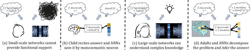
Figure 4. An analogy example to demonstrate our motivation: (a) ANNs could be similar to biological brains. Small-scale networks (both biological and artificial) cannot support complex functionality. (b) To solve a difficult problem that requires complex reasoning, pupils rely on rote memorization, while ANNs store QA pairs using monosemantic neurons as key-value pairs. (c) Large-scale networks can learn and master solving skills related to integration. (d) Adults and large-scale ANNs are capable of decomposing features and inferring answers using complex neuron circuits. This ability reduces reliance on rote memory and monosemanticity.

Appendix A An Example Analogy that Helps Illustrate Our Motivation

We display an example with neuroscience analogy to better illustrate our motivation. For more relationships with neuroscience, see discussions in subsection. G.1.

From the perspective of scale differences, when the model is small, the limited number of neurons makes it difficult to abstract and analyze the input, and to provide functional support for integrating a large amount of scattered information (Figure. 4(a)). To achieve good results, neurons tend to specialize in certain features, resulting in stronger monosemanticity (Figure. 4(b)).

We can analogize a small neural network to a developing brain of a pupil, memorizing question-answer pairs. Constructing monosemantic neurons is easier to achieve good results in complex tasks (such as accurately answering ten complex integration problems), compared to expecting the pupil to understand the solving steps and reason the results by themselves. (Not to mention that providing datasets with solving steps is very rare in neural network training, and small models struggle to automatically acquire reasoning abilities based solely on input-output pairs through simple gradient descent).

Similarly, we can analogize large models to adults, allowing them to learn and master solving skills related to integration (Figure. 4(c)). This is because adults have accumulated knowledge and have a more mature brain development, similar to the huge training volume and parameter size of large models. In this process, adults gradually reduce the reliance on rote memorization and improve their reasoning abilities for new problems (Figure. 4(d)). This can explain why large models have fewer monosemantic neurons and stronger generalization abilities in complex tasks.

To utilize this in model optimization, one issue is that existing large models are passive in decreasing monosemanticity, which can be likened to students lacking systematic education. Large models gradually reduce monosemanticity by accumulating training data, similar to students acquiring skills through extensive learning rather than rote memorization, and good guidance can help students improve faster. This leads us to our question: Can we proactively guide the reduction of monosemantic neurons to improve model performance?

Ideally, models will improve regardless of their scales. This is because large models also have the potential to decrease monosemanticity, resulting in better results.

Appendix B Related Works

B.1. Artificial Neural Networks and the Increasing Scale

Since S and Walter (1943) first modeled a simple neural network, ANN has been investigated under a scale of several layers in the last century (LeCun et al., 1989; Yann et al., 1995). With improvements in hardware, deeper models can be supported. AlexNet, which uses 8 layers for image classification, achieved excellent performance in the 2012 ImageNet challenge (Krizhevsky et al., 2012). Later on, deeper models such as Inception and VGG increased the scale to tens and hundreds of layers (Szegedy et al., 2015; Simonyan and Zisserman, 2015). The design of critical modules, such as ResNet, also plays a crucial role in ensuring the stability of model training when increasing the depth (He et al., 2016).

After the Transformer was proposed and validated as effective in various areas (Vaswani et al., 2017), both its scale and performance have seen significant growth over the years (Devlin et al., 2019; Liu et al., 2021). In recent years, architectures based on the Transformer have achieved great success at extremely large scales (Floridi and Chiriatti, 2020; Touvron et al., 2023). Investigating the underlying effective properties created by the increase in scale is a highly demanded research direction.

B.2. Mechanistic Interpretability

With the improved performance of neural networks, their black-box nature raises more questions than it answers. To gain a better understanding of and diagnose neural networks, researchers seek mechanistic interpretability (Räuker et al., 2022). They study individual components to understand their functionality and usage, such as neurons for identifying dogs and cars (Chris et al., 2020). As Transformer models demonstrate their superiority in various domains, there is an increasing focus on their interpretability. Geva et al. (2021) propose that the feed-forward layers of Transformers function as key-value pairs. Dar et al. (2023) extend this mapping to the embedding space. Although the complexity greatly increases with larger models, the success of these models attracts researchers who strive to find interpretability in the vast sea of neurons (Gurnee et al., 2023; Trenton et al., 2023; Steven et al., 2023b). In their work, Elhage et al. (2022) introduce the softmax linear unit to create monosemantic models. Additionally, Gurnee et al. (2023) modify the sparse probe by using multiple heads to classify neurons with decreasing monosemanticity. Trenton et al. (2023) construct more powerful and complex probes to construct mappings between neurons and features. While the desire to decompose and understand everything is appealing (e.g., achieving monosententicity), it may conflict with the progress of intelligence.

B.3. Debate on the Existence of Emergence

Note that Schaeffer et al. (2023) states that “emergent abilities appear due to the researcher’s choice of metric rather than due to fundamental changes in models with scale”. Here we point out that their finding does not diminish the value of our finding, but instead partially coincides with our idea:

• Though evaluation metrics can be smooth and well-designed, models are improved based on training data. However, solving hard and realistic problems via advanced AI involves more and more data with poorly labeled or even without labels. Emergence learning is demanded to find and boost the underlying ability accumulation of models, which diminishes the correctness of individual answers and focuses on the potential knowledge learning brought by scale changes.

• To observe the accumulated ability of the model on these hard problems, we need smooth and mild metrics. Such metrics may not be available for challenging problems in the future, where the research would be like roaming at deep night. Factors discovered through Emergence Learning can help validate the potential improvement of models and enlighten the darkness.

Appendix C Proof of Sec. 3

C.1. Proof of Lemma. 3.2

Proof.

Recall that we define:

$$\mu_{m}=\frac{\sum_{i=1}^{m}z^{[i]}}{m},\mu_{b}^{\prime}=\frac{\sum_{i=1}^{b}z^{[m+i]}}{b}.$$

We have:

(15) $$\mu_{m+b} =\frac{\sum_{i=1}^{m+b}z^{[i]}}{m+b}$$

(16) $$=\frac{\sum_{i=1}^{m}z^{[i]}+\sum_{i=1}^{b}z^{[m+i]}}{m+b}$$

(17) $$=\frac{m\mu_{m}+b\mu^{\prime}_{b}}{m+b}.$$

Besides, we define:

$$\upsilon_{m}=\frac{\sum_{i=1}^{m}(z^{[i]}-\mu_{m})^{2}}{m-1},\upsilon^{\prime}_{b}=\frac{\sum_{i=1}^{b}(z^{[m+i]}-\mu^{\prime}_{b})^{2}}{b}.$$

Then we have:

(18) $$\upsilon_{m+b}= \frac{\sum_{i=1}^{m+b}(z^{[i]}-\mu_{m+b})^{2}}{m+b-1}=\frac{\sum_{i=1}^{m+b}(z^{[i]}-\frac{m\mu_{m}+b\mu^{\prime}_{b}}{m+b})^{2}}{m+b-1}$$

(19) $$= \frac{\sum_{i=1}^{b}(z^{[m+i]}-\frac{m\mu_{m}+b\mu^{\prime}_{b}}{m+b})^{2}+\sum_{i=1}^{m}(z^{[i]}-\frac{m\mu_{m}+b\mu^{\prime}_{b}}{m+b})^{2}}{m+b-1}$$

(20) $$= \frac{\sum_{i=1}^{b}\left[z^{[m+i]}-\mu^{\prime}_{b}-\frac{m(\mu_{m}-\mu^{\prime}_{b})}{m+b}\right]^{2}+\sum_{i=1}^{m}\left[z^{[i]}-\mu_{m}+\frac{b(\mu_{m}-\mu^{\prime}_{b})}{m+b}\right]^{2}}{m+b-1}$$

(21) $$= \frac{b\left(\frac{m(\mu_{m}-\mu_{b}^{\prime})}{m+b}\right)^{2}+\sum_{i=1}^{b}\left(h_{(i+m)}-\mu^{\prime}_{b}\right)^{2}-\sum_{i=1}^{b}\left[2(z^{[m+i]}-\mu^{\prime}_{b})\frac{m(\mu_{m}-\mu_{b}^{\prime})}{m+b}\right]}{m+b-1}$$

(22) $$+\frac{m\left(\frac{b(\mu_{m}-\mu_{b}^{\prime})}{m+b}\right)^{2}+\sum_{i=1}^{m}\left(z^{[i]}-\mu_{m}\right)^{2}+\sum_{i=1}^{m}\left[2(z^{[i]}-\mu_{m})\frac{b(\mu_{m}-\mu_{b}^{\prime})}{m+b}\right]}{m+b-1}$$

(23) $$= \frac{mb^{2}(\mu_{m}-\mu_{b}^{\prime})^{2}+bm^{2}(\mu_{m}-\mu_{b}^{\prime})^{2}}{(m+b-1)(m+b)^{2}}+\frac{\sum_{i=1}^{b}\left(z^{[m+i]}-\mu_{b}^{\prime}\right)^{2}-0+(m-1)\upsilon_{m}+0}{m+b-1}$$

(24) $$= \frac{mb(\mu_{m}-\mu_{b}^{\prime})^{2}}{(m+b-1)(m+b)}+\frac{b\upsilon^{\prime}_{b}+(m-1)\upsilon_{m}}{m+b-1},$$

where the third terms in Equation. (21) and Equation. (22) equal to zero as $\sum_{i=1}^{b}(z^{[m+i]}-\mu^{\prime}_{b})=\sum_{i=1}^{b}(z^{[m+i]})-b\mu^{\prime}_{b}=0,\sum_{i=1}^{m}(z^{[i]}-\mu_{m})=\sum_{i=1}^{m}(z^{[i]})-m\mu_{m}=0$ and other terms are constant factors. ∎

C.2. Proof and Discussion of Lemma. 3.3

Proof.

Recall that based on Reversed Deactivation, our gradient flow originates from the following equations:

(25) $$\mathbf{o}^{\prime}= f_{2}(\mathbf{z}^{\prime},\mathbf{x})=f_{2}([-z+(z+\bar{z})_{ng},\mathbf{z}^{-},\mathbf{x}]),$$

(26) $$\mathbf{z}= [z,\mathbf{z}^{-}]=f_{1}(\mathbf{x}),$$

where $\cdot_{ng}$ denotes “no gradient” scalar and ${\mathbf{z}^{-}}\subset\mathbf{z}$ are the neurons in $\mathbf{z}$ except $z$.

Though a bit of abusing the symbol, to give a clearer representation for gradient update, we use $z$ to refer to the neuron, $z_{a}$ refers to its activation value which leads to an ideal $\mathbf{o}$. $z_{o}=z_{a}$ as the value of $z$ before processed by RD, $z^{*}$ for the value updated after gradient descent. We still use $\bar{z}$ as the mean value of $z$ and represent the difference between $z$ and $\bar{z}$ as an updating variable $t=z-\bar{z}$. Note that except $z$ and $t$, other definitions in this paragraph are untrainable scalars.

Here we focusing on $z-$related parts of Equation. (25) and (26). We denote parameters of $f_{1}$ as $\theta\in\mathbf{W}$ and rewrite Equation. (26) for gradient calculation and parameter update:

(27) $$z= g(\theta)+\bar{h}$$

(28) $$\Rightarrow t= g(\theta),$$

where $g$ is $z$-related functions of $f_{1}$.

Here we fix other states and focus on the interaction between $z$, $\theta$, and loss $\mathcal{L}(\mathbf{o}^{\prime})$. We can calculate the gradient for $\theta$:

(29) $$\nabla\mathcal{L}(\theta)= \frac{\partial{\mathcal{L}(\mathbf{o}^{\prime})}}{\partial\theta}$$

(30) $$= \frac{\partial{\mathcal{L}(f_{2}(\mathbf{z}^{\prime}))}}{\partial t}\frac{\partial t}{\partial\theta}$$

(31) $$= \frac{\partial{\mathcal{L}(f_{2}(\mathbf{z}^{\prime}))}}{\partial(z^{\prime}-z_{a})}\frac{\partial(z^{\prime}-z_{a})}{\partial t}\frac{\partial t}{\partial\theta}$$

(32) $$= -\nabla f(\delta)\nabla g(\theta),$$

where $\frac{\partial t}{\partial\theta}=\nabla g(\theta)$ as the gradient of Equation. (28) and $\frac{\partial(z^{\prime}-z_{a})}{\partial t}=\frac{\partial(-z+z_{a}+\bar{z}-z_{a})}{\partial(z-\bar{z})}=-1$. $\nabla f(\delta)$ denotes $\frac{\partial{\mathcal{L}(f_{2}(\mathbf{z}^{\prime}))}}{\partial(z^{\prime}-z_{a})}.$ According to our assumption that $f(\delta)$ the monotonically increases with $|z^{\prime}-z_{a}|$, $\nabla f(\delta)\geq 0$ when $z^{\prime}\geq z_{a}$ so that $z^{\prime}-z_{a}=|z^{\prime}-z_{a}|$, which means $\bar{z}\geq z_{a}$ and $t\leq 0$. Also, we can derive that $t\geq 0$ when $\nabla f(\delta)\leq 0$.

With gradient descent of learning rate $l$, we will update parameter $\theta$ as:

(33) $$\theta^{*}\leftarrow\theta-l\nabla\mathcal{L}(\theta)=\theta+l\nabla f(\delta)\nabla g(\theta)$$

By updating the parameter, we can express the updated $z$ with a variation on the multivariate Taylor expansion:

(34) $$z^{*}= g(\theta^{*})$$

(35) $$= g(\theta)+l\nabla g(\theta)^{T}\nabla f(\delta)\nabla g(\theta)+l^{2}\frac{1}{2}(\nabla\mathcal{L}(\theta))^{T}\nabla^{2}g(\theta^{\prime})(\nabla\mathcal{L}(\theta)),$$

where $\theta^{*}$ is the updated parameter and $\theta^{\prime}$ is between $\theta$ and $\theta^{*}$.

When $\nabla f(\delta)\geq 0$, we have

(36) $$z^{*}-z_{o}= l\nabla g(\theta)^{T}\nabla f(\delta)\nabla g(\theta)+\frac{l^{2}}{2}(\nabla\mathcal{L}(\theta))^{T}\nabla^{2}g(\theta^{\prime})(\nabla\mathcal{L}(\theta))$$

(37) $$= l(d_{1}+\frac{l}{2}d_{2}),$$

which is greater than 0 when $d_{2}\geq 0,l>0$ or $d_{2}<0,0<l<\frac{2d_{1}}{-d_{2}}$, where $d_{1}=\nabla f(\delta)||\nabla g(\theta)||^{2}$ and $d_{2}=(\nabla\mathcal{L}(\theta))^{T}\nabla^{2}g(\theta^{\prime})(\nabla\mathcal{L}(\theta))$. As $t=z-\bar{z}<0$ under $\nabla f(\delta)\geq 0$, the activation value is smaller than the mean $\bar{h}$. Note that after the update, $z^{*}>z_{o}$. With a small enough learning rate $l$ (i.e., $<\frac{2d_{1}}{-d_{2}}$), $z^{*}$ will be updated towards $\bar{h}$ and deactivated (i.e., $\bar{h}>z^{*}>z_{o}$)

When $\nabla f(\delta)\leq 0$, we have

(38) $$z^{*}-z_{o}= l\nabla g(\theta)^{T}\nabla f(\delta)\nabla g(\theta)+\frac{l^{2}}{2}(\nabla\mathcal{L}(\theta))^{T}\nabla^{2}g(\theta^{\prime})(\nabla\mathcal{L}(\theta))$$

(39) $$\leq l\nabla f(\delta)||g(\theta)||^{2}+\frac{l^{2}L}{2}||\nabla g(\theta)||^{2},$$

(40) $$= l(\nabla f(\delta)+l\frac{L}{2})||\nabla g(\theta)||^{2}$$

where Equation. (40) is valid as $g$ is the $z$-related part of model $f$ and has a Lipschitz continuous gradient. Equation. (40) is smaller than 0 when learning rate $0<l<(-\nabla f(\delta))\frac{2}{L}$, which ensures that updated output $z^{*}$ is smaller than original activated value $z_{o}$, and thus close to $\bar{z}$ as $t=z-\bar{z}\geq 0$. Together with the case when $\nabla f(\delta)\geq 0$, we show that $z$ is always pushed to mean $\bar{z}$ and deactivated.

∎

We point out that the loss function $\mathcal{L}(\mathbf{o})$ does not always strictly increase with the deviation from $z$ (i.e., $|z^{\prime}-z|$) in neural networks. This is due to the presence of local optima, where increasing deviation from $z$ may actually lead to a smaller loss. Fortunately, in the case of a monosemantic neuron, the output is strongly influenced by $z$ and exhibits less nonlinearity, aligning more closely with the assumption.

Appendix D Implementation Details

D.1. Implementation Details of MS $\phi$

During training, the model is continuously updated. However, samples from the early stages become outdated, and more importance should be given to the new samples. To address this, we introduce a forget step ($n_{f}$) and keep track of the current training steps ($c_{t}$). Once $c_{t}\geq n_{f}$, we update the sample mean and variance by replacing the number of samples from $m$ to $b\cdot n_{f}$. This reduces the influence of previous samples. Both variable updating and mean and variance computation have a complexity of $O(1)$.

Algorithm 1 Monosementicity Scale Computing with Needed Variables

  Input: new batch of values $\left\{\mathbf{z}^{[m+1]},\mathbf{z}^{[m+2]},\cdots,\mathbf{z}^{[m+b]}\right\}$ of the neuron.

  Local Variables: forget step $n_{f}$, current step $c_{t}$, current sample mean $\mu_{m}$ and variance $\upsilon_{m}$

  Calculate the MS for each input value $z\in\mathbf{z}$: $\phi(z^{[m+i]})=(z^{[m+i]}-\mu_{m})^{2}/\upsilon_{m}$ for $i\in[1,b]$.

  Calculate $\mu_{b}^{\prime}=\frac{1}{b}\sum_{i=1}^{b}z^{[m+i]}$ and $\upsilon^{\prime}_{b}=\frac{1}{b}\sum_{i=1}^{b}(z^{[m+i]}-\mu^{\prime}_{b})^{2}$.

  if $c_{t}<n_{f}$ then

     $\mu_{m+b}=\frac{m\mu_{m}+b\mu^{\prime}_{b}}{m+b},$ $\upsilon_{m+b}=\frac{mb(\mu_{m}-\mu_{b}^{\prime})^{2}}{(m+b-1)(m+b)}+\frac{b\upsilon^{\prime}_{b}+(m-1)\upsilon_{m}}{m+b-1}$

  else

     $\mu_{m+b}=\frac{n_{f}\mu_{m}+\mu^{\prime}_{b}}{n_{f}+1},$ $\upsilon_{m+b}=\frac{n_{f}(\mu_{m}-\mu_{b}^{\prime})^{2}}{(n_{f}+1-1/b)(n_{f}+1)}+\frac{\upsilon^{\prime}_{b}+(n_{f}-1/b)\upsilon_{m}}{n_{f}+1-1/b}$

  end if

  RETURN: Monosementicity Scale of inputs $\phi({\mathbf{h}})$

Algorithm 2 Monosementicity-based Emergence Learning

  Input: Values of $n$ neurons with batchsize $b$: $\mathbf{z}=\{\{z_{i}^{[j]}\}_{j=1}^{b}\}_{i=1}^{n}$.

  Local Variables: late start step $l_{s}$, current step $c_{t}$, current sample mean $\{{\mu_{i}}_{m}\}_{i=1}^{n}$ and variance $\{{\upsilon_{i}}_{m}\}_{i=1}^{n}$

  if $c_{t}<l_{s}$ then

     Calculate the MS for each input value

$$\phi(h_{i}^{[m+j]})=\frac{(h_{i}^{[m+j]}-{\mu_{i}}_{m})^{2}}{{\upsilon_{i}}_{m}+\epsilon\sum_{k=1}^{n}{\upsilon_{k}}_{m}/n}\text{ for }i\in[1,n],j\in[1,b].$$

     Select values with high $\phi$, adjust each of them according to MD. Replacing the original ones in $\mathbf{z}$ to form output $\mathbf{z}^{\prime}$.

  else

     $\mathbf{z}^{\prime}=\mathbf{z}$

  end if

  Update sample mean $\{{\mu_{i}}_{m}\}_{i=1}^{n}$ and variance $\{{\upsilon_{i}}_{m}\}_{i=1}^{n}$ using Algorithm. 1.

  RETURN: Adjusted layer of neurons $\mathbf{z}^{\prime}$

D.2. Implementation Details of MEmeL

As described in Algorithm. 1, the statistical variables are calculated online. However, due to the limited number of samples at the beginning of training, the estimation can be unstable. Additionally, if the estimation of $S^{2}$ is extremely small, it may cause overflow during calculation. To improve the robustness of training, we introduce a late start step $l_{s}$ and a variance compensation in the denominator of the metric calculation in Equation. (7). As outlined in Algorithm. 2, when a batch of data arrives, we only update neurons with RD if the current step is greater than $l_{s}$. The calculation of MS is also adjusted by incorporating the mean of variances of other neurons, weighted by a small value $\epsilon$ to prevent overflow.

Appendix E Experiment Setting

E.1. Configuration of Base Models

For the language task, we insert 4 MEemL layers after the 4 middle Attention layers of BERT-base (12 in total). Since MEemL does not introduce any additional parameters, we can directly use their checkpoint after pretraining to finetune. The finetuning setting is the same as BERT for fairness, where each task is trained with a batch size of 32 and 3 epochs over the data for all GLUE tasks. For each task, we selected the best fine-tuning learning rate ($l\in\{5e-5,4e-5,3e-5,2e-5\}$) on the validation dataset (DEV). Baseline results are from Table.1 in BERT (Devlin et al., 2019).

For the image classification task, we also insert 4 MEemL layers after the 4 middle Attention layers for each model. The training is conducted on ImageNet-1k for 30 epochs using pretrained checkpoints on ImageNet-22k. The settings are directly adopted from their scripts, except for the number of GPU cards. Baseline results are collected by running checkpoints from the github of Swin-Transformer with some updates.

For the precipitation task, we insert 6 MEemL lay- ers after the hidden states of each ConvGRU module. The training is conducted on the HKO-7 dataset (Shi et al., 2017) of radar images with a granularity of $120\times 120$, which are centered in Hong Kong. These radar images cover a timespan from 2009 to 2015 and are captured every 6 minutes. The original rainfall intensity is mapped to a scale of [0, 255], forming a regression task. The pretraining settings are the same with theirs, optimizing for 20k steps. Based on that, we conduct 2k more steps funetuning to obtain the final output.

E.2. Metrics

Here we list the metrics used in the experiments.

• The Accuracy: With the statistic of True Positive (TP), False Positive (FP), True Negative (TN), and False Negative (FN), Accuracy can be derived as $\frac{\text{TP+TN}}{\text{TP+TN+FN+FN}}$.

• The F1 score:

  $$F1=\frac{{2\cdot\text{{Precision}}\cdot\text{{Recall}}}}{{\text{{Precision}}+\text{{Recall}}}},$$

  where Precision is calculated as $\frac{\text{TP}}{\text{TP+FP}}$ and Recall refers to $\frac{\text{TP}}{\text{TP+FN}}$.

• The Spearman correlations:

  $$\rho=\frac{\sum_{i}(x_{i}-\bar{x})(y_{i}-\bar{y})}{\sqrt{\sum_{i}(x_{i}-\bar{x})^{2}\sum_{i}(y_{i}-\bar{y})^{2}}},$$

  where $[x_{1},x_{2},\cdots]$ and $[y_{1},y_{2},\cdots]$ are two sequences.

• The B-MSE and B-MAE (The balanced mean square error and balanced mean absolute error):

  $$\text{B-MSE}=\frac{1}{D}\sum_{m\in M}w(m)(m-\hat{m})^{2},$$

  $$\text{B-MAE}=\frac{1}{D}\sum_{m\in M}w(m)|m-\hat{m}|,$$

  where $M\in\mathrm{R}^{T\times H\times W}$ is the radar intensity map to be predicted with $D=T\times H\times W$ pixels. For each pixel with intensity $m$, $\hat{m}$ is the prediction output and $w(m)$ is a weight to enhance the performance on heavy rainfall:

  $$w(m)=\begin{cases}\begin{array}[]{cc}1,&m<2\\ 2,&2\leqslant m<5\\ 5,&5\leqslant m<10\\ 10,&10\leqslant m<30\\ 30,&m\geqslant 30\end{array}&\end{cases}$$

E.3. Parameter Searching over Inhibition Level of Monosemanticity

As mentioned above, to ensure fairness, we apply the minimal scale of inhibition, wherein only the most monosemantic neuron is selected and deactivated for each sample. However, we can also adjust the inhibition scale in each step by introducing a factor $\Delta$. By unifying the two naive methods and our reverse deactivation, we obtain the following function:

$$z^{\prime}=-\Delta\cdot z+(\bar{z}+\Delta\cdot z)_{ng}.$$

Our reverse deactivation (RD) is a special case when $\Delta=1$, while the two naive methods can be obtained with $\Delta=0$ and -1. It can be easily proven that for any $\Delta>0$, the modification can deactivate neuron $z$ according to Lemma 3.3, and a larger $\Delta$ corresponds to a more aggressive deactivation. Therefore, we search for the number of neurons $n_{n}$ to deactivate in a single step and the scale of deactivation $\Delta$ for the best performance. We select the best model from the search space: $n_{n}\in\{1,5,10,50,100\}$ and $\Delta\in\{1,5,10,50,100\}$.

Table 5. Validation results on GLUE Test datasets. The settings are the same with Table. 1. All metrics are the larger the better with best results in bold font.

Model	MNLI-(M/MM)	QQP	QNLI	SST-2	CoLA	STS-B	MRPC	RTE	Average
MEmeL	84.8/83.9	71.7	90.9	93.6	54.5	86.6	87.6	66.4	80.0
MEmeL-T	84.9/83.7	71.5	90.5	93.9	52.1	85.9	88.7	68.1	79.9

Table 6. Validation results on ImageNet-1k dataset. See Table. 2 for detailed settings. The metric is the higher the better. The best results are indicated in bold font.

Model	Swin-T	Swin-S	Swin-B
Size	28M	50M	88M
MEmeL	81.1	83.4	85.1
MEmeL-T	81.1	83.5	85.1

Table 7. Results on HKO-7 dataset. The settings are the same with Table. 2. The metrics are the smaller the better with the best results in bold fonts.

Model	B-MAE	B-MSE
MEmeL	1003.25	309.94
MEmeL-T	1002.46	309.52

Appendix F More Experiments

F.1. The Impact of Removing MEmeL During Test

Recall that in subsection 3.3, we emphasize the lightness of our MEmeL. It aims to induce models to reduce monosemanticity during training and can be removed during testing. Here, we conduct experiments to enable MEmeL during testing, which are expected to have similar results compared to the results displayed in the main experiments (see Section 4.2). These models are labeled with the postfix “-T” (e.g., MEmeL-T for MEmeL as the base model) while keeping other experimental settings unchanged.

The results are displayed in Table. 5, Table. 6, and Table. 7 for GLUE, ImageNet, and HKO-7 datasets, respectively. The best results are shown in bold fonts. The performance differences for the two settings are very close on all three tasks, indicating a stable performance when tested without the induction of MEmeL. Interestingly, on GLUE datasets, the performance when using MEmeL during testing is much more fluctuated. It would be valuable to study the dynamics of MEmeL in more depth as future work.

Appendix G Discussions

G.1. Biological View of Neuron Connection

Monosemanticity and polysemanticity are inherent mappings between neurons, where decreasing monosemanticity encourages the construction of complex mappings instead of exclusive connections. With a similar functionality, in neuroscience, “synaptic” enables information transmission between neurons (Hasson et al., 2020; Thomas et al., 2017). In view of the evolution of the brain, the increase of neuron activity is positively correlated to the increase of the amount of synaptic (M and S, 2015). Besides, compared with chimpanzees, humans significantly have more synaptics for information transmission (A et al., 2012).

However, the connections of artificial neurons are fixed during design. In contrast, the connection relationships of biological neurons are observable, which can serve as a reference to study the monosemanticity of AI neurons in large-scale models.

G.2. Brain-inspired ANN design

Researchers have developed various methods for incorporating biological knowledge into ANNs (G, 2008; Samuel et al., 2023). For example, to guide the design of ANNs, Spiking Neural Networks (SNNs) draw inspiration from the way neurons communicate in the brain, where information is encoded in the timing of spikes or action potentials (CW et al., 2000). This spike-based communication enables SNNs to potentially achieve greater efficiency and better biological plausibility. In optimizing ANNs, Eligibility Propagation combines traditional error backpropagation with biologically plausible learning rules (Bellec et al., 2020). This approach updates the model by calculating an eligibility trace for each synapse and measuring its contribution to the neuron.

These methods tend to help ANN by focusing on the functionality and mechanism of biological neurons, whereas EmeL emphasizes the importance of scale as an angle of improvement.

G.3. Difference from Traditional Normalizations

Previous normalizations have focused on the interaction between neurons in a layer, whereas our metric is based on the behavior of each individual neuron. For example, a neuron could be activated at 0 and deactivated at 2, which would be considered outstanding for normalization, as it consistently outputs a large value. One can better understand the importance of its 0-value through monosemantic analysis.

G.4. On the Selection of Benchmark and Experimental Settings

Currently, middle- to large-scale models typically follow a pretrain-finetune training procedure, such as Bert. Pretraining is usually conducted on multiple datasets to learn general abilities like feature extraction. After pretraining, the model is finetuned for a specific task, which may sacrifice its general ability in favor of better performance.

Intuitively, to achieve the best result, a model should be trained in the following way: (i) use MEmeL during pretraining to decrease monosemanticity and increase the general ability, and (ii) exclude MEmeL during finetuning on a specific task to allow for an increase in monosemanticity and achieve better results. To illustrate, pretraining is similar to a student accumulating knowledge from multiple courses, starting from elementary school to university, while finetuning is akin to preparing for the GRE exam. Monosemanticity is similar to rote memorization, where memorizing questions and answers during courses does not help improve the GRE score, but it is useful when studying for the exam.

However, validating the idea and performing pretraining is much more computationally expensive compared to finetuning, especially for large models. For instance, using the naive method to pretrain LLAMA2-7B based on our A800 is estimated to cost over $$450k$ and over 5800 GPU-days (Touvron et al., 2023) with our preliminary test. Emergence occurs primarily near $10^{22}$ FLOPs and costs more than 10500 GPU-days (Wei et al., 2022). Conducting corresponding validation experiments is impossible for most researchers without the assistance of top companies.

Under such an arms race on GPUs, our experiments explore our resources to first validate the generality and effectiveness of our methods. Though finetuning may not fully utilize the capabilities of MEmeL, our main experiments demonstrate that finetuning with MEmeL is powerful enough to improve results. Additionally, on the precipitation forecasting task with a smaller scale, we conduct pretraining with MEmeL and observe a significant improvement compared to finetuning. The details are provided in subsection. 4.3. This finding supports our idea that compared to finetuning, pretraining can leverage the strengths of MEmeL better.

G.5. Potential Directions of Emergence Learning

Wei et al. (2022) raise the concept of emergence in AI models and point out that the explanation for emergence is still under investigation. They discuss the opinion that AI models can be seen as compressors and explain emergence as a result of the accumulation to compress world knowledge. In this aspect, decreasing monosemanticity encourages models to compress knowledge rather than storing knowledge that compromises generality.

G.6. Future Work of Partially Decreasing Monosemanticity

Increasing monosemanticity can be beneficial in some areas where precise memorization is necessary. It is important to study the impact of monosemanticity on different tasks and inhibit or increase it according to the analysis. A complex task could also be broken down into smaller steps, each with its own preference for monosemanticity.

For example, when asking a model to imitate the author of “Sapiens: A Brief History of Humankind” and write a preface from scratch, the model should accurately identify Harari as the author through a key-value style memorization and then reproduce the tone in the output with the necessary reasoning ability.

References

- (1)
- A et al. (2012) Spocter Muhammad A, Hopkins William D, Barks Sarah K, Bianchi Serena, Hehmeyer Abigail E, Anderson Sarah M, Stimpson Cheryl D, Fobbs Archibald J, Hof Patrick R, and Sherwood Chet C. 2012. Neuropil distribution in the cerebral cortex differs between humans and chimpanzees. Journal of comparative neurology 520, 13 (2012), 2917–2929.
- Adam et al. (2017) Paszke Adam, Gross Sam, Chintala Soumith, Chanan Gregory, Yang Edward, DeVito Zachary, Lin Zeming, Desmaison Alban, Antiga Luca, and Lerer Adam. 2017. Automatic differentiation in PyTorch. (2017).
- Bau et al. (2020) David Bau, Jun-Yan Zhu, Hendrik Strobelt, Àgata Lapedriza, Bolei Zhou, and Antonio Torralba. 2020. Understanding the role of individual units in a deep neural network. Proc. Natl. Acad. Sci. USA 117, 48 (2020), 30071–30078.
- Bellec et al. (2020) Guillaume Bellec, Franz Scherr, Anand Subramoney, Elias Hajek, Darjan Salaj, Robert Legenstein, and Wolfgang Maass. 2020. A solution to the learning dilemma for recurrent networks of spiking neurons. Nature communications 11, 1 (2020), 3625.
- Chris et al. (2020) Olah Chris, Cammarata Nick, Schubert Ludwig, Goh Gabriel, Petrov Michael, and Carter Shan. 2020. Zoom in: An introduction to circuits. Distill 5, 3 (2020), e00024–001.
- CW et al. (2000) Van Rossum Mark CW, Bi Guo Qiang, and Turrigiano Gina G. 2000. Stable Hebbian learning from spike timing-dependent plasticity. Journal of neuroscience 20, 23 (2000), 8812–8821.
- Dar et al. (2023) Guy Dar, Mor Geva, Ankit Gupta, and Jonathan Berant. 2023. Analyzing Transformers in Embedding Space. In ACL (1). Association for Computational Linguistics, 16124–16170.
- Deng et al. (2009) Jia Deng, Wei Dong, Richard Socher, Li-Jia Li, Kai Li, and Li Fei-Fei. 2009. ImageNet: A large-scale hierarchical image database. In CVPR. IEEE Computer Society, 248–255.
- Devlin et al. (2019) Jacob Devlin, Ming-Wei Chang, Kenton Lee, and Kristina Toutanova. 2019. BERT: Pre-training of Deep Bidirectional Transformers for Language Understanding. In NAACL-HLT (1). Association for Computational Linguistics, 4171–4186.
- Elhage et al. (2022) Nelson Elhage, Tristan Hume, Catherine Olsson, Neel Nanda, Tom Henighan, Scott Johnston, Sheer El Showk, Nicholas Joseph, Nova DasSarma, Ben Mann, Danny Hernandez, Amanda Askell, Kamal Ndousse, Andy Jones, Dawn Drain, Anna Chen, Yuntao Bai, Deep Ganguli, Liane Lovitt, Zac Hatfield-Dodds, Jackson Kernion, Tom Conerly, Shauna Kravec, Stanislav Fort, Saurav Kadavath, Josh Jacobson, Eli Tran-Johnson, Jared Kaplan, Jack Clark, Tom Brown, Sam McCandlish, Dario Amodei, and Christopher Olah. 2022. Softmax Linear Units. Transformer Circuits Thread (2022).
- Floridi and Chiriatti (2020) Luciano Floridi and Massimo Chiriatti. 2020. GPT-3: Its Nature, Scope, Limits, and Consequences. Minds Mach. 30, 4 (2020), 681–694.
- G (2008) Turrigiano Gina G. 2008. The self-tuning neuron: synaptic scaling of excitatory synapses. Cell 135, 3 (2008), 422–435.
- Gabriel et al. (2021) Goh Gabriel, Cammarata Nick, Voss Chelsea, Carter Shan, Petrov Michael, Schubert Ludwig, Radford Alec, and Olah Chris. 2021. Multimodal neurons in artificial neural networks. Distill 6, 3 (2021), e30.
- Geva et al. (2021) Mor Geva, Roei Schuster, Jonathan Berant, and Omer Levy. 2021. Transformer Feed-Forward Layers Are Key-Value Memories. In EMNLP (1). Association for Computational Linguistics, 5484–5495.
- Gurnee et al. (2023) Wes Gurnee, Neel Nanda, Matthew Pauly, Katherine Harvey, Dmitrii Troitskii, and Dimitris Bertsimas. 2023. Finding Neurons in a Haystack: Case Studies with Sparse Probing. CoRR abs/2305.01610 (2023).
- Hasson et al. (2020) Uri Hasson, Samuel A Nastase, and Ariel Goldstein. 2020. Direct fit to nature: an evolutionary perspective on biological and artificial neural networks. Neuron 105, 3 (2020), 416–434.
- Haykin (1994) Simon Haykin. 1994. Neural networks: a comprehensive foundation. Prentice Hall PTR.
- He et al. (2016) Kaiming He, Xiangyu Zhang, Shaoqing Ren, and Jian Sun. 2016. Deep Residual Learning for Image Recognition. In CVPR. IEEE Computer Society, 770–778.
- Kaplan et al. (2020) Jared Kaplan, Sam McCandlish, Tom Henighan, Tom B. Brown, Benjamin Chess, Rewon Child, Scott Gray, Alec Radford, Jeffrey Wu, and Dario Amodei. 2020. Scaling Laws for Neural Language Models. CoRR abs/2001.08361 (2020).
- Krizhevsky et al. (2012) Alex Krizhevsky, Ilya Sutskever, and Geoffrey E. Hinton. 2012. ImageNet Classification with Deep Convolutional Neural Networks. In NIPS. 1106–1114.
- Krogh (2008) Anders Krogh. 2008. What are artificial neural networks? Nature biotechnology 26, 2 (2008), 195–197.
- LeCun et al. (1989) Yann LeCun, Bernhard E. Boser, John S. Denker, Donnie Henderson, Richard E. Howard, Wayne E. Hubbard, and Lawrence D. Jackel. 1989. Backpropagation Applied to Handwritten Zip Code Recognition. Neural Comput. 1, 4 (1989), 541–551.
- Liu et al. (2021) Ze Liu, Yutong Lin, Yue Cao, Han Hu, Yixuan Wei, Zheng Zhang, Stephen Lin, and Baining Guo. 2021. Swin Transformer: Hierarchical Vision Transformer using Shifted Windows. In ICCV. IEEE, 9992–10002.
- M and S (2015) Gash Don M and Deane Andrew S. 2015. Neuron-based heredity and human evolution. Frontiers in neuroscience 9 (2015), 209.
- OpenAI (2023) OpenAI. 2023. GPT-4 Technical Report. CoRR abs/2303.08774 (2023).
- Räuker et al. (2022) Tilman Räuker, Anson Ho, Stephen Casper, and Dylan Hadfield-Menell. 2022. Toward Transparent AI: A Survey on Interpreting the Inner Structures of Deep Neural Networks. CoRR abs/2207.13243 (2022).
- S and Walter (1943) McCulloch Warren S and Pitts Walter. 1943. A logical calculus of the ideas immanent in nervous activity. The bulletin of mathematical biophysics 5 (1943), 115–133.
- Samuel et al. (2023) Schmidgall Samuel, Achterberg Jascha, Miconi Thomas, Kirsch Louis, Ziaei Rojin, Hajiseyedrazi S, and Eshraghian Jason. 2023. Brain-inspired learning in artificial neural networks: a review. arXiv preprint arXiv:2305.11252 (2023).
- Schaeffer et al. (2023) Rylan Schaeffer, Brando Miranda, and Sanmi Koyejo. 2023. Are Emergent Abilities of Large Language Models a Mirage? CoRR abs/2304.15004 (2023).
- Shi et al. (2015) Xingjian Shi, Zhourong Chen, Hao Wang, Dit-Yan Yeung, Wai-Kin Wong, and Wang-chun Woo. 2015. Convolutional LSTM Network: A Machine Learning Approach for Precipitation Nowcasting. In NIPS. 802–810.
- Shi et al. (2017) Xingjian Shi, Zhihan Gao, Leonard Lausen, Hao Wang, Dit-Yan Yeung, Wai-Kin Wong, and Wang-chun Woo. 2017. Deep Learning for Precipitation Nowcasting: A Benchmark and A New Model. In NIPS. 5617–5627.
- Simonyan and Zisserman (2015) Karen Simonyan and Andrew Zisserman. 2015. Very Deep Convolutional Networks for Large-Scale Image Recognition. In ICLR.
- Steven et al. (2023a) Bills Steven, Cammarata Nick, Mossing Dan, Tillman Henk, Gao Leo, Goh Gabriel, Sutskever Ilya, Leike Jan, Wu Jeff, and Saunders William. 2023a. Language models can explain neurons in language models. URL https://openaipublic. blob. core. windows. net/neuron-explainer/paper/index. html.(Date accessed: 14.05. 2023) (2023).
- Steven et al. (2023b) Bills Steven, Cammarata Nick, Mossing Dan, Tillman Henk, Gao Leo, Goh Gabriel, Sutskever Ilya, Leike Jan, Wu Jeff, and Saunders William. 2023b. Language models can explain neurons in language models. URL https://openaipublic. blob. core. windows. net/neuron-explainer/paper/index. html.(Date accessed: 14.05. 2023) (2023).
- Szegedy et al. (2015) Christian Szegedy, Wei Liu, Yangqing Jia, Pierre Sermanet, Scott E. Reed, Dragomir Anguelov, Dumitru Erhan, Vincent Vanhoucke, and Andrew Rabinovich. 2015. Going deeper with convolutions. In CVPR. IEEE Computer Society, 1–9.
- Thomas et al. (2017) Biederer Thomas, Kaeser Pascal S, and Blanpied Thomas A. 2017. Transcellular nanoalignment of synaptic function. Neuron 96, 3 (2017), 680–696.
- Touvron et al. (2023) Hugo Touvron, Louis Martin, Kevin Stone, Peter Albert, Amjad Almahairi, Yasmine Babaei, Nikolay Bashlykov, Soumya Batra, Prajjwal Bhargava, Shruti Bhosale, Dan Bikel, Lukas Blecher, Cristian Canton-Ferrer, Moya Chen, Guillem Cucurull, David Esiobu, Jude Fernandes, Jeremy Fu, Wenyin Fu, Brian Fuller, Cynthia Gao, Vedanuj Goswami, Naman Goyal, Anthony Hartshorn, Saghar Hosseini, Rui Hou, Hakan Inan, Marcin Kardas, Viktor Kerkez, Madian Khabsa, Isabel Kloumann, Artem Korenev, Punit Singh Koura, Marie-Anne Lachaux, Thibaut Lavril, Jenya Lee, Diana Liskovich, Yinghai Lu, Yuning Mao, Xavier Martinet, Todor Mihaylov, Pushkar Mishra, Igor Molybog, Yixin Nie, Andrew Poulton, Jeremy Reizenstein, Rashi Rungta, Kalyan Saladi, Alan Schelten, Ruan Silva, Eric Michael Smith, Ranjan Subramanian, Xiaoqing Ellen Tan, Binh Tang, Ross Taylor, Adina Williams, Jian Xiang Kuan, Puxin Xu, Zheng Yan, Iliyan Zarov, Yuchen Zhang, Angela Fan, Melanie Kambadur, Sharan Narang, Aurélien Rodriguez, Robert Stojnic, Sergey Edunov, and Thomas Scialom. 2023. Llama 2: Open Foundation and Fine-Tuned Chat Models. CoRR abs/2307.09288 (2023).
- Trenton et al. (2023) Bricken Trenton, Templeton Adly, Batson Joshua, Chen Brian, Jermyn Adam, Conerly Tom, Turner Nick, Anil Cem, Denison Carson, Askell Amanda, et al. 2023. Towards Monosemanticity: Decomposing Language Models With Dictionary Learning. Transformer Circuits Thread (2023).
- Vaswani et al. (2017) Ashish Vaswani, Noam Shazeer, Niki Parmar, Jakob Uszkoreit, Llion Jones, Aidan N. Gomez, Lukasz Kaiser, and Illia Polosukhin. 2017. Attention is All you Need. In NIPS. 5998–6008.
- Wang et al. (2019) Alex Wang, Amanpreet Singh, Julian Michael, Felix Hill, Omer Levy, and Samuel R. Bowman. 2019. GLUE: A Multi-Task Benchmark and Analysis Platform for Natural Language Understanding. In ICLR (Poster). OpenReview.net.
- Wang et al. (2017) Yunbo Wang, Mingsheng Long, Jianmin Wang, Zhifeng Gao, and Philip S. Yu. 2017. PredRNN: Recurrent Neural Networks for Predictive Learning using Spatiotemporal LSTMs. In NIPS. 879–888.
- Wei et al. (2022) Jason Wei, Yi Tay, Rishi Bommasani, Colin Raffel, Barret Zoph, Sebastian Borgeaud, Dani Yogatama, Maarten Bosma, Denny Zhou, Donald Metzler, Ed H. Chi, Tatsunori Hashimoto, Oriol Vinyals, Percy Liang, Jeff Dean, and William Fedus. 2022. Emergent Abilities of Large Language Models. Trans. Mach. Learn. Res. 2022 (2022).
- Xuebin et al. (2017) Zhang Xuebin, Zwiers Francis W, Li Guilong, Wan Hui, and Cannon Alex J. 2017. Complexity in estimating past and future extreme short-duration rainfall. Nature Geoscience 10, 4 (2017), 255–259.
- Yann et al. (1995) LeCun Yann, Bengio Yoshua, et al. 1995. Convolutional networks for images, speech, and time series. The handbook of brain theory and neural networks 3361, 10 (1995), 1995.
- Zhou et al. (2023) Yuxiang Zhou, Jiazheng Li, Yanzheng Xiang, Hanqi Yan, Lin Gui, and Yulan He. 2023. The Mystery and Fascination of LLMs: A Comprehensive Survey on the Interpretation and Analysis of Emergent Abilities. CoRR abs/2311.00237 (2023).