Graphs, algorithms and applications

This book is result of Sino-Russian collaboration. It collects the lectures which were given to students of mathematics departments of Moscow State University and Peking University about graph theory and its applications. The book’s narrative is sequential: earlier theorems and definitions are used in later material.

1 Basic definitions

Definition 1.1.

A set of pairs of any objects is called graph $G=(V,E)$, where

V (vertices, or nodes, or points) — is the set of objects,

E (edges) — the set of pairs.

NB! Here the vertex set is considered as finite $V\subset\mathbb{N}$. Also another graph notation: graph (n, k), where $n=\|V\|$ and $k=\|E\|$ will be used further.

Definition 1.2.

The graph is called (un)directed iff. the set of pairs is (un)directed respectively.

Example 1.1.

Let’s consider a graph of the cube:

$V=(1,2,3,4,5,6,7,8),$

$E=((1,2),(1,4),(1,5),(2,6),(2,3),(3,7),\\ (3,4),(5,6),(5,8),(6,7),(7,8)).\\$

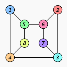
Figure 1: Cube graph representation.

Definition 1.3.

The edge that consists of the same elements is called loop.

Definition 1.4.

The subset of edges that consists of the same elements is called multiple edges (or multi-edge).

Example 1.2.

$(1,1)$ — loop,

$((1,2),(1,2),(1,2))$ — multiple edges.

NB! Now and further we will consider only so-called simple graphs — graphs without loops and multiple edges unless otherwise specified.

There is important difference between simple directed graph and simple undirected graph. Be aware about the case $((1,2),(2,1))$.

Definition 1.5.

Directed graph is called oriented graph if there are no two-side edges between any two vertices of the graph.

Definition 1.6.

Sub-graph is the part of the graph that is a graph.

NB! One can consider isolated vertices by adding the set of vertices to edges, but this or similar definition give rise many problems further, so we omit it.

Definition 1.7.

Maximum sub-graph on the current subset of graph vertices is the maximum by inclusion of edges sub-graph whose set of vertices is the current set.

Definition 1.8.

Two graphs are called isomorphic if one can re-number the vertices of one graph to obtain another.

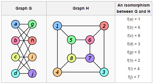
Figure 2: Example of isomorphism.

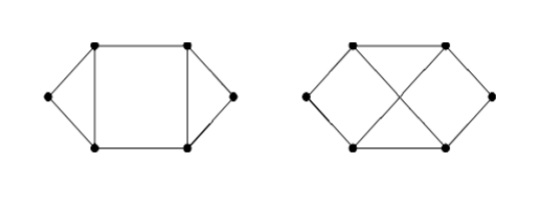
Figure 3: Example of non-isomorphic graphs.

Remark 1.1.

To prove that two graphs in figure 3 are non-isomorphic compare the structures of their sub-graphs.

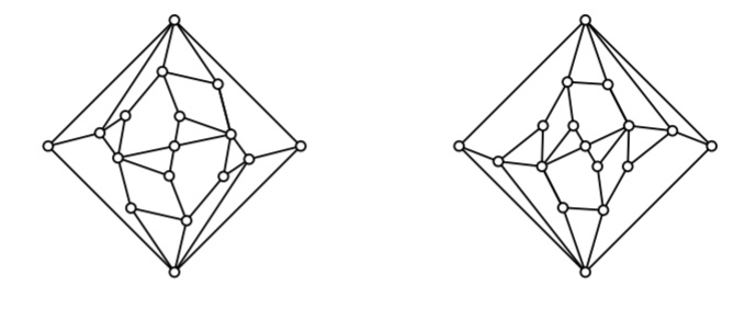
Figure 4: Are these graphs isomorphic or not?

It is simple to prove the graph isomorphism in special cases like in figure 3 but in general this proof is NP-hardness problem. Try to solve the problem in figure 4.

NB! Isomorphic graphs are also called the same graphs.

Definition 1.9.

Degree of vertex $\mathbf{v_{i}}\ (\deg{v_{i}})$ is the number of edges which are coming out from the vertex $v_{i}$.

In different books and articles definition of degree may vary: it can be defined by in-edges and also by whole edges (sum of in- and out-edges), but here the out-edges definition will be used.

Definition 1.10.

A vertex is called even (odd) if it has even (odd) degree.

Lemma 1.

(Handshaking lemma).

$$\sum_{v_{i}\in V}{\deg{v_{i}}}=2\|E\|.$$

[1em]0em

Proof.

Note that in $\sum_{v_{i}\in V}{\deg{v_{i}}}$ every edge occurs 2 times. ∎

Example 1.3.

Consider the bit representation of numbers
from 0 to $2^{n}-1$. Define the graph of n-dimensional cube by
following:

1. $V=\{\text{i for i from 0 to }2^{n}-1\}$,

2. $E=\{\text{(i,j) iff. i and j differ only in one bit}\}.$

How many edges has n-dimensional cube for any n?

[1em]0em

Proof.

The cases $n=1,2,3$ are well-known: it is segment,
square and cube with 1, 4 and 12 edges correspondingly.
For another cases let’s use Handshaking lemma:

$2\|E\|=\sum_{v_{i}\in V}{\deg{v_{i}}}=\|V\|\deg{v_{i}}=n\,2^{n}$.

Thus $\|E\|=n\,2^{n-1}$. ∎

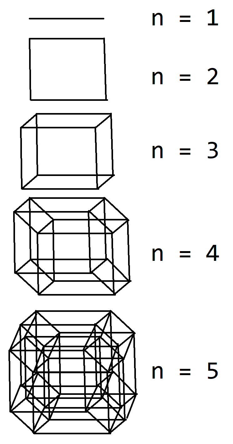
Figure 5: Graphs of hypercubes.

Definition 1.11.

Path is the sequence of edges in which ending and beginning vertices of consecutive edges are coincide.

Definition 1.12.

Graph is called weighted if each edge $e_{ij}$ corresponds to a number $w_{ij}\in\mathbb{R}$.

One can consider edges with zero weight but this correspondence may lead to many problems in following definitions and algorithms e.g. adjacency matrix, incidence matrix and so on.

2 Two matrices corresponded to a graph

2.1 Adjacency matrix

Definition 2.1.

Let’s define adjacency matrix A(G) for unweighted directed graph G by following:

$$A(G)=\{a_{ij}\}:=\begin{cases}1&\text{if there exists edge from vertex $v_{i}$ to vertex $v_{j}$}\\ 0&\text{otherwise}\end{cases}.$$

NB! For weighted directed graph adjacency matrix (or weight adjacency matrix) is defined equivalently, but instead of 1 will be weight $w_{ij}$ of corresponding edge.

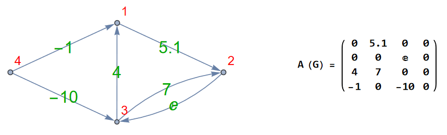
Figure 6: Example of a graph and its adjacency matrix.

Properties of adjacency matrix:

1. Adjacency matrix is symmetrical for undirected graph

2. Adjacency matrix diagonal elements equal to 0 (no loops)

3. Adjacency matrix always square matrix

4. For unweighted graph adjacency matrix consists of 0 and 1 and

   $$\deg{v_{i}}=\{\text{the sum of row $i$ elements}\}$$

5. “Adjacence” correspondence between weighted directed graphs and matrices with properties 2-3 is one-to-one if 0 weights are excluded

Theorem 1.

The number of paths from vertex $v_{i}$ to $v_{j}$ of length $k$ is equal to $(A(G)^{k})_{ij}$ for unweighted graph G.

[1em]0em

Proof.

Let’s consider the induction by k:

1. The number of paths from vertex $v_{i}$ to $v_{j}$ of the length 1 corresponds to existence of the edge $e_{ij}$.

   $$\{a_{rj}\}=\begin{cases}1&\text{if there is edge from vertex $v_{r}$ to $v_{j}$}\\ 0&\text{otherwise}\end{cases}.$$

2. Suppose the induction statement holds for any given case k, then

   $$(A^{k+1})_{ij}=(A^{k})_{ir}a_{rj}=\sum_{v_{r}\in V}{\{\text{Number of paths from vertex $v_{i}$ to $v_{r}$ with length $k$\}*}}$$

                 *{1 if there is edge from $$v_{r} v_{j}$$ to , 0 - overwise.} =

   = {Number of paths from vertex $$v_{i} v_{j} k+1$$ to of length }.

∎

2.2 Incidence matrix

Consider unweighted directed graph $G$ with some numeration of edges.

Definition 2.2.

Incidence matrix is defined for unweighted directed graph $G$ and its edges numeration by following:

$$B(G)=\{b_{ij}\}=\begin{cases}1&\text{if edge $j$ starts from vertex $v_{i}$}\\ -1&\text{if edge $j$ ends in vertex $v_{i}$}\\ 0&\text{otherwise}\end{cases}.$$

NB! For unweighted undirected graph incidence matrix is defined equivalently, but instead of -1 will be 1.

NB! To generalize incidence matrix definition for weighted graphs (or weighted incidence matrix) multiply each column by weight of corresponding edge.

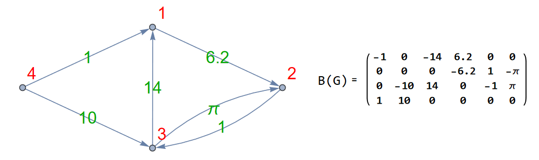
Figure 7: Example of graph and its incidence matrix.

Properties of incidence matrix:

1. In each column of incidence matrix there are only two non-zero elements

2. Incidence matrix is rectangular matrix with dimensions $\|V\|\times\|E\|$

3. The sum of elements in each incidence matrix column equals to 0 for directed graphs

4. For unweighted undirected graph incidence matrix consists of 0 and 1 and

   $$\deg{v_{i}}=\{\text{the sum of row $i$ elements}\}$$

5. “Incidence” correspondence between weighted directed graphs and matrices with properties 2-4 is one-to-one up to column permutations if non-positive weights are excluded

3 Connectivity and trees

Definition 3.1.

Graph is called connected iff. there exists path between any two vertices.

Definition 3.2.

Connected component of the graph is connected sub-graph that is not part of any larger connected sub-graph.

For directed graph there exist several connectivity definitions: weakly connectivity (if replacing of directed edges to undirected edges produces a connected undirected graph), semiconnectivity (if there exists one-side path between any two vertices) and strong connectivity (if there exists path between any two vertices from one to another and vise versa). For each of these connectivity one can define corresponded connected component, but we will consider properties and prove theorems only for undirected case here and in the next section.

Let’s consider some simplest necessary and sufficient conditions of connectivity.

Lemma 2 (Odd vertices lemma).

The number of odd vertices in each connected component of undirected graph is even.

[1em]0em

Proof.

Use Handshaking lemma for each connected component. ∎

Theorem 2.

(Connectivity necessary condition). Consider the undirected graph $G(n,k)$. If $k>C_{n-1}^{2}$, then graph G is connected.

[1em]0em

Proof.

Assume the contrary: there exist greater or equal than two connected components. Denote one component by $G_{1}$ and all the rest by $G_{2}$. Hence, $G=G_{1}\sqcup G_{2}$.
Consider two cases:

1. Let $\|V(G_{1})\|=n-1,\|V(G_{2})\|=1\implies\|E(G)\|=\|E(G_{1})\|\leq C_{n-1}^{2}$ — the maximum number of edges in undirected graph with $n-1$ vertices.
   The same for $\|V(G_{1})\|=1,\|V(G_{2})\|=n-1$.

2. Let $2\leq\|V(G_{1})\|=k\leq n-2\implies$

   $$\|E(G)\|=\|E(G_{1})\|+\|E(G_{2})\|\leq C_{k}^{2}+C_{n-k}^{2}=\frac{2k^{2}+n^{2}-2nk-n}{2}\vee C_{n-1}^{2}=\frac{n^{2}-n}{2}$$

   $$n-1+k^{2}-nk\vee 0$$

   $$(k-1)(k-n+1)\leq 0$$

   This gives a contradiction, since $\|E(G)\|>C_{n-1}^{2}$.

∎

Definition 3.3.

Cycle is a path consisted from distinct edges where the first and last vertices coincide.

Definition 3.4.

Simple path is a path where any edges and vertices are distinct except the first and the last vertices.

Definition 3.5.

Simple cycle is a simple path where the first and last vertices coincide.

Lemma 3.

The graph contains a cycle iff. it contains a simple cycle.

[1em]0em

Proof.

1. If the graph contains a simple cycle then it obviously contains a cycle.

2. Consider the graph that contains a cycle. Let’s construct the simple cycle: start from any vertex of the cycle and walk through the cycle and delete visited edges. Since the cycle is finite, a visited vertex will be reached after several steps. The cycle corresponded to this walk to the first visited vertex is a simple cycle.

∎

Definition 3.6.

Tree is undirected connected acyclic (without cycles) graph.

Another definition of tree holds from the lemma 3: tree is undirected connected graph without simple cycles.

Definition 3.7.

Polytree is an oriented graph whose underling undirected graph is a tree.

Definition 3.8.

Tree leaf is a vertex of degree 1.

Definition 3.9.

Tree root is any highlighted vertex of the graph.

NB! The root is any highlighted vertex of the graph, however the leafs, in general, are not highlighted as roots.

Definition 3.10.

Arborescence of a directed graph is the polytree that consist of all vertices of the graph that can be reached from the root.

Lemma 4 (Two leafs lemma).

Every tree contains two leafs.

[1em]0em

Proof.

The method is the same as in previous lemma. Let’s start walking from any vertex and deleting visited edges. Since the graph is finite a dead end will be reached after several steps. The end corresponds to first leaf. Starting this procedure again from the leaf will provide the second. ∎

Lemma 5 (Uniqueness path lemma).

There exists unique path between any two vertices of tree.

[1em]0em

Proof.

Hint: assume the contrary and find cycle. ∎

4 Spanning trees and algorithms

4.1 Spanning trees of unweighted graph

Definition 4.1.

Spanning tree of undirected graph is a tree that contains all vertices of the graph.

NB! The spanning trees exist only for undirected connected graphs. For not connected graph there is another definition — spanning forest.

Consider the base algorithms for constructing spanning trees:

1. Depth-first search (DFS) is the algorithm for searching elements in tree-structured data. Here we discuss it from constructing spanning trees point of view.

   Description:

   1. Start from the root. The root is assigned first number.

   2. Walks through non-assigned sub-graph and assign traversed vertices by consecutive numbers (from second). If it is dead end, return to the previous steps as long as you can continue.

   3. Go to step 1b.

   The assigned numbers form depth-first order.
   
   To construct spanning tree, you should save edges on the step 1b from previous assigned vertex to the new one that has to be assigned (see figure 8).

2. Breadth-first search (BFS) is also the algorithm for searching elements in tree-structured data. Here we discuss it from constructing spanning trees point of view.

   Description:

   1. Start from the root. The root is assigned first number.

   2. Consider the vertex as visited and walk through all edges from it to non-assigned vertices and assign them by consecutive numbers (from second).

   3. Select the next (up to assigning) not visited vertex and go to step 2b.

   The assigned numbers form breadth-first order.
   
   To construct spanning tree, you should save edges on the step 2b from selected vertex to new vertices which have to be assigned (see figure 8).

NB! It is easy to see, that the complexity of these algorithms equals to $\mathbf{O(\|V\|+\|E\|)}$.

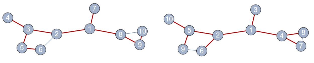
Figure 8: Depth-first search (left) and breadth-first search (right) algorithms, orders and corresponding spanning trees.

Depth-first search and breadth-first search algorithms produces different spanning trees in general. Spanning tree from depth-first search algorithm is called Trémaux tree, while from breadth-first search just breadth-first tree. Also there is freedom to choose a walking direction. Different directions produce different spanning trees as well.

For not connected graphs these algorithms also can be used. In this case they will construct spanning trees for the connected component of the root. By changing root between components one can construct spanning trees for each component so-called spanning forest.

NB! These algorithms can by applied for checking connectivity condition of the graph.

Theorem 3 (Necessary and sufficient tree condition 1).

A graph with $n$ vertices is tree iff. it is connected and consists of $n-1$ edges.

[1em]0em

Proof.

1. Necessarity. The induction by number of vertices:

   1. For graph (1, 0) holds.

   2. Let for every tree with $n$ vertices the condition holds. Consider tree $T$ with $n+1$ vertices. This tree contains two leafs by lemma 4. By deleting one of these leafs the graph will become a tree $T^{\prime}$ with $n$ vertices and edges decreased by 1. The tree $T^{\prime}$ consists of $n-1$ edges by inductive hypothesis, therefore $T$ consists of $n$ edges.

2. Sufficiency. Construct the spanning tree of the graph by one of algorithms above. The spanning tree consists of $n-1$ edges.

∎

Theorem 4 (Necessary and sufficient tree condition 2).

A graph with $n$ vertices is tree iff. it is acyclic and consists of $n-1$ edges.

[1em]0em

Proof.

1. Necessarity. Holds from theorem 3.

2. Sufficiency. Let the number of connected components be $k$. Construct the spanning tree for every component. Each component is tree, therefore the whole number of edges equals $n-k$ ($-1$ for every component)$\implies k=1$ and the graph is connected.

∎

NB! By these theorems, one can rewrite the complexity of depth-first search and breadth-first search algorithms for connected graphs as $\mathbf{O(\|V\|+\|E\|)}=\mathbf{O(\|E\|)}$.

4.2 Minimum spanning trees of weighted graph

For weighted graph there exists another kind of spanning tree:

Definition 4.2.

Minimum spanning tree is the spanning tree with minimum total edge weight.

Consider two basic algorithms for constructing minimum spanning tree. These algorithms belong to large area called greedy algorithms (in which making the locally optimal choice at each stage leads to globally optimal solution).

1. Prim’s algorithm.
   Description:

   1. Start from arbitrarily vertex. This vertex is the tree $T$.

   2. Let the $K(T)$ — edges $\not\in T$ adjacent to any vertex $\in T$. Add to the tree $T$ new edge with minimal weight in $K(T)$ that is not produce the cycle in $T$ and vertices incident to the edge.

   3. Do 1b step $\|V\|-1$ times.

2. Kruskal’s algorithm.
   Description:

   1. Start from arbitrarily vertex. This vertex is the tree $T$.

   2. Let the $K(T)$ — all edges $\not\in T$. Add to the tree $T$ new edge with minimal weight in $K(T)$ that is not produce the cycle in $T$ and vertices incident to the edge.

   3. Do 2b step $\|V\|-1$ times.

NB! The Prim’s and Kruskal’s algorithms complexity is $\mathbf{O(\|E\|\,log(\|V\|))}$.

Minimum spanning trees from Prim’s and Kruskal’s algorithms depend of the first selected vertex and also of the edge from equal weights set.

Remark 4.1.

The proof of correctness Prim’s and Kruskal’s algorithms holds from theorem 3 and theorem 4 correspondingly or from greedy property.

Each of these algorithms has its pros and cons: Prim’s algorithm produces connected graph for each step but binary heap and adjacency list should be used to reach $O(\|E\|\,log(\|V\|))$ complexity. Kruskal’s algorithm reach this complexity by using simpler structures.

5 Laplacian matrix and Kirchhoff’s theorem

As in previous two sections let’s consider undirected unweighted graph $G$.

Definition 5.1.

Laplacian matrix is defined for undirected unweighted graph $G$ by following:

$$L(G)=\{l_{ij}\}=\begin{cases}\deg{v_{i}}&\text{if $i=j$}\\ -1&\text{if there exists edge from vertex $v_{i}$ to vertex $v_{j}$}\\ 0&\text{otherwise}\end{cases}.$$

Or equivalently:

$$L(G)=\mathrm{Diag}\{\deg{v_{i}}\,|\,v_{i}\in V\}-A(G).$$

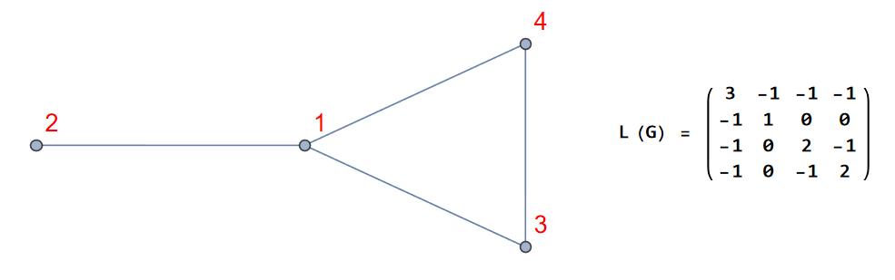
Figure 9: Example of a graph and its laplacian matrix.

Properties of laplacian matrix:

1. Laplacian matrix non-diagonal part consists of 0 and -1 elements

2. Laplacian matrix is symmetrical matrix

3. Laplacian matrix is square matrix

4. The sum of elements in each laplacian matrix column (and row) equals to 0

5. Laplacian matrix is degenerate matrix

6. “Laplacian” correspondence between undirected unweighted graphs and matrices with properties 1-4 is one-to-one

Lemma 6 (Laplacian matrix algebraic complements lemma).

Algebraic complements of all Laplacian matrix elements are equal.

[1em]0em

Proof.

Denote the number of vertices of a graph $G$ by $n$ and the algebraic complement to the element $l_{ij}$ of Laplacian matrix by $L_{ij}$.

1. Let $\text{rk(L(G))}<n-1\implies L_{ij}=0,\text{for any }i,j$.

2. $\text{rk(L(G))}=n-1$. Let’s denote the column of $n$ 1’s by $m$, the matrix of complements $\{L_{ij}\}$ by $M$ and the columns of $M^{T}$ by $\{m_{j}\}$. Hence, $Lm=0$ due to Laplacian matrix property 4 and

   $$LM^{T}=\det(L)I=0\implies Lm_{j}=0,\text{for }j=1...n.$$

   Consider the linear equation $Lx=0$. Since the $\text{rk(L(G))}=n-1$, the solutions of the equation form a one-dimensional linear space. The vector $m$ is a solution of the equation, hence all other solutions ($m_{1},m_{2},...,m_{n}$) are proportional to $m$ and therefore consist of equal elements. The symmetry property of the Laplacian matrix implies the assertion of the theorem.

∎

Lemma 7 (Laplacian and incidence matrix lemma).

$L=B\,B^{T}$, where $B$ is the incidence matrix for any orientation of the graph and numeration of the edges.

[1em]0em

Proof.

Consider any orientation and numeration of the edges of undirected graph and let $B$ be its corresponding incidence matrix. Denote the row $i$ of the matrix $B$ as $b_{i}$ and by $n$ the number of vertices of the graph.

$$B\,B^{T}=\{m_{ij}\}=\{b_{i}\cdot b_{j}\}.$$

1. For $i=j$, $m_{ii}=b_{i}^{2}=\{\text{the number of non-zero elements in }b_{i}\}=$
   $=\{\text{the sum of elements in $i$ row in the incidence matrix for undirected graph}\}=\deg{v_{i}}$, due to incidence matrix property 4.

2. For $i\neq j$,

   $$b_{ik}\ b_{jk}=\begin{cases}-1&\text{if $v_{i}$ adjacent to $v_{j}$ by the edge $k$}\\ 0&\text{otherwise}\end{cases}.$$

   Since the graph has no loops,

   $$m_{ij}=b_{i}\cdot b_{j}=\sum_{k=1}^{n}{b_{ik}b_{jk}}=l_{ij}.$$

∎

Lemma 8 (Graph $(n,n-1)$ lemma).

Let $B(G)$ — the incidence matrix for some orientation and numeration edges of the graph $G(n,n-1)$ and $D(B)$ be maximum principal minor of the matrix $B$. It follows, that

1. $D(B)=\pm 1$, if $G$ is connected (tree),

2. $D(B)=0$, if $G$ is not connected (not tree).

[1em]0em

Proof.

1. Let the graph $G$ be connected. The graph $G$ is tree by the theorem 3 and therefore it has at least two leafs by lemma 4.

   For the graph $G(n,n-1)$ the matrix $B(G)$ is also $n\times(n-1)$ matrix, hence the maximum principal minor is the determinant of matrix $B(G)$ without some row. Suppose that this row corresponds to last vertex $v_{n}$ without loss of generality (if it is not, re-number vertices).

   1. Consider the leaf $\neq v_{n}$ and the edge adjacent to the leaf. Re-number vertices and edges such that this leaf becomes first vertex $v_{1}$ and its adjacent edge becomes the first edge $e_{1}$. This re-numbering procedure corresponds to row and column permutations in the matrix $B(G)$ and in the determinant $D(B)$, therefore $D(B)$ is not changing. By this re-numbering the first row of the matrix $B(G)$ becomes equal to $(\pm 1,0,0,...,0)$.

   2. Consider the maximum sub-graph on $V(G)\setminus\{v_{1}\}$ vertices and do the same procedure as in 1a for this sub-graph. Thus, the corresponding vertex and the edge becomes the second vertex and edge and the second row of the matrix $B(G)$ will looks like $(*,\pm 1,0,0,...,0)$, where “*” means some number. Let’s continue this procedure.

   3. In the end, the matrix $B(G)$ will looks like $\begin{pmatrix}\pm 1&0&0&...&0\\ *&\pm 1&0&...&0\\ *&*&\pm 1&...&0\\ &&...&&\\ *&*&*&...&\pm 1\\ *&*&*&...&*\end{pmatrix}$.
      And $D(B)$ will be the determinant of the upper part of the matrix. Therefore, $D(B)=\pm 1$.

2. Suppose the graph $G$ is not connected. Denote by $G_{1}$ the connected component without vertex $v_{n}$ and $G_{2}$ all the rest.

   Consider the sub-matrix $K\subset B(G)$ corresponding to vertices of $G_{1}$. The incidence matrix $B(G_{1})$ is the sub-matrix of the matrix $K$. The sum in each column of the matrix $K$ equals to 0: if edge belongs to $G_{1}$ then the sum equals to 0 by property 3 of incidence matrix $B(G_{1})$ and if edge belongs to $G_{2}$ then all elements in corresponding column equals 0. Hence, the sum of rows of the matrix $K$ equals 0. Since $K$ is the part of the matrix corresponding to $D(B)$, the determinant $D(B)=0$.

∎

Theorem 5 (Kirchhoff matrix tree theorem).

The number of trees in undirected unweighted connected graph $G$ equals to the algebraic complement of any Laplacian matrix element.

[1em]0em

Proof.

From Lemma 7: $L(G)=B\,B^{T}$. Denote the number of vertices of graph G by $n$. Algebraic complements of all Laplacian matrix elements are equal by the lemma 6. Consider the algebraic complement $L_{nn}$ of the last right element $l_{nn}$. Let’s denote $\hat{B}$ the matrix $B(G)$ without last row. Therefore, $L_{nn}=\hat{B}\,\hat{B}^{T}$.

Since the graph is connected the number of edges is $\geq n-1\implies$ the principal minor $D(\hat{B})$ of the matrix $\hat{B}$ has $(n-1)\times(n-1)$ dimensions. Let $T(B)$ be the sub-matrix of $B$ consisted of the columns corresponding to $D(\hat{B})$ (see Figure 10). The sub-matrix $T(B)$ is obtained by adding to $D(\hat{B})$ last row and hence has $n\times(n-1)$ dimensions. Therefore, the sub-matrix $T(B)$ corresponds to a sub-graph $\hat{G}(n,n-1)\subset G$. Moreover, this matrix equals to incidence matrix of the sub-graph $B(\hat{G})$ (to proof this part more accurately, one should either consider the definition of sub-graph with isolated vertices or proof this part in terms of sub-matrices). By the lemma 8:

$$D(T(B))=D(B(\hat{G}))=\begin{cases}\pm 1&\text{if $\hat{G}$ is tree}\\ 0&\text{if it is not}\end{cases},$$

and it is also equal to $D(\hat{B})$.

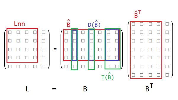
Figure 10: Designations in the Kirchhoff matrix theorem proof.

The last step is to use a formula from algebra:

Lemma (Binet-Cauchy formula).

Consider the matrix equation:

$$\begin{matrix}P&\times&Q&=&C\\ s\times t&&t\times s&&s\times s\end{matrix}$$

for two rectangular matrices $P$ and $Q$ of $s\times t$ and $t\times s$ dimensions and square $s\times s$ matrix $C$ for any $s,t\in\mathbb{N}$.

Let the columns of matrix $P$ be called “corresponded” to rows of matrix $Q$ iff. they are consist of the same sets of indexes. Denote the minors consisted of the corresponding columns and rows by $P_{i_{1}i_{2}...i_{s}}$ and $Q_{i_{1}i_{2}...i_{s}}$, for indexes $i_{1},i_{2},...,i_{s}\in\{1...t\}$ with repetitions.

It follows, that

$$\det{C}=\sum_{i_{1},i_{2},...,i_{s}=1}^{t}{P_{i_{1}i_{2}...i_{s}}\,Q_{i_{1}i_{2}...i_{s}}}$$

[1em]0em

Proof.

The complete proof won’t be provided here, just the main ideas:

1. For case $s=t$, it is well-known determinant of two matrices product: $\det{(P\,Q)}=\det{P}\det{Q}$.

2. For case $s>t$, the determinants $P_{i_{1}i_{2}...i_{s}}$ and $Q_{i_{1}i_{2}...i_{s}}=0$ for any $i_{1}i_{2}...i_{s}$ because of repetitions and $\text{rk(P\,Q)}\leq\text{rk(P)}\leq t\implies\det{C}=0$.

3. For case $s<t$, it follows from two algebraic facts:

   1. The coefficient of $z^{t-k}$ in the polynomial $\det{(zI_{t}+C)}$ is the sum of the $k\times k$ principal minors of $C$ for any $k\in\{1..t\}$, where $I_{t}$ is the identity matrix of $t\times t$ dimensions.

   2. If $s\leq t$, then $\det{(zI_{t}+Q\,P)}=z^{t-s}\det{(zI_{s}+P\,Q)}$, for matrices $P$ and $Q$ from the statement.

∎

Using the Binet-Cauchy formula for matrices $L_{nn}=\hat{B}\,\hat{B}^{T}$:

$$L_{nn}=\sum_{i_{1},i_{2},...,i_{n-1}}{\hat{B}_{i_{1}i_{2}...i_{n-1}}\,\hat{B}_{i_{1}i_{2}...i_{n-1}}^{T}}=\sum_{i_{1},i_{2},...,i_{n-1}}{D_{i_{1}i_{2}...i_{n-1}}^{2}(\hat{B})}=\sum_{\hat{G}(n,n-1)\subset G}{D^{2}(B(\hat{G}))},$$

and by the lemma 8 it equals to the number of spanning trees of $G$.

∎

Definition 5.2.

The complete graph $K_{n}$ is the graph where any two vertices are connected with an edge.

Theorem 6 (Cayley’s formula).

The number of spanning trees of the complete graph $K_{n}$ equals to $n^{n-2}$.

[1em]0em

Proof.

The Laplacian matrix for the complete graph is

$$L(G)=\begin{pmatrix}n-1&-1&-1&...&-1\\ -1&n-1&-1&...&-1\\ &&&...&\\ -1&-1&...&-1&n-1\end{pmatrix},$$

of dimensions $n\times n$.

The algebraic complement to the last element $l_{nn}$ is the determinant of the matrix of dimensions $(n-1)\times(n-1)$. Let’s find this algebraic complement.

$$L_{nn}=\det\begin{pmatrix}n-1&-1&-1&...&-1\\ -1&n-1&-1&...&-1\\ &&&...&\\ -1&-1&...&-1&n-1\end{pmatrix}\stackrel{{\scriptstyle\text{adding all rows to first}}}{{=}}\det\begin{pmatrix}1&1&1&...&1\\ -1&n-1&-1&...&-1\\ &&&...&\\ -1&-1&...&-1&n-1\end{pmatrix}=$$

$$\stackrel{{\scriptstyle\text{adding row column to others}}}{{=}}\begin{pmatrix}1&1&1&...&1\\ 0&n&0&...&0\\ &&&...&\\ 0&0&...&0&n\end{pmatrix}=n^{n-2}.$$

∎

6 Bipartite graph

Definition 6.1.

Connected undirected graph is called bipartite iff. one can divide the vertices into two groups such that any two vertices from one group are not adjacent.

Consider the bipartite property testing algorithm:

1. Choose any vertex.

2. Start depth-first or breadth-first algorithms and divide vertices to 0 or 1 groups by putting to them corresponded marks:

   1. For depth-first: sequentially alternate marks for depth-first walk.

   2. For breadth-first: put the same marks if the vertices are on the same breadth and change marks otherwise.

3. If any two vertices from one group are not adjacent, the graph is bipartite and not bipartite otherwise.

NB! The complexity of this algorithm is the same as for depth-first and breadth-first algorithms for connected graphs and equals to $\mathbf{O(\|E\|)}$.

Example 6.1.

Consider the result of the testing algorithm:

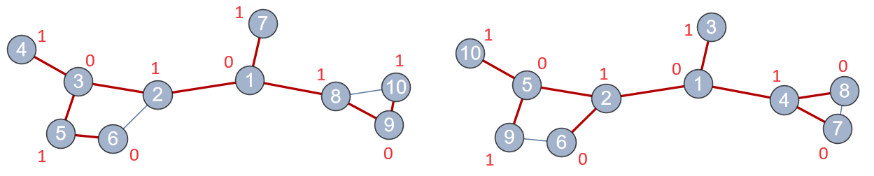
Figure 11: Group division (red marks) by depth-first algorithm (left) and breadth-first algorithm (right).

This graph is not bipartite because after the algorithm there are adjacent vertices from the same group.

Theorem 7 (Necessary and sufficient bipartite condition).

Connected undirected graph is bipartite iff. it doesn’t contain odd length cycles.

[1em]0em

Proof.

1. Necessarity. Assume the contrary: the graph contains odd length cycle. Let’s start to divide vertices from this cycle to two groups by the rule: two vertices from one group should not be adjacent. By this rule vertices will sequentially alternate to each other. Since the length of cycle is odd, the first and the last vertices will be from the same group. This gives a contradiction with bipartite condition.

2. Sufficiency. Consider bipartite property testing algorithm with spanning tree $T$ construction. It is easy to see that any tree is a bipartite graph. Let’s start to add remaining edges. Denote first edge by $(v,w)$.

   Assume that vertices $v$ and $w$ corresponds to the same group by the testing algorithm. By the lemma 5 there exists unique path from $v$ to $w$ in $T$. Since the marks alternate to each other along this path by the algorithm, this path with the edge $(v,w)$ form an odd length cycle. This gives a contradiction. Hence, all remaining edges connect vertices from different groups.

∎

Definition 6.2.

Bipartite graph is called complete bipartite graph $K_{n,m}$ iff. any two vertices from different groups are connected with an edge.

Theorem 8 (Cayley’s formula for bipartite graphs).

The number of spanning trees of the complete bipartite graph $K_{n,m}$ equals to $n^{m-1}m^{n-1}$.

[1em]0em

Proof.

The Laplacian matrix for the complete bipartite graph consists of 4 blocks:

$$L(G)=\begin{pmatrix}m&0&0&...&0&-1&-1&...&-1&-1\\ 0&m&0&...&0&-1&-1&...&-1&-1\\ &&&...&&&&...&&\\ 0&0&...&0&m&-1&-1&...&-1&-1\\ -1&-1&...&-1&-1&n&0&0&...&0\\ -1&-1&...&-1&-1&0&n&0&...&0\\ &&...&&&&&&...&\\ -1&-1&...&-1&-1&0&0&...&0&n\\ \end{pmatrix}.$$

The first upper-left corner with $m$’s has $n\times n$ dimensions and the last lower-right corner with $n$’s has $m\times m$ dimensions.

The algebraic complement to the last element $l_{nn}$ is the determinant of the matrix of dimensions $(n+m-1)\times(n+m-1)$. Let’s find this algebraic complement.

$$L_{nn}=\det\begin{pmatrix}m&0&0&...&0&-1&-1&...&-1&-1\\ 0&m&0&...&0&-1&-1&...&-1&-1\\ &&&...&&&&...&&\\ 0&0&...&0&m&-1&-1&...&-1&-1\\ -1&-1&...&-1&-1&n&0&0&...&0\\ -1&-1&...&-1&-1&0&n&0&...&0\\ &&...&&&&&&...&\\ -1&-1&...&-1&-1&0&0&...&0&n\\ \end{pmatrix}\stackrel{{\scriptstyle\text{adding all rows to first}}}{{=}}$$

$$=\det\begin{pmatrix}1&1&1&...&1&0&0&...&0&0\\ 0&m&0&...&0&-1&-1&...&-1&-1\\ &&&...&&&&...&&\\ 0&0&...&0&m&-1&-1&...&-1&-1\\ -1&-1&...&-1&-1&n&0&0&...&0\\ -1&-1&...&-1&-1&0&n&0&...&0\\ &&...&&&&&&...&\\ -1&-1&...&-1&-1&0&0&...&0&n\\ \end{pmatrix}\stackrel{{\scriptstyle\text{adding first row to the last $m-1$'s}}}{{=}}$$

$$=\det\begin{pmatrix}1&1&1&...&1&0&0&...&0&0\\ 0&m&0&...&0&-1&-1&...&-1&-1\\ &&&...&&&&...&&\\ 0&0&...&0&m&-1&-1&...&-1&-1\\ 0&0&...&0&0&n&0&0&...&0\\ 0&0&...&0&0&0&n&0&...&0\\ &&...&&&&&&...&\\ 0&0&...&0&0&0&0&...&0&n\\ \end{pmatrix}=m^{n-1}n^{m-1}.$$

∎

7 Shortest path problems

In this section the basic algorithms of searching shortest path between vertices in weighted directed or undirected graphs will be observed.

Definition 7.1.

The cycle in weighted graph is called negative cycle if the sum of weights along the cycle is negative.

If the path between two vertices intersects negative cycle, the shortest path between them is not exist. Therefore, for shortest path algorithms we consider only graphs without negative cycles unless otherwise specified.

These algorithms are very similar for both directed and undirected cases, so let’s give combined definition:

Definition 7.2.

The spanning tree of weighted (directed)undirected graph $G$ is called shortest path (arborescence)tree if the path from the root to any other vertex along the (poly)tree is the shortest path in $G$.

Consider basic algorithms:

1. Dijkstra’s algorithm.

   This algorithm finds the shortest path (arborescence)tree with selected vertex as a root for (directed)undirected graph with positive weights.

   Description:

   1. Initialization: mark all vertices unvisited, initialize two arrays: $d[v]$ — array with minimal distances and $p[v]$ — array with predecessors for shortest paths from the root to vertices $v$ and assign $d[v]$ by zero for the selected vertex and infinities for all others.

   2. Find the unvisited vertex $v$ with the smallest value in $d$. For each its unvisided neighbour $w$ if the sum of $d[v]$ plus weight of the edge $(v,w)$ is less than value $d[w]$, change $d[w]$ to the sum and change the predecessor $p[w]$ for $v$. After checking all unvisited neighbours mark $v$ visited.

   3. If there exist unvisited vertices in the graph go to 1b.

   Edges (predecessors and corresponded vertices) form shortest path tree (see figure 12).
   

   NB! The complexity of Dijkstra’s algorithm equals to $\mathbf{O(\|E\|+\|V\|^{2})=O(\|V\|^{2})}$ in the simplest realization. Using binary search tree or binary heap it equals to $\mathbf{O((\|E\|+\|V\|)\,log\,\|V\|)}$.

   

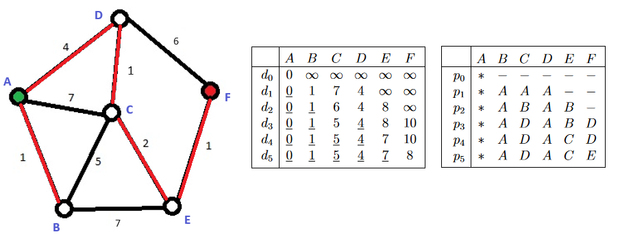
   Figure 12: Shortest path tree (left, red) and sequential steps of Dijkstra’s algorithm (right). The root vertex of the shortest path tree is denoted by “*”. Underlined numbers corresponded to visited vertices.

2. Bellman–Ford algorithm.

   This algorithm is similar to Dijkstra’s algorithm. It finds the shortest path (arborescence)tree with selected vertex as a root for any (directed)undirected graphs.

   Description:

   1. Initialize two arrays: $d[v]$ — array with minimal distances and $p[v]$ — array with predecessors for shortest paths from the root to vertices $v$ and assign $d[v]$ by zero for the selected vertex and infinities for all others.

   2. For each edge $(v,w)$ if the sum of $d[v]$ plus weight of the edge $(v,w)$ is less than value $d[w]$, change $d[w]$ to the sum and change the predecessor $p[w]$ for $v$.

   3. Do case 2b $\|V\|-1$ times.

   Edges (predecessors and corresponded vertices) form shortest path tree similar to Dijkstra’s algorithm (see figure 13).
   

   NB! The complexity of Bellman–Ford algorithm equals to $\mathbf{O(\|V\|\,\|E\|)}$.

   

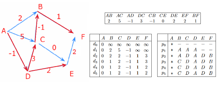
   Figure 13: Shortest path arborescence (left, red), the edge set of the graph (right-top) and sequential steps of Bellman–Ford algorithm (right-bottom). The root vertex of the shortest path arborescence is denoted by “*”.

   NB! Dijkstra’s and Bellman–Ford algorithms are also used for searching shortest path between two selected vertices for directed and undirected weighted graphs (walk along predecessors in reverse order to find the shortest path). Also, Dijkstra’s algorithm can be stopped earlier when the final vertex is visited and Bellman–Ford algorithm when the minimal distances array is not changed.
   

   Bellman–Ford algorithm also finds negative cycle in a graph. If the graph contains negative cycle, the shortest path between any two vertices of the cycle doesn’t exist and if one runs the algorithm one more time ($\|V\|$ times in total) the minimal distances array will change. Let’s consider this algorithm (see figure 14 for example):

   1. Do case 2b one more time.

   2. Find the vertex $v$, where $d[v]$ was changed.

   3. The negative cycle is obtained by saving vertices from this vertex $v$ along precursors array at previous $\|V\|$-1 step (in reverse order).

   

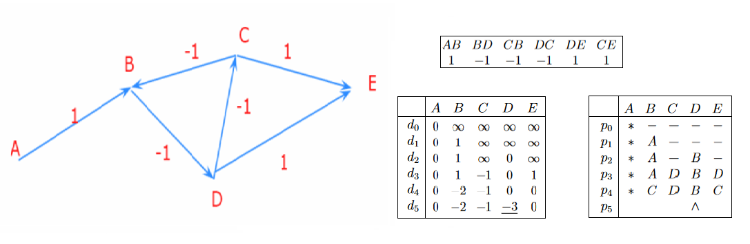
   Figure 14: Sequential steps of Bellman–Ford algorithm (right) for the graph (left). The starting vertex is denoted by “*”. Column (vertex) $D$ with underlined number corresponded to value that have changed on the additional $\|V\|$ step. The negative cycle $DCBD$ is constructed by walking along precursors set (in reverse order) from this vertex.

3. Floyd–Warshall algorithm.

   This algorithm finds the shortest path matrix $d[v][w]$ (shortest path between any two vertices) for the graph.

   Description:

   1. Initialize shortest path matrix $d[v][w]$: for every edge $(v,w)$ the element $d[v][w]$ is equal to weight of $(v,w)$ and $\infty$ otherwise.

   2. For each vertex $w$ check for each pair of vertices $v,u$ if the sum of $d[v][w]$ and $d[w][u]$ is less than $d[v][u]$. If it is then change $d[v][u]$ for this sum.

   NB! The complexity of Floyd–Warshall algorithm equals to $\mathbf{O(\|V\|^{3})}$.

4. Johnson’s algorithm.

   This algorithm finds the shortest path matrix for a graph by using Bellman–Ford shortest path tree and Dijkstra’s algorithm for weighted undirected connected graph and for directed graph if there exist paths from the root to any other vertex (spanning arborescence, see figure 15 for example).

   Description:

   1. Use Bellman–Ford algorithm, calculate minimal distances array $d[v]$ and check if the graph contains negative cycle.

   2. If the graph doesn’t contain negative cycle, correct all weights using Bellman–Ford’s values: change the weight of each edge $(v,w)$ to the sum of the weight and $d[v]-d[w]$.

   3. For each vertex use Dijkstra’s algorithm and calculate shortest path matrix.

   4. Correct shortest path matrix by reverse transformation: change each $d[v][w]$ to the difference between $d[v][w]$ and $d[v]-d[w]$.

   NB! The complexity of Johnson’s algorithm equals to $\mathbf{O(\|V\|\,\|E\|+(\|E\|+\|V\|)\|V\|\,log\|V\|)}=\mathbf{O((\|E\|+\|V\|)\|V\|\,log\|V\|)}$.

   After changing the weights of the graph by step 4b all weights become non-negative with zero-weights along Bellman–Ford’s arborescence. Using Dijkstra’s algorithm for each vertex it gives zero shortest path along the arborescence.

   

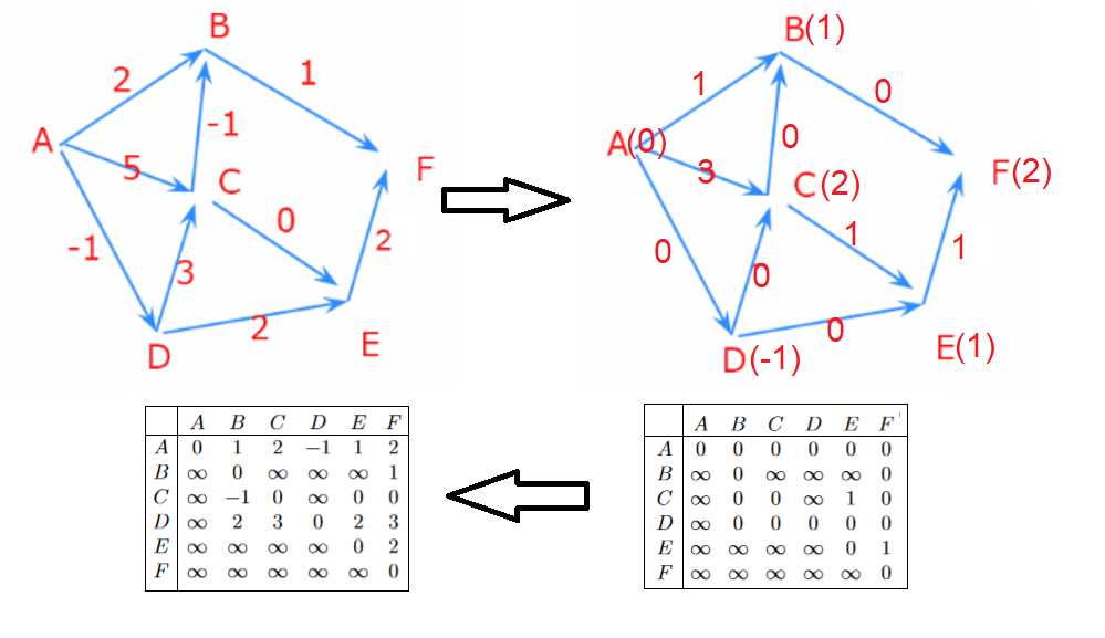
   Figure 15: First two steps of Johnson’s algorithm (top). Minimal distances lengths $d[v]$ for the first step are written near vertices in brackets. Weights of edges have been changed by second step. Shortest path matrix for graph with new weights by using Dijkstra’s algorithm (left-bottom). Result shortest path matrix (right-bottom).

8 Planar graph and polyhedrons

8.1 Planar graph

Definition 8.1.

A graph is called planar iff. there exists representation of the graph without intersections of edges.

Example 8.1.

1. Every tree is planar.

2. $K_{2},K_{3},K_{4}$ are planar.

3. $K_{5}$ is not planar.

4. $K_{1,2},K_{1,3},K_{2,2},K_{2,3}$ are planar.

5. $K_{3,3}$ is not planar.

[1em]0em

Proof.

1. It is easy to see that tree is planar (use Depth-first or breadth-first orders to prove it).

2. Just try to draw these graphs on plane without intersections.

3. To proof that $K_{5}$ is not planar let’s use classical theorem:

   Theorem (Jordan curve).

   Any simple closed curve $C$ divides the plane for two disjoint open subsets and any curve starting from point of the first subset and ending in the point of the second subset intersect $C$.

   These subsets are denoted by $int(C)$ — inner subset and $out(C)$ — outer subset.

   Consider the contrary. The cycle $C=v_{1}v_{2}v_{3}v_{1}$ is closed curve thus it divides the plane by two parts. Let’s suppose without loss of generality that $v_{4}\in int(C)$. Consider three cycles $C_{1}=v_{2}v_{3}v_{4}v_{2},C_{2}=v_{3}v_{4}v_{1}v_{3},C_{3}=v_{1}v_{2}v_{4}v_{1}$. Since $v_{i}\in out(C_{i})$ the assumption that $v_{5}\in int(C_{i})$ gives contradiction (the edge $(v_{5},v_{i})$ should intersect $C_{i}$ by Jordan curve theorem) therefore $v_{5}\in out(C_{i})$ for $i=1,2,3$. Hence, $v_{5}\in out(C)=\bigcap\limits^{3}_{i=1}out(C_{i})$ and it gives contradiction because $v_{4}\in int(C)$.

4. $K_{1,2},K_{1,3}$ are trees. For $K_{2,2},K_{2,3}$ just draw this graph on plane without intersections.

5. Use the same procedure like in 3.

∎

Definition 8.2.

Inner face of the planar graph is the inner $int(C)$ part of the plane bounded by a simple cycle $C$ of graph.

Notations: The set of all faces (inner and outer) is denoted by $F$.

Definition 8.3.

Outer face of the planar graph is the common outer part $out(G)$ for all simple cycles $C_{i}$ of graph $G:out(G)=\bigcap\limits_{i}out(C_{i})$.

NB! Any tree has only one outer face and no inner faces.

Theorem 9 (Euler).

For any planar connected graph the formula holds:

$$\|V\|-\|E\|+\|F\|=2.$$

[1em]0em

Proof.

Induction by number of faces $k=\|F\|$:

1. If graph contains only one face ($k=1$), this face should be outer face. If there are no inner faces then there are no cycles in the graph and therefore graph is tree. For tree $\|V\|=n,\|E\|=n-1$ and the condition holds.

2. Let for any planar connected graph with $k$ faces condition holds. Consider a planar connected graph with $k+1$ faces. Since the graph is planar there exists an edge (without intersections with any other edges) that separates the outer face and some inner face. If one delete this edge the number of faces will decrease at 1 and hence the formula will be satisfied. Therefore the condition holds for the initial graph also.

∎

Corollary 1.

Let $c$ be the number of connected components of a planar graph. Then the formula holds:

$$\|V\|-\|E\|+\|F\|=1+c.$$

[1em]0em

Proof.

Hint: for each connected component $H:\|V(H)\|-\|E(H)\|+\|F(H)\|=\text{outer face}+1$. ∎

Corollary 2.

For a connected planar graph $\|E\|\leq 3\|V\|-6$.

[1em]0em

Proof.

Consider the sub-graph of the graph $G$ that consist of union of all simple cycles of the graph. For this sub-graph: every simple cycle corresponded to some face and consists of $\leq 3$ edges and every edge belongs to a boundary of two different faces. Hence, for the graph $G:3\|F\|\leq 2\|E\|$. By the Euler’s theorem:

$$3\|F\|=6-3\|V\|+3\|E\|\leq 2\|E\|\implies\|E\|\leq 3\|V\|-6.$$

∎

Corollary 3.

Every connected planar graph has a vertex of degree at most five.

[1em]0em

Proof.

Assume the contrary: all vertices have degrees greater or equal than six. By Handshaking lemma $6\|V\|-12\geq 2\|E\|=\sum_{v_{i}\in V}{\deg{v_{i}}}\geq 6\|V\|$ holds contradiction. ∎

Let’s consider some operations of a planar graphs which preserve the planarity:

Lemma 9.

Every sub-graph of a planar graph is planar.

[1em]0em

Proof.

Holds from the definition. ∎

Definition 8.4.

Subdivision of an edge is an operation when the edge is replaced by a path of the length two: the internal vertex is added to the graph.

Lemma 10.

Every subdivision of the non-planar graph is non-planar.

[1em]0em

Proof.

Just consider the inverse operation. ∎

By these two lemma’s we can easy prove the necessary condition of the most important theorem about planar graphs:

Theorem (Pontryagin-Kuratowski).

A connected graph is planar iff. it doesn’t contain subdivisions of complete graphs $K_{5}$ and $K_{3,3}$.

We will provide the full proof of this theorem in section 12.

8.2 Polyhedrons

Definition 8.5.

Polyhedron is a set of polygons such that

1. Each side of a polygon should be the side of one another polygon,

2. The intersection of any two polygons can be just either edge of vertex,

3. There exists path through polygons between any two polygons.

Let’s introduce another theorem like Jordan curve theorem for hyper-surfaces in $\mathbb{R}^{n}$:

Theorem (Jordan-Brouwer).

Any connected compact simple hypersurface $S^{n-1}$ divides $\mathbb{R}^{n}$ for two disjoint open subsets and any curve starting from point of the first subset and ending in the point of the second subset intersect $S^{n-1}$.

We can consider each polyhedron $P$ like 2-dimensional surface in $\mathbb{R}^{3}$ and thus it divides the 3-dimensional space by two disjoint parts inner $int(P)$ and outer $out(P)$. The boundary of polyhedron is denoted by $\partial(P)$.

Definition 8.6.

Polyhedron is said to be convex iff. the edge from any point of polyhedron to any inner point doesn’t intersect the polyhedron.

This definition can be reformulate as any point of polyhedron is visible from any inner point.

Theorem 10 (Euler for convex polyhedrons).

For convex polyhedrons the following holds:

$$\|V\|-\|E\|+\|F\|=2,$$

where $V,E$ and $F$ are vertices, edges and faces of polyhedron respectively.

[1em]0em

Proof.

By the convex definition of the polyhedron there exists the bijection from polyhedron to the sphere around this polyhedron with the center in inner point. By this bijection the graph of polyhedron $G(P)$ is mapped to the graph on the sphere $G^{\prime}$ with the same number of vertices, edges and faces. Consider the stereographic projection from the sphere with the center inside some face $F_{i}$ of graph $G^{\prime}$ to the 2-dimensional plane. This graph $G^{\prime}$ maps bijectively (because of stereographic projection property, see figure 16) to the graph on the plane $G^{\prime\prime}$ such that inner faces of $G^{\prime}$ except $F_{i}$ maps to inner faces of $G^{\prime\prime}$ and $F_{i}$ maps to the outer face of $G^{\prime\prime}$. It is easy to see that the graph $G^{\prime\prime}$ is planar (consider contrary and use bijections properties) with the same number of vertices, edges and faces. Therefore by using Euler theorem for the graph $G^{\prime\prime}$ the condition holds. ∎

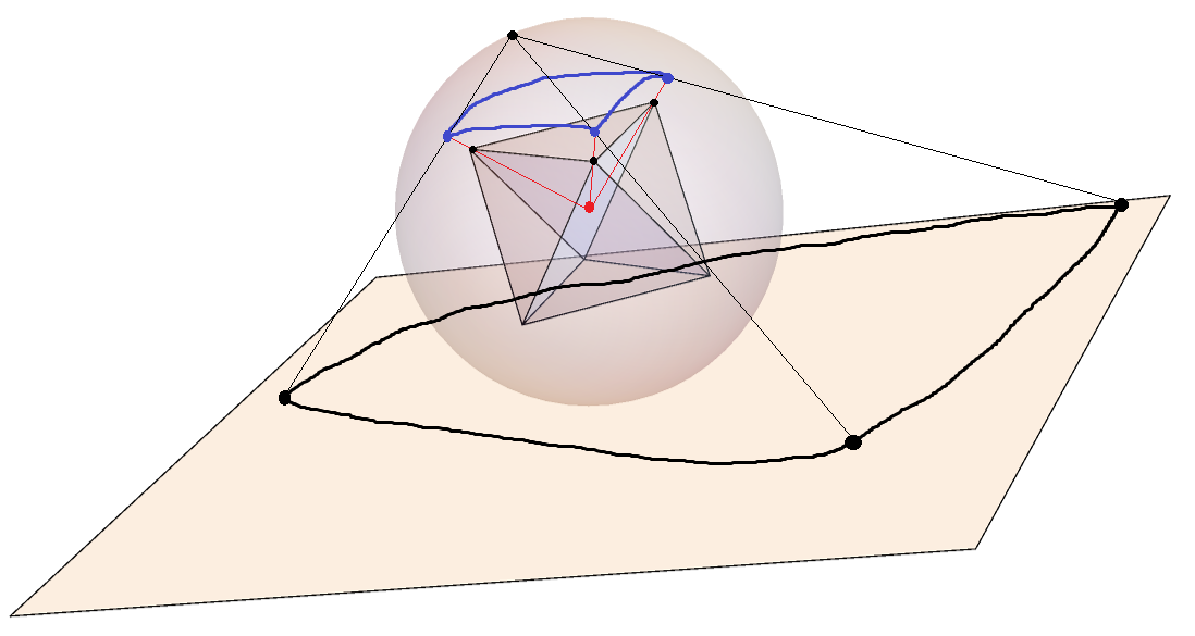
Figure 16: Two bijections from Euler’s theorem about convex polyhedrons.

Corollary 4.

For any face of a planar graph there exists the representation where this face is outer face.

[1em]0em

Proof.

Let’s use the stereographic projection like in the theroem 10 two times. First, let’s project the planar graph from the plane to sphere using inverse stereographic projection with any center. Second, choose the center of second stereographic projection inside the chosen face. By the composition of these projections this face becomes outer face. ∎

Since for polyhedrons the Euler theorem holds then, also upper estimation $\|E\|\leq 3\|V\|-6$ holds. Let’s give lower estimation for polyhedrons. Since the intersection of any two polygons can be just either side of vertex, any vertex degree must be $\geq 3$. Therefore, by using Handshaking lemma $2\|E\|\geq 3\|V\|$ and thus, $1.5\|V\|\leq\|E\|\leq 3\|V\|-6$ holds for polyhedrons.

Definition 8.7.

Platonic solid is a convex polyhedron, that consists of the same regular polygons and the vertices have the same degrees.

Example 8.2.

Let’s $n$ be the number of vertices of polygons of a platonic solid and $deg$ be degree of any vertex. The following holds for platonic solids:

$$n\|F\|=deg\|V\|=2\|E\|.$$

Let’s multiply Euler formula on $2n$ and use the equation below.

$$2n\|V\|-2n\|E\|+2n\|F\|=4n,$$

$$2n\|V\|-n\,deg\|V\|+2\,deg\|V\|=4n,$$

$$\|V\|(2n-deg(n-2))=4n.$$

Since the $n>0$ and $\|V\|>0$, thus $2n-deg(n-2)>0$ and therefore, $(n-2)deg<2n$.

Let’s use this equation and this estimation to classify all platonic solids (see figure 17). Let’s also note that the minimum number of $n=3$ and the minimum degree $deg=3$:

1. $n=3\implies deg<6,$

   1. $deg=3\implies\|V\|=4.$ This platonic solid is called Tetrahedron.

   2. $deg=4\implies\|V\|=6.$ This platonic solid is called Octahedron.

   3. $deg=5\implies\|V\|=12.$ This platonic solid is called Icosahedron.

2. $n=4\implies 2\,deg<8\implies deg<4,$

   1. $deg=3\implies\|V\|=8.$ This platonic solid is called Cube.

3. $n=5\implies 3\,deg<10\implies deg<4,$

   1. $deg=3\implies\|V\|=20.$ This platonic solid is called Dodecahedron.

4. $n\geq 6,$ Let’s use the estimation again:

   $$0>2n-n\,deg-2deg=n(deg-2)-2\,deg)\geq 4\,deg-12.$$

   This gives the contradiction, since $deg\geq 3$.

Using Handshaking lemma and Euler theorem 10 the number of edges and faces can be found. As a result the full classification is obtained:

Name	n	deg	$\|V\|$	$\|E\|$	$\|F\|$
Tetrahedron	3	3	4	6	4
Octahedron	3	4	6	12	8
Icosahedron	3	5	12	30	20
Cube	4	3	8	12	6
Dodecahedron	5	3	20	30	12

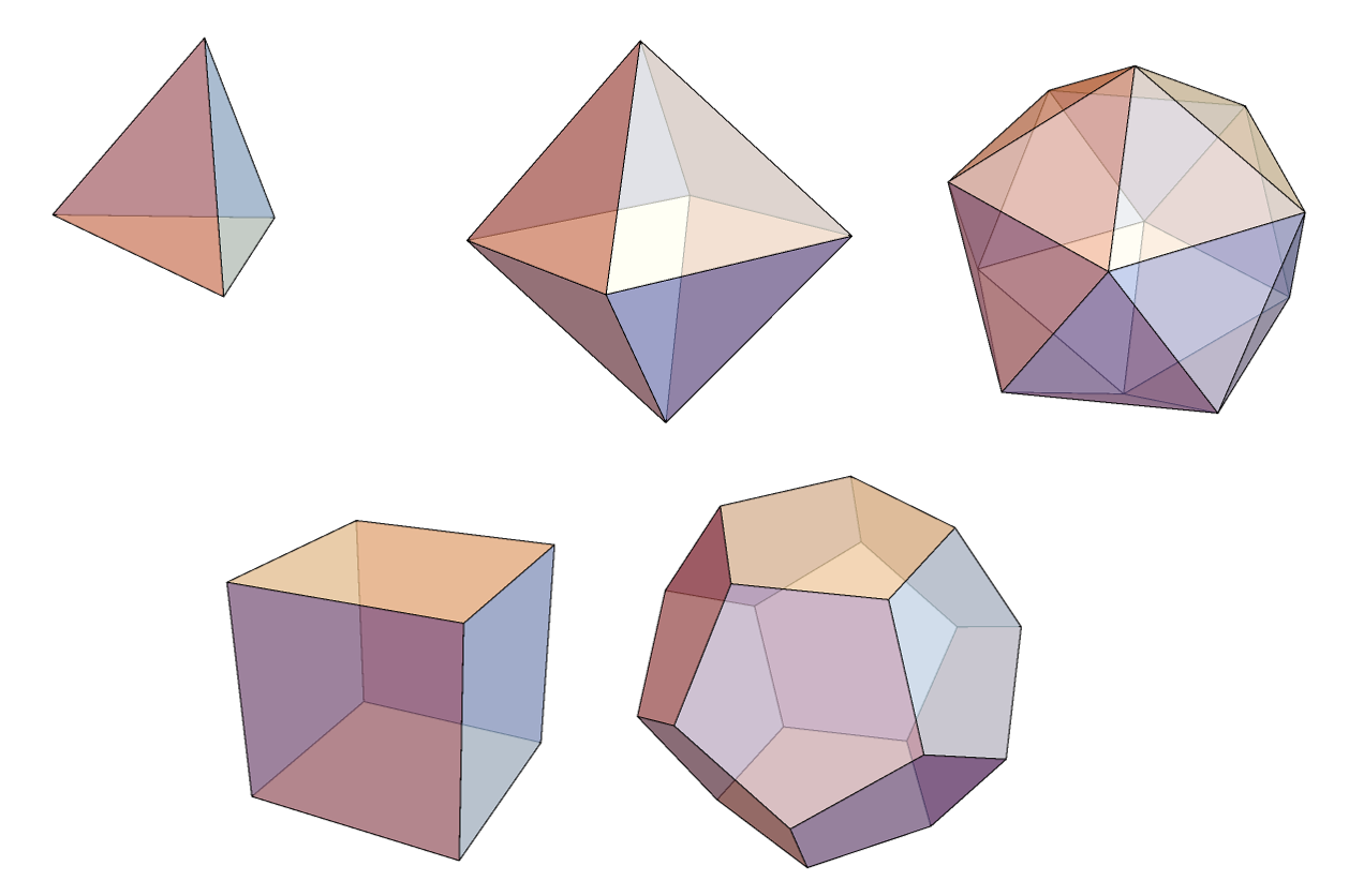
Figure 17: All platonic solids: Tetrahedron, Octahedron, Icosahedron (top), Cube, Dodecahedron (bottom).

9 $K$-connectivity

9.1 $\kappa$-vertex and $\lambda$-edge connectivity

Definition 9.1.

A set of vertices (edges) is called $k$-vertex (edge) cut if a graph becomes not connected after the deletion of this set.

Definition 9.2.

A graph is called $\kappa$-vertex (edge) connected iff. if it doesn’t have any $k-1$-vertex (edge) cuts.

NB! $\kappa$-vertex connectivity is also shortly called $\kappa$-connectivity.

Example 9.1.

1. We assume that empty graph and the graph with only one vertex are not connected.

2. 1-connected graph is just connected.

3. If a graph is $k$-vertex (edge) connected then it is also $k-1$-vertex (edge) connected, $k-2$-vertex (edge) connected and so on.

4. The complete graph $K_{n}$ is $n-1$-vertex and edge connected.

5. The complete bipartite graph $K_{n,m}$ is $\min(n,m)$-vertex and edge connected.

Definition 9.3.

The paths between two vertices are called k-vertex (edge) independent iff. there exist $k$ paths from it which consist of disjoint sets of vertices (edges).

Consider another example:

Statement 1.

Paths between any two vertices of complete graph $K_{d+1}$ are $d$-vertex (edge) independent.

[1em]0em

Proof.

Consider two vertices $v_{i},v_{j}$. Let’s show $d$-vertex (edge) independent paths:

1. One path: $v_{i}v_{j}$.

2. $d-1$ paths: $v_{i}v_{k}v_{j}$, for $v_{k}\in V\setminus\{v_{i},v_{j}\}$.

∎

Theorem (Menger).

A graph is $\kappa$-vertex (edge) connected iff. for any two vertices there exist $\kappa$-vertex (edge) independent paths.

We will proof this theorem in subsection 14.3. Let’s consider the corollary of this theorem:

Corollary 5.

If a graph $G$ is 3-connected then $G\setminus(u,v)$ is 2-connected for any edge $(u,v)$.

We will use this corollary later. Now let’s consider the relation between vertex and edge connectivity:

Lemma 11.

Let $\kappa(G)$, $\lambda(G)$ are numbers of vertex and edge connectivity for a graph $G$ respectively. Let $d(G)$ be the minimum degree. The following holds:

$$\kappa(G)\leq\lambda(G)\leq d(G).$$

[1em]0em

Proof.

1. Case $\kappa(G)\leq\lambda(G)$. Since $\kappa(G)$-vertex independent paths are also edge independent, this estimation holds by the Menger’s theorem.

2. Case $\lambda(G)\leq d(G)$. By deleting $d(G)$ edges at the vertex with minimum degree the graph becomes not connected.

∎

Theorem 11 (($\kappa$, $\lambda$, d)-graph).

For any $\kappa,\lambda,d\in\mathbb{N}:\kappa\leq\lambda\leq d,$ there exists a graph with $\kappa$ — vertex connectivity, $\lambda$ — edge connectivity and $d$ — minimum degree number.

[1em]0em

Proof.

Consider two copies $G_{1},G_{2}$ of complete graph $K_{d+1}$. Let’s mark $\lambda$ vertices in the first graph $G_{1}$ and $\kappa$ vertices in the second $G_{2}$. Add $\lambda$ edges between all marked vertices such that each marked vertex should be adjacent to some added edge (see figure 18 for example). Denote the constructed graph by $G$.

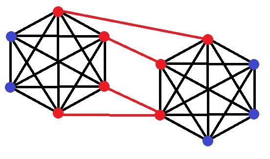
Figure 18: Example of (3, 4, 5)-graph. The red vertices are marked vertices, the red edges are added edges.

Let’s proof, that the graph $G$ is a graph with $\kappa$-vertex connectivity, $\lambda$-edge connectivity and minimal degree $d$.

1. Since $\kappa\leq\lambda<d+1$, there exists unmarked vertex, that remains the same as for complete graph $K_{d+1}$. Hence the minimum degree of graph $G$ equals $d$.

2. Let’s proof that the collection of paths between any two vertices of the graph $G$ is $\kappa$-vertex and $\lambda$-edge independent. If these vertices belong to the same complete sub-graph $K_{d+1}$ then the condition holds from the statement 1. If considered vertices belong to the different complete sub-graphs $K_{d+1}$ then let’s consider following paths: first vertex, any marked vertex from the same sub-graph, adjacent marked vertex from the second sub-graph and the second vertex. It is easy to see that they are vertex and edge independent and the number of paths equals to $\kappa$ and $\lambda$ for vertex and edge independence respectively.

   By using Menger’s theorem the proof ends.

∎

9.2 Bridge detecting algorithm

Definition 9.4.

An edge of a connected graph is called bridge iff. the graph becomes not connected after the deletion of this edge.

NB! The bridges can be only in 1-edge connected graphs.

Let’s consider the bridge detecting algorithm:

Tarjan’s algorithm.

For any vertex $v$ let’s denote by $DFS[v]$ — the order of the vertex $v$, by $a_{v}$ — ancestors of $v$, by $d_{v}$ — descendants of $v$ corresponding to depth first search algorithm.

Description:

1. Use depth first search algorithm to define DFS order $DFS[v]$ and construct the corresponding spanning tree of the graph.

2. For each vertex $v$ in the reverse DFS order define:

   $$low[v]:=min\begin{cases}DFS[v]&\\ DFS[a_{v}]&\text{if edge $(v,a_{v})$ doesn't belong to DFS tree}\\ low[d_{v}]&\text{if edge $(v,d_{v})$ belongs to DFS tree}\end{cases}.$$ (1)

3. The edge $(v,d_{v})$ is a bridge iff. $DFS[v]<low[d_{v}]$.

NB! The complexity of this algorithm is the same as for depth-first search algorithm and equals to $\mathbf{O(\|E\|)}$ for connected graphs.

NB! If one add orientation of the current graph by following: orient DFS tree as Tremaux arborescence and orient other edges from descendants to ancestors, the $low[v]$ will correspond to the lowest number in DFS order that can be reached from the vertex $v$.

Finally, let’s proof:

Lemma 12.

Let the function $low[v]$ is defined by equation 1 for any vertex of a connected graph $G$. The edge $(v,d_{v})$ is a bridge in $G$ iff. $DFS[v]<low[d_{v}]$ for a descendant $d_{v}$ of vertex $v$.

[1em]0em

Proof.

Let’s denote the set of ancestors of $v$ by $A_{v}$ and the set of descendants of $v$ by $D_{v}$. First let’s note that the edge $(v,d_{v})$ is a bridge in $G$ iff. this edge divides vertices by two disjoint sets $A_{v}\bigcup\{v\}$ and $D_{v}$ such that there is no edges between these sets except $(v,d)$. Also the following holds:

$$DFS[a_{v}]<DFS[v]<DFS[d_{v}],\ \forall a_{v}\in A_{v}\text{ and }\forall d_{v}\in D_{v},$$

$$low[v]\leq low[d_{v}],\ \forall d_{v}\in D_{v}.$$

1. Necessarity. Let’s proof that $DFS[v]<low[d_{v}]$ for any descendant $d_{v}$ of vertex $v$ by induction corresponding to inverse DFS order:

   1. Consider the descendant $d_{v}$ with the highest $n=DFS[d_{v}]$. This vertex has no descendants and only can be adjacent to descendants of $v$. Since $DFS[v]<DFS[d],\ \forall d\in D_{v}\implies DFS[v]<DFS[a_{d_{v}}]\implies DFS[v]<low[d_{v}]$.

   2. Let we proof that $DFS[v]<low[d_{v}]$ for any $d_{v}:DFS[d_{v}]\geq k$. Let’s proof it for $d_{v}:DFS[d_{v}]=k-1$. For this $d_{v}:DFS[v]<DFS[d_{v}].$ Since the vertex $d_{v}$ can only be adjacent to descendants of $v$ and $DFS[v]<DFS[d],\ \forall d\in D_{v}\implies DFS[v]<DFS[a_{d_{v}}]$. By the induction: $DFS[v]<low[d_{d_{v}}]$. Therefore, $DFS[v]<low[d_{v}]$.

2. Sufficiency. Assume the contrary: the edge $(v,d_{v})$ is not a bridge. Thus, there exists an edge $(a_{v},d_{1v})$ between two vertices $a_{v}\in A_{v}$ and $d_{1v}\in D_{v}:\text{$d_{1v}$ is descendant of $d_{v}$}$. Thus, $low[d_{v}]\leq low[d_{1v}]\leq DFS[a_{v}]<DFS[v]$ implies contradiction.

∎

Corollary 6.

Let the function $low[v]$ is defined by equation 1 for any vertex of a connected graph $G$. The edge $(v,d_{v})$ is a 1-cut vertex in $G$ iff. $DFS[v]\leq low[d_{v}]$ for a descendant $d_{v}$ of vertex $v$.

[1em]0em

Proof.

The proof is the same as in the previous lemma. ∎

NB! By this corollary Tarjan’s algorithm is also can be used for detecting 1-cut vertices and thus by deleting them one can find all 2-connected components of a graph.

10 Eulerian graph

Definition 10.1.

Eulerian path is a path that walks through every edge of the graph only one time.

Definition 10.2.

Eulerian cycle is an Eulerian path where the first and the last vertices coincide.

Consider the another case of 2-edge connected graph:

Definition 10.3.

An undirected graph is called Eulerian iff. there exists an Eulerian cycle in the graph.

Lemma 13.

An Eulerian graph is 2-edge connected.

[1em]0em

Proof.

Assume the contrary: there exists a bridge $e$ in a graph $G$ such that $G\setminus e$ has at least two connected components. Hence, if there exists Eulerian cycle it should starting and therefore ending in the same component. This holds the contradiction. ∎

Theorem 12 (Necessary and sufficient condition for Eulerian graph).

An undirected graph is Eulerian iff. it is connected and degrees of all vertices are even.

[1em]0em

Proof.

1. Necessarity. The Eulerian graph is connected. Assume the contrary: there exists a vertex with odd degree. Let’s delete the edges of the current graph one by one through the Eulerian cycle. Since we go in to the vertex by one edge and go out from this vertex by another edge, each time after visiting a vertex the degree of this vertex decreased by 2, and hence the parity of this vertex degree remains the same (note that it also holds to the starting vertex because of the cycle). Therefore, after the deleting all edges corresponding to Eulerian cycle (all edges in the graph) the parity of all vertices remains the same. It holds the contradiction with existence the vertex with odd degree.

2. Sufficiency. Let’s start any walk at our graph $G$ with deleting visiting edges. This walk ends in our starting vertex (the first and last vertices in the walk have odd degrees every time and if vertex has odd degree there exists an edge adjacent to this vertex). Therefore, when the walk ends, this walk will form a cycle. Let’s denote the set of edges of this cycle by $C_{1}$.

   Consider the graph $G\setminus C_{1}$. Do the same procedure and find the set of edges $C_{2}$ of a new cycle in $G\setminus C_{1}$ and so on. Let’s denote the set of this sets by $C={C_{i}}$. Since all vertices have even degree, the set $C$ contains every edge of $G$. Let’s construct the Eulerian cycle by using a stack $S$ and the set $C$:

   1. Start from any vertex of $C_{1}$. Take away $C_{1}$ from $C$ and add it to the stack $S$.

   2. Go through an edge corresponding to this cycle in the top of the stack $S$. If there is no edges corresponding to this cycle, delete the cycle from $S$ and do 2b again.

   3. If there exists an edge corresponding to a cycle $C_{i}$ from $C$, take away $C_{i}$ from $C$, add it to the stack $S$ and go to 2b.

   This algorithm produces Eulerian cycle in the graph $G$.

∎

Theorem 13 (Eulerian path existence).

An Eulerian path exists in the connected graph iff. there exist no more than two vertices with odd degrees.

[1em]0em

Proof.

1. Assume that there are no odd vertices, then there exists Eulerian cycle by the theorem 12.

2. Assume that there are only two vertices with odd degrees $u$ and $v$.

   1. If there exists an edge $(u,v)$ then after deleting this edge the graph will have no odd vertices and contains Eulerian cycle by the theorem 12. This Eulerian cycle with the edge $(u,v)$ forms the Eulerian path.

   2. If there are no edges between $u$ and $v$, add the edge $(u,v)$ to the graph. Therefore, the graph with $(u,v)$ will have no odd vertices and contains Eulerian cycle by the theorem 12. This Eulerian cycle without the edge $(u,v)$ forms the Eulerian path.

∎

NB! If there are only two vertices with odd degrees in the graph, an Eulerian path will starts and ends in these two vertices.

Consider basic Eulerian cycle searching algorithms in connected graphs:

1. Fleury’s algorithm.
   This algorithm used the algorithm of testing whether the graph will become not connected after the deleting current edge.
   Description:

   1. Walk in the graph with deleting visiting edges which keep the graph connected.

   2. If all adjacent edges provided the graph to be not connected (all edges are bridges) go through one of these edges and delete. Do 1a again.

   NB! By using Tarjan’s algorithm for detecting bridges the complexity of Fleury’s algorithm will be $\mathbf{O(\|E\|^{2})}$.

2. Using list structure.
   This algorithm is based on the algorithm introduced in the theorem 12.
   Description:

   1. Construct the set $C$ from the theorem 12 and mark all edges of the graph corresponding to cycles $C_{i}$.

   2. Add vertices of $C_{1}$ to the list $L$ and start from the top.

   3. Go to the next vertex in $L$. If there exist an edge $e$ adjacent to this vertex not in the list $L$ and corresponded to a cycle $C_{i}$, add all vertices of $C_{i}$ starting with this edge in the current position of the list $L$. Do 2c again.

   In the end the list will contain Eulerian cycle.

   NB! The complexity of this algorithm is $\mathbf{O(\|E\|\,\|V\|)}$.

3. Using two stacks.
   This algorithm used two stack structures $S_{1}$ and $S_{2}$.
   Description:

   1. Walk in the graph with deleting visiting edges and add consecutive vertices corresponded to these edges to the stack $S_{1}$ until it is possible.

   2. Transfer the vertex $v$ in top of the stack $S_{1}$ to the stack $S_{2}$. Do 3a again starting with the new vertex in the top of the stack $S_{1}$.

   In the end the stack $S_{2}$ will contain Eulerian cycle.

   NB! The complexity of this algorithm is $\mathbf{O(\|E\|\,\|V\|)}$.

11 Hamiltonian graph

Definition 11.1.

Hamiltoinian cycle is a simple cycle that consist of all vertices of a graph.

Definition 11.2.

A graph is called Hamiltonian iff. there exists a Hamiltoinian cycle in the graph.

Lemma 14.

Planar graph $G$ is Hamiltonian iff. there exist a representation and a simple cycle $C$ such that the parts of the dual graph $D(G)$ which belong to $int(C)$ and $out(C)$ are trees.

[1em]0em

Proof.

We will proof this lemma in the subsection 13.1. ∎

In the general case it is not very easy to give necessary and sufficient conditions for Hamiltoinian graphs, here we introduce the simplest ones:

Lemma 15 (Necessary Hamiltonian condition).

A Hamiltonian undirected graph is 2-connected.

[1em]0em

Proof.

Assume the contrary: there exists a vertex $v$ in a graph $G$ such that $G\setminus v$ has at least two connected components. Hence, if there exists Hamiltonian cycle it should starting and therefore ending in the same component. This holds the contradiction. ∎

NB! In general situation the construction of Hamiltonian cycle is NP-hardness problem. Thus knowledge of the Hamiltonian cycle in a graph is used in cryptography namely in the zero-knowledge protocol.

Lemma 16.

Graphs of platonic solids are Hamiltonian.

[1em]0em

Proof.

The proof is in figure 19. ∎

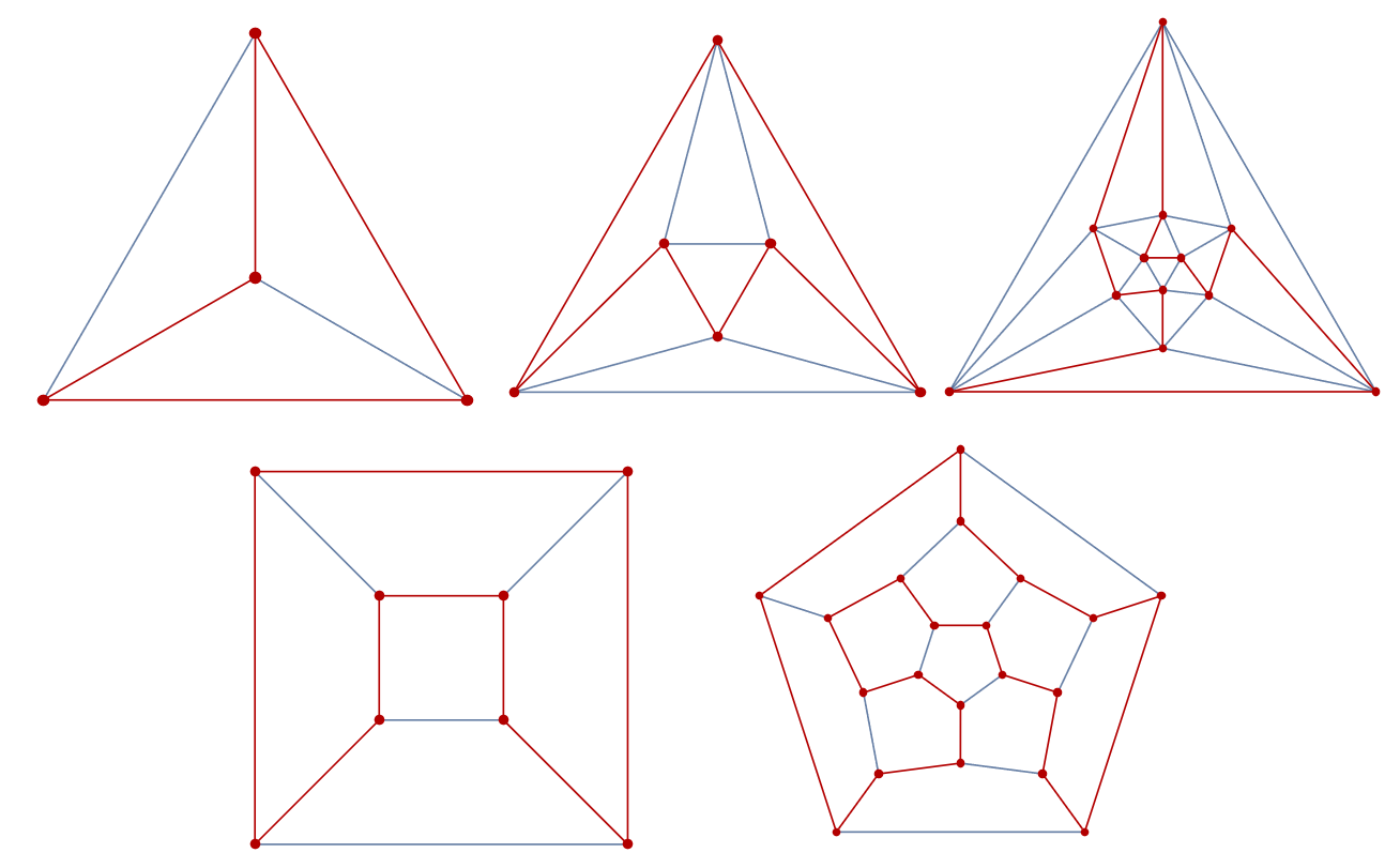
Figure 19: Hamiltonian cycles in graphs of Platonic solids.

Let’s introduce several sufficient conditions of Hamiltonian graphs:

Theorem 14 (Ore).

Let’s $\|V(G)\|=n$, then

$$\deg(u)+\deg(v)\geq n,\,\forall\text{ not adjacent }u,v\in V(G)\implies G\text{ is Hamiltonian.}$$

[1em]0em

Proof.

Let’s assume the contrary: there exists not Hamiltonian graph $G$ that is satisfied the condition. By the adding edges to the graph $G$ one can obtain a Hamiltonian graph. Let $G^{\prime}$ be the boundary case: $G^{\prime}$ is not Hamiltonian graph and $G^{\prime}\bigcup(u,v)$ — Hamiltonian. The condition of this theorem also holds for the graph $G^{\prime}$, and the edge $(u,v)$ is the edge of Hamiltonian cycle in $G^{\prime}\bigcup(u,v)$ (otherwise $G^{\prime}$ is Hamiltonian). Let $w_{n}$ is the next vertex for $w$ by the Hamiltonian cycle. Let $V^{\prime}\subset V(G^{\prime})$ be the set of vertices $w\in V^{\prime}$ such that $(v,w)$ is an edge in $G^{\prime}$ and $U^{\prime}\subset V(G^{\prime})$ be the set of vertices $w\in U^{\prime}$ such that $(u,w_{n})$ is an edge in $G^{\prime}$.

$$\|U^{\prime}\|=\deg(u),\ \|V^{\prime}\|=\deg(v),$$

$$U^{\prime}\cup V^{\prime}\subset V(G^{\prime})\setminus\{v\}\implies\|U^{\prime}\cup V^{\prime}\|\leq n-1,$$

$$\|U^{\prime}\cup V^{\prime}\|=\|U^{\prime}\|+\|V^{\prime}\|+\|U^{\prime}\cap V^{\prime}\|,$$

$$\|U^{\prime}\|+\|V^{\prime}\|=\deg(u)+\deg(v)\geq n\implies\|U^{\prime}\cap V^{\prime}\|\geq 1.$$

Thus there exists a vertex $w$ such that the edges $(v,w)$ and $(u,w_{n})$ are in the graph $G$. This holds contradiction, see figure 20.

∎

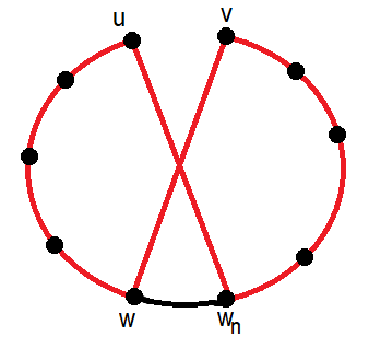
Figure 20: Hamiltonian cycle in the case $\|U^{\prime}\cap V^{\prime}\|\geq 1$ in the Ore’s theorem 14.

NB! This theorem has been proved for undirected graphs but it can be proved also for directed case in the same way.

Theorem 15 (Dirac).

Let’s $\|V(G)\|=n$, then

$$\deg(u)\geq\frac{n}{2},\,\forall u\in V(G)\implies G\text{ is Hamiltonian.}$$

[1em]0em

Proof.

It simply holds from previous theorem. ∎

NB! For directed graph this theorem also the same.

To prove the next Bondy–Chvátal theorem first several definitions and lemmas are needed:
Let’s denote the number of vertices of our graph $G$ by $n$.

Definition 11.3.

The sequence of degrees $d_{i}=deg(v_{i})$ is called ordered sequence of degrees iff. $d_{1}\leq d_{2}\leq...\leq d_{n}$ for some re-numeration of the vertices.

Definition 11.4.

An ordered sequence of degrees $d_{i}$ is majorized by an ordered sequence of degrees $d^{\prime}_{i}$ iff. $d_{i}\leq d^{\prime}_{i}$ for $i=1...n$

From this point let consider the numeration of $G$ such that the sequence of degrees $G$ is ordered.

Statement 2 (Majorized sequance).

Let a graph $G^{\prime}$ is obtained from a graph $G$ by adding one edge. Then the ordered sequence of degrees $G^{\prime}$ majorizes the ordered sequence of degrees $G$.

[1em]0em

Proof.

Let’s the added edge be $(v_{i},v_{j}),i<j$. Then new degrees of vertices $v_{i}$ and $v_{j}$ will be $d_{i}+1$ and $d_{j}+1$. Let’s prove that after changing $d_{i}$ to $d_{i}+1$ one can re-numerate vertices such that new ordered sequence $d^{\prime}_{i}$ will majorize previous one.

Let the number $p\in\mathbb{Z}^{+}$ is defined as following: $d_{i}=d_{i+1}=...=d_{i+p}<d_{i+p+1}$.

Now let’s produce the re-numeration:

$$d^{\prime}_{k}=d_{k},\ k=1,2,...,\hat{i+p},...n\quad\text{ and }\quad d^{\prime}_{i+p}=d_{i+p}+1.$$

The proof ends by doing the same procedure for $d_{j}$. ∎

Lemma 17 (Upper estimation).

$$d_{k}\leq k\iff\|{v\in V(G):\deg(v)\leq k}\|\geq k.$$

[1em]0em

Proof.

1. $(\Rightarrow).$

   $$d_{k}\leq k\Rightarrow d_{1}\leq d_{2}\leq...\leq d_{k}\leq k\Rightarrow\|{v\in V(G):\deg(v)\leq k}\|\geq k.$$

2. $(\Leftarrow).$

   $$\|{v\in V(G):\deg(v)\leq k}\|=k+p,\ p\geq 0\Rightarrow d_{1}\leq d_{2}\leq...\leq d_{k}\leq...\leq d_{k+p}\leq k\Rightarrow d_{k}\leq k.$$

∎

The same poof for

Lemma 18 (Lower estimation).

$$d_{n-k}\geq n-k\iff\|{v\in V(G):\deg(v)\geq n-k}\|\geq k+1.$$

[1em]0em

Proof.

1. $(\Rightarrow).$

   $$d_{n-k}\geq n-k\Rightarrow n-k\leq d_{n-k}\leq d_{n-k+1}...\leq d_{n}\Rightarrow\|{v\in V(G):\deg(v)\geq n-k}\|\geq k+1.$$

2. $(\Leftarrow).$

   $$\|{v\in V(G):\deg(v)\geq n-k}\|\geq k+p+1,\ p\geq 0\Rightarrow$$

   $$\qquad\qquad\qquad\qquad\Rightarrow n-k\leq d_{n-k-p}\leq d_{n-k-p+1}...\leq d_{n-k}\leq...\leq d_{n}\Rightarrow d_{n-k}\geq n-k.$$

∎

Lemma 19 (Implication and majorized sequence).

If the following implication holds for the sequence of degrees $d_{i}$:

$$d_{k}\leq k<\frac{n}{2}\implies d_{n-k}\geq n-k,$$

then it also holds for a majorized sequence of degrees $d^{\prime}_{i}$.

[1em]0em

Proof.

1. If $d_{k}\leq k<d^{\prime}_{k}$ then implication holds by the false first argument,

2. If $d_{k}\leq d^{\prime}_{k}\leq k$ then $n-k\leq d_{n-k}\leq d^{\prime}_{n-k}$ by the majorization property.

∎

Theorem 16 (Bondy–Chvátal).

If for an ordered sequence of degrees of a connected graph $G$ the implication holds:

$$d_{k}\leq k<\frac{n}{2}\implies d_{n-k}\geq n-k,$$

then $G$ is Hamiltonian.

[1em]0em

Proof.

Assume the contrary: there exists a graph $G$ that satisfies the condition of the theorem. Let $G^{\prime}$ be the maximal non Hamiltonian graph by adding the edges to the graph $G$. Thus $G^{\prime}$ becomes Hamiltonian by adding any edge. Let’s $u$ and $v$ be two not adjacent vertices such that $\deg(u)+\deg(v)$ is maximal in $G^{\prime}$ and let $\deg(u)\leq\deg(v)$ without loss of generality.

The graph $G^{\prime}\bigcup(u,v)$ is Hamiltonian. Let like in the Ore’s theorem 14 $w_{n}$ is the next vertex for $w$ by the Hamiltonian cycle. Let $V^{\prime}\subset V(G^{\prime})$ be the set of vertices $w\in V^{\prime}$ such that $(v,w)$ is an edge in $G^{\prime}$ and $U^{\prime}\subset V(G^{\prime})$ is the set of vertices $w\in U^{\prime}$ such that $(u,w_{n})$ is an edge in $G^{\prime}$. Then,

$$\|U^{\prime}\|=\deg(u),\ \|V^{\prime}\|=\deg(v),$$

$$U^{\prime}\cup V^{\prime}\subset V(G^{\prime})\setminus\{v\}\implies\|U^{\prime}\cup V^{\prime}\|\leq n-1,$$

1. If $\|U^{\prime}\cap V^{\prime}\|\geq 1$, then it holds the contradiction like in the Ore’s theorem 14 by figure 20.

2. If $\|U^{\prime}\cap V^{\prime}\|=0$. Let’s denote $\deg(u)$ by $k$.

   $$2k=2\deg(u)\leq\deg(u)+\deg(v)=\|U^{\prime}\cup V^{\prime}\|\leq n-1<n\implies k<\frac{n}{2}.$$

   Then $\forall w\in U^{\prime}$:

   1. $w$ doesn’t adjacent to $v$,

   2. $\deg(w)\leq\deg(u)=k$ (otherwise $\deg(w)+\deg(v)>\deg(u)+\deg(v)$).

   Therefore,

   $$\|z\in V(G):\deg(z)\leq k\|\geq\|U^{\prime}\|=\deg(u)=k\overset{\text{upper estimation}}{\implies}d_{k}\leq k<\frac{n}{2}\overset{\text{cond. of theorem}}{\implies}$$

   $$d_{n-k}\geq n-k\overset{\text{lower estimation}}{\implies}\|z\in V(G):\deg(z)\geq n-k\|\geq k+1,$$

   and thus there exists vertex $z$ not adjacent to $u$ with $\deg(w)\geq n-k$. For this vertex $\deg(z)+\deg(u)\geq n>\deg(v)+\deg(u)$. This holds a contradiction.

∎

Theorem 17 (Whitney).

Any planar 4-connected graph is Hamiltonian.

[1em]0em

Proof.

We will prove this theorem later in the subsection 12.2 ∎

12 Planarity and $\kappa$-connectivity

12.1 3-connected graph

Definition 12.1.

$C$-component of the graph $G$ corresponded to a simple cycle $C$ is either edge that doesn’t belong to the cycle $C$ but adjacent to vertices of $C$ or connected component of the graph $G\setminus C$ with all attachments from this sub-graph to the cycle $C$.

Definition 12.2.

Two $C$-components are skew iff. they contains simple paths with starting points $x_{1},x_{2}\in C$ and ending points $y_{1},y_{2}\in C$ such that the vertices are in the order $x_{1},x_{2},y_{1},y_{2}$ corresponded to some orientation of the cycle $C$.

Lemma 20.

The minimum non-planar sub-graph of a non-planar graph is 2-connected.

[1em]0em

Proof.

Let’s denote this sub-graph by $G$.

1. Let’s proof that $G$ is 1-connected of just connected. Assume the contrary. Then, this sub-graph $G$ has at least two connected components. Since $G$ is minimum non-planar, then, each component should be planner and therefore, sub-graph $G$ is also planar. This holds contradiction.

2. Let’s proof that $G$ is 2-connected. Assume the contrary. Then, there exists a vertex $v$, such that by deleting $v$ graph becomes not connected and thus has at least two connected components. Let’s denote one of the components by $G_{1}$ and by $G_{2}$ all the rest. Since the sub-graph $G$ is minimum non-planar, then, the maximum sub-graphs on $V(G_{1})\bigcup\{v\}$ vertices and on $V(G_{2})\bigcup\{v\}$ vertices are planar. By using corollary 4 one can modify the representations of these sub-graphs such that vertex $v$ would belong to the boundary of the outer faces of these sub-graphs. Therefore, the union of representations of these sub-graphs is planar and is representation of sub-graph $G$. This holds contradiction.

∎

Lemma 21.

If the minimum non-planar sub-graph of a non-planar graph doesn’t contain subdivisions of complete graphs $K_{5}$ and $K_{3,3}$ then this sub-graph is 3-connected.

[1em]0em

Proof.

Let’s assume the contrary. Denote the minimum non-planar sub-graph by $G$. By lemma 20 the sub-graph $G$ is 2-connected, then, there exist two vertices $u$ and $v$, such that by deleting them $G$ becomes not connected. Let’s denote the connected components of the $G\setminus\{u,v\}$ by $H_{1},H_{2},...,H_{k}$.

Let’s $M_{i}$ be the connected sub-graph on vertices $V(H_{i})\bigcup\{u,v\}$. Let’s prove that each $M_{i}$ is also connected. Assume the contrary: $M_{i}$ is not connected. Thus, $M_{i}\setminus(u,v)$ has connections to only one vertex. Let this vertex be $v$ without loss of generality. Then, if one delete this vertex $v$, the graph $G$ becomes not connected. This contradict to the 2-connectivity property of $G$. Therefore, each $M_{i}$ has connections to both vertices $u$ and $v$ and thus, connected.

Assume that all $M_{i}+(u,v)$ are planar, then one can combine them for a whole planar representation by putting them inside each other (see figure 21). Therefore, $\bigcup_{i=1}^{k}(M_{i}+(u,v))=G+(u,v)$ is planar. This contradict with non-planarity of $G$. Thus, there exists non-planar $M_{i}+(u,v)$.

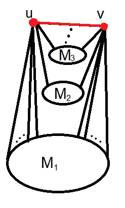
Figure 21: Planar representation of $\bigcup_{i=1}^{k}(M_{i}+(u,v))$ for lemma 21.

Since $G$ is the minimum non-planar sub-graph that contains no subdivisions of graphs $K_{5}$ and $K_{3,3}$, the graph $M_{i}+(u,v)$ should contain subdivisions of graphs $K_{5}$ and $K_{3,3}$. Since all $M_{i}$ are connected, for any $j\neq i$ there exists path $P_{uv}$ between $u$ and $v$ in $M_{j}$ and therefore, $M_{i}\bigcup P_{uv}\subset G$ contains subdivisions of graphs $K_{5}$ and $K_{3,3}$. This holds contradiction since $G$ is not contains subdivisions of graphs $K_{5}$ and $K_{3,3}$. ∎

Now let’s prove the Pontryagin-Kuratowski theorem:

Theorem 18 (Pontryagin-Kuratowski).

A connected graph is planar iff. it doesn’t contain subdivisions of complete graphs $K_{5}$ and $K_{3,3}$.

[1em]0em

Proof.

Necessarity holds from lemma 9 and 10.
Sufficiency. Assume the contrary: there exists non-planar graph that doesn’t contain subdivisions of complete graphs $K_{5}$ and $K_{3,3}$. Let’s consider it’s minimum non-planar sub-graph $G$. By lemma 21 this sub-graph $G$ is 3-connected.

Consider two adjacent vertices $u$ and $v$. Since $G$ is minimum non-planar sub-graph, $G^{\prime}=G\setminus(u,v)$ is planar. By corollary 5 the graph $G\setminus(u,v)$ is at least 2-connected and by Menger’s theorem there exist two vertex independent paths from $u$ to $v$. Thus, there exists a simple cycle in planar representation of $G^{\prime}$ that contains vertices $u$ and $v$. Let $C$ be the simple cycle that contains $u$ and $v$ in planar representation of $G^{\prime}$ with the maximum edges in $int(C)$.

If there exists a vertex that belongs to the $out(C)$ one can construct the cycle that contains more edges in inner part than in $int(C)$ (see figure 22). Thus all vertices of the planar representation $G\setminus(u,v)$ belongs to $int(C)$.

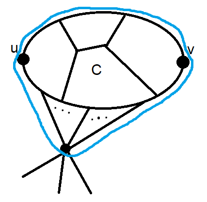
Figure 22: The cycle (blue) with more edges in inner part than in $int(C)$.

Let’s give some additional definitions which are necessary for the proof: let’s denote by bridge of cycle $C$ in planar representation of $G^{\prime}$ a simple path starting and ending in vertices of $C$ that doesn’t contain another vertices and edges of $C$ (this “bridge of cycle” definition is not general definition in graph theory we use this definition only in this theorem. The general another definition of a bride will be introduced in section 9.2.). If bridge laying in $out(C)$ then it is called outer bridge, if it is in $int(C)$ then it is called inner bridge.

Let’s consider a $C$-component in planar representation of $G^{\prime}$. Since the sub-graph $G$ is connected and all another vertices belongs to $int(C)$ then all connected components of $G^{\prime}\setminus C$ are inner $C$-components.

Now we done all preparation for the proof. Let’s prove by steps:

1. If there is no inner (outer) bridges in $G^{\prime}$ then there exists planar representation of $G$. This holds a contradiction, thus there exist at least one inner and one outer bridge.

2. If all inner bridges in $G^{\prime}$ are not skew with $(u,v)$ then also there exists planar representation of $G$. This holds a contradiction, thus at least one inner bridge is skew with $(u,v)$. Let’s denote this inner bridge by $B_{1}$.

3. Since there is no vertices belongs to $out(C)$ then all outer bridges are edges.

4. If there exists an outer bridge in $G^{\prime}$ that is not skew with $(u,v)$ one can expand the cycle $C$ such that it will contain more edges (like in figure 22). This holds a contradiction, thus all outer bridges are skew with $(u,v)$. Let’s denote an outer bridge by $B_{2}$.

5. Any two inner $C$-components are not skew otherwise they intersect and form one $C$-component.

6. If a $C$-component is skew with $(u,v)$ and outer bridge then $G$ contains a subdivision of $K_{3,3}$ (see figure 23 left). This holds a contradiction, thus any $C$-component are not skew with any outer bridge.

7. If there doesn’t exist bridges from $u$ to $v$. Then, there exists a planar representation of $G$: by transferring outer edges (outer $C$-components) to $int(C)$ and inner $C$-components which are not skew to the edge $(u,v)$ to $out(C)$ (see figure 23 right). This holds a contradiction, thus there exists a bridge from $u$ to $v$. Let’s denote it by $B_{3}$.

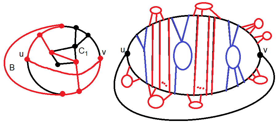
Figure 23: The subdivision of $K_{3,3}$ red for the case 6 in the theorem (left). $C$-component denoted by $C_{1}$ and outer edge by $B$. The planar representation of the sub-graph $G$ for the case 7 (right). Inner $C$-components which are skew to $(u,v)$ marked as blue, and transferred outer edges and inner $C$-components which are not skew to $(u,v)$ marked as red.

Since the sub-graph $G^{\prime}$ is planar the bridge $B_{1}$ should intersects with $B_{3}$ in some points. Consider the cases of relative positions of $B_{1}$, $B_{2}$ and $B_{3}$:

1. The bridges $B_{1}$ and $B_{2}$ don’t intersect.

2. The bridges $B_{1}$ and $B_{2}$ intersect in 1 point.

3. The bridges $B_{1}$ and $B_{2}$ intersect at least in 2 points.

And

1. Bridges $B_{1}$ and $B_{3}$ intersect in 1 point.

2. Bridges $B_{1}$ and $B_{3}$ intersect at least in 2 points.

For cases 1ab, 2ab and 3b the sub-graph $G$ contains a subdivision of $K_{3,3}$ (see figure 24). For the case 3a it is easy to see that the sub-graph $G$ contains a subdivision of $K_{5}$. This holds the contradiction and ends the proof.

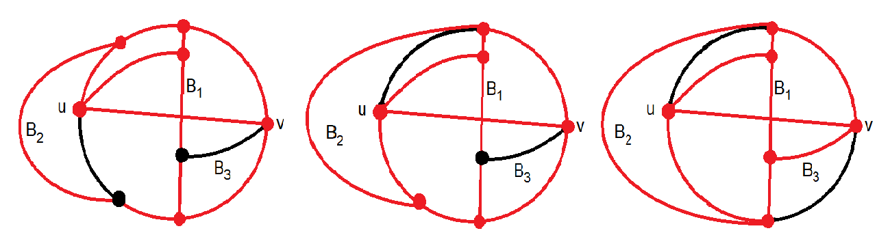
Figure 24: The subdivisions of $K_{3,3}$ marked as red for the cases 1ab (left), 2ab (middle), 3b (right) in the theorem.

∎

Another result corresponding to connections between planarity and connectiveness is

Theorem (Steinitz).

A connected graph is planar and 3-connected iff. it is a graph of a convex polyhedron.

We will proof this theorem in subsection 13.2.

12.2 4-connected graph

Theorem 19 (Thomassen).

Let $C_{out}$ be a cycle corresponded to outer face of 2-connected planar graph $G$. Consider a vertex $v$ and an edge $e$ of $C_{out}$ and any another vertex $u$. Then there exists simple cycle $C$ that contains $u,v$ and the edge $e$ such that

1. Each $C$-component has at most 3 vertices of attachments,

2. Each $C$-component containing an edge of $C_{out}$ has at most 2 vertices of attachments.

Corollary 7.

(Whitney). Any planar 4-connected graph is Hamiltonian.

[1em]0em

Proof.

Since the outer face should contain at least 3 vertices, let’s choose an edge $e\in C_{out}$ not adjacent to $v\in C_{out}$ and $u\notin C_{out}$. The simple cycle $C$ corresponded to Thomassen theorem 19 should be Hamiltonian cycle (otherwise there exists $C$-component with $\|V(C)\|\geq 1$ that has at most 3 attachments and it holds a contradiction with 4-connectivity). ∎

12.3 Planarity testing algorithms

By using Tarjan’s algorithm one can delete all 1-cut vertices in a graph and consider just 2-connected components. Therefore, consider a 2-connected graph without loss of generality.

Definition 12.3.

Interplacement graph with respect to cycle $C$ is the graph where vertices correspond to $C$-components of the cycle $C$ and edges correspond to the skew relationship between $C$-components (see figure 25 for example).

NB! Interpacement graph can have isolated vertices.

Here we will consider the bipartitness property for not connected graphs: not connected graph is said to be bipartite if each connected component of the graph is bipartite (see figure 25).

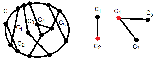
Figure 25: The simple cycle $C$, five $C$-components $C_{1},C_{2},...,C_{5}$ (left) and bipartite interplacement graph with respect to cycle $C$ (right).

Consider the basic algorithm for testing planarity property for 2-connected graphs:

1. Auslander-Parter algorithm.
   This algorithm is testing planarity property of 2-connected graph $G$ by checking interplacement graphs for each cycle $C$ for bipartitness.
   Description:

   1. Find any simple cycle $C$, e.g. by adding an edge to spanning tree.

   2. Find all connected components of the graph $G\setminus C$ and add to them edges which doesn’t belong to the cycle $C$ but adjacent to vertices of $C$. These will be all $C$-components.

   3. Construct interplacement graph and check it for bipartitness. If interplacement graph is no bipartite, the graph $G$ is not planar.

   4. For each $C$-component $C^{\prime}$ construct a new cycle in the sub-graph $G^{\prime}=C\bigcup C^{\prime}$ by changing the path on $C$ between any two consecutive (corresponding to some direction on $C$) attachments of $C^{\prime}$ to the path between them in $C^{\prime}$ (see figure 26) and go recursively to the step 1b for the graph $G^{\prime}$.

   5. The recursion terminates when the cycle $C$ has just one $C$-component in $G^{\prime}$ and it is a path.

   

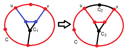
   Figure 26: The simple cycle $C$ (left, red), $C$-component $C_{1}$ (left, black and blue) and a path between consecutive attachments of $C_{1}$ through $C$-component $C_{1}$ (left, blue). New cycle $C$ (right, red) and new $C$-components $C_{2},C_{3}$ (right, black) corresponded to the step 1d of Auslander-Parter algorithm.

   Lemma 22.

   A 2-connected graph is planar iff. for each simple cycle $C$:

   1. the interplacement graph is bipartite,

   2. for each $C$-component $C^{\prime}$ the sub-graph $C\bigcup C^{\prime}$ is planar.

   [1em]0em

   Proof.

   If all the condition hold then planar representation can be constructed by reverse steps of recursion in Auslander-Parter algorithm. ∎

   NB! If a graph is planar (if it is not the algorithm terminates earlier) the number of vertices which belong to $int(C)$ decreased each step of the recursion, hence the depth of recursion is $O(\|V\|)$. Since the graph is planar, $\|E\|\leq 3\|V\|-6$ and thus, the number of $C$-components (and vetrices of an interplacement graph) is $O(\|E\|)=O(\|V\|)$. Therefore, the complexity of bipartite testing algorithm for the interplacement graph is $O(\|V\|^{2})$. Thus, the complexity of Auslander-Parter algorithm is $\mathbf{O(\|V\|^{3})}$.

13 Duality

13.1 Dual graphs

Definition 13.1.

Dual graph $D(G)$ for a planar representation of a graph $G$ is the graph constructed as following: in each face $F_{u}$ of a graph $G$ the corresponded vertex $u$ of dual graph is added, if two faces $F_{u}$ and $F_{v}$ adjacent to each other, then the edge $(u,v)$ of dual graph is added.

NB! Dual graph can contain loops and multi-edges (see figure 27).

NB! For isomorphic graphs dual graphs can be non-isomorphic (see figure 27 left).

NB! Non-isomorphic graphs can have isomorphic dual graphs (see figure 27 right).

Since the dual graph can be not simple, in this section we also consider 1-cycles (loops) and 2-cycles (from multi-edges) as simple-cycles. Also we consider the planar representations for not only simple graphs.

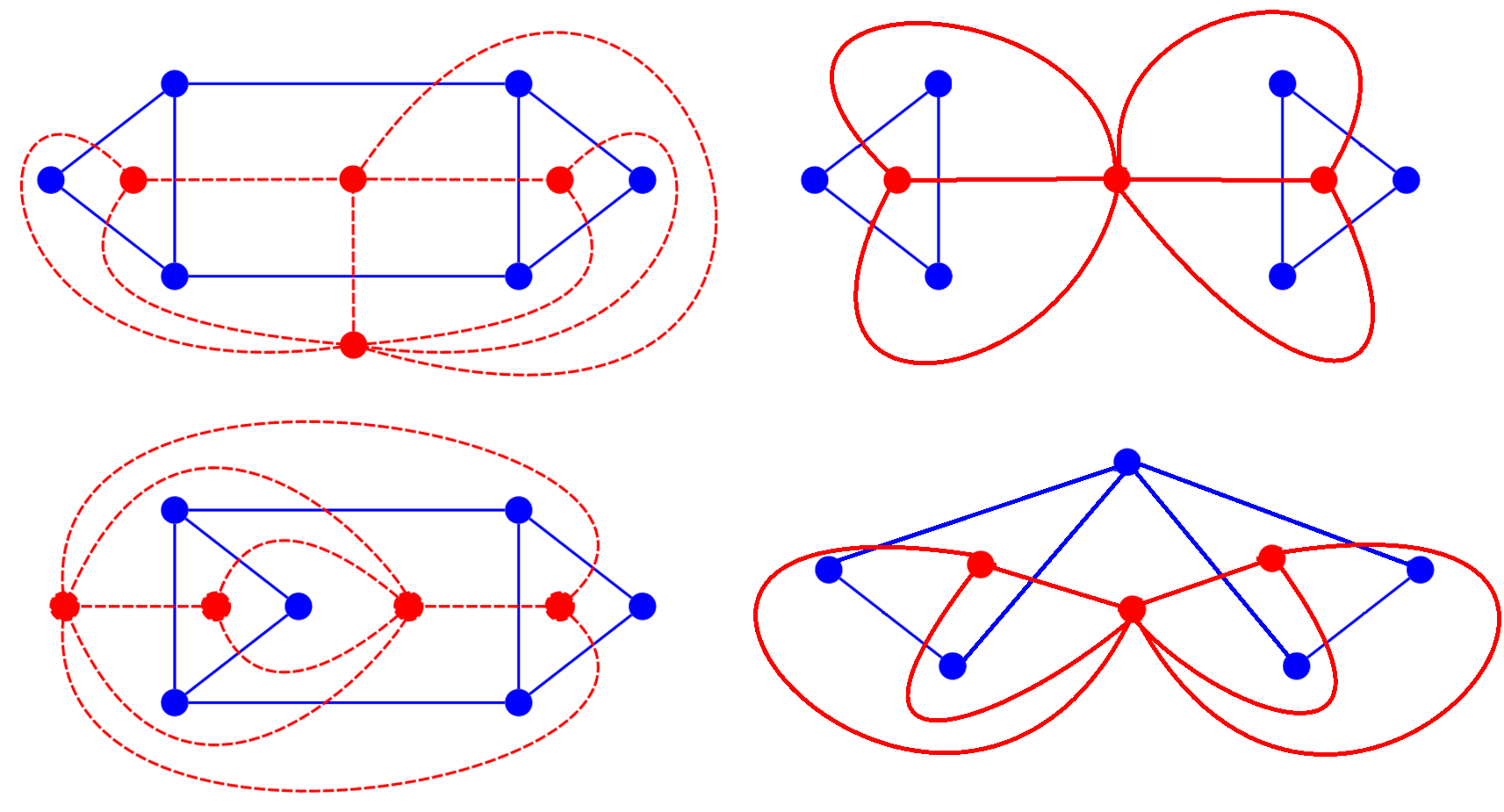
Figure 27: Not isomorphic dual graphs for two different planar representations of one simple graph (left). Isomorphic dual graphs for non-isomorphic simple graphs (right).

Lemma 23.

The dual graph $D(G)$ is always connected.

[1em]0em

Proof.

For any two vertices in $D(G)$ there exists curve starting from first point and ending in second point. The sequence of faces and edges traversed by this curve corresponds to the path between these two points. ∎

Lemma 24.

The dual graph is planar.

[1em]0em

Proof.

Any edge of dual $(u,v)$ corresponds to the adjacency property of two faces $F_{u}$ and $F_{v}$ and thus corresponds to the edge of the graph $G$ that belongs to $F_{u}\bigcap F_{v}$. Therefore, one can redraw this representation of the dual graph such that $u\in int(F_{u})$ and $v\in int(F_{v})$ and $(u,v)\subset F_{u}\bigcup F_{v}$ and moreover there exists small neighborhood $U(u,v)\subset F_{u}\bigcup F_{v}$.

Assume the contrary, that dual graph is not planar. Then, for any representations of the dual graph there exist two edges $e_{1}$ and $e_{2}$ which intersect. Hence there exists neighborhood of $e_{1}$ and $e_{2}$ such that $U(e_{1})\subset F_{u_{1}}\bigcup F_{v_{1}}$ and $U(e_{2})\subset F_{u_{2}}\bigcup F_{v_{2}}$ respectively. Thus, there exists common open set $W=U(e_{1})\bigcap U(e_{2})$ such that $W\subset(F_{u_{1}}\bigcup F_{v_{1}})\bigcap(F_{u_{2}}\bigcup F_{v_{2}})$. It holds contradiction since faces of a planar representation can intersect only by edges but not by open sets. ∎

Lemma 25 (Squared duality).

For any connected graph $G$:

$$D(D(G))=G.$$

[1em]0em

Proof.

Let’s first consider a vertex $u$ of the graph $G$. Let’s denote adjacent edges by $(u,u_{i})$ for $i=1...k$ and the faces which contain $(u,u_{i}),(u,u_{i+1})$ for $i=1...k-1$ and $(u,u_{k}),(u,u_{1})$ by $F_{1},F_{2},...,F_{k}$ sequentially. These faces correspond to vertices $v_{1},v_{2},...,v_{k}$ of the dual graph respectively. Each pair $F_{i},F_{i+1}$ and $F_{k},F_{1}$ intersect for $i=1...k-1$ by the edge $(u,u_{i+1})$ and $(u,u_{1})$ respectively and thus there is matching between edges $(u,u_{i+1})$ and $(v_{i},v_{i+1})$ and $(u,u_{1})$ and $(v_{k},v_{1})$. This matching continues to a matching of the vertex $u$ and a simple cycle $v_{1}v_{2}...v_{k}$ in dual graph (see figure 28). Therefore, every vertex is matched with some simple cycle.

Figure 28: Matching between multi-angle and simple cycle for graph $G$ and dual graph $D(G)$ in lemma 25.

Let’s now consider the vertex $v$ of a dual graph $D(G)$. This vertex corresponds to some face $F_{v}$ of the graph $G$. The boundary of the face $F_{v}$ is simple cycle. Let’s denote this cycle by $u_{1}u_{2}...u_{k}$. For each vertex $u_{i}$ of the graph $G$ there exists a matching face $F_{i}$ of the dual graph such that these faces adjacent sequentially to each other due to the matching property of edges of $D(G)$ and $G$ (each edge $(u_{i},u_{i+1})$ corresponded to edge $F_{i}\bigcap F_{i+1}$). Since all faces $F_{i}$ have sequentially intersections in $int(F_{v})$ and there are no another edges which belong to $int(F_{v})$, therefore $\bigcap_{i=1}^{k}F_{i}=v$ (see figure 29).

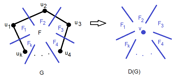
Figure 29: Matching between multi-angle and simple cycle for graph $D(G)$ (blue) and graph $G$ (black) in lemma 25.

Therefore, any multi-angle of the graph $G$ (the set of faces which contain correspondent vertex) matches bijectively with a face of the graph $D(G)$ and vice versa. Thus, for every vertex $D(D(v))=v$ and for every edge $e$ adjacent to this vertex $D(D(e))=e$. This can be continued for a whole graph and thus, $D(D(G))=G$. ∎

Corollary 8.

Any non-isomorphic connected graphs have non-isomorphic dual graphs.

Corollary 9.

$$\|V(D(G))\|=\|F(G)\|,\quad\|E(D(G))\|=\|E(G)\|,\quad\|F(D(G))\|=\|V(G)\|.$$

[1em]0em

Proof.

By definition: $\|V(D(G))\|=\|F(G)\|$. By lemma 24: $\|E(D(G))\|=\|E(G)\|$. Using the correspondence in lemma 25: $\|F(D(G))\|=\|V(G)\|$. ∎

Lemma 26.

Planar graph $G$ is Hamiltonian iff. there exist a representation and a simple cycle $C$ such that the parts of the dual graph $D(G)$ which belong to $int(C)$ and $out(C)$ are trees.

[1em]0em

Proof.

By the matching between vertices in the lemma 25 the existence of vertex of the graph $G$ that belongs to $int(C)$ or $out(C)$ is equivalent to the existence the cycle in the dual graph $D(G)$. ∎

Lemma 27.

The dual graph $D(G)$ is simple iff. $G$ is 3-edge connected.

[1em]0em

Proof.

The loop in the dual graph $D(G)$ corresponds to the edges of the graph $G$ which split the graph $G$ for two connected components after deleting these edges. Therefore, the absence of loops corresponded to 2-edge connectivity of the graph $G$. Multi-edges in $D(G)$ correspond to the adjacent faces, which have several common adjacent edges. Thus, the additional absence of multi-edges is corresponded to 3-edge connectivity of the graph $G$. ∎

Lemma 28.

A dual graph $D(G)$ has no loops, 2-connected and planar iff. the graph $G$ has no loops, simple 2-connected and planar.

[1em]0em

Proof.

Let’s proof sufficient condition. The necessary condition will hold by the lemma 25.

Assume the contrary: the dual graph has a vertex $v$ such that the graph $D(G)$ becomes not connected after deleting $u$. Consider two connected components $G_{1}$ and $G_{2}$ in $D(G)$. Let’s $M_{1}$ and $M_{2}$ be the maximal sub-graphs on vertices $V(G_{1})\bigcup\{v\}$ and $V(G_{2})\bigcup\{v\}$ respectively. Sub-graphs $M_{1}$ and $M_{2}$ should contain cycles $f_{1}$ and $f_{2}$ respectively, otherwise one of them is a tree and it holds a contradiction using the lemma 25 with no loops in $G$. Let’s denote the dual vertices corresponded to faces $f_{1}$ and $f_{2}$ by $u_{1}\in G$ and $u_{2}\in G$ (see figure 30). Let’s denote the vertex corresponded to outer face of $D(G)$ by $u$. Since any inner faces of $M_{1}$ has no adjacent edges with any inner face of $M_{2}$, any path from vertex $u_{1}$ to $u_{2}$ should contain $u$. This holds a contradiction with 2-connectivity of $G$. ∎

Lemma 29.

A dual graph $D(G)$ is simple, 3-connected and planar iff. the graph $G$ is simple 3-connected and planar.

[1em]0em

Proof.

The proof for this theorem is the same as for previous theorem, but in this case one should consider two faces: outer face that corresponds to the vertex $u\in G$ and “middle” face $f$ that corresponds to the vertex $w\in G$ (see figure 30). ∎

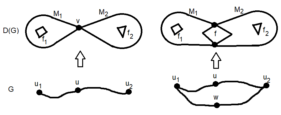
Figure 30: Graph $G$ and dual graph $D(G)$ for lemmas 28 (left) and 29 (right).

13.2 Steinitz theorem

Let’s start with several definitions and lemmas:

Definition 13.2.

Contraction of and edge $(u,v)$ is the operation that transform the graph $G$ to the graph $G^{\prime}$ by merging vertices $u$ and $v$ to a new vertex $w\in V(G^{\prime})$: $V(G^{\prime})=(V(G)\setminus\{u,v\})\bigcup\{w\}$ (see figure 31).

Definition 13.3.

Minor of a graph $G$ is a graph that is obtained from $G$ by contraction and deleting operations of edges.

Definition 13.4.

In series reduction is a contraction of an edge adjacent to the vertex of degree two. In parallel reduction is a deleting multiple edges between to vertices. SP-reduction of the graph $G$ is a sequence of series and parallel reductions obtained for the graph $G$ (see figure 31).

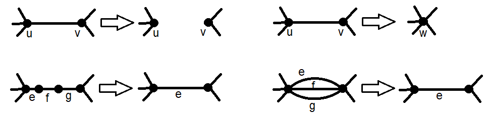
Figure 31: Deleting (left-top) and contraction (right-top) operations. In series (left-bottom) and parallel (right-bottom) reductions.

Definition 13.5.

Grid graph $G(k,l)$ is the graph on the plane with vertices coordinates $\{(a,b):0\leq a\leq k-1,0\leq b\leq l-1\}$ such that two vertices are connected if either their $x$-coordinates differ by 1 and $y$ coincide or $y$-coordinates differ by 1 and $x$ coincide.

Lemma 30.

Any planar graph is a minor of a grid graph.

[1em]0em

Proof.

Consider some representation of a planar graph $G$ on the plane $\mathbb{R}^{2}$. We can split any vertex such that $G$ will have a vertices of maximum degree 4 (see figure 32). Let’s $U_{r}(v)$ be a disk in $\mathbb{R}^{2}$ with center in $v$ and radius $r$, $\partial U_{r}(v)$ be the boundary of the disk and $U_{r}(e)=\bigcup\limits_{p\in e}U_{r}(p)$.

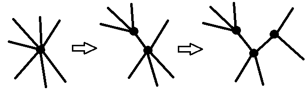
Figure 32: Splitting in small neighbourhood of vertex with degree more than 4 to vertices which has maximum degree 4 for lemma 30.

Let’s find $\epsilon_{1},\epsilon_{2}$ and $\epsilon_{3}$ such that:

1. Consider for every vertex $v_{j}$ a point $v^{\prime}_{j}\in U_{\epsilon_{3}}(v_{j})$ with rational coordinates. For any $j$: $U_{\epsilon_{3}}(v_{j})\subset U_{\epsilon_{1}}(v^{\prime}_{j})$.

2. For any $j$ the number of intersections of $\partial U_{\epsilon_{1}}(v^{\prime}_{j})$ and an edge $e$ should be equal to 1 for $e$ adjacent to $v_{j}$ and 0 otherwise.

3. For any edge $e$ all regions $U_{\epsilon_{2}}(e)\setminus(\bigcup\limits_{j=1}^{n}U_{\epsilon_{1}}(v^{\prime}_{j}))$ are connected and disjoint.

Since $U_{\epsilon_{3}}(v_{j})\subset U_{\epsilon_{1}}(v^{\prime}_{j})$ thus $v_{j}\in U_{\epsilon_{1}}(v^{\prime}_{j})$. Let’s denote by $e_{i,j}$ the intersections of edges $e_{i}$ and $\partial U_{\epsilon_{1}}(v^{\prime}_{j})$. Consider the points with rational coordinates $p_{i,j}\in\partial U_{\epsilon_{1}}(v^{\prime}_{j})$ such that $p_{i,j}\in U_{\epsilon_{2}}(e_{i,j})$. Since all vertices have the maximum degree 4, any $\partial U_{\epsilon_{1}}(v^{\prime}_{j})$ can contain maximum 4 different points $p_{i,j}$.

Let’s scale the coordinates of $\mathbb{R}^{2}$ by multiplication of the product of denominators of all corresponding points. Thus all corresponded points will have integer coordinates. For any region corresponded to $U_{\epsilon_{1}}(v^{\prime}_{j})$ there exists the natural number $C_{j}$ for scaling coordinates of $\mathbb{R}^{2}$ such that after scaling there exist less or equal four vertex independent paths from $v^{\prime}_{j}$ to $p_{i,j}\in\partial U_{\epsilon_{1}}(v^{\prime}_{j})$ with consequent vertices in $U_{\epsilon_{1}}(v^{\prime}_{j})$ with either their $x$-coordinates differ by 1 and $y$ coincide or $y$-coordinates differ by 1 and $x$ coincide. There exist natural numbers $D_{i}$ with the same properties for any region $U_{\epsilon_{2}}(e_{i})\setminus(\bigcup\limits_{j=1}^{n}U_{\epsilon_{1}}(v^{\prime}_{j}))$ and two vertices $p_{i,j}$ and $p_{i,k}$ corresponded to the edge $e_{i}$. By scaling, finally for the product of all $C_{j}$ and $D_{i}$ and shifting coordinates one can obtain required grid graph. ∎

Definition 13.6.

$\Delta Y$ operation is an operation replacing a triangle that bounds a face by 3-star that connects the same vertices or vice versa (see figure 33). If a triangle transforms to 3-star it is called $\Delta$-to-$Y$ operation and the reverse is called $Y$-to-$\Delta$ operation.

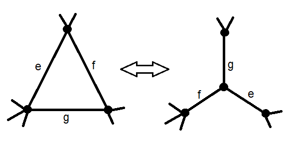
Figure 33: $\Delta Y$ operation.

Because $\Delta Y$ operations can cause multi-edges in new graph in this subsection all graphs can be considered as not simple.

Lemma 31.

1. Let $v\in G$ is a vertex of degree 3 that has three non-parallel adjacent edges $(e,f,g)$.

2. If $G$ has no loops, planar and 2-connected, then the result of $Y$-to-$\Delta$ operation and then series of $SP$-reductions also has no loops, planar and 2-connected.

3. Let $G$ be simple, planar, 3-connected graph and not $K_{4}$, then the result of $Y$-to-$\Delta$ operation and then series of $SP$-reductions is also simple, planar, 3-connected.

[1em]0em

Proof.

By Mengers theorem 25 there exist 2 or 3 vertex independent paths between any two vertices in $G$. Paths which don’t contain vertex $v$ after $Y$-to-$\Delta$ operation will not change. There can be only one path from the independent set that contains vertex $v$ and thus edges $e$ and $f$ without loss of generality. After $Y$-to-$\Delta$ operation this path will walk through the new edge $g$. ∎

Lemma 32.

1. Let $(e,f,g)$ be three non-parallel edges which form a triangle.

2. If $G$ has no loops, planar and 2-connected, then the result of $\Delta$-to-$Y$ operation and then series of $SP$-reductions is also has no loops, planar and 2-connected.

3. Let $G$ be simple, planar 3-connected graph, then the result of $\Delta$-to-$Y$ operation and then series of $SP$-reductions is also simple, planar and 3-connected.

[1em]0em

Proof.

Let’s note that $Y$-to-$\Delta$ operation for a graph $G$ corresponds to $\Delta$-to-$Y$ for the dual graph $D(G)$ and vice versa. Also in series reduction for the graph $G$ corresponds to in parallel reduction for the dual graph $D(G)$ and vice versa. The multi edges corresponds to the object in dual graph that can be reduced by in series reduction to just one edge. By using this facts and lemmas 28 and 29 this lemma is led to the previous one. ∎

Definition 13.7.

A 2-connected graph $G$ is $\Delta Y$ reducible to the graph $G^{\prime}$ if it can be transformed to the graph $G^{\prime}$ by sequence of $\Delta Y$ operations and $SP$-reductions.

Lemma 33.

Any grid graph $G(k,l):k,l\geq 3$ is $\Delta Y$ reducible to the graph $K_{4}$.

[1em]0em

Proof.

Let’s use two following operations (figure 34) in the grid graph $G(k,l)$.

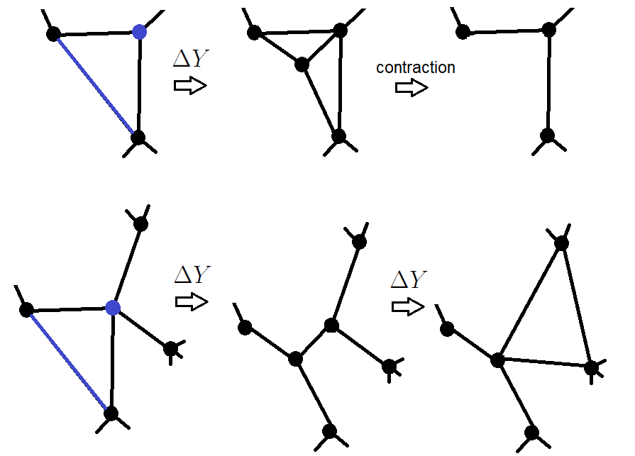
Figure 34: Two operations in lemma 33: operation 1 for triangle with adjacent vertex with degree 3 (top) and operation 2 for triangle with adjacent vertex with degree 4 (bottom).

First, let’s use in series reduction to transform the left-bottom and right-top squares to triangles. Then, transfer the left-bottom triangle to the top row by series of operation 2. If by this the multi-edges are obtained, use in parallel reduction, if it is not, use operation 1 to delete transferred triangle. Use this procedure for second square in the bottom row. By this procedure one can delete all squares of the bottom row. The symmetrical procedure can be used for deleting columns from left to right. Therefore, this grid graph can be reduced to the grid graph $G(2,2)$. See figure 35 to obtain the graph $K_{4}$ from $G(2,2)$.

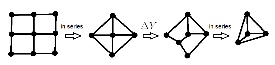
Figure 35: The series of reductions to obtain the graph $K_{4}$ from $G(2,2)$ for lemma 33.

∎

Let’s $C_{2}$ be a graph with two vertices and two multi-edges between them.

Lemma 34.

If a planar graph with no loops $G$ is $\Delta Y$ reducible to the graph $C_{2}$, then so is for every 2-connected minor without loops of $G$.

[1em]0em

Proof.

Let’s proof it by induction for the number of $\Delta Y$ reductions necessary to obtain the graph $C_{2}$:

The base: any 2-connected minor of $C_{2}$ is $C_{2}$.

Now, let for every $G$ that can be $\Delta Y$ reduced to the graph $C_{2}$ by $k$ steps, every 2-connected minor is also $\Delta Y$ reducible to $C_{2}$. Let’s prove it for $G$ that can be $\Delta Y$ reduced to the graph $C_{2}$ by $k+1$ steps. Consider the graph $G^{\prime}$ after one step of $\Delta Y$ reduction. Let’s $H$ be a 2-connected minor without loops of $G$.

1. If $H$ doesn’t contain the part that is changed by current $\Delta Y$ reduction from $G$ to $G^{\prime}$ then $H$ is 2-connected minor of $G^{\prime}$. Therefore $H$ is $\Delta Y$ reducible to $C_{2}$ by the inductive assumption.

2. If $H$ contains whole part that is changed by current $\Delta Y$ reduction from $G$ to $G^{\prime}$ then this reduction can be used in $H$ to obtain the graph $H^{\prime}$. By the lemmas 31 and 32 $H^{\prime}$ will be 2-connected minor without loops of $G^{\prime}$. Therefore, $H^{\prime}$ and hence $H$ are $\Delta Y$ reducible to $C_{2}$.

3. If $H$ doesn’t contain whole part then the current reduction is $\Delta$-to-$Y$ or $Y$-to-$\Delta$. Let’s denote the corresponding edges by $(e,f,g)$, and $e$ or $e,f$ will be the part of the graph $H$ without loss of generality. Let’s consider cases:

   1. The current reduction is $\Delta$-to-$Y$.

      1. If $H$ can be obtained from $G$ by one contraction of the edge $g$ then $H$ will be the minor of $G^{\prime}$ by contraction of corresponded edges $e,f$ in $G^{\prime}$.

      2. If $H$ can be obtained from $G$ by contraction of two edges or more, then $H$ will contain a loop. This holds a contradiction.

      3. If $H$ can be obtained from $G$ by one deletion of the edge $g$ then $H$ will be the minor of $G^{\prime}$ by contraction the corresponded edge $g$ in $G^{\prime}$.

      4. If $H$ can be obtained from $G$ by deletion of the edges $f,g$ then $H$ will be the minor of $G^{\prime}$ by the deletion of the corresponded edge $e$ and contraction the corresponded edge $f$ or $g$ in $G^{\prime}$.

   2. The current reduction is $Y$-to-$\Delta$.

      1. If $H$ can be obtained from $G$ by contraction of any edges then $H$ will contain a loop. This holds a contradiction.

      2. If $H$ can be obtained from $G$ by deletion of one edge $g$ then let’s $H^{\prime}$ be the graph that is obtained by $H$ by in series reduction of the part $\{e,f\}$. Since $H^{\prime}$ is a minor of $G^{\prime}$ then $H^{\prime}$ and hence $H$ are $\Delta Y$ reducible to $C_{2}$.

      3. If $H$ can be obtained from $G$ by deletion of two or more edges then $H$ will be not 2-connected. This holds a contradiction.

∎

Corollary 10.

Any simple 3-connected planar graph $G$ is $\Delta Y$ reducible to the graph $K_{4}$.

[1em]0em

Proof.

By the lemma 30 $G$ is a minor of a grid graph $G(k,l)$. This grid graph $G(k,l)$ is $\Delta Y$ reducible to the graph $K_{4}$ by the lemma 33. Let’s note that $K_{4}$ is also $\Delta Y$ reducible to $C_{2}$. Hence, $G$ is $\Delta Y$ reducible to $C_{2}$ by the lemma 34. Let’s prove that $G$ is $\Delta Y$ reducible to $K_{4}$ by the induction of the number edges in $G$:

1. A simple 3-connected planar graph with the smallest number of edges in $K_{4}$ by the lemma 11 for $(k,l,d)$ graphs.

2. Let’s any simple 3-connected planar graph $G$ with $k$ edges is $\Delta Y$ reducible to $K_{4}$. Let’s prove it for $G$ with $k+1$ edges. Consider the $\Delta Y$ reduction of $G$ to $C_{2}$. Since $C_{2}$ has only two edges then there will be step with $SP$-reduction in $\Delta Y$ sequence. Let’s $G^{\prime}$ be the graph that is obtained from $G$ after the first $SP$-reduction. By the lemma 29 $G^{\prime}$ is simple, planar, 3-connected and has less edges than $G$. Then $G^{\prime}$ and hence $G$ are $\Delta Y$ reducible to $K_{4}$ by the inductive assumption.

∎

Theorem 20 (Steinitz).

A simple connected graph is planar and 3-connected iff. it is a graph of a convex polyhedron.

[1em]0em

Proof.

1. Necessarity. Let’s proof the following: let $G^{\prime}$ is a graph that obtained from $G$ by one $\Delta Y$ operation and $SP$-reduction and $G^{\prime}$ is a graph of a convex polyhedron $P(G^{\prime})$ then $G$ is also a graph of a convex polyhedron $P(G)$. Let’s consider cases:

   1. If the current $\Delta Y$ operation is $\Delta$-to-$Y$ operation then the polyhedron $P(G)$ can be obtained from the polyhedron $P(G^{\prime})$ by section of the plane $\pi$ (see figure 36).

      

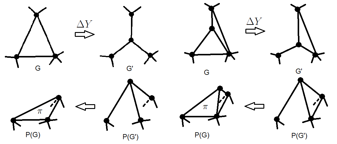
      Figure 36: $\Delta$-to-$Y$ operation without $SP$-reduction (left-top) and corresponded section of the polyhedron $P(G^{\prime})$ by the plane $\pi$ (left-bottom). $\Delta$-to-$Y$ operation with $SP$-reduction (in series, right-top) and corresponded section of the polyhedron $P(G^{\prime})$ by the plane $\pi$ (right-bottom).

   2. If the current $\Delta Y$ operation is $Y$-to-$\Delta$ operation. Consider the corresponded triangle $T\in P(G^{\prime})$. This triangle is adjacent to three faces $F_{1},F_{2},F_{3}$. Faces $F_{1},F_{2}$ and $F_{3}$ don’t intersect in one point because otherwise the polyhedron $P(G^{\prime})$ is tetrahedron and thus $G^{\prime}$ is $K_{4}$, that implies that $G$ is not 3-connected. Then, do the reverse operation like in figure 36 left, but with some deformation: compress the triangle in the face $T$ and deform $P(G^{\prime})$ such that planes corresponded to $F_{1},F_{2}$ and $F_{3}$ become intersected in one point (see figure 37) and extend current faces to this intersection. Obtained polyhedron will be convex and correspond to the graph $G$.

      

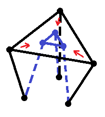
      Figure 37: Deformation of the polyhedron $P(G^{\prime})$ corresponded to the case 1b of the Steinitz theorem.

   Let’s note that in each case all transformations which have been done preserve convexity of the polyhedron.

2. Sufficiency. In the Euler theorem 10 the planarity property is proved. Let’s prove by deletion of any two vertices $u,v$ the graph $G$ remains connected.

   1. Consider the case when $u,v\in\pi$. Let’s prove that for any two vertices $\notin\pi$ there exists path between them that doesn’t intersect the face $\pi$. Consider the path $P$ between any two vertices in $G$. Let’s transform this path by following:

      1. Consider the case when $P$ contains an edge $e\in\pi$. Let’s denote the another adjacent face (not $\pi$) by $F$. Transform the path $P$ to $(P\setminus e)\bigcup(F\setminus e)$. Since faces $F$ and $\pi$ can intersects only by one edge (property 2 of polyhedrons), the number of edges in path $P$ which belongs to $\pi$ will decreased by 1. Do this for every edge in $P\bigcap\pi$.

      2. If $P$ contains a vertex $v\in\pi$. Consider the polyhedral angle corresponded to vertex $v$ (or all faces which contain $v$). Let’s denote the adjacent to $v$ edges in $P$ by $e_{1}$ and $e_{n}$. For the edge $e_{1}$ there exists a face $F_{1}\neq\pi$ that contains $e_{1}$. Let’s do the transformation like in case 2(a)i for the edge $e_{1}$. By this transformation the edge $e_{1}$ transforms to the path through the face $F_{1}$. Let’s denote the new edge of $F_{1}$ adjacent to the vertex $v$ by $e_{2}$ and continue this procedure for $e_{2}$ and so on. In the end transform the path $P$ to $(P\setminus\{e_{n-1},e_{n}\})\bigcup(F_{n-1}\setminus\{e_{n-1},e_{n}\})$.

      By this transformations one can modify the path between any two vertices $\notin\pi$ by a path that doesn’t intersect the face $\pi$. Therefore, there exists path between any two vertices in $G\setminus\{u,v\}$.

   2. Vertices $u,v$ don’t belong to the same face. Consider the path between any two vertices that contains the vertex $u$ without loss of generality. Transform the path using procedure in the case 2(a)ii. Since vertices $u,v$ don’t belong to the same face, the faces $F_{1},F_{2},...,F_{n-1}$ don’t contain the vertex $v$ and hence, the new transformed path doesn’t contain the vertices $u$ and $v$. Therefore, there exists path between any two vertices that doesn’t contain the vertices $u$ and $v$.

∎

13.3 Dual polyhedrons

Definition 13.8.

Dual polyhedron $D(P)$ for a convex polyhedron $P$ is defined by following:

1. Consider the 3-dimensional coordinates of vertices of polyhedron $P$. Each face $v_{1}v_{2}...v_{k}\in P$ match with the vertex $u=\frac{1}{k}\sum_{i=1}^{k}v_{i}.$

2. If any two faces of $P$ are adjacent then add an edge in the dual graph $D(P)$ between two vertices which are matched to these faces.

NB! A dual polyhedron is constructed unique by this matching.

NB! The graph of dual polyhedron $D(P)$ is dual to the graph of a polyhedron $P$.

Lemma 35.

$int(D(P))\subset int(P)$.

[1em]0em

Proof.

Use the convex property in following:

$$\forall u,v\in D(P)\Rightarrow u,v\in\partial P\Rightarrow(u,v)\subset int(P)\Rightarrow D(P)\subset P\Rightarrow int(D(P))\subset int(P).$$

∎

Lemma 36.

The dual polyhedron is convex.

[1em]0em

Proof.

Since the graph of dual polyhedron $D(P)$ is dual to the graph of a polyhedron $P$, then in the same way like in lemma 25 this matching can be continued to the matching between faces and multi-angles of the polyhedron $P$ and the dual polyhedron $D(P)$ such that there is correspondence between the edges of a face and a multi-angle and the vertices of the face are corresponded to the faces of the multi-angle (see figure 38).

Now let’s assume the contrary: there exist two faces $F_{1},F_{2}\in D(P)$ such that the edge $(u,v):u\in F_{1},v\in int(D(P))$ intersect the face $F_{2}$. The vertex $v\in int(P)$ by lemma 35. By the correspondence below there are a multi-angles at vertices $h_{1}$ and $h_{2}$ which match to the faces $F_{1}$ and $F_{2}$ (see figure 38). Hence, the edge $(u,v)$ such that $u\in P$ and $v\in int(P)$ intersects with the polyhedron $P$. This holds a contradiction. ∎

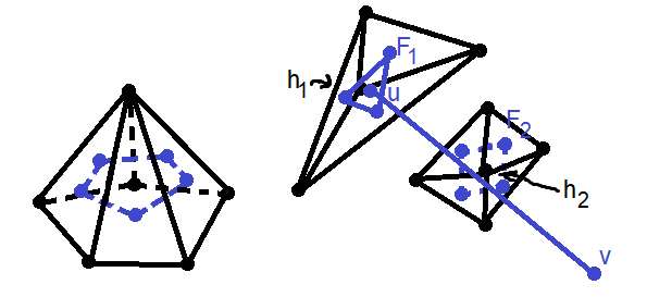
Figure 38: For the lemma 36: correspondence between a face of dual polyhedron $D(P)$ (blue, left) and a multi-angel of polyhedron $P$ (black, left). Two faces $F_{1}$ and $F_{2}$, the edge $(u,v)$ of dual polyhedron $D(P)$ (blue, right) and corresponded multi-angels at vertices $h_{1}$ and $h_{2}$.

Consider the duality relationship for platonic solids (see figure 39):

1. Tetrahedron $\rightarrow$ Tetrahedron

2. Octahedron $\rightarrow$ Cube

3. Icosahedron $\rightarrow$ Dodecahedron

4. Cube $\rightarrow$ Octahedron

5. Dodecahedron $\rightarrow$ Icosahedron

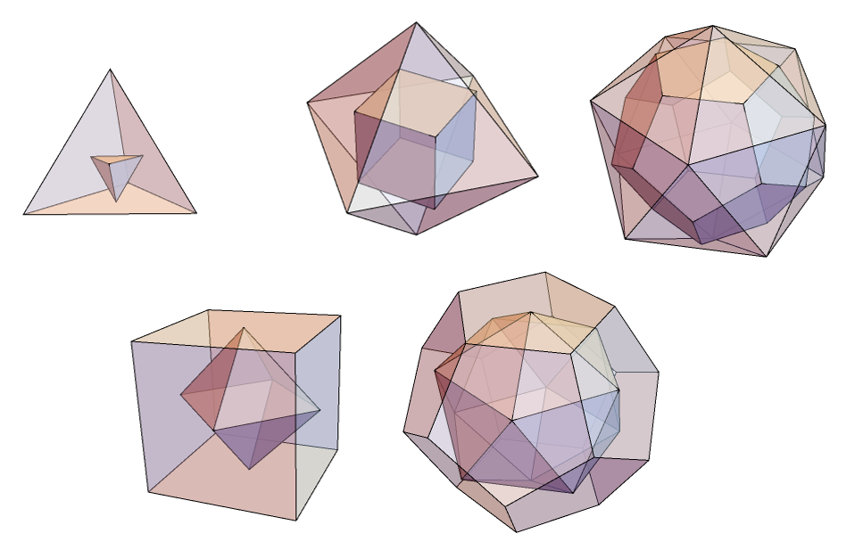
Figure 39: Dual polyhedrons for platonic solids.

Theorem 21 (Whitney).

Any planar 3-connected graph has unique dual graph up to isomorphism.

[1em]0em

Proof.

Let’s assume the contrary: a planar 3-connected graph $G$ has two non-isomorphic dual graphs $D_{1}$ and $D_{2}$. By the Steinitz theorem 20 any 3-connected graph $G$ is a graph of a convex polyhedron $P(G)$. Any dual graph $D(G)$ is also 3-connected by the lemma 29 thus it is also a graph of convex polyhedron $P(D(G))$. Since $D_{1}$ and $D_{2}$ are not isomorphic the graphs of two polyhedrons $P(D_{1})$ and $P(D_{2})$ are not isomorphic. By the lemma 25 graphs of dual polyhedrons $D(P(D_{1}))$ and $D(P(D_{2}))$ are isomorphic to the graph $G$ and thus isomorphic. Let’s denote this isomorphism by $i_{1}:D(P(D_{1}))\rightarrow D(P(D_{2}))$. By matching in the lemma 25 this isomorphism defines isomorphism of their duals: $i^{\prime}_{1}:D^{2}(P(D_{1}))\rightarrow D^{2}(P(D_{2}))$. Dual polyhedron $D^{2}(P(D_{1}))$ is isomorphic to $P(D_{1})$ and $D^{2}(P(D_{2}))$ is isomorphic to $P(D_{2})$ then there exist $i_{2}:D^{2}(P(D_{1}))\rightarrow P(D_{1})$ and $i_{3}:D^{2}(P(D_{2}))\rightarrow P(D_{2})$. The composition $i_{3}\circ i^{\prime}_{1}\circ i_{2}^{-1}:P(D_{1})\rightarrow P(D_{2})$ and thus they are isomorphic. ∎

13.4 Algorithms

Dual graph constructing algorithm.

This algorithm constructed the dual graph $D(G)$ corresponding to a planar representation of a connected graph $G$.

Description:

1. Initialize 2-dimensional array $a=[a_{1}[v],a_{2}[v]]$ corresponded to edges of a dual graph $D(G)$ with dimensions $2\times\|E(G)\|$.

2. Find all bridges using any bridge-detecting algorithm.

3. For any 2-edge connected component $G$ choose an edge $e\in G$ and use any algorithm of searching shortest path $P$ in $G\setminus e$ between two vertices adjacent to the edge $e$ to find a simple cycle $C=P\bigcup e$ in $G$.

4. For every edge $e_{j}\in C$ add vertex $v_{1}$ in $a_{1}[j]$.

5. Choose another edge $e\in G$ and use any algorithm of searching shortest path $P_{1}$ in $G\setminus e$ between two vertices adjacent to the edge $e$ to find a simple cycle $C=P_{1}\bigcup e$ in $G$.

6. Check that this cycle is new cycle by checking whether all $a[j]$ corresponded to the edges of $C$ don’t contain the same vertex. If it is the same cycle (all $a[j]$ contain the same vertex) find another shortest path $P_{2}$ (by deleting one of adjacent edges to $e$ in $P_{1}$) in $G\setminus e$. And let $C=P_{2}\bigcup e$.

7. For every edge $e_{j}\in C$ add vertex $v_{2}$ either in $a_{1}[j]$ or in $a_{2}[j]$ if $a_{1}[j]$ is not empty.

8. Do 5-7 for every another edge in $G$.

9. For each empty $a_{2}[j]$ add a vertex $v_{0}$ that corresponds to the outer face of the graph.

10. For every not assigned bridge $b$ find the path $P$ from this bridge to a vertex that contains an edge $e_{i}$ with not empty $a_{2}[i]$. For every bridge $e_{j}\in P\bigcup{b}$ add in $a_{1}[j]$ and $a_{2}[j]$ the value $a_{2}[i]$.

NB! The complexity of this algorithm using breadth first search or depth first search for connected graphs equals to $\mathbf{O(\|E\|^{2})}$.

Definition 13.9.

The dual graph $D(G)$ is called simple* iff. it is simple after the deletion of vertex corresponded to the outer face of $G$.

Consider the algorithm corresponded to simple* dual graphs:

Lee algorithm.

This algorithm finds the shortest path through inner faces between any two inner faces of a planar representation of a graph with simple* dual graph.

Description:

1. Construct the dual graph $D(G)$ for the current graph $G$ and delete the vertex corresponded to outer face of the current graph $G$.

2. Mark the vertices corresponded to the same depth (or distance from starting point) corresponded to breadth first search by this depth.

3. Algorithm terminates when the end point is marked.

To find the shortest path walk through the vertices corresponded to reverse order of marked numbers (from ending point to starting, see figure 40).

NB! The complexity of this algorithm (without constructing dual graph) equals to the complexity of breadth first search for connected graphs $\mathbf{O(\|E\|)}$.

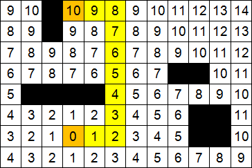
Figure 40: Result of the Lee algorithm.

Modifications of Lee algorithm:

1. In this algorithm any constructing shortest path algorithm can be used. The complexity will be equal to the complexity of corresponded algorithm.

2. One can consider different time travelling from one face to another in the planar representation. Thus, the additional weights can be added in the dual graph. And in this case the shortest path algorithms for weighted graphs can be used.

3. One can apply the breadth first search to starting point and ending point in parallel. Then these two algorithms intersect by a vertex the shortest path can be constructed.

4. If there is some information of the dual graph or path, for example, it is known that the path should contain some vertex. Lee algorithm can be applied to this vertex or done parallel from starting vertex, ending vertex and the current vertex like in 3.

14 Flows on graphs

14.1 Decomposition of flows

Definition 14.1.

A flow network is directed graph $G$ with positive weights $w(u,v)$ with two highlighted vertices $s$ (source) and $t$ (terminal) and capacity function $c:V(G)\times V(G)\rightarrow\mathbb{R}^{+}$ defined by following:

$$c(u,v)=\begin{cases}w(u,v)&(u,v)\in E(G)\\ 0&\text{otherwise}\end{cases}.$$

Let’s consider a flow network $G$.

Definition 14.2.

A flow is a function $f:V(G)\times V(G)\rightarrow\mathbb{R}$ satisfied the following properties:

1. $f(u,v)=-f(v,u)$ (skew symmetry),

2. $f(u,v)\leq c(u,v)$ (capacity constraint),

3. $\forall u\in V(G)\setminus\{s,t\}:\sum\limits_{v\in V(G)}f(u,v)=0$ (conservation of a flow).

A flow $f$ value is $F=\sum\limits_{v\in V(G)}f(s,v)$.

NB! By skew symmetry a value of the flow $F$ can be less than 0.

Statement 3 (Sum of flows).

Consider a flow network $G$ with two flows: $f_{1}$ and $f_{2}$. If $f_{1}(u,v)+f_{2}(u,v)\leq c(u,v)$ for any edge $(u,v)$ then $f_{1}+f_{2}$ also a flow and $F(f_{1}+f_{2})=F_{1}+F_{2}$.

[1em]0em

Proof.

It easy holds from definition. ∎

Theorem 22 (Decomposition of flow).

For a positive flow $f:F>0$ there exist at most $\|E\|$ simple paths $P_{i}$ from $s$ to $t$ and simple cycles $C_{i}$ such that

$$f=\sum\limits_{i}f_{P_{i}}+\sum\limits_{i}f_{C_{i}}\text{ and }F=\sum\limits_{i}f(P_{i}),$$

where $f(P)=\min_{e\in P,\ f(e)>0}f(e)$ and

$$f_{P}(u,v)=\begin{cases}f(P)&(u,v)\in P\\ -f(P)&(v,u)\in P\\ 0&\text{otherwise}\end{cases}.$$

[1em]0em

Proof.

Since the flow $f$ is positive then there exists an edge $(s,v_{1})$ with positive flow $f(s,v_{1})$. By the skew symmetry $f(v_{1},s)=-f(s,v_{1})$ and thus by conservation of a flow there exists an edge $(v_{1},v_{2})$ with positive flow $f(v_{1},v_{2})$. If these procedure reaches $t$ then denote this path by $P_{1}$. If these procedure reaches some visited vertex then denote this corresponded simple cycle by $C_{1}$. Let’s denote this cycle or path by $P$.

Consider a flow $f^{\prime}(u,v)=\begin{cases}f(P)&(u,v)\in P\\ -f(P)&(v,u)\in P\\ 0&\text{otherwise}\end{cases}.$

By decreasing our flow $f$ by this flow $f^{\prime}$ new flow becomes 0 at at least one edge. Then all edges from the source $s$ will be with 0 flow. One can obtain this procedure starting with all the rest vertices with positive adjacent edges. Thus by doing the same procedure at most $\|E\|$ times one can obtain the decomposition. ∎

This theorem simple implies the decomposition algorithm.

NB! Since the number of steps for constructing a cycle or a path in the theorem 22 less or equal the number of vertices in the graph and the number of such cycles and paths is $O(\|E\|)$ thus the complexity of decomposition algorithm is $\mathbf{O(\|V\|\|E\|)}$.

Definition 14.3.

A residual network $G_{f}=(V(G),E_{f})$ is a flow network with edges $E_{f}$ with non-negative residual capacity $c_{f}(u,v)=c(u,v)-f(u,v)$.

Lemma 37 (Two flows).

Let $f$ and $h$ be two flows in a flow network $G$ then $h$ can be represented as a sum $f+f^{\prime}$, where $f^{\prime}$ is a flow in the residual network $G_{f}$ with the value $F^{\prime}=H-F$.

[1em]0em

Proof.

It easy holds from definition. ∎

Lemma 38 (Subtraction of flows).

Let $f$ and $g$ be flows with equal values in a flow network $G$. Then $g=f+\sum\limits_{i}f_{C_{i}},$ where $f_{C_{i}}$ are flows in the residual network $G_{f}$ among a cycles $C_{i}$.

[1em]0em

Proof.

By the previous lemma there exists a flow $f^{\prime}$ in $G_{f}$ such that $g=f+f^{\prime}$. Since $F^{\prime}=G-F=0$ thus decomposition algorithm will obtain only cycles $C_{i}$ in the residual network $G_{f}$. ∎

Definition 14.4.

$s,t$-cut $(A,B)$ is a distribution of the vertex set $V(G)$ by two parts $A,B$ such that:

1. $A\bigcup B=V(G)$,

2. $A\bigcap B=$ Ø,

3. $s\in A,\ t\in B$.

Definition 14.5.

A capacity of the $s,t$-cut $(A,B)$ is

$$C(A,B)=\sum\limits_{u\in A}\sum\limits_{v\in B}c(u,v).$$

Definition 14.6.

A flow through the $s,t$-cut $(A,B)$ is

$$F(A,B)=\sum\limits_{u\in A}\sum\limits_{v\in B}f(u,v).$$

Lemma 39 ($s,t$-cut flow).

A flow through any $s,t$-cut is equal to the flow value.

[1em]0em

Proof.

By the skew symmetry: $\sum\limits_{u\in A}\sum\limits_{v\in A}f(u,v)=0$.

$$\sum\limits_{u\in A}\sum\limits_{v\in B}f(u,v)=\sum\limits_{u\in A}\sum\limits_{v\in B}f(u,v)+\sum\limits_{u\in A}\sum\limits_{v\in A}f(u,v)=\sum\limits_{u\in A}\sum\limits_{v\in V(G)}f(u,v)=$$

$$=\sum\limits_{v\in V(G)}f(s,v)+\sum\limits_{u\in A\setminus\{s\}}\sum\limits_{v\in V(G)}f(u,v)\overset{\text{conservation low}}{=}F.$$

∎

Corollary 11.

The sum of flows from the source is equal to the sum of flows to the terminal.

14.2 Max-flow

Definition 14.7.

The max-flow is a flow with maximal value in a flow network $G$.

NB! The value of the max-flow should be non-negative.

Lemma 40 (Necessary and sufficient condition of positive max-flow value).

The max-flow value is positive iff. there exists a path from the source to the terminal.

[1em]0em

Proof.

1. Sufficiency. Let $c_{P}$ be the minimal capacity value among the path $P$.
   Let’s define a flow: $f(u,v)=\begin{cases}c_{P}&(u,v)\in P\\ -c_{P}&(v,u)\in P\\ 0&otherwise\end{cases}.$
   The flow value $F=c_{P}>0$ thus the max-flow value is positive.

2. Necessarity. Let’s assume the contrary: there is no path from the source to the terminal. Let’s denote by $A$ a set of vertices which are reachable from the source and $B$ will be all the rest. Thus $c(A,B)=0$ and by $s,t$-cut flow lemma 39:

   $$0<F=F(A,B)\leq c(A,B)=0$$

   holds contradiction.

∎

NB! In the case of max-flow, flow value is positive is equivalent to flow value is not zero.

Lemma 41 (Of a path in residual network).

A flow $f$ is max-flow iff. there is no path from the source to the terminal in the residual network $G_{f}$.

[1em]0em

Proof.

1. Necessarity. Let $f$ be the max-flow. Assume the contrary: there exists a path $P$ from the source to the terminal in the residual network $G_{f}$. Let $c_{f,P}$ be the minimal capacity value in $G_{f}$ among the path $P$. Let’s define a flow:

   $$f^{\prime}(u,v)=\begin{cases}c_{f,P}&(u,v)\in P\\ -c_{f,P}&(v,u)\in P\\ 0&otherwise\end{cases}.$$

   The flow value $F^{\prime}=c_{f,P}$. Since $f(u,v)+f^{\prime}(u,v)\leq f(u,v)+c_{f}=c(u,v)$ then $f+f^{\prime}$ is a flow and $F+F^{\prime}>F$. This holds a contradiction with max-flow.

2. Sufficiency. Assume the contrary: there exists max-flow $f^{\prime}\neq f$. By the two flows lemma 37 the flow $f^{\prime}-f$ is a flow in residual network $G_{f}$ with the flow value $F^{\prime}-F>0$ thus the maximal flow on $G_{f}$ is positive and thus be the lemma 40 there exists a path in $(G_{f})_{f^{\prime}-f}=G_{f^{\prime}}$. This holds the contradiction by necessarity condition.

∎

Definition 14.8.

Min-cut is a $s,t$-cut $(A,B)$ with the minimal capacity $(A,B)$.

Theorem 23 (Ford–Fulkerson).

The max-flow value equals to the min-cut capacity value.

[1em]0em

Proof.

Let $f$ be the max-flow and $(A_{min},B_{min})$ be the min-cut. By the $s,t$-cut lemma 39: $F=F(A_{min},B_{min})\leq c(A_{min},B_{min})$.

By the lemma of path in residual network 41 there is no paths between the source $s$ and terminal $t$ in the residual network $G_{f}$. Let’s denote by $A$ the subset of vertices in $G_{f}$ which are reachable from $s$ and by $B$ all the rest.

$$0=c_{f}(A,B)=c(A,B)-f(A,B)\implies F=f(A,B)=c(A,B)\geq c(A_{min},B_{min})\implies$$

$$\implies F=c(A_{min},B_{min}).$$

∎

Consider algorithms for constructing max-flow:

1. Ford–Fulkerson algorithm.
   This algorithm finds max-flow in a flow network $G$ from the source $s$ to the terminal $t$.
   Description:

   1. Initialize max-flow $f_{max}=0$.

   2. Find any path $P$ from $s$ to $t$ in $G$.

   3. Find the minimum capacity $c_{p}$ among this path $P$.

   4. Construct the flow $f$ with $c_{p}$ among the path and 0 otherwise (see lemma 40).

   5. Add new flow $f$ to the max-flow $f_{max}$. Do steps 1b- 1d for residual network $G_{f_{max}}$ and find a new flow $f$.

   NB! The complexity of this algorithm corresponds to the weights of a network.

   NB! In some special cases this algorithm may work very slow (see ex 14.1) and moreover not terminate.

   Example 14.1.

   Let’s consider several steps of Ford–Fulkerson algorithm:

   

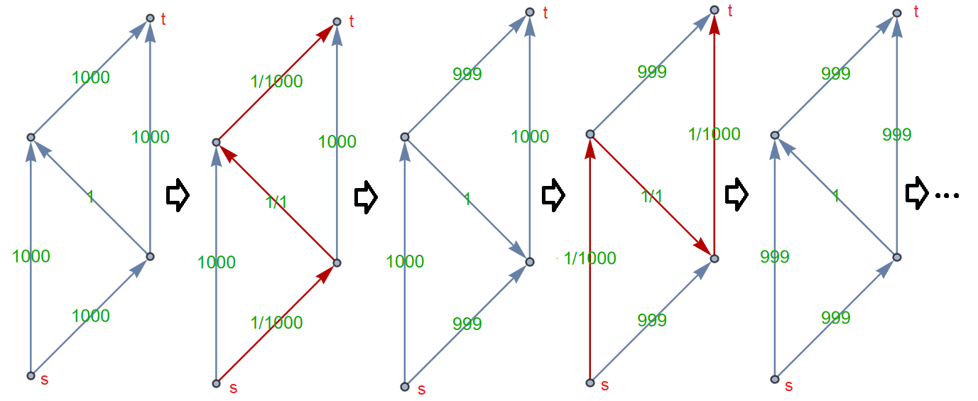
   Figure 41: Steps of Ford–Fulkerson algorithm. First: the flow network $G$. Second: the flow $f$ versus capacity among the path (red). Third: the residual network $G_{f}$ and so on.

   Since the path construction algorithm is not specified the path can be chosen like in this figure and thus this algorithm will do about 2000 cycles. It is easy to see that one can change the paths such that it will terminate by 2 steps.

   The next algorithm solves this problem:

2. Edmonds–Karp algorithm.
   This algorithm finds max-flow in a flow network $G$ from the source $s$ to the terminal $t$.
   Description:
   This algorithm works the same as Ford–Fulkerson algorithm but at the step 1b BFS algorithm is being used for searching the path with the minimum number of edges.

   NB! The complexity of this algorithm corresponds to the weights of a network and also may work very slow.

3. Dinic algorithm.

   To explain next algorithm let’s first give some definitions:

   Definition 14.9.

   A level graph corresponded to the root $s$ of a directed unweight graph $G$ is a sub-graph $G_{L}=(V(G),E_{L})$ such that $(u,v)\in E_{L}\subset E(G)\iff dist(s,v)=dist(s,u)+1$.

   NB! A level graph can be easily constructed using BFS algorithm starting from the root $s$. Note that $BFS(v)=dist(s,v),\ \forall v\in V(G)$.

   Definition 14.10.

   A block flow is the max-flow in the level graph $G_{L}$ corresponded to the source $s$.

   Statement 4.

   A level graph is acyclic graph and all paths from the root $s$ to any vertex $v$ have the same length.

   [1em]0em

   Proof.

   Easily holds from definition. ∎

   Now let’s consider the Dinic algorithm.
   
   Description:
   This algorithm finds max-flow in a flow network $G$ from the source $s$ to the terminal $t$ by using a residual network for a block flow.

   1. Construct $G_{L}$ for a graph $G$ without weights using BFS algorithm. If there is no path from $s$ to $t$ then terminates.

   2. Construct a block flow $f$ in $G_{L}$ using Edmonds–Karp algorithm.

   3. Do 3a and 3b for the residual network $G_{f}$.

   Theorem 24 (Block flow).

   Consider a block flow $f$. Let’s denote the minimum number of edges from $s$ to a vertex $v$ in $G$ and in $G_{f}$ by $dist(s,v)$ and $dist^{\prime}(s,v)$ respectively. Then, $dist^{\prime}(s,t)\geq dist(s,t)+1$.

   [1em]0em

   Proof.

   Let’s denote by $len(P)$ the length of a path $P$. First let’s note that if there is a path $P^{\prime}$ in $G_{f}$ from $s$ to $t$ then either $len(P^{\prime})>dist(s,t)$ or it contains a new edge $e\notin E(G)$. Thus it is sufficient to prove that for any path $P^{\prime}$ in $G_{f}$ from $s$ to $t$ that contains a new edge $e\notin E(G)$ the length $len(P^{\prime})\geq dist(s,t)+1$.

   Let’s proof moreover: if the path $P^{\prime}$ in $G_{f}$ from $s$ to any vertex $v$ contains new edges $e_{1},e_{2},...,e_{k}\notin E(G)$ then $len(P^{\prime})\geq dist(s,v)+2k$. Let’s prove it by induction by $k$:

   1. If the path $P^{\prime}$ in $G_{f}$ from $s$ to a vertex $v$ contains a new edge $e_{1}=(w_{1},u_{1})$ thus the inverse edge $(u_{1},w_{1})$ belongs to $G$ and $f(u_{1},w_{1})=c(u_{1},w_{1})$ for the block flow $f$. By decomposition algorithm and previous statement there exists a path in the level graph $G_{L}$ that contains this edge $(u_{1},w_{1})$. Thus $dist(s,w_{1})=dist(s,u_{1})+1$.
      

      Let’s denote the part of the path $P^{\prime}$ from the vertex $a$ to $b$ by $P^{\prime}_{ab}$. Since $P^{\prime}_{sw_{1}}$ and $P^{\prime}_{u_{1}v}$ are paths in $G$ thus $len(P^{\prime}_{sw_{1}})\geq dist(s,w_{1})$ and $len(P^{\prime}_{u_{1}v})\geq dist(u_{1},v)$. Thus $len(P^{\prime}_{su_{1}})\geq dist(u_{1})+2\implies len(P^{\prime})\geq dist(s,v)+2$.

   2. Let this statement holds for any $j\leq k-1$ then let’s prove it for $j=k$. Since $e_{k}=(w_{k},u_{k})$ is a new edge thus there exists a path in the level graph $G_{L}$ that contains the inverse edge $(u_{k},w_{k})$ and thus $dist(s,w_{k})=dist(s,u_{k})+1$. Since $P^{\prime}_{u_{k}v}$ is a path in $G$ thus $len(P^{\prime}_{u_{k}v})\geq dist(u_{k},v)$.
      

      By the induction statement the length $len(P^{\prime}_{sw_{k}})\geq dist(s,w_{k})+2(k-1)$. Thus $len(P^{\prime}_{su_{k}})\geq dist(s,u_{k})+2k\implies len(P^{\prime})\geq dist(s,v)+2k$.

   Hence, if a path $P^{\prime}$ in $G_{f}$ from $s$ to $t$ contains a new edge $e\notin E(G)$ then the length $len(P^{\prime})\geq dist(s,t)+1$. ∎

   NB! By the block flow theorem 24 the minimum path length in Edmonds–Karp algorithm is increased at least by 1 at each step and thus the number of steps is $O(\|V\|)$. By the decomposition theorem 22 the number of steps in Edmonds–Karp algorithm for a level graph $G_{L}$ is $O(\|V\|\|E\|)$ (like in decomposition algorithm). Thus the complexity of Dinic algorithm is $\mathbf{O(\|V\|^{2}\|E\|)}$.
   

   NB! One can improve the complexity of Dinic algorithm using the dynamic tree structure and in that case it will be $\mathbf{O(\|V\|\|E\|\log(\|V\|))}$.

14.3 Proof of Menger’s theorem

Lemma 42 (Integer flow).

If all capacities of a flow network are integer then there exists a max-flow that is also integer on every edge.

[1em]0em

Proof.

By using any max-flow construction algorithm one can obtain the integer max-flow. ∎

Lemma 43.

If all capacities of a flow network are either 0 or 1 and the max-flow value equal to $K$ then the paths from the source $s$ to the terminal $t$ are $K$-edge independent.

[1em]0em

Proof.

Let’s construct the integer max-flow from the previous lemma. By using decomposition algorithm any paths $P_{i}$ will be edge independent and since the flow among each path equals to 1 then the number of paths $P_{i}$ is $K$. ∎

Theorem 25 (Menger).

A graph is $\kappa$-vertex (edge) connected iff. for any two vertices there exist $\kappa$-vertex (edge) independent paths.

[1em]0em

Proof.

1. Let’s prove first the edges condition.

   1. Sufficiency. If there exist $\kappa$-edge independent paths thus there is no $\kappa-1$-edge cuts.

   2. Necessarity. Let the graph $G$ be connected after a deletion of any $\kappa-1$ edges. Let’s denote two vertices in the condition by $s$ and $t$. Let’s define weight of every edge in $G$ by 1. Consider $G$ as the flow network and let $f$ be the max-flow. By the Ford-Fulkerson theorem 23: $F=c(A_{min},B_{min})$ and equal to the number of edges from vertices of $A_{min}$ to vertices of $B_{min}$. Since the graph $G$ be connected after a deletion of any $\kappa-1$ edges and $F$ is integer then $F\geq\kappa$. Thus by the previous lemma the paths from $s$ to $t$ are $\kappa$-edge independent.

2. Let’s proof the vertex condition.

   1. Sufficiency. The same as for edges.

   2. For necessarity condition let’s give additional definition:

      Definition 14.11.

      Let $A$ and $B$ be two subsets of vertices of the graph $G$. A set $S\subset V(G)$ is called $AB$-separator if there is no path in $G$ starting from any vertex of $A$ and ending in any vertex of $B$ after the deletion of the set $S$.

      Let’s proof that for any $A\subset V(G)$ and $B\subset V(G)$ if any $AB$-separator consist of at least $\kappa$ vertices then there exist $\kappa$-vertex independent paths from vertices of $A$ to vertices $B$ (here paths can consist of just one vertex). Let’s proof it by induction of number of edges in $G$:

      1. If $G$ has no edges then the vertices in $A\bigcap B$ are also paths.

      2. Let we know the induction statement for the graph $G^{\prime}=G\setminus(v_{1},v_{2})$. Let’s proof it for $G$. Let’s assume that $AB$-separator in $G$ consists of $\kappa$ vertices. If $AB$-separator in $G^{\prime}$ consists also of $\kappa$ vertices then by the induction statement there exist $\kappa$-vertex independent paths. Thus there exists $AB$-separator $S$ in $G^{\prime}$ that consists of $\kappa-1$ vertices. Let $v_{1}$ (without loss of generality) is reachable from some vertex of $A$ in $G^{\prime}\setminus S$ (otherwise $S$ is a $AB$-separator in $G$).
         

         Let’s denote this set $S\bigcup\{v_{1}\}$ by $S_{1}$. The set $S_{1}$ is $AB$-separator in $G$ (otherwise $S$ is not a $AB$-separator in $G^{\prime}$). The $AS_{1}$-separator is also $AB$-separator in $G$ and thus consists of at least $\kappa$ vertices thus by the induction statement there exist $\kappa$-vertex independent paths from vertices of $A$ to vertices $S_{1}$. By providing the same proof for $S_{2}=S\bigcup\{v_{2}\}$ one can obtain $\kappa$-vertex independent paths in $G$ from vertices of $S_{2}$ to $B$. Since $\|S_{1}\|=\|S_{2}\|=\kappa$ there exist $\kappa$-vertex independent paths from $A$ to $B$ in $G$.

∎

14.4 Minimum-cost flow

Definition 14.12.

Let a cost function $a:V(G)\times V(G)\rightarrow\mathbb{R}$ and a flow $f$ is defined on a flow network $G$. The total cost of the flow is $p(G)=\sum\limits_{(u,v)\in V(G)\times V(G),\ f(u,v)>0}a(u,v)f(u,v)$.

Definition 14.13.

A flow is called min-cost-flow if $f$ has the minimal total cost $p$ among the all another flows with the flow value $F$.

Let $G$ be a flow network with a flow $f$ and cost function $a$.

Lemma 44 (Necessary and sufficient condition of min-cost-flow).

A flow $f$ is min-cost-flow iff. there are no negative cycles corresponding to the cost function $a$ in the residual network $G_{f}$.

[1em]0em

Proof.

1. Necessarity. Assume the contrary: there exists negative cycle $C$ in the residual network $G_{f}$. Let $c_{f,C}=\min_{e\in C}c_{f}(e)$. Let’s define a flow

   $$f_{C}(u,v)=\begin{cases}c_{f,C}&(u,v)\in C\\ -c_{f,C}&(v,u)\in C\\ 0&otherwise\end{cases}.$$

   Thus the total cost of $f+f_{C}$ will be less than the total cost of $f$.

2. Sufficiency. Let $f$ be the flow with no negative cycles corresponding to the cost function $a$ in the residual network $G_{f}$ and $f^{\prime}$ min-cost-flow among the flows with flow value $F$. Thus $p(f^{\prime})\leq p(f)$. By the subtraction of flows lemma 38: $f^{\prime}=f+\sum\limits_{i}f_{C_{i}}\implies p(f^{\prime})\geq p(f)\implies p(f^{\prime})=p(f)$.

∎

Theorem 26.

Let $f$ be the min-cost-flow, $P$ be the path with minimal sum of costs among the paths from the source $s$ to the terminal $t$ in the residual network $G_{f}$ and $c_{f,P}$ be the minimal residual capacity among the path $P$. Let

$$\forall\delta:0\leq\delta\leq c_{f,P}\quad f_{\delta}(u,v)=\begin{cases}\delta&(u,v)\in P\\ -\delta&(v,u)\in P\\ 0&otherwise\end{cases}.$$

Then $f+f_{\delta}$ is a min-cost-flow among the flows with value $F+\delta$.

[1em]0em

Proof.

Let $g$ be a min-cost-flow among the flows with value $F+\delta$. Then by the two flow lemma 37: $g=f+f^{\prime}$ there $f^{\prime}$ is a flow in the residual network $G_{f}$ with a flow value $\delta$. By the decomposition theorem 22 $f^{\prime}=\sum\limits_{i}f^{\prime}_{P_{i}}+\sum\limits_{i}f^{\prime}_{C_{i}}$.

By previous lemma any cycle $C_{i}$ can not be negative cycle corresponding to the cost function $a$. If $C_{i}$ is positive cycle then one can decreased the total cost of $g$ and it holds contradiction. Thus $\forall i,e\in C_{i}:a(e)=0$.

$$p(f^{\prime})=\sum\limits_{i}p(f^{\prime}_{P_{i}})=\sum\limits_{i}\sum\limits_{(u,v)\in P_{i}}a(u,v)f^{\prime}_{P_{i}}(u,v)=\sum\limits_{i}f^{\prime}(P_{i})\sum\limits_{(u,v)\in P_{i}}a(u,v)\geq$$

$$\geq\sum\limits_{i}f^{\prime}(P_{i})\sum\limits_{(u,v)\in P}a(u,v)=\delta\sum\limits_{(u,v)\in P}a(u,v)=p(f_{\delta}).$$

∎

Before the considering min-cost-max-flow construction algorithm let’s define the flow among a path $P$ in the residual network by

$$f^{\prime}=\begin{cases}c_{f,P}&(u,v)\in P\\ -c_{f,P}&(v,u)\in P\\ 0&otherwise\end{cases},$$

where $c_{f,P}$ is the minimal residual capacity among the path $P$.

1. Min-cost-max-flow construction using Ford-Fulkerson algorithm.
   Description:

   1. Initialise $f=0$.

   2. Find a negative cycle $C$ corresponding to the cost function $a$ in the residual network $G_{f}$ using Belman-Ford algorithm.

   3. Increase $f$ by the flow $f^{\prime}$ among the cycle $C$ and go to step 1b.

   4. Find the path $P$ with minimal sum of costs from the source $s$ to the terminal $t$ in the residual network $G_{f}$.

   5. Increase $f$ by the flow $f^{\prime}$ among the path $P$ and go to step 1d.

   NB! Since this algorithm is modification of Ford-Fulkerson algorithm the complexity is also depends of the distribution of capacities and price function.

2. Min-cost-max-flow construction using Dinic algorithm.
   Description:

   1. Find max-flow $f$ using Dinic algorithm.

   2. Find a negative cycle $C$ corresponding to the cost function $a$ in the residual network $G_{f}$ using Belman-Ford algorithm.

   3. Increase $f$ by the flow $f^{\prime}$ among the cycle $C$ and go to step 2b.

   NB! The complexity of this algorithm is $\mathbf{O(\|V\|\|E\|^{2}+\|V\|^{2}\|E\|)=O(\|V\|\|E\|(\|E\|+\|V\|))}.$

15 Local and global characteristics of graph

Consider some local characteristics of an undirected graph $G$.

Definition 15.1.

Centrality is a function defined for each vertex of a graph that contains some information of a graph structure.

First let’s give some general centralities which contain local information of the graph $G$:

1. Let’s denote by $N(v)$ the set of vertices which adjacent to the vertex $v$. The simplest example is the degree centrality $\deg{v}=\|N(v)\|$.

2. Let’s denote by $G(N(v))$ the maximal sub-graph on vertices $V(N(v))$. Then $MC(v)$ be the largest connected component in $G(N(v))$. Maximum neighborhood component $MNC(v)$ is the number of vertices in $MC(v)$.

3. Density of maximum neighborhood component $DMNC(v)=\frac{\|E(MC(v))\|}{\|V(MC(v))\|^{\epsilon}}$, for some $\epsilon\in[1,2]$.

4. Local cluster coefficient $C(v)=\frac{\text{number of edges in }N(v)}{\text{maximum possible number of edges in }N(v)}=\frac{2\|E(N(v)))\|}{\deg(v)(\deg(v)-1)}$.

Next the list of general global characteristics of a graph is represented:

1. The simplest example is the diameter $diam(G)=\max_{s,t}dist(s,t)$.

2. Density $D(G)=\frac{\text{number of edges in }G}{\text{maximum possible number of edges in }G}=\frac{2\|E(G))\|}{\|V(G)\|(\|V(G)\|-1)}$.

3. Global efficiency $E_{glob}(G)=\frac{1}{\|V(G)\|(\|V(G)\|-1)}\sum\limits_{s\neq t}\frac{1}{dist(s,t)}$.

4. Average shortest path length $L(G)=\frac{1}{\|V(G)\|(\|V(G)\|-1)}\sum\limits_{s\neq t}dist(s,t)$.

5. Average clustering coefficient $C(G)=\frac{1}{\|V(G)\|}\sum\limits_{v\in V(G)}C(v)=\frac{1}{\|V(G)\|}\sum\limits_{v\in V(G)}\frac{2\|E(N(v)))\|}{\deg(v)(\deg(v)-1)}$.

6. Small world coefficient $SW(G)=\frac{C(G)}{C(G_{rand})}/\frac{L(G)}{L(G_{rand})}$, where $G_{rand}$ is a random graph $(\|V(G)\|,\|E(G)\|)$.

NB! It turns out that most real life networks are satisfied the small world property $SW(G)\gg 1$.

Here the list of general centralities contained a global information of a graph $G$ is represented:

1. Betweenness centrality $BC(v)=\sum\limits_{s\neq t\neq v}\frac{\sigma_{st}(v)}{\sigma_{st}}$, where $\sigma_{st}$ is the total number of shortest paths from $s$ to $t$ and $\sigma_{st}(v)$ is the total number of shortest paths which contains vertex $v$.

2. Let $T_{s}$ be a shortest path tree with the root $s$. Bottleneck $BN(v)=\sum\limits_{s\in V(G)}p_{s}(v)$, where

   $$p_{s}(v)=\begin{cases}1&\text{if the set of descendants of $v$ in $T_{s}$ contains more than $\|V(T_{s})\|/4$ vertices}\\ 0&\text{otherwise}\end{cases}.$$

3. Closeness centrality $Clo(v)=\frac{1}{\sum\limits_{t\in V(G)}dist(v,t)}$.

4. Eccentricity centrality $EC(v)=\frac{1}{\max_{t\in V(G)}dist(v,t)}$.

5. Local efficiency $E_{loc}(G)=\frac{1}{\|V(G)\|}\sum\limits_{v\in V(G)}E_{glob}(N(v)).$

6. Radiality $Rad(v)=\frac{\sum\limits_{t\in V(G)}(diam(G)+1-dist(v,t))}{\|V(G)\|-1}$.

7. Stress $Str(v)=\sum\limits_{s\neq t\neq v}\sigma_{st}(v)$, where $\sigma_{st}$ is the total number of shortest paths from $s$ to $t$ which contains vertex $v$.

First let’s note that if $A(G)$ is the adjacency matrix of $G$ and $E(G)$ is the efficiency matrix, where

$$e_{ij}=\begin{cases}\frac{1}{dist(v_{i},v_{j})}&i\neq j\\ 0&\text{otherwise}\end{cases},$$

then

$$C(v)=\frac{\sum\limits_{(v_{i},v_{j})\in E(N(v))}a_{i,j}}{\|V(N(v))\|(\|V(N(v))\|-1)},$$

$$E_{glob}(N(v))=\frac{\sum\limits_{(v_{i},v_{j})\in E(N(v))}e_{i,j}}{\|V(N(v))\|(\|V(N(v))\|-1)}.$$

Thus

$$A(G)-E(G)=\begin{cases}\frac{1}{dist(v_{i},v_{j})}&(v_{i},v_{j})\notin E(G)\\ 0&\text{otherwise}\end{cases}.$$

Let’s denote by $k$ the number of vertices in $N(v)$. Now let’s prove some relationship between this measures corresponding to [7]:

Theorem 27.

$E_{loc}(G)\leq\frac{1}{2}(1+C(G))$.

[1em]0em

Proof.

Let’s prove it for a local characteristics:

$$C(v)=\frac{\sum\limits_{(v_{i},v_{j})\in E(N(v))}1}{k(k-1)},$$

$$\frac{1}{2}(1+C(v))=\frac{1}{2}\frac{\sum\limits_{(v_{i},v_{j})\in E(N(v))}1+\sum\limits_{(v_{i},v_{j})\in E(N(v))}1+\sum\limits_{(v_{i},v_{j})\notin E(N(v))}1}{k(k-1)}=\frac{\sum\limits_{(v_{i},v_{j})\in E(N(v))}1+\sum\limits_{(v_{i},v_{j})\notin E(N(v))}\frac{1}{2}}{k(k-1)},$$

$$E_{glob}(N(v))=\frac{1}{k(k-1)}\sum\limits_{s\neq t\in V(N(v))}\frac{1}{dist(s,t)}\leq\frac{1}{k(k-1)}(\sum\limits_{(v_{i},v_{j})\in E(N(v))}1+\sum\limits_{(v_{i},v_{j})\notin E(N(v))}\frac{1}{2})=\frac{1}{2}(1+C(v)).$$

∎

Theorem 28.

$L(G)\geq 2-D(G).$

[1em]0em

Proof.

Let $\alpha$ be the number of pairs of vertices $v,w$ with $dist(v,w)=2$ and $\beta$ be the number of pairs of vertices $v,w$ with $dist(v,w)\geq 3$ and let’s denote the number of vertices of $G$ by $n$ and the number of edges by $m$. Thus $2m+\alpha+\beta=n(n-1)$.

$$D(G)=\frac{2m}{n(n-1)},$$

$$L(G)=\frac{2m+2\alpha+t\beta}{n(n-1)},\text{ for some }t\geq 3,$$

$$\frac{2m+2\alpha+t\beta}{n(n-1)}\geq\frac{2m+2(\alpha+\beta)}{n(n-1)}=\frac{4m+2(\alpha+\beta)}{n(n-1)}-\frac{2m}{n(n-1)}=2-D(G).$$

∎

Theorem 29.

$3-L(G)\leq 2E_{glob}(G)\leq 1+D(G).$

[1em]0em

Proof.

Let’s denotations be the same as in previous theorem.

1. Case: $2E_{glob}(G)\leq 1+D(G).$
   

   $$2E_{glob}(G)=\frac{1}{n(n-1)}(4m+\alpha+2\epsilon\beta),\text{ for some }\epsilon<\frac{1}{2},$$

   $$\frac{1}{n(n-1)}(4m+\alpha+2\epsilon\beta)\leq\frac{1}{n(n-1)}(4m+\alpha+\beta)=\frac{2m}{n(n-1)}+\frac{2m+\alpha+\beta}{n(n-1)}=1+D(G).$$

2. Case: $2E_{glob}(G)\geq 3-L(G).$
   

   $$\frac{1}{n(n-1)}(4m+\alpha+2\epsilon\beta)\vee 3-\frac{2m+2\alpha+t\beta}{n(n-1)},$$

   $$4m+\alpha+2\epsilon\beta\vee 3(2m+\alpha+\beta)-2m-2\alpha-t\beta,$$

   $$\beta(2\epsilon+t-3)\geq 0.$$

∎

NB! The equality in the previous theorems 27-29 is obtained in the case then $diam(N(v))\leq 2$ for any vertex $v$.

16 Laplacian spectrum

16.1 The normalized Laplacian and its basic spectral property

Let us introduce the normalized Laplacian on a undirected unweighted graph $G$ with no self-loops.

Definition 16.1.

The normalized Laplacian matrix $\Delta$ is defined as $D^{-\frac{1}{2}}LD^{-\frac{1}{2}}$, where $L$ is the Laplacian matrix of $G$, and $D=\mathrm{diag}(\deg v_{1},\cdots,\deg v_{n})$ is the diagonal matrix consisting of degrees of $G$. Then the $(i,j)$-entry of $\Delta$ is

$$\begin{cases}1,&\text{ if }i=j\\ -\frac{1}{\sqrt{d_{i}d_{j}}},&\text{ if }i\neq j,\{i,j\}\in E(G)\\ 0,&\text{ otherwise},\\ \end{cases}$$

in which we simply write $d_{i}=\deg v_{i}$ for convenience.

We now list the important properties of $\Delta$:

Lemma 45 (Properties of normalized Laplacian matrix).

1. By viewing $\Delta$ as a linear operator $\Delta:\mathbb{R}^{n}\to\mathbb{R}^{n}$, $\Delta$ is self-adjoint with respect to the scalar product $(\cdot,\cdot)$, i.e.,

   $$(x,\Delta y)=(\Delta x,y)$$

   for all $x,y\in\mathbb{R}^{n}$. Here the scalar product is defined for pairs of vectors, formally, for any $x,y\in\mathbb{R}^{n}$, $(x,y):=\sum_{i=1}^{n}x_{i}y_{i}$.

2. $\Delta$ is non-negative:

   $$(\Delta x,x)\geq 0$$

   for all $x$.

3. $\Delta x=0$ precisely when $x$ is a vector colinear to $(\sqrt{d_{1}},\cdots,\sqrt{d_{n}})$.

4. The trace of $\Delta$ is $n$.

[1em]0em

Proof.

1. Since $L$ is a symmetric matrix, the normalized Laplacian matrix $\Delta:=D^{-\frac{1}{2}}LD^{-\frac{1}{2}}$ is also symmetric. Thus, by regarding a vector $x$ as a column vector,

   $$(x,\Delta y)=x^{\top}\Delta y=(x^{\top}\Delta y)^{\top}=y^{\top}\Delta x=(y,\Delta x)=(\Delta x,y).$$

2. It is direct to check that

   $$(\Delta x,x)=\sum_{\{i,j\}\in E}\left(\frac{x_{i}}{\sqrt{d_{i}}}-\frac{x_{j}}{\sqrt{d_{j}}}\right)^{2}\geq 0.$$

3. It is clear that $\Delta x=0$ if and only if $Ly=0$ where $y=D^{-1/2}x$. Since the solution of $Ly=0$ is $y=c(1,1,\cdots,1)$ for $c\in\mathbb{R}$, we have $x=D^{1/2}y=c(\sqrt{d_{1}},\cdots,\sqrt{d_{n}})$, where $c\in\mathbb{R}$.

4. The proof is easy and thus we omit it.

∎

The preceding properties have consequences for the eigenvalues of $\Delta$. We write them as $\lambda_{k}(\Delta)$ so that the eigenvalue equation becomes

$$\Delta x^{k}=\lambda_{k}(\Delta)x^{k},$$

with $x^{k}$ being a corresponding eigenvector.

NB! The eigenvalues and eigenvectors of the normalized Laplacian $\Delta$ can be rewritten by virtue of the (unnormalized) Laplacian in the following component-wise form:

$$(Lx)_{i}=\lambda\deg i\,x_{i},\;\;i\in V.$$

We then order the eigenvalues of $\Delta$ as

$$\lambda_{1}(\Delta)=0<\lambda_{2}(\Delta)\leq\cdots\leq\lambda_{n}(\Delta)$$

with the $<$ justified by

Corollary 12 (Properties of normalized Laplacian matrix spectrum).

1. $\lambda_{i}(\Delta)\geq 0,\forall i=1,\ldots,n$.

2. The smallest eigenvalue is $\lambda_{1}(\Delta)=0$. Since we assume that $G$ is connected, this eigenvalue is simple, that is $\lambda_{k}(\Delta)>0$ for $k>1$.

3. $$\sum_{k=1}^{n}\lambda_{k}(\Delta)=n.$$

[1em]0em

Proof.

These arguments easily hold from the previous lemma. ∎

Lemma 46.

Let $\mathcal{H}^{k}$ be the collection of all $k$-dimensional linear subspaces of $\mathbb{R}^{n}$. We have the following min-max characterization of the eigenvalues:

$$\lambda_{k}=\max_{H_{k}\in\mathcal{H}^{k-1}}\min\left\{\frac{(\Delta x,x)}{(x,x)}:x\neq 0,\ (x,y)=0\mbox{ for all }y\in H_{k}\right\}$$

and dually

$$\lambda_{k} =\min_{H_{k}\in{\mathcal{H}^{k}}}\max\left\{\frac{(\Delta x,x)}{(x,x)}:x\in H_{k}\backslash\{0\}\right\}$$

$$=\max_{H_{n-k+1}\in\mathcal{H}^{n-k+1}}\min\left\{\frac{(\Delta x,x)}{(x,x)}:x\in H_{n-k+1}\backslash\{0\}\right\}.$$

[1em]0em

Proof.

This is the well-known min-max theorem for the symmetric matrix $\Delta$. ∎

Lemma 47.

1. Any eigenvector $x$ for some eigenvalue $\lambda\neq 0$ satisfies

   $$\lambda=\frac{(\Delta x,x)}{(x,x)}.$$

2. The second smallest eigenvalue of $\Delta$ is given by

   $$\lambda_{2}=\min\left\{\frac{(\Delta x,x)}{(x,x)}:\sum_{i\in V}\sqrt{d_{i}}x_{i}=0\right\}=\min\left\{\left.\frac{\sum\limits_{\{i,j\}\in E}(y_{i}-y_{j})^{2}}{\sum_{i}\deg i\ y_{i}^{2}}\right|\sum_{i}\deg i\ y_{i}=0\right\}$$

3. The largest eigenvalue of $\Delta$ is given by

   $$\lambda_{n}=\max\left\{\frac{(\Delta x,x)}{(x,x)}:x\in\mathbb{R}^{n}\setminus\{0\}\right\}.$$

4. The eigenvalues satisfy

   $$0\leq\lambda\leq 2.$$

[1em]0em

Proof.

1. It follows from $\Delta x=\lambda x$ that

   $$\frac{(\Delta x,x)}{(x,x)}=\frac{(\lambda x,x)}{(x,x)}=\lambda\frac{(x,x)}{(x,x)}=\lambda.$$

2. Since $(\sqrt{d_{1}},\cdots,\sqrt{d_{n}})$ is an eigenvector corresponding to $\lambda_{1}=0$, the first equality is due to min-max theorem of Rayleigh quotient in linear algebra. The second equality is then followed by taking $x_{i}=\sqrt{d_{i}}y_{i}$.

3. This is also due to min-max theorem of Rayleigh quotient.

4. Suppose that $x$ is an eigenvector corresponding to $\lambda$, then by (a), we have

   $$\lambda=\frac{(\Delta x,x)}{(x,x)}=\frac{\sum_{\{i,j\}\in E}\left(\frac{x_{i}}{\sqrt{d_{i}}}-\frac{x_{j}}{\sqrt{d_{j}}}\right)^{2}}{\sum_{i\in V}x_{i}^{2}}.$$

   By Cauchy’s inequality,

   $$\sum_{\{i,j\}\in E}\left(\frac{x_{i}}{\sqrt{d_{i}}}-\frac{x_{j}}{\sqrt{d_{j}}}\right)^{2}\leq\sum_{\{i,j\}\in E}2\left(\frac{x_{i}^{2}}{d_{i}}+\frac{x_{j}^{2}}{d_{j}}\right)=2\sum_{i\in V}\sum_{j\in V:j\sim i}\frac{x_{i}^{2}}{d_{i}}=2\sum_{i\in V}d_{i}\frac{x_{i}^{2}}{d_{i}}=2\sum_{i\in V}x_{i}^{2}$$

   implying that $\lambda\leq 2$.

∎

Theorem 30.

Among all the graphs with $n$ vertices, the complete graph has the largest possible $\lambda_{2}(\Delta)$ and the smallest possible $\lambda_{n}(\Delta)$.

[1em]0em

Proof.

In fact, since $\lambda_{1}(\Delta)=0$ and the trace $\sum_{i=1}^{n}\lambda_{i}(\Delta)=n$, we have $(n-1)\lambda_{2}(\Delta)\leq\sum_{i=2}^{n}\lambda_{i}(\Delta)=n$ which means $\lambda_{2}(\Delta)\leq n/(n-1)$. The equality holds iff $\lambda_{2}(\Delta)=\lambda_{3}(\Delta)=\cdots=\lambda_{n}(\Delta)=\frac{n}{n-1}$. In this case, the eigenvalue $n/(n-1)$ has multiplicity $n-1$, and thus every vector $x$ satisfying $\sum_{i=1}^{n}x_{i}=1$ must be an eigenvector. In particular, $(1,-1,0,\cdots,0)$ is an eigenvector corresponding to $n/(n-1)$. Thus, $1+\frac{1}{d_{1}d_{2}}=(\Delta x,x)/(x,x)=\lambda=\frac{n}{n-1}$, where we have put $x=(1,-1,0,\cdots,0)$. This derives $d_{1}d_{2}=(n-1)^{2}$, and then together with $d_{i}\leq n-1$, we have $d_{1}=d_{2}=n-1$. Similarly, we can obtain $d_{i}=n-1$ for any $i$, which means that $G$ is only possible to be a complete graph. ∎

NB! This result indicates that complete graphs can be uniquely characterized by the spectrum of normalized Laplacian. Below, we show a characterization of multi-partite graphs, meaning that in some sense, multi-partite graphs can be partially characterized by the spectrum of normalized Laplacian.

Definition 16.2.

An undirected graph is called $k$-partite iff. one can divide the vertices by $k$ disjoint groups such that any two vertices from the same group are not adjacent.

In the same way one can define complete $k$-partite graph:

Definition 16.3.

A $k$-partite graph is called complete $k$-partite graph if any two vertices from the different groups are adjacent.

Theorem 31.

A graph with $\lambda_{t+1}(\Delta)>\lambda_{t}(\Delta)=...=\lambda_{2}(\Delta)=1$ must be a complete $(n-t+1)$-partite graph, where $2\leq t\leq n-1$.

[1em]0em

Proof.

We first prove an elementary observation that for any given $k=1,\cdots,n$, the following statements hold:

• $\lambda_{k}(\Delta)>1$ if and only if $\lambda_{n-k+1}(A)<0$

• $\lambda_{k}(\Delta)<1$ if and only if $\lambda_{n-k+1}(A)>0$

• $\lambda_{k}(\Delta)=1$ if and only if $\lambda_{n-k+1}(A)=0$

In fact, by the relation $\Delta=I-D^{-\frac{1}{2}}AD^{-\frac{1}{2}}$, it is clear that $\lambda_{k}(\Delta)=1-\lambda_{n-k+1}(D^{-\frac{1}{2}}AD^{-\frac{1}{2}})$. By the min-max theorem of Rayleigh quotient, it is clear that for any $i=1,\cdots,n$,

$$\lambda_{i}(D^{-\frac{1}{2}}AD^{-\frac{1}{2}})=\min_{\dim X\geq i}\max_{x\in X}\frac{\sum_{\{u,v\}\in E}\frac{x_{u}x_{v}}{\sqrt{\deg u\cdot\deg v}}}{x_{1}^{2}+\cdots+x_{n}^{2}}\mathop{=}\limits^{y_{v}=\frac{x_{v}}{\deg v}}\min_{\dim X\geq i}\max_{y\in X}\frac{\sum_{\{u,v\}\in E}y_{u}y_{v}}{\sum_{v=1}^{n}\deg v\cdot y_{v}^{2}},$$

$$\lambda_{i}(A)=\min_{\dim X\geq i}\max_{y\in X}\frac{\sum_{\{u,v\}\in E}y_{u}y_{v}}{\sum_{v=1}^{n}y_{v}^{2}}.$$

Since for any $y\in\mathbb{R}^{n}$, the quantity

$$\frac{\sum_{\{u,v\}\in E}y_{u}y_{v}}{\sum_{v=1}^{n}\deg v\cdot y_{v}^{2}}$$

lies between

$$\frac{1}{\min_{v}\deg v}\frac{\sum_{\{u,v\}\in E}y_{u}y_{v}}{\sum_{v=1}^{n}y_{v}^{2}}\leavevmode\nobreak\ \leavevmode\nobreak\ \text{ and }\leavevmode\nobreak\ \leavevmode\nobreak\ \frac{1}{\max_{v}\deg v}\frac{\sum_{\{u,v\}\in E}y_{u}y_{v}}{\sum_{v=1}^{n}y_{v}^{2}}.$$

From this, we can immediately get that $\lambda_{i}(A)>0$ (or $<0$) if and only if $\lambda_{i}(D^{-\frac{1}{2}}AD^{-\frac{1}{2}})>0$ (or $<0$). Indeed, all basic properties for the eigenvalue 0 of an adjacency matrix can be translated into the language of the eigenvalue 1 of the corresponding normalized Laplacian.

Now, let $G$ be a connected graph which is not complete. If $G$ is not a complete multipartite graph, then $G$ has three vertices $u,v,w$ such that $u\sim v$ (i.e., $\{u,v\}\in E$), $\{u,w\}\not\in E$ and $\{v,w\}\not\in E$. Consider a shortest path from $w$ to $\{u,v\}$, we see that $G$ has two possible types of induced subgraphs:

Since both of these two graphs on the four vertices $u,v,w^{\prime},w^{\prime\prime}$, have the second largest eigenvalue larger than 0, we have $\lambda_{n-1}(A)>0$ by interlacing. Thus, $\lambda_{2}(\Delta)<1$ which contradicts with the assumption. Hence, $G$ is a complete multipartite graph.

Suppose that $G$ is a complete multipartite graph on $k$ parts $V_{1},\cdots,V_{k}$, then we find that $Ax=0$ for any $x$ with the property that $\sum_{i\in V_{j}}x_{i}=0$, $\forall j=1,\cdots,k$. Thus, 0 is an eigenvalue and its multiplicity is $n-k$. Let $s_{j}=\sum_{i\in V_{j}}x_{i}$, $j=1,\cdots,k$. Then $x^{T}Ax=(s_{1}+\cdots+s_{k})^{2}-s_{1}^{2}-\cdots-s_{k}^{2}>0$ for any positive $x_{i}>0$. Thus, $A$ has exactly one positive eigenvalue whose multiplicity is 1. Then, we have that $\lambda_{n-1}(A)=\cdots=\lambda_{n-(n-k)}(A)=0>\lambda_{k-1}(A)$, which derives that $\lambda_{n+1-(k-1)}(\Delta)>\lambda_{n+1-k}(\Delta)=\cdots=\lambda_{2}(\Delta)=1$. Taking $k=n-t+1$, we obtain the desired relation in the theorem. ∎

16.2 Cheeger inequality

We consider a subset $S$ of the vertex set $V$, and its complement $\overline{S}=V\setminus S$. We define the volume of $S$ as

$$vol(S)=\sum_{v\in S}d_{v},$$

and the boundary measure of $S$ as

$$|\partial S|=|E(S,\overline{S})|=\#\{\{i,j\}\in E;i\in S,j\not\in S\}.$$

The reason that we call the set $\partial S:=\{\{i,j\}\in E;i\in S,j\not\in S\}$ the boundary of $S$ is that each edge $\{i,j\}$ from $\partial S$ cross both $S$ and $S^{c}$. This property is in the same spirit of boundary in topology – a point is called a boundary point of a set $S$ if every (closed) neighbourhood of such point intersects both $S$ and the complement $S^{c}$.

In fact, when we consider a graph $G$ as a one-dimensional simplicial complex, the smallest closed star neighbourhood of an edge is the collection of its two end-vertices and such edge itself. So, every neighbourhood of such edge $\{i,j\}\in\partial S$ intersects both $S$ and the complement $S^{c}$.

NB! Note that in the left picture, in the original topological setting, any small neighbourhood (marked in orange) of a boundary point intersects the sets $S$ and $S^{c}$. In the same spirit, on the right picture for the setting of graph, the smallest closed neighbourhood (marked in orange) of any boundary edge (marked in orange) has one endpoint in $S$ and the other in $S^{c}$.

We then introduce the Cheeger constant

$$h=\min_{S\text{ nonempty proper subset of }V}\frac{|E(S,\overline{S})|}{\min\{\mathrm{vol}(S),\mathrm{vol}(\overline{S})\}}$$

Now let us state a strong version of the Cheeger inequality:

Theorem 32.

$$1-\sqrt{1-h^{2}}\leq\lambda_{2}(\Delta)\leq 2h.$$

[1em]0em

Proof.

Let the vertex set $V$ be divided into the two disjoint sets $U,\overline{U}$ of nodes, and let $U$ be the one with the smaller volume. We consider a vector $x$ that equals 1 on all the nodes in $U$ and equals $-\alpha$ for some positive $\alpha$ on $\overline{U}$ so that the equation $\sum_{i\in V}x_{i}\deg i=0$ holds, that is,

$$\sum_{i\in U}\deg i-\alpha\sum_{i\in\overline{U}}\deg i=0.$$

Since $\overline{U}$ is the subset with the larger volume $\sum_{i\in\overline{U}}\deg i$, we have $\alpha\leq 1$. Thus, for our choice of $x$, the quotient becomes

$$\lambda_{2} = \min\left\{\left.\frac{\sum\limits_{\{i,j\}\in E}(x_{i}-x_{j})^{2}}{\sum_{i}\deg i\ x_{i}^{2}}\right|\sum_{i}\deg i\ x_{i}=0\right\}$$

$$\leq \frac{(1+\alpha)^{2}|E(U,\overline{U})|}{\sum_{i\in U}\deg i\ +\sum_{i\in\overline{U}}\deg i\ \alpha^{2}}$$

$$= \frac{(1+\alpha)^{2}|E(U,\overline{U})|}{\sum_{i\in U}\deg i+\sum_{i\in U}\deg i\,\alpha}$$

$$= \frac{(1+\alpha)|E(U,\overline{U})|}{\sum_{i\in U}\deg i}$$

$$\leq 2\frac{|E(U,\overline{U})|}{\sum_{i\in U}\deg i}=2\frac{|E(U,\overline{U})|}{\mbox{vol}(U)}.$$

Since this holds for all such splittings of our graph $G$, we obtain the upper bound

$$\lambda_{2}\leq 2h.$$

Next, we turn to the hard part. Let $y$ be an eigenvector corresponding to $\lambda_{2}$. Since $\sum_{i}y_{i}=0$ and $y\neq 0$, we have $\{i\in V:y_{i}>0\}\neq\varnothing$ and $\{i\in V:y_{i}<0\}\neq\varnothing$. Without loss of generality, we may assume that

$$\sum_{i\in V:y_{i}>0}d_{i}\leq\frac{1}{2}\sum_{i\in V}d_{i}.$$

Let $x$ be the restriction of $y$ onto $\{i\in V:y_{i}>0\}$, that is,

$$x_{i}=\begin{cases}y_{i},&\text{ for }i\in V\text{ with }y_{i}>0\\ 0,&\text{ otherwise}.\\ \end{cases}$$

We shall first prove that

$$R(x):=\frac{\sum\limits_{\{i,j\}\in E}(x_{i}-x_{j})^{2}}{\sum_{i}\deg i\ x_{i}^{2}}\leq\lambda_{2}.$$

For $i\in V$ with $x_{i}>0$,

$$(Lx)_{i}=\sum_{j\in V:i\sim j}(x_{i}-x_{j})\leq\sum_{j\in V:i\sim j}(y_{i}-y_{j})=\lambda_{2}d_{i}y_{i}=\lambda_{2}d_{i}x_{i},$$

meaning that

$$(Lx,x):=\sum_{i\in V}(Lx)_{i}x_{i}=\sum_{i\in V:x_{i}>0}(Lx)_{i}x_{i}\leq\sum_{i\in V:x_{i}>0}\lambda_{2}d_{i}x_{i}x_{i}=\lambda_{2}\sum_{i\in V}d_{i}x_{i}^{2}.$$

Thus, we have $R(x)\leq\lambda_{2}$.

Also, it follows from

$$\frac{\sum\limits_{\{i,j\}\in E}(x_{i}+x_{j})^{2}}{\sum_{i}\deg i\ x_{i}^{2}}=2-\frac{\sum\limits_{\{i,j\}\in E}(x_{i}-x_{j})^{2}}{\sum_{i}\deg i\ x_{i}^{2}}=2-R(x)$$

that

$$\left(\frac{\sum\limits_{\{i,j\}\in E}|x_{i}^{2}-x_{j}^{2}|}{\sum_{i}\deg i\ x_{i}^{2}}\right)^{2}\leq\frac{\sum\limits_{\{i,j\}\in E}(x_{i}-x_{j})^{2}\sum\limits_{\{i,j\}\in E}(x_{i}+x_{j})^{2}}{(\sum_{i}\deg i\ x_{i}^{2})^{2}}=R(x)(2-R(x)).$$ (2)

Next we shall use a standard procedure in discrete analysis to show

$$\frac{\sum\limits_{\{i,j\}\in E}|x_{i}^{2}-x_{j}^{2}|}{\sum_{i}\deg i\ x_{i}^{2}}\geq h.$$

In fact, taking $V_{t}=\{i\in V:x_{i}^{2}>t\}$ with $t\geq 0$, and taking $M=\max_{i\in V}x_{i}^{2}$, we have

$$\int_{0}^{M}vol(V_{t})dt=\int_{0}^{M}\sum_{i\in V_{t}}d_{i}dt=\int_{0}^{M}\sum_{i\in V}1_{x_{i}^{2}>t}d_{i}dt=\sum_{i\in V}\int_{0}^{M}1_{x_{i}^{2}>t}d_{i}dt=\sum_{i\in V}x_{i}^{2}d_{i}$$

and

$$\int_{0}^{M}|\partial V_{t}|dt =\int_{0}^{M}\sum_{\{i,j\}\in E:i\in V_{t},j\not\in V_{t}}1dt=\int_{0}^{M}\sum_{\{i,j\}\in E}1_{x_{i}^{2}>t\geq x_{j}^{2}}dt$$

$$=\sum_{\{i,j\}\in E}\int_{0}^{M}1_{x_{i}^{2}>t\geq x_{j}^{2}}dt=\sum_{\{i,j\}\in E}|x_{i}^{2}-x_{j}^{2}|.$$

Now, take $t_{0}\in[0,M]$ such that

$$\frac{|\partial V_{t_{0}}|}{vol(V_{t_{0}})}=\min_{0\leq t\leq M}\frac{|\partial V_{t}|}{vol(V_{t})}.$$

Then, $vol(V_{t_{0}})\leq vol(V_{0})=vol(\{i\in V:x_{i}>0\})\leq vol(V)/2$ which implies $vol(V_{t_{0}})\leq vol(V\setminus V_{t_{0}})$ and thus

$$h\leq\frac{|\partial V_{t_{0}}|}{\min\{vol(V_{t_{0}}),vol(V\setminus V_{t_{0}})\}}=\frac{|\partial V_{t_{0}}|}{vol(V_{t_{0}})}\leq\frac{|\partial V_{t}|}{vol(V_{t})}$$

for any $0\leq t\leq M$. So,

$$|\partial V_{t}|\geq vol(V_{t})h$$

and hence

$$\int_{0}^{M}|\partial V_{t}|dt\geq h\int_{0}^{M}vol(V_{t})dt.$$

Therefore, together with all the above facts, we get

$$\frac{\sum\limits_{\{i,j\}\in E}|x_{i}^{2}-x_{j}^{2}|}{\sum_{i}\deg i\ x_{i}^{2}}=\frac{\int_{0}^{M}|\partial V_{t}|dt}{\int_{0}^{M}vol(V_{t})dt}\geq h.$$

By (2), we have

$$R(x)(2-R(x))\geq h^{2}$$

which implies

$$1-\sqrt{1-h^{2}}\leq R(x)\leq 1+\sqrt{1-h^{2}}.$$

We finally obtain

$$\lambda_{2}\geq R(x)\geq 1-\sqrt{1-h^{2}}.$$

The whole proof is then completed. ∎

Note that $0\leq h\leq 1$, and this yields $0\leq 1-h^{2}\leq(1-\frac{h^{2}}{2})^{2}$ which is equivalent to $h^{2}/2\leq 1-\sqrt{1-h^{2}}$. Then, by the strong Cheeger inequality in Theorem 32, we immediately obtain the usual Cheeger inequality $h^{2}/2\leq\lambda_{2}$.

17 Graph $p$-Laplacian

To illustrate the $p$-Laplacian on graphs, we need to recall the formulation of the classical $p$-Laplacian $L_{p}$ acting on a smooth function $f$:

$$L_{p}f=-\mathrm{div}(|\nabla f|^{p-2}\nabla f)$$

where $\nabla$ and $\mathrm{div}$ represent the gradient operator and the divergence operator, respectively.

Let $G=(V,E)$ be a finite, undirected, simple graph with $n$ vertices and $m$ edges. Along this spirit, we define the gradient $\nabla:C(V)\to C(E)$ as

$$(\nabla x)([i,j])=x_{j}-x_{i},$$

where

$$C(V):=\{\text{real-valued functions on }V\}\cong\mathbb{R}^{n}$$

and

$$C(E):=\{\text{real-valued functions on }E\}\cong\mathbb{R}^{m}.$$

Now we can think of an undirected graph $G$ as a directed graph with two orientations, denoted by $[i,j]$ and $[j,i]$, on each edge $\{i,j\}$. And we shall fix an orientation. A vector field $\psi$ is a map $\psi:E\to\mathbb{R}$ with the property $\psi([i,j])=-\psi([j,i])$ for every $i\sim j$. Note that this concept is similar to the flow introduced in Section 14.

The divergence $\mathrm{div}:C(E)\to C(V)$ is defined by

$$\mathrm{div}\psi(i)=\sum_{j\in V:j\sim i}\psi([i,j]).$$

We remark here that due to the anti-symmetry of $\psi$, for any nonempty proper subset $S\subset V$,

$$\mathrm{div}\psi(S):=\sum_{\{i,j\}\in E:i\in S,j\not\in S}\psi([i,j])$$

indicates the ‘rate of flow’ from $S$ to its complement $V\setminus S$. That is the reason why we call $\mathrm{div}$ the divergence on graphs.

For $p>1$, the graph $p$-Laplacian $L_{p}:C(V)\to C(V)$ is defined by

$$L_{p}x=-\mathrm{div}(|\nabla x|^{p-2}\nabla x).$$

Clearly, if $p=2$, we obtain $L_{2}x=-\mathrm{div}(\nabla x)$ which is indeed the standard Laplacian matrix.

Let $\phi_{p}:\mathbb{R}\to\mathbb{R}$ be defined via $\phi_{p}(t)=|t|^{p-2}t$. Then

$$(L_{p}x)_{i}=\sum_{j\in V:j\sim i}\phi_{p}(x_{i}-x_{j}),\;\forall i\in V.$$

By setting $\delta=\nabla$ and $\delta^{*}=-\mathrm{div}$, we have

$$L_{p}=\delta^{*}\phi_{p}\delta.$$

It should be noted that $\delta=B$ is actually the incidence matrix of $G$, and the adjoint operator $\delta^{*}$ is the transport $B^{\top}$.

17.1 Unnormalized version of the $p$-Laplacian eigenproblem

We say $({\lambda},{x})\in\mathbb{R}\times(C(V)\setminus\{0\})$ is an eigenpair, if it satisfies the eigen-equation

$$L_{p}{x}={\lambda}\,\phi_{p}(x)$$

i.e.,

$$\sum_{j\in V:j\sim i}\phi_{p}(x_{i}-x_{j})={\lambda}\,\phi_{p}(x_{i}),\;\;i\in V.$$ (3)

The eigenvalues / eigenfunctions (also called eigenvectors) of $L_{p}$ are the critical values / critical points of the $p$-Rayleigh quotient

$$\mathcal{R}_{p}(x)=\frac{\|\nabla x\|_{p}^{p}}{\|x\|_{p}^{p}}:=\frac{\sum_{\{i,j\}\in E}|x_{i}-x_{j}|^{p}}{\sum_{i\in V}|x_{i}|^{p}}$$

For $p=1$, the eigen-equation for $L_{1}$ reduces to the differential inclusion:

$$0\in\partial_{x}\sum_{\{i,j\}\in E}|x_{i}-x_{j}|-\lambda\,\partial_{x}\sum_{i\in V}|x_{i}|.$$

And inspired by this inclusion condition, we define

$$L_{1}x:=\partial_{x}\sum_{\{i,j\}\in E}|x_{i}-x_{j}|=\lim\limits_{p\to 1,\hat{x}\to x}L_{p}\hat{x}$$

i.e., the limit points of $L_{p}\hat{x}$ for $p$ tends to 1, and $\hat{x}$ tends to $x$. However, for the sake of brevity in this section, we focus only on $L_{p}$ when $p>1$.

Statement 5.

If $x$ is an eigenvector corresponding to a nonzero eigenvalue of $L_{p}$, then

$$\sum_{i=1}^{n}\phi_{p}(x_{i})=0.$$

[1em]0em

Proof.

Since $({\lambda},{x})$ is an eigenpair of $L_{p}$ with $\lambda\neq 0$,

$$\sum_{j\in V:j\sim i}\phi_{p}(x_{i}-x_{j})={\lambda}\,\phi_{p}(x_{i}),\;\;i=1,\cdots,n.$$

Summing up the above $n$ equations, we get

$$\sum_{i\in V}\sum_{j\in V:j\sim i}\phi_{p}(x_{i}-x_{j})={\lambda}\,\sum_{i\in V}\phi_{p}(x_{i}).$$

Note that the left hand side equals

$$\sum_{\{i,j\}\in E}\big{(}\phi_{p}(x_{i}-x_{j})+\phi_{p}(x_{j}-x_{i})\big{)}=0$$

where we used the easy fact that $\phi_{p}(t)+\phi_{p}(-t)=0$, $\forall t\in\mathbb{R}$. This implies that the right hand side is zero, and thus by $\lambda\neq 0$, we have

$$\sum_{i\in V}\phi_{p}(x_{i})=0.$$

∎

Statement 6.

For any eigenvalue $\lambda$ of $L_{p}$, $\lambda\leq 2^{p-1}d$ where $d$ is the maximum degree of the graph. The equality $\lambda=2^{p-1}d$ holds iff. $G$ has a regular bipartite component containing a vertex realizing the maximum degree.

[1em]0em

Proof.

Since $|x_{i}-x_{j}|^{p}\leq 2^{p-1}(|x_{i}|^{p}+|x_{j}|^{p})$, we have

$$\sum_{\{i,j\}\in E}|x_{i}-x_{j}|^{p}\mathop{\leq}\limits^{(*)}2^{p-1}\sum_{\{i,j\}\in E}(|x_{i}|^{p}+|x_{j}|^{p})=2^{p-1}\sum_{i\in V}d_{i}|x_{i}|^{p}\mathop{\leq}\limits^{(**)}d2^{p-1}\sum_{i\in V}|x_{i}|^{p}.$$

The first inequality (*) holds iff. $x_{i}=-x_{j}$ for any $\{i,j\}\in E$, iff. $G$ has a bipartite connected component.

The second inequality (**) holds iff. $d_{i}=d$ for any $i\in V$ with $x_{i}\neq 0$. Combining the above facts on the equality case for (*) and (**), we get that the whole equality $\sum_{\{i,j\}\in E}|x_{i}-x_{j}|^{p}=d2^{p-1}\sum_{i\in V}|x_{i}|^{p}$ holds iff. $G$ has a regular bipartite component that contains vertices attaining maximum degree. It then follows from

$$\lambda=\mathcal{R}_{p}(x)=\frac{\sum_{\{i,j\}\in E}|x_{i}-x_{j}|^{p}}{\sum_{i\in V}|x_{i}|^{p}}$$

that the desired conclusion in the statement is true. ∎

Finally, we shall compute the $p$-Laplacian eigenvalues of complete graphs. This was done in a paper by Amghibech [10], but the original computation contains a small mistake. Here we present a corrected proof.

Theorem 33.

Let $G=(V,E)$ be a complete graph with $V=\{1,\cdots,n\}$. Then the nonzero eigenvalues of $L_{p}$ are $n-\alpha-\beta+(\alpha^{\frac{1}{p-1}}+\beta^{\frac{1}{p-1}})^{p-1}$, where $\alpha,\beta\in\mathbb{Z}_{+}$ with $\alpha+\beta\leq n$.

Statement 7.

Under the above setting, if $A$ and $B$ are two disjoint nonempty subsets of $V$, then there exist $a>0$ and $b>0$ such that $a\vec{1}_{A}-b\vec{1}_{B}$ is an eigenvector corresponding to the eigenvalue $n-|A|-|B|+(|A|^{\frac{1}{p-1}}+|B|^{\frac{1}{p-1}})^{p-1}$ of $L_{p}$.

[1em]0em

Proof.

Note that if $a\vec{1}_{A}-b\vec{1}_{B}$ is an eigenvector of $L_{p}$, the related eigenequation (3) can be written in component-wise form as

$$\begin{cases}|B|(a+b)^{p-1}+(n-|A|-|B|)a^{p-1}=\lambda a^{p-1}\\ |B|b^{p-1}-|A|a^{p-1}=0\\ |A|(a+b)^{p-1}+(n-|A|-|B|)b^{p-1}=\lambda b^{p-1}.\end{cases}$$

By solving the equations above, we determine $a,b,\lambda$ as follows: $a=c|B|^{\frac{1}{p-1}}$, $b=c|A|^{\frac{1}{p-1}}$ and $\lambda=n-|A|-|B|+(|A|^{\frac{1}{p-1}}+|B|^{\frac{1}{p-1}})^{p-1}$, where $c\neq 0$. ∎

Statement 8.

If $x$ is an eigenvector corresponding to a positive eigenvalue of $L_{p}$, then there exist disjoint nonempty subsets $A,B\subset V$, and $a,b>0$, such that $x=a\vec{1}_{A}-b\vec{1}_{B}$.

[1em]0em

Proof.

Let $(\lambda,x)$ be an eigenpair with $\lambda>0$. Without of loss of generality, we may assume $x_{1}\leq\cdots\leq x_{n}$ due to the complete symmetry of $G$.

By Statement 5, there exists $1\leq\alpha<\beta\leq n$ such that

$$x_{1}\leq\cdots\leq x_{\alpha}<0=x_{\alpha+1}=\cdots=x_{\beta-1}=0<x_{\beta}\leq\cdots\leq x_{n}.$$

Then, the eigenequation (3) becomes

$$\begin{cases}\lambda=-\sum_{k=1}^{i}(-1+\frac{x_{k}}{x_{i}})^{p-1}+\sum_{k=i}^{n}(1-\frac{x_{k}}{x_{i}})^{p-1}&\text{ for }i=1,\cdots,\alpha\\ \lambda=\sum_{k=1}^{i}(1-\frac{x_{k}}{x_{i}})^{p-1}-\sum_{k=i}^{n}(-1+\frac{x_{k}}{x_{i}})^{p-1}&\text{ for }i=\beta,\cdots,n\\ \sum_{k=1}^{\alpha}(-x_{k})^{p-1}-\sum_{k=\alpha+1}^{n}x_{k}^{p-1}=0&\end{cases}$$ (4)

We shall prove that $x_{1}=\cdots=x_{\alpha}$, and we split the rest of the proof into two cases:

• $p>2$

  In this case, we use the above equations to express $\lambda$ for $i=\alpha$ and for $i=1$.

  $$\lambda \mathop{=}\limits^{i=1\text{ in }\eqref{eq:complete:eigen-system}}\sum_{k=1}^{n}(1-\frac{x_{k}}{x_{1}})^{p-1}$$

  $$\leq\sum_{k=1}^{\alpha}(\frac{x_{k}}{x_{\alpha}}-\frac{x_{k}}{x_{1}})^{p-1}+\sum_{k=\alpha+1}^{n}(1-\frac{x_{k}}{x_{1}})^{p-1}$$ (5)

  $$=\sum_{k=\alpha+1}^{n}(\frac{x_{k}}{x_{1}}-\frac{x_{k}}{x_{\alpha}})^{p-1}+\sum_{k=\alpha+1}^{n}(1-\frac{x_{k}}{x_{1}})^{p-1}$$ (6)

  $$\leq\sum_{k=\alpha+1}^{n}(1-\frac{x_{k}}{x_{\alpha}})^{p-1}$$ (7)

  $$\leq-\sum_{k=1}^{\alpha}(-1+\frac{x_{k}}{x_{\alpha}})^{p-1}+\sum_{k=\alpha+1}^{n}(1-\frac{x_{k}}{x_{\alpha}})^{p-1}\mathop{=}\limits^{i=\alpha\text{ in }\eqref{eq:complete:eigen-system}}\lambda$$

  where the inequality (5) is due to the fact that $1\leq x_{k}/x_{\alpha}$, $k=1,\cdots,\alpha$, the equality (6) is because of $\sum_{k=1}^{\alpha}(-x_{k})^{p-1}=\sum_{k=\alpha+1}^{n}x_{k}^{p-1}$, the inequality (5) is based on the elementary inequality $a^{t}+b^{t}\leq(a+b)^{t}$ whenever $a,b>0$, $t>1$, in which we take $a=\frac{x_{k}}{x_{1}}-\frac{x_{k}}{x_{\alpha}}$, $b=1-\frac{x_{k}}{x_{1}}$ and $t=p-1$. So, all the inequalities are in fact equalities, which yield

  $$x_{1}=\cdots=x_{\alpha}.$$

• $1<p<2$

  In this case, we use the equations in (4) to represent $\lambda$ when $i=\alpha$ and $i=n$. We shall use the elementary inequality $a^{t}\geq(a+b)^{t}-b^{t}$ (or equivalently, $a^{t}+b^{t}\geq(a+b)^{t}$) whenever $a,b>0$, $0<t<1$, in which we shall take $t=p-1$.

  $$\lambda \mathop{=}\limits^{i=n\text{ in }\eqref{eq:complete:eigen-system}}\sum_{k=1}^{n}(1-\frac{x_{k}}{x_{n}})^{p-1}$$

  $$\geq\sum_{k=1}^{\alpha}(\frac{x_{k}}{x_{\alpha}}-\frac{x_{k}}{x_{n}})^{p-1}-\sum_{k=1}^{\alpha}(-1+\frac{x_{k}}{x_{\alpha}})^{p-1}+\sum_{k=\alpha+1}^{n}(1-\frac{x_{k}}{x_{n}})^{p-1}$$ (8)

  $$=\sum_{k=\alpha+1}^{n}(\frac{x_{k}}{x_{n}}-\frac{x_{k}}{x_{\alpha}})^{p-1}+\sum_{k=\alpha+1}^{n}(1-\frac{x_{k}}{x_{n}})^{p-1}-\sum_{k=1}^{\alpha}(-1+\frac{x_{k}}{x_{\alpha}})^{p-1}$$ (9)

  $$\geq\sum_{k=\alpha+1}^{n}(1-\frac{x_{k}}{x_{\alpha}})^{p-1}-\sum_{k=1}^{\alpha}(-1+\frac{x_{k}}{x_{\alpha}})^{p-1}\mathop{=}\limits^{i=\alpha\text{ in }\eqref{eq:complete:eigen-system}}\lambda$$ (10)

  where the inequality (8) is by $(1-\frac{x_{k}}{x_{n}})^{p-1}\geq(\frac{x_{k}}{x_{\alpha}}-\frac{x_{k}}{x_{n}})^{p-1}-(-1+\frac{x_{k}}{x_{\alpha}})^{p-1}$ for $k=1,\cdots,\alpha$, the equality (9) is because of $\sum_{k=1}^{\alpha}(-x_{k})^{p-1}=\sum_{k=\alpha+1}^{n}x_{k}^{p-1}$, the inequality (10) follows from $(\frac{x_{k}}{x_{n}}-\frac{x_{k}}{x_{\alpha}})^{p-1}+(1-\frac{x_{k}}{x_{n}})^{p-1}\geq(1-\frac{x_{k}}{x_{\alpha}})^{p-1}$. Again, all the inequalities are actually equalities, which imply $x_{1}=\cdots=x_{\alpha}.$

If we change $x$ to $-x$, we obtain that $x$ is constant on $\{\beta,\beta+1,\cdots,n\}$; this achieves the proof of the remainder, that is, we have proved that $x=a\vec{1}_{A}-b\vec{1}_{B}$ for some $a,b>0$, where $A=\{1,\cdots,\alpha\}$ and $B=\{\beta,\beta+1,\cdots,n\}$. ∎

Combining Statements 7 and 8, we complete the proof of Theorem 33. It is clear that when $p=2$, all the positive eigenvalues are equal to $n$.

17.2 Normalized $p$-Laplacian eigenvalue problem

The normalized $p$-Laplacian is simply defined by

$$\Delta_{p}=D^{-1}L_{p}$$

and the relevant eigenproblem is defined as

$$\Delta_{p}{x}={\lambda}\,\phi_{p}(x),$$

which can be written in the component-wise form like (3) as

$$\frac{1}{d_{i}}\sum_{j\in V:j\sim i}\phi_{p}(x_{i}-x_{j})={\lambda}\,\phi_{p}(x_{i}),\;\;i\in V.$$

The spectrum of $\Delta_{p}$ satisfies the following properties.

1. If $(\lambda,x)$ is an eigenpair of $\Delta_{p}$, then

   $$R_{p}(x):=\frac{\sum_{\{i,j\}\in E}|x_{i}-x_{j}|^{p}}{\sum_{i\in V}d_{i}|x_{i}|^{p}}=\lambda$$

   [1em]0em

   Proof.

   Multiplying $x_{i}$ by

   $$\sum_{j\in V:j\sim i}\phi_{p}(x_{i}-x_{j})={\lambda}\,d_{i}\phi_{p}(x_{i})$$

   and summing up the $n$ equalities over $i=1,2,\cdots,n$, we get

   $$\sum_{i\in V}\sum_{j\in V:j\sim i}\phi_{p}(x_{i}-x_{j})x_{i}={\lambda}\sum_{i\in V}d_{i}\phi_{p}(x_{i})x_{i}.$$

   Note that the left hand side is

   $$\sum_{\{i,j\}\in E}(\phi_{p}(x_{i}-x_{j})x_{i}+\phi_{p}(x_{j}-x_{i})x_{j})=\sum_{\{i,j\}\in E}\phi_{p}(x_{i}-x_{j})(x_{i}-x_{j})=\sum_{\{i,j\}\in E}|x_{i}-x_{j}|^{p}$$

   while the right hand side is

   $$\lambda\sum_{i\in V}d_{i}\phi_{p}(x_{i})x_{i}=\lambda\sum_{i\in V}d_{i}|x_{i}|^{p}$$

   due to the fact that $\phi_{p}(t)t=|t|^{p}$. The proof is then completed. ∎

2. The eigenvalues of $\Delta_{p}$ lie in the interval $[0,2^{p-1}]$. [1em]0em

   Proof.

   For any eigenvalue $\lambda$ of $\Delta_{p}$, and for any eigenvector $x$ corresponding to $\lambda$, we have

   $$0\leq\lambda=\frac{\sum_{\{i,j\}\in E}|x_{i}-x_{j}|^{p}}{\sum_{i\in V}d_{i}|x_{i}|^{p}}\mathop{\leq}\limits^{(*)}\frac{2^{p-1}\sum_{\{i,j\}\in E}(|x_{i}|^{p}+|x_{j}|^{p})}{\sum_{i\in V}d_{i}|x_{i}|^{p}}=\frac{2^{p-1}\sum_{i\in V}d_{i}|x_{i}|^{p}}{\sum_{i\in V}d_{i}|x_{i}|^{p}}=2^{p-1}.$$

   ∎

3. The largest eigenvalue is $2^{p-1}$ if and only if the graph has a bipartite connected component. [1em]0em

   Proof.

   The first inequality (*) reduces to an equality iff. $x_{i}=-x_{j}$ for any $\{i,j\}\in E$, iff. $G$ has a bipartite connected component. ∎

References

- [1] Bondy, J. A. (2008). USR Murty Graph Theory. Graduate Texts in Mathematics, 244.
- [2] XU, Y. (2017). KURATOWSKI’S THEOREM.
- [3] Patrignani, M. (2013). Planarity Testing and Embedding.
- [4] Tutte, W. T. (1956). A theorem on planar graphs. Transactions of the American Mathematical Society, 82(1), 99-116.
- [5] Thomassen, C. (1983). A theorem on paths in planar graphs. Journal of Graph Theory, 7(2), 169-176.
- [6] KENDALL, M. STEINITZ’THEOREM FOR POLYHEDRA.
- [7] Strang, A., Haynes, O., Cahill, N. D., Narayan, D. A. (2018). Generalized relationships between characteristic path length, efficiency, clustering coefficients, and density. Social Network Analysis and Mining, 8, 1-6.
- [8] Chin, C. H., Chen, S. H., Wu, H. H., Ho, C. W., Ko, M. T., Lin, C. Y. (2014). cytoHubba: identifying hub objects and sub-networks from complex interactome. BMC systems biology, 8(4), 1-7.
- [9] Cvetković, D., Rowlinson, P., Simić, S. (2009). An Introduction to the Theory of Graph Spectra (London Mathematical Society Student Texts). Cambridge: Cambridge University Press
- [10] S. Amghibech, Eigenvalues of the discrete -Laplacian for graphs. Ars Comb. 67 (2003), 283-302.