On the Trade-off between the Number of Nodes and the Number of Trees in a Random Forest

Abstract

In this paper, we focus on the prediction phase of a random forest and study the problem of representing a bag of decision trees using a smaller bag of decision trees, where we only consider binary decision problems on the binary domain and simple decision trees in which an internal node is limited to querying the Boolean value of a single variable. As a main result, we show that the majority function of $n$ variables can be represented by a bag of $T$ ($<n$) decision trees each with polynomial size if $n-T$ is a constant, where $n$ and $T$ must be odd (in order to avoid the tie break). We also show that a bag of $n$ decision trees can be represented by a bag of $T$ decision trees each with polynomial size if $n-T$ is a constant and a small classification error is allowed. A related result on the $k$-out-of-$n$ functions is presented too.

Keywords: Random forest, decision tree, majority function, Boolean function.

1 Introduction

One of the major machine learning models is a random forest. The model was proposed by Breiman in 2001 [4], and is represented as a bag of trees. When used for classification tasks its decision is the majority vote of the outputs of classification trees, whereas for regression tasks its prediction is the average over the outputs of regression trees. In spite of the simplicity of the model, its predictive accuracy is high in practice. Consequently, it has been applied to a number of classification and regression tasks [6], and it remains a strong option even as various kinds of deep neural networks (DNN) have been put forward for these tasks. For example, Xu et al. compared DNNs and decision forests and reported that deep forests achieved better results than DNNs when the training data were limited [17]. Random forests are also used as a building block for deep networks, e.g. [18]. Because of its strong predictive power, the learnability of the random forest has been extensively studied. For example, Breiman showed that the generalization error of a random forest depends on the strength of the individual trees in the forest and their correlations [4]. Lorenzen et al. analyzed the generalization error [11] from a PAC (Probably Approximately Correct) learning viewpoint [16]. Biau showed that the rate of convergence depends only on the number of strong features [3]. Oshiro et al. empirically studied the relations between the number of trees and the prediction accuracy [13]. Recently, Audemard et al. studied the complexity of finding small explanations on random forests [2].

From a theoretical computer science perspective, extensive studies have been done on the circuit complexity [1, 7, 8, 9, 14, 15] and the decision tree complexity [5, 12] for realizing the majority function, and more generally, linear threshold functions. For example, Chistopolskaya and Podolskii studied lower bounds on the size of the decision tree for representing the threshold functions and the parity function [5]. In particular, they showed an $n-o(1)$ lower bound when each node in a decision tree is a Boolean function of two input variables, where $n$ is the number of variables. Extensive studies have also been done on representing majority functions of larger fan-in by the majority of majority functions of lower fan-in [1, 7, 9].

Since it is empirically known that the number of trees affects the prediction performance [13], it is of interest to theoretically study the trade-off between the number of trees and the size of trees. However, to our knowledge, there is almost no theoretical study on the size and number of decision trees in a random forest.

Recently, Kumano and Akutsu studied embedding of random forests and binary decision diagrams into layered neural networks with sigmoid, ReLU, and similar activation functions [10]. They also showed that $\displaystyle{\Omega\left(\left({\frac{2^{n}}{\sqrt{n}}}\right)^{2/(T+1)}\right)}$ nodes are needed to represent the majority function of $n$ variables using a random forest consisting of $T$ decision trees. However, deriving an upper bound on the number of nodes in a random forest was left as an open problem, without specifying the target function. The main purpose of this paper is to partially answer this (a bit ambiguous) question. In this paper, we focus on the prediction phase of random forests for binary classification problems with binary input variables. That is, we consider binary classification problems for which the decision is made by the majority vote of a bag of decision trees. Furthermore, we consider a simple decision tree model in which each internal node asks whether some input variable has value 1 or 0. Since we focus on the prediction phase of a random forest, we use “random forest” to mean a classifier whose decision is made according to the majority vote of the decision trees in the forest, as in [2].

We show that the majority function on $n=2m-1$ variables can be represented by a bag of $T$ ($<n$) trees in which the maximum size of each tree is $O(n^{((n-T)/2)+1})$, where $n-T$ is assumed to be a constant. This result means that the size of the transformed trees is polynomially bounded. We also consider more generally the problem of transforming a given bag of $n$ trees to a bag of $T$ ($<n$) trees. However, the approach that was used for the majority function cannot be directly applied to the general problem. We, therefore, modify the general problem to the task of transforming a given forest of $n$ trees to a forest with fewer trees that is allowed to make small errors, in the sense that the total weight of the input vectors that give inconsistent outputs divided by the total weight of all input vectors is small (i.e., we consider an arbitrary probability distribution on samples). Assuming that $c$ and $K$ are fixed positive integers, we show that for a bag of $2m-1$ decision trees each with size at most $r$, there exists a bag of $2m-1-2c$ decision trees such that the size of each tree is $O(r^{(2K+11)^{c}})$ and the error is at most ${\frac{c}{2K}}$. In addition, as part of the derivation of our results on the majority function, we show that the $k$-out-of-$n$ (majority) function, which is often referred to as a threshold function, can be represented by a bag of $n$ decision trees each of size $O(n^{|m-k|+1})$.

2 Preliminaries

In this paper we consider simple decision trees over binary domains and bags of simple decision trees, defined as follows (see also Fig. 1(A) and (B)).

Definition 1.

A decision tree is a rooted tree in which a query is assigned to each internal node. The tree is simple if all queries are limited to asking the value of one input variable from a set of Boolean input variables $X=\{x_{1},\ldots,x_{n}\}$, and the leaves carry labels that are either 0 or 1. The output for a given sample $\textbf{x}=(x_{1},\ldots,x_{n})$ is given by the label of the leaf that is reached from the root by answering the queries. The size of a decision tree is the number of nodes in the tree.

Definition 2.

A bag of decision trees is a collection of $N=2M-1$ decision trees $T_{1},\ldots,T_{N}$ on a set of Boolean variables $X=\{x_{1},\ldots,x_{n}\}$ which on a given input returns the decision arrived at by a majority of the trees.

In the coming two sections we focus on the representation of the majority function, Maj, which returns 1 if the majority of its $n=2m-1$ (Boolean) variables has value 1, by a bag of trees. That task is very easy when using a bag of $n$ trees: simply set $T_{i}=x_{i}$. Representing it with a bag of less than $n$ trees takes more doing, which is one of the main subjects of this paper.

A type of bag that will be especially useful in the following is one that uses $N$ trees to implement the $k$-out-of-$n$ function $\textit{Maj}(k;x_{1},\ldots,x_{n})$: the bag returns 1 if and only if at least $k$ among its $n$ input values are 1. We denote this type of bag by $C_{N}(k;x_{1},\ldots,x_{n})$, or more concisely where warranted by $C_{N}(k;\textbf{x})$. $C$ is mnemonic for Choose bag, as it returns 1 if and only if it is possible to choose $k$ input variables that have the value 1. For literals $z_{1},z_{2}\cdots,z_{n}$, $z_{1}z_{2}\cdots z_{n}$ represents $z_{1}\land z_{2}\land\cdots\land z_{n}$.

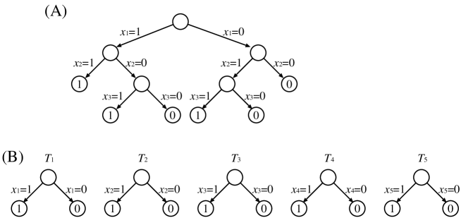
Figure 1: (A) Decision tree representing the majority function on 3 variables, and (B) Random forest (bag of trees) representing the majority function on 5 variables.

3 Bag of trees for the $k$-out-of-$n$ function

In this section, we present a method for constructing a bag of decision trees for representing the $k$-out-of-$n$ function. This method will be used as a kind of subroutine for the main problem.

We begin by defining two types of (sub)trees that will appear in the implementation. We define these trees by describing which inputs they decide to accept, or by the corresponding Boolean formula.

1. The (sub)tree $L_{\ell}(i)$ accepts b if and only if $b_{i}=0$ and it is the leftmost, or second leftmost, or …, the $\ell$-th leftmost 0 in b. I.e., there are at most $1\leq p\leq\ell$ indices $i_{1}\leq\ldots<i_{p}=i$ such that $b_{i_{1}}=\ldots=b_{i_{p}}=0$.

   For example, suppose that $n=3$ (or larger). Then, we have

   $$L_{1}(3) = x_{1}\land x_{2}\land\overline{x_{3}},$$

   $$L_{2}(3) = (x_{1}\land x_{2}\land\overline{x_{3}})\lor(\overline{x_{1}}\land x_{2}\land\overline{x_{3}})\lor(x_{1}\land\overline{x_{2}}\land\overline{x_{3}}).$$

   Note that all of $x_{1},\ldots,x_{b_{i}}$ appear in each conjunction. Then, we can construct a decision tree by simply branching on $x_{1}$ at the root, on $x_{2}$ at the depth 1 nodes, on $x_{3}$ at the depth 2 nodes, and so on. Since it is enough to consider at most

   $$\sum_{i=0}^{\ell-1}\binom{n}{i} \leq O(n^{\ell-1})$$

   combinations and the number of nodes from the root to each leaf is at most $n+1$. $L_{\ell}(i)$ can be represented by a decision tree of size $O(n^{\ell})$, where the size of a decision tree is the number of its nodes.

2. $I_{\ell}(i)$ is a (sub)tree which accepts an input b if and only if $b_{i}=1$ and b contains at least $\ell$ values 1 after $b_{i}$, i.e. $b_{i_{1}}=\ldots=b_{i_{\ell}}=1$ for some $i<i_{1}<\ldots<i_{\ell}\leq 2m-1$ and $b_{j}=0$ for the other $j$s such that $i<j<i_{\ell}$. It will be helpful to visualize the interval $[i_{j},i_{j+1}]$ as a “ones-interval”, with $I_{\ell}(i)$ verifying that, starting at $i$, there are $\ell$ contiguous ones-intervals in the input. We will call these $\ell$ contiguous ones-intervals a “ones-interval of length $\ell$”.

   For example, suppose that $n=5$. Then, we have

   $$I_{1}(2) = (x_{2}\land x_{3})\lor(x_{2}\land\overline{x_{3}}\land x_{4})\lor(x_{2}\land\overline{x_{3}}\land\overline{x_{4}}\land x_{5}),$$

   $$I_{2}(2) = (x_{2}\land x_{3}\land x_{4})\lor(x_{2}\land x_{3}\land\overline{x_{4}}\land x_{5})\lor(x_{2}\land\overline{x_{3}}\land x_{4}\land x_{5}).$$

   Note that each term contains consecutive variables (i.e., $x_{i},x_{i+1},\ldots,x_{j}$ for some $j$) beginning from the same variable $x_{i}$. Then, we can construct a decision tree by simply branching on $x_{i}$ at the root, on $x_{i+1}$ at the depth 1 nodes, on $x_{i+2}$ at the depth 2 nodes, and so on. Since it is enough to consider at most $\binom{n}{\ell}$ terms and the number of nodes from the root to each leaf is at most $n+1$. $I_{\ell}(i)$ can be represented by a decision tree of size $O(n^{\ell+1})$.

As a function of $k$, the trees of $C_{n}(k;\textbf{x})$ are as follows:

1. For $k=m-\ell$ with $1\leq\ell\leq m-1$,

   $T_{1}$	$\cdots$	$T_{\ell}$	$T_{\ell+1}$	$\cdots$	$T_{2m-1}$
   $1$	$\cdots$	$1$	$x_{\ell+1}\lor L_{\ell}(\ell+1)$	$\cdots$	$x_{2m-1}\lor L_{\ell}(2m-1)$

   Note that $T_{i}$ for $i\leq\ell$ corresponds to $x_{i}\lor L_{\ell}(i)$. However, each of them is always 1, and thus 1 is given in this table.

2. For $k=m$,

   $T_{1}$	$\cdots$	$T_{2m-1}$
   $x_{1}$	$\cdots$	$x_{2m-1}$

3. For $k=m+\ell$ with $1\leq\ell\leq m-1$,

   $T_{1}$	$\cdots$	$T_{2m-\ell-1}$	$T_{2m-\ell}$	$\cdots$	$T_{2m-1}$
   $I_{\ell}(1)$	$\cdots$	$I_{\ell}(2m-\ell-1)$	0	$\cdots$	0

For the first case, $T_{i}$ for $i\geq\ell+1$ has To represent this Boolean function by a decision tree, it is enough to add a new root (corresponding to $x_{i}$) to the decision tree for $L_{\ell}(i)$, where the new root has two children: one is a leaf with label 1, the other is the root of the tree for $L_{\ell}(i)$.

Theorem 3.

For fixed $k$, $C_{n}(k;\textbf{x})$ can be represented by a bag of decision trees each of which has size $O(n^{|m-k|+1})$.

Proof.

Let $C^{n}(k;\textbf{x})$ be the bag of decision trees constructed as above. For simplicity, we also represent the result of the majority vote of this bag on input b by $C^{n}(k;\textbf{b})$. We need therefore to prove that $C^{n}(k;\textbf{b})=1$ if and only there are at least $k$ 1’s in b. This is obviously true in case $k=m$.

1. $k=m-\ell$ with $1\leq\ell\leq m-1$.

   Suppose first that b contains at least $k$ 1’s. If b contains at least m 1’s then $C^{n}(k;\textbf{b})$ returns 1 per its definition. Suppose then that b contains $m-p$ 1’s, with $1\leq p\leq\ell$. Noting that b contains more than $\ell$ 0’s, adjoin the indices of the $\ell$ leftmost ones to the set of of indices of the $m-p$ 1’s. The resulting set has size $m-p+\ell\geq m$. Moreover, for each index $i$ in the set $x_{i}\lor L_{\ell}(i)$ has value 1 so that $T_{i}$ returns 1. Hence $C^{n}(k;\textbf{b})=1$.

   To prove the converse assume that $m$ of the trees in $C^{n}(k;\textbf{b})$ return 1 on input b. There are therefore at least $m-\ell$ indices $i_{j}>\ell$ such that $b_{i_{j}}\lor L_{\ell}(i_{j})$ for $i_{j}$. Denote by $p_{0}$ and $q_{0}$ the number of indices $i$ such that $L_{\ell}(i)=1$ for $i\leq\ell$ and $i>\ell$, respectively, and by $p_{1}$ and $q_{1}$ the number of indices $i$ such that $b_{i}=1$ for $i\leq\ell$ and $i>\ell$, respectively. Then $p_{0}+p_{1}=\ell$, $p_{0}+q_{0}\leq\ell$ (by the definition of $L$), and $q_{0}+q_{1}\geq m-\ell$. Hence the number of 1’s in b, $p_{1}+q_{1}$, satisfies

   $$p_{1}+q_{1}=\ell-p_{0}+q_{1}\geq q_{0}+q_{1}\geq m-\ell=k.$$

2. $k=m+\ell$ with $1\leq\ell\leq m-1$.

   If b contains at least $m+\ell$ 1’s at indices $i_{1}<\ldots<i_{m+\ell}$, then each $i_{j}$, $1\leq j\leq m$, is the left endpoint of a ones-interval of length $\ell$ in b. Therefore, for $1\leq j\leq m$, $I_{\ell}(i_{j})=1$ and $T_{i_{j}}$ returns 1. It follows that $C^{n}(k;\textbf{b})=1$.

   To prove the converse assume that $m$ of the trees in $C^{n}(k;\textbf{b})$ return 1 on input b. There are therefore $i_{1}<\cdots<i_{m}$ such that $I_{\ell}(i_{j})=1$, and in particular $b_{i_{j}}=1$. These, together with the $\ell$ additional bits that make $I_{\ell}(i_{m})=1$ show that b contains $k$ 1’s.

Finally, it is seen from the discussions before this theorem that the size of each decision tree is

$$O(n^{\ell})=O(n^{m-k}) \mbox{for $1\leq k<m$}.$$

$$O(1) \mbox{for $k=m$},$$

$$O(n^{\ell+1})=O(n^{k-m+1}) \mbox{for $m<k\leq n$}.$$

Therefore, for each $k$, the size of each decision tree is $O(n^{|m-k|+1})$. ∎

Note that for small $k$, the size given by this theorem is not better than that by a naive construction method, in which all $k$ combinations of variables are represented by $T_{1}$ (as in Figure 1(A)), each of $T_{2},\ldots,T_{m}$ represents 1, each of $T_{m+1},\ldots,T_{2m-1}$ represents 0. Analogously, for large $k$ (close to $n$), the size given by this theorem is not better than that by a naive construction method.

It should also be noted that the case of $k=m-\ell$ and the case of $k=m+\ell$ are not symmetric even if we switch 0 and 1. 0 and 1 are interchanged. Suppose $m=3$ (i.e., $n=2m-1=5$) and $k=m+1=4$. In order to get a positive output, at least four input variables should have value 1. Here, we switch 0 and 1 in the input variables and consider the case of $k=m-1=2$. In order to get a positive output, at least 2 variables should have the switched value 1. This means that at most 3 variables have the switched value 0, corresponding to that at most 3 variables have the original value 1. This example suggests that the cases of $k=m-\ell$ and $k=m+\ell$ are not symmetric.

4 Majority function on $2m-1$ variables by $2m-1-2c$ trees

In this section, we present one of our main results.

Theorem 4.

For any positive integer constant $c$, the majority function on $n=2m-1$ variables can be represented by a bag of $2m-1-2c$ decision trees where the maximum size of each tree is $O(n^{c+1})$.

Proof.

To illustrate the construction we look first at the simplest case, $c=1$. Extending our notation a bit, the majority function on $n=2m-1$ variables can be represented by a bag $B_{2m-3}$ containing $n-2=2m-3$ trees as follows:

$$B_{2m-3}(x_{1},x_{2},\ldots,x_{n})= ((x_{1}x_{2})\land C_{2m-3}(m-2;x_{3},\ldots,x_{n})) \lor$$ (1)

$$((x_{1}\overline{x_{2}})\land C_{2m-3}(m-1;x_{3},\ldots,x_{n})) \lor$$

$$((\overline{x_{1}}x_{2})\land C_{2m-3}(m-1;x_{3},\ldots,x_{n})) \lor$$

$$((\overline{x_{1}}\overline{x_{2}})\land C_{2m-3}(m;x_{3},\ldots,x_{n})).$$

To describe $B_{2m-3}$ explicitly let $T^{-1}_{i}$, $T^{0}_{i}$, and $T^{+1}_{i}$ be the $i$th tree in the bags of $2m-3$ trees representing $C_{2m-3}(m-2;x_{3},\ldots,x_{n})$, $C_{2m-3}(m-1;x_{3},\ldots,x_{n})$, and $C_{2m-3}(m;x_{3},\ldots,x_{n})$, respectively. We also use $T^{-1}_{i}$, $T^{0}_{i}$, and $T^{+1}_{i}$ to denote the Boolean functions corresponding to these trees.

Then the $i$th tree of $B_{2m-3}$, $T_{i}$, is

$$T_{i}=((x_{1}x_{2})\land T^{-1}_{i})\lor((x_{1}\overline{x_{2}})\land T^{0}_{i})\lor((\overline{x_{1}}x_{2})\land T^{0}_{i})\lor((\overline{x_{1}}\overline{x_{2}})\land T^{+1}_{i}).$$

For example, in case $n=5$, we get $3$ decisions trees whose Boolean functions are:

$$((x_{1}x_{2})\land 1)\lor((x_{1}\overline{x_{2}})\land x_{3})\lor((\overline{x_{1}}x_{2})\land x_{3})\lor((\overline{x_{1}}\overline{x_{2}})\land(x_{3}x_{4}\lor x_{3}\overline{x_{4}}x_{5})),$$

$$((x_{1}x_{2})\land(x_{4}\lor x_{3}\overline{x_{4}}))\lor((x_{1}\overline{x_{2}})\land x_{4})\lor((\overline{x_{1}}x_{2})\land x_{4})\lor((\overline{x_{1}}\overline{x_{2}})\land(x_{4}x_{5})),$$

$$((x_{1}x_{2})\land(x_{5}\lor x_{3}x_{4}\overline{x_{5}})\lor((x_{1}\overline{x_{2}})\land x_{5})\lor((\overline{x_{1}}x_{2})\land x_{5})\lor((\overline{x_{1}}\overline{x_{2}})\land 0).$$

The first two levels of the tree $T_{i}$, therefore, branch on the values of $x_{1}$ and $x_{2}$, respectively, with the 4 trees $T^{-1}_{i}$, $T^{0}_{i}$, $T^{0}_{i}$, and $T^{+1}_{i}$ grafted onto the 4 outcomes. According to Section 3 the sizes of $T^{-1}_{i}$, $T^{0}_{i}$, and $T^{+1}_{i}$ are $O(n)$, $O(1)$, and $O(n^{2})$, respectively, so that the theorem holds in this case.

In order to generalize the above discussion to a general constant $c$ we define $P(r,s)$ for $r\geq s$ and given variables $x_{1},\ldots,x_{n}$ by

$$P(r,s) = \bigvee\{z_{1}z_{2}\cdots z_{r}\mid\mbox{($z_{i}=x_{i}$ or $z_{i}=\overline{x_{i}}$ for all $i$)}$$

$$\mbox{and (exactly $s$ of the literals $z_{i}$ are of the form $z_{i}=\overline{x_{i}}$ ) }\},$$

where $P$ is mnemonic for prefix. To illustrate, $P(2,0)=x_{1}x_{2}$, $P(2,1)=x_{1}\overline{x_{2}}\lor\overline{x_{1}}x_{2}$, and $P(2,2)=\overline{x_{1}}\overline{x_{2}}$. Using this notation to generalize the discussion above, we see that the majority function on $n=2m-1$ variables can be represented by

$$\bigvee_{s=0}^{2c}\Bigl{(}P(2c,s)\land C_{2m-1-2c}(m-2c+s;x_{2c+1},x_{2c+2},\ldots,x_{n})\Bigr{)}.$$

Here, we note:

• $C_{2m-1-2c}(m-c-\ell;x_{2c+1},\ldots,x_{n})$ corresponds to the case of $k=m-\ell$ of Section 3,

• $C_{2m-1-2c}(m-c;x_{2c+1},\ldots,x_{n})$ corresponds to the case of $k=m$ of Section 3,

• $C_{2m-1-2c}(m-c+\ell;x_{2c+1},\ldots,x_{n})$ corresponds to the case of $k=m+\ell$ of Section 3.

It is seen from Theorem 3 that each $C_{2m-1-2c}(m-2c+s;x_{2c+1},\ldots,x_{n})$ can be represented by a bag of $2m-1-2c$ trees each of which has $O(n^{c+1})$ nodes. Let $T^{-\ell}_{i}$, $T^{0}_{i}$, and $T^{+\ell}_{i}$ denote the $i$th tree (and also the corresponding Boolean function) in the bag of $2m-1-2c$ trees representing $C_{2m-1-2c}(m-c-\ell;x_{2c+1},\ldots,x_{n})$, $C_{2m-1-2c}(m-c;x_{2c+1},\ldots,x_{n})$, and $C_{2m-1-2c}(m-c+\ell;x_{2c+1},\ldots,x_{n})$, respectively. Then, as in the case of $c=1$, the majority function on $2m-1$ variables can be represented by the majority function on $2m-1-2c$ decision trees in which the $i$th decision tree, $T_{i}$, represents the following Boolean function:

$$T_{i}=\bigvee_{\ell=-c}^{c}\Bigl{(}P(2c,c+\ell)\land T^{\ell}_{i}\Bigr{)}.$$

Constructing $T_{i}$ as in the case $c=1$ yields a tree of size $O(2^{2c}n^{c+1})$ which is $O(n^{c+1})$ for constant $c$. ∎

5 Reducing the number of trees in a general bag of trees while allowing small errors

Unfortunately, the construction given in Section 4 cannot be used to reduce the number of trees in a general random forest (while keeping the tree size polynomial) because conjunction or disjunction of $n$ decision trees each with size $s$ may need a decision tree of size $\Omega(s^{n})$, as discussed in Section 5.1. Therefore, we modify the problem by still asking for a reduction in the number of decision trees in a forest but permitting the transformed forest to make a small number of classification errors, all the while keeping the size of each tree polynomial in $n$.

5.1 Basic idea

Before delving into the details of the construction, we put our finger on the reason why extending Theorem 4 to general random forests is difficult, and then present the central idea for circumventing this difficulty.

It is tempting to deal with the problem of reducing the number of trees in a general bag of trees by modifying the approach that worked for the majority function. After all, the function implemented by the bag is a majority function albeit of trees rather than of variables. Consider, for example, the case $c=1$. Given a bag of trees $B_{2m-1}({\bf x})=\{t_{1}({\bf x}),\ldots,t_{2m-1}({\bf x})\}$ we would like to construct a bag with only $2m-3$ trees, $B_{2m-3}$, using equation (1) while replacing the variables $x_{i}$ on the right hand side by the trees $t_{i}({\bf x})$:

$$B_{2m-3}({\bf x})= (\ (t_{1}({\bf x})t_{2}({\bf x}))\land C_{2m-3}(m-2;t_{3}({\bf x}),\ldots,t_{2m-1}({\bf x}))\ ) \lor$$ (2)

$$(\ (t_{1}({\bf x})\overline{t_{2}({\bf x})}\ )\land C_{2m-3}(m-1;t_{3}({\bf x}),\ldots,t_{2m-1}({\bf x}))\ ) \lor$$

$$(\ (\overline{t_{1}({\bf x})}t_{2}({\bf x}))\land C_{2m-3}(m-1;t_{3}({\bf x}),\ldots,t_{2m-1}({\bf x}))\ ) \lor$$

$$(\ (\overline{t_{1}({\bf x})}\overline{t_{2}({\bf x})})\land C_{2m-3}(m;t_{3}({\bf x}),\ldots,t_{2m-1}({\bf x}))\ ).$$

Following the discussion of Section 3, a tree in the choose bag $C_{2m-3}(m-2;t_{3}({\bf x}),\ldots,t_{2m-1}({\bf x}))$, for example, is of the form $t_{i+2}({\bf x})\lor L_{1}(i+2)$ - where $L_{1}(i+2)$ is a composition of $i$ trees, $L_{1}(i+2)=\wedge_{j=3}^{i+1}(t_{j}({\bf x})\land\overline{t_{i+2}({\bf x})})$ . However, the number of nodes in $L_{1}(i)$ can grow exponentially with the number of trees.

Proposition 5.

Let $T_{1}$ and $T_{2}$ be decision trees with $s_{1}$ and $s_{2}$ nodes, respectively. Then, the conjunction (resp., disjunction) of $T_{1}$ and $T_{2}$ can be represented by a decision tree with $O(s_{1}s_{2})$ nodes.

Proof.

To construct the decision tree for the conjunction of $T_{1}$ and $T_{2}$ replace each leaf of $T_{1}$ that has the label 1 by a copy of $T_{2}$. Clearly the resulting decision tree represents the conjunction of $T_{1}$ and $T_{2}$, and it has $O(s_{1}s_{2})$ nodes. ∎

By repeatedly applying this proposition, the conjunction of $n$ decision trees each having $O(s)$ nodes can be represented by a decision tree of size $O(s^{n})$. As far as we know there is no construction method that requires $o(s^{n})$ size. Therefore, a simple modification of the construction would yield exponential size decision trees even for the case of $c=1$.

To prevent this exponential buildup in the size of the trees we apply the construction of Section 4 to only $K$ carefully chosen trees, while the remaining trees correspond to just single variables. For simplicity of exposition assume for now that the first $K$ trees were chosen, and denote these modified bags by $\hat{B}_{2m-3}$ and $\hat{C}_{2m-3}$, so that equation 2 becomes:

$$\hat{B}_{2m-3}({\bf x})= (\ (t_{1}({\bf x})t_{2}({\bf x}))\land\hat{C}_{2m-3}(m-2;t_{3}({\bf x}),\ldots,t_{2m-1}({\bf x}))\ ) \lor$$ (3)

$$(\ (t_{1}({\bf x})\overline{t_{2}({\bf x})}\ )\land\hat{C}_{2m-3}(m-1;t_{3}({\bf x}),\ldots,t_{2m-1}({\bf x}))\ ) \lor$$

$$(\ (\overline{t_{1}({\bf x})}t_{2}({\bf x}))\land\hat{C}_{2m-3}(m-1;t_{3}({\bf x}),\ldots,t_{2m-1}({\bf x}))\ ) \lor$$

$$(\ (\overline{t_{1}({\bf x})}\overline{t_{2}({\bf x})})\land\hat{C}_{2m-3}(m;t_{3}({\bf x}),\ldots,t_{2m-1}({\bf x}))\ ).$$

Remark 6.

How to choose the $K$ trees is an issue that we will address in the next section. If it turns out that the chosen trees are not the first ones we make them the first ones by reordering.

Example 7.

Consider the reduction of a bag with $n=2m-1=11$ trees to a bag of size $9$, with $K=3$. The trees in $\hat{B}_{9}$ are listed in Table 1. Here $L_{1}(i)=t_{1}\land\cdots\land t_{i-1}\land\overline{t_{i}}$, and $I_{1}(i)=t_{i}\land(t_{i+1}\lor t_{i+2}\lor\cdots\lor t_{K+2})$, for $3\leq i\leq K+1$, with $I_{1}(K+2)=0$. Note that the value of $L_{1}(3)$ is relevant only for ${\bf x}$ such that $t_{1}({\bf x})=t_{2}({\bf x})=1$, and then $t_{3}({\bf x})\lor L_{1}(3)$ is always 1.

Table 1: Representation of the majority function on 11 trees by a bag with 9 trees, $\hat{B}_{9}$, that allows errors, where $K=3$.

prefix	$T_{1}$	$T_{2}$	$T_{3}$	$T_{4}$	$T_{5}$	$T_{6}$	$T_{7}$	$T_{8}$	$T_{9}$
$t_{1}t_{2}$	$t_{3}\lor$	$t_{4}\lor$	$t_{5}\lor$	$t_{6}$	$t_{7}$	$t_{8}$	$t_{9}$	$t_{10}$	$t_{11}$
	$L_{1}(3)$	$L_{1}(4)$	$L_{1}(5)$
$\overline{t_{1}}t_{2}$ (or $t_{1}\overline{t_{2}}$)	$t_{3}$	$t_{4}$	$t_{5}$	$t_{6}$	$t_{7}$	$t_{8}$	$t_{9}$	$t_{10}$	$t_{11}$
$\overline{t_{1}t_{2}}$	$I_{1}(3)$	$I_{1}(4)$	$I_{1}(5)$	$t_{6}$	$t_{7}$	$t_{8}$	$t_{9}$	$t_{10}$	$t_{11}$

For example, an error with $t_{1}({\bf x})=t_{2}({\bf x})=1$ occurs when ${\bf t}({\bf x})=(1,1,1,1,1,1,0,0,0,0,0)$ because only four of the nine transformed trees are 1 (i.e., $\hat{{\bf T}}({\bf x})=(1,1,1,1,0,0,0,0,0)$), and an error with $t_{1}({\bf x})=t_{2}({\bf x})=0$ occurs when ${\bf t}({\bf x})=(0,0,0,0,0,0,1,1,1,1,1)$ because five of the nine transformed trees are 1 (i.e., $\hat{{\bf T}}({\bf x})=(0,0,0,0,1,1,1,1,1)$).

As a prelude to the error analysis detailed in the next section let us examine when $\hat{B}_{9}({\bf x})$ returns an incorrect answer given that $t_{1}({\bf x})=t_{2}({\bf x})=1$. Denote by $S$ the set of ${\bf x}$ such that $t_{1}({\bf x})=t_{2}({\bf x})=1$, and by $S^{1}$, and $S^{0}$, those ${\bf x}\in S$ for which the answer returned by $\hat{B}_{9}({\bf x})$ is the same answer, respectively not the same answer, as the one returned by the original bag $B_{11}({\bf x})$.

According to the definition of $L_{1}(i)$, if on input ${\bf x}$ at least one of the trees $t_{3},t_{4},t_{5}$ returns 0 then the number of 1’s returned by the trees in $\hat{B}_{9}({\bf x})$ is 1 plus the number of 1’s among $t_{3}({\bf x}),\ldots,t_{11}({\bf x})$. Therefore, if at most 2 out of the trees $t_{3}({\bf x}),\ldots,t_{11}({\bf x})$ return 1 (so that $B_{11}({\bf x})=\hat{B}_{9}({\bf x})=0$), or if at least 4 return 1 (so that $B_{11}({\bf x})=\hat{B}_{9}({\bf x})=1$). Moreover, even if 3 of these trees return 1, $\hat{B}_{9}({\bf x})$ still returns the correct answer, $1$, unless $t_{3}({\bf x})=t_{4}({\bf x})=t_{5}({\bf x})=1$.

The probability that $\hat{B}_{9}$ returns an erroneous answer appears, therefore, to be small. However, this issue requires a careful analysis because the configurations of tree values need not be equally likely, even if the inputs x are uniformly distributed. This brings to the forefront the question of how to choose the $K$ trees to which to apply the construction of Section 4. We distill the salient features of the question in the following Problem $P$. Its solution will be detailed in the next section.

Problem $P$: Let ${\cal C}=\{\ 0,1\}^{n}$ be the set of potential tree configurations, and given $p<n$ let ${\cal P}$ be the set of all $\textbf{c}\in{\cal C}$ such that c contains exactly $p$ 1’s. Given $q<p$ and a set of $q$ indices, $J$, let ${\cal P}_{J}\subset{\cal P}$ be the set of all configurations c with the property that $\textbf{c}[j]=1$ for all $j\in J$ (and c contains exactly $p$ 1’s). The problem is to find a $J^{*}$ such that ${\cal P}_{J^{*}}$ has a small probability.

5.2 Details of the construction

We begin with some notations and definitions. Given a bag of decision trees, ${\cal T}=(T_{1},\ldots,T_{n})$, on the set of all binary vectors of length $l$, ${\cal X}=\{{\bf x}_{1},\ldots,{\bf x}_{N}\}$, $N=2^{l}$, let $\textbf{T}({\bf x})=(T_{1}({\bf x}),T_{2}({\bf x}),\ldots,T_{n}({\bf x}))$. The probability distribution on the set of potential tree configurations ${\cal C}=\{\ 0,1\}^{n}$ induced by a probability distribution $D$ on ${\cal X}$ is defined as follows.

Definition 8.

Let $D({\bf x})$ be a probability distribution on ${\cal X}$. The probability that the bag ${\cal T}$ has the configuration ${\bf c}\in{\cal C}$ is

$$\mu({\bf c}) = \sum_{{\bf x}\in{\cal X}:\textbf{T}({\bf x})={\bf c}}D({\bf x}).$$

Note that $\sum_{{\bf c}}\mu({\bf c})=\sum_{{\bf x}}D({\bf x})=1$.

Next we define our error measure. Denote by ${\cal T}({\bf x})$ the majority decision of ${\cal T}$ on ${\bf x}$, i.e. ${\cal T}({\bf x})=\textit{Maj}\circ\textbf{T}({\bf x})$. Our interest is in finding a bag with a smaller number of trees using only the information contained in $\textbf{T}({\bf x})$. In other words, we will consider only functions on ${\cal X}$ of the form ${\cal F}={\cal G}\circ\textbf{T}({\bf x})$.

Definition 9.

Let $D({\bf x})$ be an arbitrary probability distribution on ${\cal X}$. Given a Boolean function ${\cal F}={\cal G}\circ\bf{T}({\bf x})$ on ${\cal X}$ we define its error with respect to ${\cal T}$ by

$$err({\cal F},{\cal T}) = \sum_{\bf{c}\in{\cal C}}\sum_{{\bf x}:{\bf T}({\bf x})=\bf{c}\mbox{ and }{\cal F}({\bf x})\neq{\cal T}({\bf x})}D({\bf x})$$

$$= \sum_{\bf{c}\in{\cal C}:{\cal G}({\bf c})\neq{\textit{Maj}}({\bf c})}\mu({\bf c})$$

Note that $0\leq err({\cal F},{\cal T})\leq 1$.

We use these definitions to address Problem $P$ posed in the previous subsection: for given $q$ is it possible to choose a set of $q$ trees to which to apply the construction of Section 4 so as to guarantee a relatively small probability of error. We denote set of the indices of those trees $J^{*}$.

Lemma 10.

Given $q<p<n$, denote by ${\cal P}=\{{\bf c}_{1},\ldots,{\bf c}_{r}\}$ the set of all $\textbf{c}\in{\cal C}$ such that c contains exactly $p$ 1’s, $r=\binom{n}{p}$. Let ${\cal J}$ denote the set of all sets $J$ consisting of exactly $q$ indices in the range $1,\ldots,n$. For $J\in{\cal J}$ let ${\cal P}_{J}\subseteq{\cal P}$ be the set of all configurations $\bf{c}\in{\cal P}$ with the property that $\textbf{c}[j]=1$ for all $j\in J$. Then there exists a $J^{*}\in{\cal J}$ such that $\mu({\cal P}_{J^{*}})\leq\left({\binom{p}{q}}/{\binom{n}{q}}\right)\mu({\cal P})$.

Proof.

Given $J$ define $\mu_{J}({\bf c}_{i})$ for ${\bf c}_{i}\in{\cal P}$ by

$$\mu_{J}({\bf c}_{i})=\left\{\begin{array}[]{ll}\mu({\bf c}_{i}),&\mbox{if ${\bf c}_{i}[j]=1$ for all $j\in J$},\\ 0,&\mbox{otherwise}.\end{array}\right.$$

Note that for fixed $i$

$$\sum_{J:\ |J|=q}\mu_{J}({\bf c}_{i})=\binom{p}{q}\mu({\bf c}_{i}),$$

so that

$$\sum_{i=1}^{r}\sum_{J:\ |J|=q}\mu_{J}({\bf c}_{i})=\sum_{i=1}^{r}\binom{p}{q}\mu({\bf c}_{i})=\binom{p}{q}\mu({\cal P}).$$

On the other hand,

$$\sum_{i=1}^{r}\sum_{J:|J|=q}\mu_{J}({\bf c}_{i}) = \sum_{J:|J|=q}\sum_{i=1}^{r}\mu_{J}({\bf c}_{i})~{}=~{}\sum_{J:|J|=q}\mu({\cal P}_{J}).$$

It follows that

$$\sum_{J:|J|=q}\mu({\cal P}_{J})=\binom{p}{q}\mu({\cal P}).$$

There are $\binom{n}{q}$ summands $J$s on the left-hand side, hence there is set $J^{*}$ of cardinality $q$ such that

$$\mu({\cal P}_{J^{*}}) \leq\frac{\binom{p}{q}}{\binom{n}{q}}\mu({\cal P}).$$

∎

Theorem 11.

Let ${\cal T}=(t_{1},\ldots,t_{n})$ be a bag of $n=2m-1$ decision trees on ${\cal X}$, and let the size of the largest $t_{i}$ be $s$. Then, for any positive integer constant $K$, there exists a bag of $2m-3$ decision trees on ${\cal X}$, $\hat{B}_{2m-3}$, such that each of its trees has size $O(s^{2K+11})$ and $err({\hat{B}_{2m-3}},{\cal T})\leq{\frac{1}{2^{K}}}$.

Proof.

Let $t_{i}({\bf x})$ be the output of $t_{i}$ on input vector ${\bf x}$. To construct $\hat{B}_{2m-3}$ according to equation (3), we need to first define $\hat{C}_{2m-3}(k;t_{3}({\bf x}),\ldots,t_{2m-1}({\bf x}))$ for $k=m-2,m-1,m$.

1. $\hat{C}_{2m-3}(m-2;t_{3}({\bf x}),\ldots,t_{2m-1}({\bf x}))=\{T^{-}_{1}({\bf x}),\ldots,T^{-}_{2m-3}({\bf x})\}$, where
   $T^{-}_{i}({\bf x})=\left\{\begin{array}[]{ll}t_{2+i}({\bf x})\lor L_{1}(2+i)&\mbox{if }i=1,\ldots,K\\ t_{2+i}({\bf x})&\mbox{if }i=K+1,\ldots,2m-3\end{array}\right.$  
   with $L_{1}(j)=t_{3}({\bf x})\land t_{4}({\bf x})\land\cdots\land t_{j-1}({\bf x})\land\overline{t_{j}({\bf x})}$;

2. $\hat{C}_{2m-3}(m-1;t_{3}({\bf x}),\ldots,t_{2m-1}({\bf x}))=\{t_{3}({\bf x}),\ldots,t_{2m-1}({\bf x})\}$;

3. $\hat{C}_{2m-3}(m;t_{3}({\bf x}),\ldots,t_{2m-1}({\bf x}))=\{T^{+}_{1}({\bf x}),\ldots T^{+}_{2m-3}({\bf x})\}$, where
   $T^{+}_{i}({\bf x})=\left\{\begin{array}[]{ll}I_{1}(2+i)&\mbox{if }i=1,\ldots,K-1\\ 0&\mbox{if }i=K\\ t_{2+i}({\bf x})&\mbox{if }i=K+1,\ldots,2m-3\end{array}\right.$  
   with $I_{1}(j)=t_{j}({\bf x})\land(t_{j+1}({\bf x})\lor\cdots\lor t_{2+K}({\bf x}))$.

Thus $\hat{B}_{2m-3}=\{T_{1}({\bf x}),\ldots,T_{2m-3}({\bf x})\}$ is defined by

$$T_{i}({\bf x}) = (t_{1}({\bf x})\land{t_{2}}({\bf x})\land T_{i}^{-}({\bf x}))\lor(t_{1}({\bf x})\land\overline{t_{2}({\bf x})}\land t_{2+i}({\bf x}))\lor(\overline{t_{1}({\bf x})}\land t_{2}({\bf x})\land t_{2+i}({\bf x}))\lor$$

$$(\overline{t_{1}({\bf x})}\land\overline{t_{2}({\bf x})}\land T_{i}^{+}({\bf x})),$$

and the value of $\hat{B}_{2m-3}$ on an input ${\bf x}$, $\hat{B}_{2m-3}({\bf x})$, is the majority vote of its decision trees, i.e. it is 1 if and only if $m-1$ or more of the $T_{i}({\bf x})$s are satisfied.

We turn next to the analysis of $err({\hat{B}_{2m-3}},{\cal T})$.

Let $h({\bf x})$ and $\hat{h}({\bf x})$ be the number of decision trees in ${\cal T}$, and $\hat{B}_{2m-3}$ respectively, satisfied by ${\bf x}$, i.e. $h({\bf x})=\sum_{i=1}^{2m-1}t_{i}({\bf x})$, and $\hat{h}({\bf x})=\sum_{i=1}^{2m-3}T_{i}({\bf x})$. Also, $h^{-}({\bf x})$ and $h^{+}({\bf x})$ are the number of decision trees $T_{i}^{-}$, and $T_{i}^{+}$, respectively, which return 1 on ${\bf x}$, i.e. $h^{-}({\bf x})=\sum_{i=1}^{2m-3}T_{i}^{-}({\bf x})$, and ${h}^{+}({\bf x})=\sum_{i=1}^{2m-3}T_{i}^{+}({\bf x})$.

We break our analysis up into 3 cases.

Case $t_{1}({\bf x})=t_{2}({\bf x})=1$:

Then $h({\bf x})=2+\sum_{i=3}^{2m-1}t_{i}({\bf x})$, and

$$\hat{h}({\bf x})=h^{-}({\bf x}) = \min\left(1+\sum_{i=3}^{2+K}t_{i}({\bf x}),K\right)+\sum_{i=3+K}^{2m-1}t_{i}({\bf x})$$

$$= \min\left(h({\bf x})-1,h({\bf x})-2+K-\sum_{i=3}^{K+2}t_{i}({\bf x})\right)$$

On the basis of these expressions we distinguish four possibilities:

• if $h({\bf x})\geq m+1$ then $\hat{h}({\bf x})\geq m-1$, so that ${\cal T}({\bf x})=\hat{B}_{2m-3}({\bf x})=1$.

• if $h({\bf x})\leq m-1$ then $\hat{h}({\bf x})\leq m-2$, so that ${\cal T}({\bf x})=\hat{B}_{2m-3}({\bf x})=0$.

• if $h({\bf x})=m$, and in particular ${\cal T}({\bf x})=1$, then

  • if $\sum_{i=3}^{K+2}t_{i}({\bf x})<K$, then $\hat{h}({\bf x})=m-1$ so that also $\hat{B}_{2m-3}({\bf x})=1$.

  • if $\sum_{i=3}^{K+2}t_{i}({\bf x})=K$, then $\hat{h}({\bf x})=m-2$ so that $\hat{B}_{2m-3}({\bf x})=0$.

Only the last case results in an erroneous value of $\hat{B}_{2m-3}({\bf x})$, i.e. an error occurs only when exactly $m-2$ among $(t_{3}({\bf x}),\cdots,t_{2m-1}({\bf x}))$ are 1, and $(t_{3}({\bf x}),\cdots,t_{K+2}({\bf x}))=(1,1,\cdots,1)$, which corresponds to the case of $n=2m-3$, $p=m-2$ and $q=K$ of Lemma 10.

Therefore, the Lemma ensures that there exists a permutation of $t_{3},\ldots,t_{n}$ such that the error in this case is at most

$$\left({\binom{m-2}{K}}/{\binom{2m-3}{K}}\right)\mu({\cal C}_{(1,1)})\leq{\frac{1}{2^{K}}}\mu({\cal C}_{(1,1)}),$$

where we have used the notation.

$${\cal C}_{(\epsilon_{1},\epsilon_{2})}=\{{\bf c}\in{\cal C}\mid{\bf c}[1]=\epsilon_{1},{\bf c}[2]=\epsilon_{2}\},{\rm with}\ \epsilon_{i}\in\{0,1\}$$

Note that $\mu({\cal C}_{(0,0)})+\mu({\cal C}_{(0,1)})+\mu({\cal C}_{(1,0)})+\mu({\cal C}_{(1,1)})=1$.

Case ($t_{1}({\bf x})=1$ and $t_{2}({\bf x})=0$) or ($t_{1}({\bf x})=0$ and $t_{2}({\bf x})=1$):

Then $h({\bf x})=1+\hat{h}({\bf x})=1+\sum_{i=3}^{2m-1}t_{i}({\bf x})$, so that $h({\bf x})\geq m$ if and only if $\hat{h}({\bf x})\geq m-1$.

Case $t_{1}({\bf x})=t_{2}({\bf x})=0$:

Then $h({\bf x})=\sum_{i=3}^{2m-1}t_{i}({\bf x})$, and

$$\hat{h}({\bf x})=h^{+}({\bf x}) = \max\left(-1+\sum_{i=3}^{2+K}t_{i}({\bf x}),0\right)+\sum_{i=3+K}^{2m-1}t_{i}({\bf x})$$

$$= \max\left(h({\bf x})-1,h({\bf x})-\sum_{i=3}^{K+2}t_{i}({\bf x})\right).$$

On the basis of these expressions we distinguish four possibilities:

• if $h({\bf x})\geq m$ then $\hat{h}({\bf x})\geq m-1$, so that ${\cal T}({\bf x})=\hat{B}_{2m-3}({\bf x})=1$.

• if $h({\bf x})\leq m-2$ then $\hat{h}({\bf x})\leq m-2$, so that ${\cal T}({\bf x})=\hat{B}_{2m-3}({\bf x})=0$.

• if $h({\bf x})=m-1$, and in particular ${\cal T}({\bf x})=0$, then

  • if $\sum_{i=3}^{K+2}t_{i}({\bf x})=0$, then $\hat{h}({\bf x})=m-1$ so that $\hat{B}_{2m-3}({\bf x})=1\neq{\cal T}({\bf x})$. $\hat{B}_{2m-3}({\bf x})=1$.

  • if $\sum_{i=3}^{K+2}t_{i}({\bf x})>0$, then $\hat{h}({\bf x})<m-1$ and $\hat{B}_{2m-3}({\bf x})=0$.

In this case, therefore, an error occurs only when exactly $m-2$ among $(t_{3}({\bf x}),\cdots,t_{2m-1}({\bf x}))$ are 0, and $(t_{3}({\bf x}),\cdots,t_{K+2}({\bf x}))=(0,0,\cdots,0)$. This condition corresponds to the case of $n=2m-3$, $p=m-2$ and $q=K$ of Lemma 10 by exchanging the roles of 0 and 1. Hence, the Lemma ensures the existence of a permutation of $t_{3},\ldots,t_{n}$ such that the error in this case is at most

$$\left({\binom{m-2}{K}}/{\binom{2m-3}{K}}\right)\mu({\cal C}_{(0,0)})\leq{\frac{1}{2^{K}}}\mu({\cal C}_{(0,0)}).$$

Since the three cases are mutually independent, the permutations used in the first and the last case need not be the same. We conclude that there exists a bag of $2m-3$ decision trees whose error is at most

$${\frac{1}{2^{K}}}\mu({\cal C}_{(1,1)})+{\frac{1}{2^{K}}}\mu({\cal C}_{(0,0)})\leq{\frac{1}{2^{K}}}.$$

Finally, we analyze the size of the resulting trees. The size can be upper-bounded as $O(s^{Y+1})$ if the number of $\land$ and $\lor$ operators for representing a Boolean function over $t_{1},\ldots,t_{n}$ corresponding to each resulting tree is $Y$. For the case of $t_{1}t_{2}$, the number of operators is at most $2+K$. For the case of $t_{1}\overline{t_{2}}$ (resp., $\overline{t_{1}}t_{2}$), the number of operators is 2. For the case of $\overline{t_{1}}\overline{t_{2}}$, the number of operators is at most $1+K$. Hence, the total number of operators is $(2+K)+2+2+(1+K)+3=2K+10$. It is seen from Proposition 5 that the resulting upper bound of the size of each tree is $O(s^{2K+11})$. ∎

It may be possible to develop a similar construction procedure for the case of $c>1$ by modifying the construction in Theorem 4. However, its probabilistic analysis would be quite difficult. Instead, we use a simple recursive procedure. First, we reduce the number of trees to $2m-3$ using Theorem 11. Then, we reduce the number of trees to $2m-5$ using Theorem 11 again. We repeat this procedure until the number of trees becomes $2m-1-2c$.

Theorem 12.

Let ${\cal T}$ be a bag of $n=2m-1$ decision trees on a set of variables $X=\{x_{1},\ldots,x_{n^{\prime}}\}$, where the size of each decision tree is at most $r$. Then, for any positive integer constants $c$ and $K$, there exists a bag of $2m-1-2c$ decision trees on $X$ such that the size of each bag is $O(r^{(2K+11)^{c}})$ and the error is at most ${\frac{c}{2^{K}}}$.

Proof.

First, we analyze the size of decision trees in a bag. At the first iteration, the size increases from $r$ to $O(r^{2K+11})$ from Theorem 11. Then, this increased size corresponds to the next $r$. Since $K$ is a constant, at the second iteration, the size increases to

$$O((r^{2K+11})^{2K+11}) = O(r^{(2K+11)^{2}}).$$

Since we repeat this procedure $c$ times and $c$ is a constant, the final size is $O(r^{(2K+11)^{c}})$.

Next, we analyze the error. At the first iteration, the error is at most ${\frac{1}{2^{K}}}$ from Theorem 11. Then, we set the weight of the erroneous samples to be 0 and scaling up the weights of the other samples so that the total weight becomes 1. Then, at the second iteration, the error caused by the second iteration is at most ${\frac{1}{2^{K}}}$, where the actual error is not greater than this because the weights are scaled up. Therefore, the total error is at most ${\frac{2}{2^{K}}}$. Since we repeat this procedure $c$ time, the final error is at most ${\frac{c}{2^{K}}}$. ∎

6 Concluding remarks

In this paper, we studied the trade-off between the number of nodes and the number of trees in a bag of decision trees for representing a given bag of $n$ decision trees. As a main result, we showed that the majority function of $n$ variables, that naturally can be represented by a bag of $n$ single node trees, can also be represented by a bag of $n^{\prime}=n-c$ trees, each of polynomial size, in case $c$ is a given constant. If $c$ is not a constant, the derived size is exponential, which is consistent with an exponential lower bound given in [10]. However, the gap between the upper and lower bounds is still large. Therefore, the narrowing of the gap is left as an open problem.

We also considered the general case of representing a given bag of $n$ decision trees using a bag of $n^{\prime}=n-c$ decision trees, for constant $c$. For this case we showed that if the bag is permitted to make classification errors with a small probability, then such a bag with polynomial-size decision trees does indeed exist. The question of whether there exists a bag of $n^{\prime}$ polynomial-size decision trees that makes no errors, is left as an open problem.

References

• [1] Kazuyuki Amano and Masafumi Yoshida. Depth two (n-2)-majority circuits for n-majority. IEICE Trans. Fundam. Electron. Commun. Comput. Sci., 101-A(9):1543–1545, 2018.
• [2] Gilles Audemard, Steve Bellart, Louenas Bounia, FrΓ©dΓ©ric Koriche, Jean-Marie Lagniez, and Pierre Marquis. Trading complexity for sparsity in random forest explanations. In Proceedings of Thirty-Sixth AAAI Conference on Artificial Intelligence (AAAI-2022), pages 5461–5469, 2022.
• [3] GΓ©rard Biau. Analysis of a random forests model. J. Mach. Learn. Res., 13:1063–1095, 2012.
• [4] Leo Breiman. Random forests. Mach. Learn., 45(1):5–32, 2001.
• [5] Anastasiya Chistopolskaya and VladimirΒ V. Podolskii. On the decision tree complexity of threshold functions. Theory Comput. Syst., 66(6):1074–1098, 2022.
• [6] ManuelΒ FernΓ‘ndez Delgado, Eva Cernadas, SenΓ©n Barro, and DinaniΒ Gomes Amorim. Do we need hundreds of classifiers to solve real world classification problems? J. Mach. Learn. Res., 15(1):3133–3181, 2014.
• [7] Christian Engels, Mohit Garg, Kazuhisa Makino, and Anup Rao. On expressing majority as a majority of majorities. SIAM J. Discret. Math., 34(1):730–741, 2020.
• [8] Mikael Goldmann, Johan HΓ₯stad, and AlexanderΒ A. Razborov. Majority gates VS. general weighted threshold gates. Comput. Complex., 2:277–300, 1992.
• [9] AlexanderΒ S. Kulikov and VladimirΒ V. Podolskii. Computing majority by constant depth majority circuits with low fan-in gates. Theory Comput. Syst., 63(5):956–986, 2019.
• [10] SoΒ Kumano and Tatsuya Akutsu. Comparison of the representational power of random forests, binary decision diagrams, and neural networks. Neural Comput., 34(4):1019–1044, 2022.
• [11] StephanΒ Sloth Lorenzen, Christian Igel, and Yevgeny Seldin. On pac-bayesian bounds for random forests. Mach. Learn., 108(8-9):1503–1522, 2019.
• [12] FrΓ©dΓ©ric Magniez, Ashwin Nayak, Miklos Santha, Jonah Sherman, GΓ‘bor Tardos, and David Xiao. Improved bounds for the randomized decision tree complexity of recursive majority. Random Struct. Algorithms, 48(3):612–638, 2016.
• [13] ThaisΒ Mayumi Oshiro, PedroΒ Santoro Perez, and José Augusto Baranauskas. How many trees in a random forest? In Proceedings of 8th International Conference on Machine Learning and Data Mining in Pattern Recognition (MLDM 2012), volume 7376 of Lecture Notes in Computer Science, pages 154–168, 2012.
• [14] Kai-Yeung Siu, Vwani Roychowdhury, and Thomas Kailath. Discrete Mathematics of Neural Networks, Selected Topics. Prentice Hall, 1995.
• [15] Eleonora Testa, Mathias Soeken, LucaΒ Gaetano AmarΓΉ, Winston Haaswijk, and GiovanniΒ De Micheli. Mapping monotone boolean functions into majority. IEEE Trans. Computers, 68(5):791–797, 2019.
• [16] LeslieΒ G. Valiant. A theory of the learnable. Commun. ACM, 27(11):1134–1142, 1984.
• [17] Haoyin Xu, KaleabΒ A. Kinfu, Will LeVine, Sambit Panda, Jayanta Dey, Michael Ainsworth, Yu-Chung Peng, Madi Kusmanov, Florian Engert, ChristopherΒ M. White, JoshuaΒ T. Vogelstein, and CareyΒ E. Priebe. When are deep networks really better than decision forests at small sample sizes, and how?, 2021.
• [18] Zhi-Hua Zhou and JiΒ Feng. Deep forest: Towards an alternative to deep neural networks. In Proceedings of the Twenty-Sixth International Joint Conference on Artificial Intelligence, IJCAI-17, pages 3553–3559, 2017.