Fast Decision Boundary based Out-of-Distribution Detector

Abstract

Efficient and effective Out-of-Distribution (OOD) detection is essential for the safe deployment of AI in latency-critical applications. Recently, studies have revealed that detecting OOD based on feature space information can be highly effective. Despite of their effectiveness, however, exiting feature space OOD methods may incur a non-negligible computational overhead, given their reliance on auxiliary models built from training features. In this paper, we aim to obviate auxiliary models to optimize computational efficiency while leveraging the rich information embedded in the feature space. We investigate from the novel perspective of decision boundaries and propose to detect OOD using the feature distance to decision boundaries. To minimize the cost of measuring the distance, we introduce an efficient closed-form estimation, analytically proven to tightly lower bound the distance. We observe that ID features tend to reside further from the decision boundaries than OOD features. Our observation aligns with the intuition that models tend to be more decisive on ID samples, considering that distance to decision boundaries quantifies model uncertainty. From our understanding, we propose a hyperparameter-free, auxiliary model-free OOD detector. Our OOD detector matches or surpasses the effectiveness of state-of-the-art methods across extensive experiments. Meanwhile, our OOD detector incurs practically negligible overhead in inference latency. Overall, we significantly enhance the efficiency-effectiveness trade-off in OOD detection.

1 Introduction

As machine learning models are increasingly being deployed in the real world, encountering samples out of the training distribution becomes inevitable. Since it is impossible for a classifier to make meaningful predictions on test samples corresponding to classes unseen during training, it becomes crucial to detect Out-of-Distribution (OOD) samples and take necessary precautions accordingly. Since [23] reveals that neural networks tend to be over-confident in OOD samples, a rich line of research work has been focused on mitigating the issue. In particular, some work designs detection scores over model output space for OOD detection [18, 19, 27, 10]. Others turn to utilizing the clustering of In-Distribution (ID) samples in the feature space and further improve the OOD detection performance [29, 17, 28]. For example, [17] fits a multivariate Gaussian over the training features and detects OOD based on the Mahalanobis distance, and [28] detects OOD based on the k-th nearest neighbor (KNN) distance to the training features. While existing feature-space methods demonstrate superior effectiveness, indicating the abundance of OOD information embedded in the feature space, their reliance on auxiliary models built from training features incurs additional computational costs. This poses a challenge for time-critical real-world applications, such as autonomous driving, as the latency of OOD detection is a top priority.

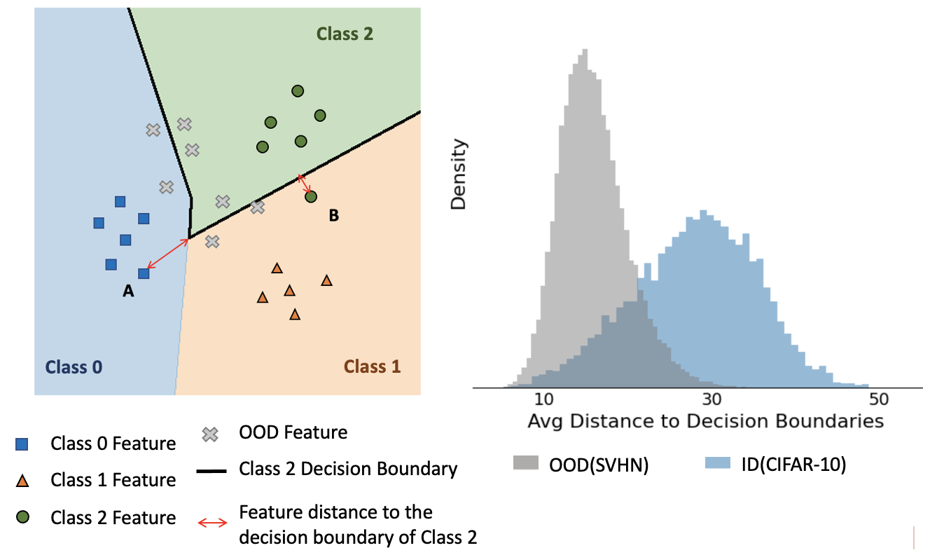
Figure 1: Overview of the Framework. Left: Illustration of the feature distance to decision boundaries on classifier’s penultimate layer. The distance measures the perturbation magnitude required to alter the decision to a class. (See formal definition in Section 3.1). Right: ID features tend to reside further from decision boundaries compared to OOD samples. Distance measurement made using our proposed method (see Section 3.1) on a CIFAR-10 classifier with OOD set SVHN. The average distance is computed per feature across distances to nine non-predicted classes.

In this work, we aim to leverage the rich information embedded in the feature space while optimizing the computational efficiency. To this end, we circumvent building auxiliary models from the training statistics. Instead, we study from the novel perspective of decision boundaries, which naturally summarizes the training statistics. And we begin by asking:

Where do features of ID and OOD samples reside with respect to the decision boundaries?

To answer the question, we first formalize the concept of the feature distance to a class’s decision boundary. We define the distance as the minimum perturbation in feature space to change the classifier’s decision to the selected class, as illustrated in Figure 1 Left. In particular, we focus on the penultimate layer, i.e., the layer before the linear classification head. Due to non-convexity, the distance cannot be readily computed. To minimize the cost of measuring the distance, we introduce an efficient closed-form estimation, analytically proven to tightly lower bound the distance. The feature distance to decision boundaries reflects the difficulty of changing models’ decisions and can quantify model uncertainty in the feature space. As opposed to the output space softmax confidence, our feature-space distance can leverage the abundant information embedded there for OOD detection.

Based on our closed-form distance estimation, we pioneeringly explore OOD detection from the perspective of decision boundaries. Intuitively, features of ID samples would reside further away from the decision boundaries than OOD samples, considering that a classifier is likely to be more decisive in ID samples. We empirically validate our intuition in Figure 1 (Right). Further, we observe ID and OOD can be better separated when compared at equal deviation levels from the mean of training features. Using the deviation level as a regularizer, we design our detection score as a regularized average feature distance to decision boundaries. The lower the score is, the closer the feature resides near decision boundaries, and the more likely that the given sample is OOD.

Thresholding on the detection scores, we have fast Decision Boundary based OOD Detector (fDBD). Our detector is hyperparameter-free and auxiliary model-free, eliminating the cost of tuning parameters and reducing the inference overhead. In addition, our fDBD scales linearly with the number of classes and the feature dimension, theoretically guaranteed to be computationally scalable for large-scale tasks.

With extensive experiments, we demonstrate the superior efficiency and effectiveness of our method across various OOD benchmarks on different classification tasks (ImageNet[3], CIFAR-10[16]), diverse training objectives (cross-entropy $\&$ contrastive loss), and a range of network architectures (ResNet $\&$ DenseNet). Notably, our fDBD consistently achieves or surpasses state-of-the-art OOD detection performance. In the meantime, fDBD maintains inference latency comparable to the vanilla softmax-confidence detector, inducing practically negligible overhead in inference latency. Overall, our method significantly improves upon the efficiency-effectiveness trade-off of existing methods.

We summarize our main contributions below:

• Measuring model uncertainty in the feature space: We formalize the concept of the feature distance to decision boundaries, which quantifies model uncertainty in the feature space. To measure the distance, we introduce an efficient and effective closed-form estimation, providing a beneficial tool for the community.

• Fast decision boundary based OOD detector (fDBD): We establish the first empirical observation that ID features tend to reside further away from decision boundaries than OOD features. From our understanding, we propose a hyperparameter-free, auxiliary model-free, and computationally efficient OOD detector from the novel perspective of decision boundaries.

• Experimental Analysis: We demonstrate across CIFAR-10 and ImageNet benchmarks that our fDBD can achieve or surpass the OOD detection effectiveness of state-of-the-art methods with negligible latency overhead.

• Theoretical Analysis: We establish a theoretical guarantee for the computational efficiency of fDBDthrough complexity analysis. Additionally, we support the effectiveness of our fDBDthrough theoretical analysis.

2 Problem Setting

We consider a data space $\mathcal{X}$, a class set $\mathcal{C}$, and a classifier $f:\mathcal{X}\rightarrow\mathcal{C}$, which is trained on samples i.i.d. drawn from joint distribution $\mathbb{P}_{\mathcal{X}\mathcal{C}}$. We denote the marginal distribution of $\mathbb{P}_{\mathcal{X}\mathcal{C}}$ on $\mathcal{X}$ as $\mathbb{P}^{in}$. And we refer to samples drawn from $\mathbb{P}^{in}$ as In-Distribution (ID) samples. In the real world, the classifier $f$ may encounter $\bm{x}\in\mathcal{X}$ which is not drawn from $\mathbb{P}^{in}$. We refer to such samples as Out-of-Distribution (OOD) samples.

Since a classifier cannot make meaningful predictions on OOD samples from classes unseen during training, it is important to distinguish between In-Distribution (ID) samples and Out-of-Distribution (OOD) samples for the reliable deployment of machine learning models. And for time-critical applications, it is crucial to detect OOD samples promptly to take precautions. Instead of utilizing the clustering of ID features and building auxiliary models as in prior art [17, 28], we alternatively investigate OOD-ness from the perspective of decision boundaries, which inherently captures the training ID statistics.

3 Detecting OOD using Decision Boundaries

To understand the potential of detecting OOD from the perspective of decision boundaries, we ask:

Where do features of ID and OOD samples reside with respect to the decision boundaries?

To this end, we first define the feature distance to decision boundaries in a multi-class setup. We then introduce an efficient and effective method for measuring the distance through closed-form estimation. Using our distance method, we observe the ID features tend to reside further away from the decision boundaries. And we propose a decision boundary-based OOD detector accordingly. Our detector is post-hoc and can be built on top of any pre-trained classifiers, agnostic to model architecture, training procedure, and OOD types. In addition, our detector is hyperparameter-free, auxiliary model-free, and computationally efficient.

3.1 Feature Distance to Decision Boundaries

We now formalize feature distance to the decision boundaries. We denote the last layer function of $f$ as $f_{-1}:\mathcal{Z}\rightarrow\mathcal{C}$, which maps a penultimate feature vector $\bm{z}$ into a class $c$. Since $f_{-1}$ is linear, we can express $f_{-1}$ as:

$$f_{-1}(\bm{z})=\arg\max_{c\in\mathcal{C}}\bm{w}_{c}^{T}\bm{z}+b_{c},$$

where $\bm{w}_{c}$ and $b_{c}$ are parameters of the linear classifier corresponding to class $c$.

Definition 1.

On the penultimate space of classifier $f$, we define the $L2$-distance of feature embedding $\bm{z_{x}}$ for sample $\bm{x}$ to the decision boundary of class $c$, where $c\neq f(\bm{x})$, as:

$$D_{f}(\bm{z_{x}},c)=\inf_{\{\bm{z^{\prime}}:f_{-1}(\bm{z^{\prime}})=c\}}\left\lVert\bm{z_{x}}-\bm{z^{\prime}}\right\rVert_{2}.$$

Here, $\{\bm{z^{\prime}}:f_{-1}(\bm{z^{\prime}})=c\}$ is the decision region of class $c$ in the penultimate space. Therefore, the distance we defined is the minimum perturbation required to change the model’s decision to class $c$, providing a measure that quantifies the difficulty of altering the model’s decision.

As the decision region is non-convex in general as shown in Figure 1, the feature distance to the decision boundaries in Definition 1 does not have a closed-form solution and cannot be readily computed. To circumvent computationally expensive iterative estimation, we relax the decision region and propose an efficient and effective estimation method for measuring the distance.

Theorem 1.

On the penultimate space of classifier $f$, the $L2$-distance of feature embedding $\bm{z_{x}}$ for sample $\bm{x}$ to the decision boundary of class $c$, where $c\neq f(\bm{x})$, i.e. $D_{f}(\bm{z_{x}},c)$, is tightly lower bounded by

$$\tilde{D}_{f}(\bm{z_{x}},c)\coloneqq\frac{|(\bm{w}_{f(\bm{x})}-\bm{w}_{c})^{T}\bm{z_{x}}+(b_{f(\bm{x})}-b_{c})|}{\left\lVert\bm{w}_{f(\bm{x})}-\bm{w}_{c}\right\rVert_{2}},$$ (1)

where $\bm{z_{x}}$ is the penultimate space feature embedding of $\bm{x}$ under classifier $f$, $\bm{w}_{f(\bm{x})}$ and $b_{f(\bm{x})}$ are parameters of the linear classifier corresponding to the predicted class $f(\bm{x})$.

Proof.

Let

$$\mathcal{Z}_{c} :=\{\bm{z^{\prime}}:f_{-1}(\bm{z^{\prime}})=c\}$$

$$=\{\bm{z^{\prime}}:\bm{w}_{c}^{T}\bm{z^{\prime}}+b_{c}>\bm{w}_{c^{\prime}}^{T}\bm{z^{\prime}}+b_{c^{\prime}}\ \forall c^{\prime}\neq c\};$$

$$\mathcal{Z}_{c}^{\prime} :=\{\bm{z^{\prime}}:\bm{w}_{c}^{T}\bm{z^{\prime}}+b_{c}>\bm{w}_{f(\bm{x})}^{T}\bm{z^{\prime}}+b_{f(\bm{x})}\}.$$

Observe that $\mathcal{Z}_{c}\subseteq\mathcal{Z}_{c}^{\prime}$. Therefore, we have

$$D_{f}(\bm{z_{x}},c)=\inf_{\bm{z^{\prime}}\in\mathcal{Z}_{c}}\left\lVert\bm{z^{\prime}}-\bm{z_{x}}\right\rVert_{2}\geq\inf_{\bm{z^{\prime}}\in\mathcal{Z}_{c}^{\prime}}\left\lVert\bm{z^{\prime}}-\bm{z_{x}}\right\rVert_{2}.$$ (2)

Note that geometrically $\inf_{\bm{z^{\prime}}\in\mathcal{Z}_{c}^{\prime}}\left\lVert\bm{z^{\prime}}-\bm{z_{x}}\right\rVert_{2}$ represents the $l_{2}$ distance from $\bm{z_{x}}$ to hyperplane

$$(\bm{w}_{f(\bm{x})}-\bm{w}_{c})^{T}\bm{z}+(b_{f(\bm{x})}-b_{c})=0,$$ (3)

and thus

$$\inf_{\bm{z^{\prime}}\in\mathcal{Z}_{c}^{\prime}}\left\lVert\bm{z^{\prime}}-\bm{z_{x}}\right\rVert_{2}=\frac{|(\bm{w}_{f(\bm{x})}-\bm{w}_{c})^{T}\bm{z_{x}}+(b_{f(\bm{x})}-b_{c})|}{\left\lVert\bm{w}_{f(\bm{x})}-\bm{w}_{c}\right\rVert_{2}}.$$ (4)

Combining Eqn. (4) with Eqn. (2), we conclude that Eqn. (1) lower bounds $D_{f}(\bm{z_{x}},c)$.

We now show that equality in Eqn. (2) holds for class $c_{2}$, corresponding to the nearest hyperplane to the sample embedding $\bm{z_{x}}$, i.e.,

$$c_{2}:=\arg\min_{c\in\mathcal{C},c\neq f(\bm{x})}\inf_{\bm{z^{\prime}}\in\mathcal{Z}_{c}^{\prime}}\left\lVert\bm{z^{\prime}}-\bm{z_{x}}\right\rVert_{2}.\vspace{-1.5mm}$$ (5)

Let the projection of $\bm{z}_{\bm{x}}$ on the nearest hyperplane be $\bm{p}_{\bm{x}}$. From Eqn. (5), for all $c\notin\{c_{2},f(\bm{x})\}$, we have

$$\left\lVert\bm{p}_{\bm{x}}-\bm{z_{x}}\right\rVert_{2}=\inf_{\bm{z^{\prime}}\in\mathcal{Z}_{c_{2}}^{\prime}}\left\lVert\bm{z^{\prime}}-\bm{z_{x}}\right\rVert_{2}\leq\inf_{\bm{z^{\prime}}\in\mathcal{Z}_{c}^{\prime}}\left\lVert\bm{z^{\prime}}-\bm{z_{x}}\right\rVert_{2}.$$ (6)

Consequently, we have $\bm{p_{x}}\in{\mathcal{Z}^{\prime}_{c}}^{\complement}$, i.e. $\bm{w}_{c}^{T}\bm{p_{x}}+b_{c}\leq\bm{w}_{f(\bm{x})}^{T}\bm{p_{x}}+b_{f(\bm{x})}$ for any $c\notin\{f(\bm{x}),c_{2}\}$. Intuitively, as all other hyperplanes are further away from $\bm{z_{x}}$ than $\bm{p_{x}}$, $\bm{p_{x}}$ and $\bm{z_{x}}$ must fall on the same side of each hyperplane. Therefore, $p_{\bm{x}}$ falls within the closure of $\mathcal{Z}_{c_{2}}$, i.e. $p_{\bm{x}}\in\overline{\mathcal{Z}}_{c_{2}}$. It follows that

$$\left\lVert\bm{p_{x}}-\bm{z_{x}}\right\rVert_{2}\geq\inf_{\bm{z^{\prime}}\in\mathcal{Z}_{c_{2}}}\left\lVert\bm{z^{\prime}}-\bm{z_{x}}\right\rVert_{2}.$$ (7)

Combining Eqn. (6) Eqn. (7), we see that equality holds in Eqn. (2) for $c=c_{2}$. Therefore, we conclude that Eqn. (1) tightly lower bounds $D_{f}(\bm{z_{x}},c)$ ∎

Effectiveness of Distance Measure Besides the theoretical guarantee of the effectiveness given in Theorem 1, we also verify empirically that our estimation method achieves high precision with a relative error of less than $1.5\%$. More details are available in Appendix 12.

Efficiency of Distance Measure Analytically, Eqn. (1) can be computed in constant time on top of the inference process. Specifically, the numerator in Eqn. (1) calculates the absolute difference between corresponding logits, generated during model inference. And the denominator takes a finite number of $|\mathcal{C}|\times(|\mathcal{C}|-1$) possible values, which can be pre-computed and retrieved in constant time during inference. Empirically, our method incurs negligible inference overhead. In particular, on a Tesla T4 GPU, the average inference time on the CIFAR-10 classifier is 0.53ms per image with or without computing the distance using our method. In contrast, the alternative way of estimating the distance through iterative optimization takes 992.2ms under the same setup. This empirically validates the efficiency of our proposed estimation. For experiment details, see Appendix 12.

For the rest of the paper, we use our closed-form estimation of the feature distance to decision boundaries, formulated in Eqn. (1), for our OOD detection methods.

Table 1: fDBD achieves superior performance with negligible latency overhead on CIFAR-10 OOD benchmark. Evaluated with FPR95, AUROC, and inference latency. $\uparrow$ indicates that larger values are better and vice versa. Best performance highlighted in bold.

3.2 Fast Decision Boundary based OOD Detector

We now study OOD detection from the perspective of decision boundaries. Recall that the feature distance to decision boundaries measures the minimum perturbation required to change the classification. Therefore, the feature distance reflects the difficulty of changing the model’s decision. Given that a model tends to be more certain on ID samples, we hypothesize that ID features are more likely to reside further away from the decision boundaries compared to OOD features. In Figure 3 (Left), we validate this hypothesis by averaging the feature distance to decision boundaries. A further validation on the feature distance to each individual decision boundary is in Appendix 11.

Going one step further, we want to investigate the overlapping region of ID/OOD measured by average distance to decision boundaries. To this end, we plot Figure 2 where we group ID and OOD samples into buckets based on their deviation from the mean of training features. For each group, we plot the mean and variance of the average distance to decision boundaries. Looking into Figure 2, we discover that the average feature distance to decision boundaries of both ID and OOD samples increases as features deviate from the mean of training features. This leads to OOD samples in a higher deviation level cannot be well distinguished by ID samples that fall into a lower deviation level. In contrast, within the same deviation level, OOD can be much better separated from ID samples. We provide theoretical insights of our observation in Section 5.

Based on this understanding, we design our OOD detection score as the average feature distances to decision boundaries, regularized by the feature distance to the mean of training features:

$$\mathtt{regDistDB}\coloneqq\frac{1}{|\mathcal{C}|-1}\sum_{\begin{subarray}{c}c\in\mathcal{C}\end{subarray},\ c\neq f(\bm{x})}\frac{\tilde{D}_{f}(\bm{z_{x}},c)}{\|\bm{z_{x}}-\bm{\mu}_{train}\|_{2}},$$ (8)

where $\tilde{D}_{f}(\bm{z_{x}},c)$ is the estimated feature distance defined in Eqn. (1) and $\bm{\mu}_{train}$ denotes the mean of training features. As shown in Figure 3, the regularized distance score enhances the ID/OOD separation as the score approximately compares ID and OOD samples at the same deviation levels. By applying a threshold on $\mathtt{regDistDB}$, we introduce the fast Decision Boundary based OOD Detector (fDBD), which identifies samples below the threshold as OOD.

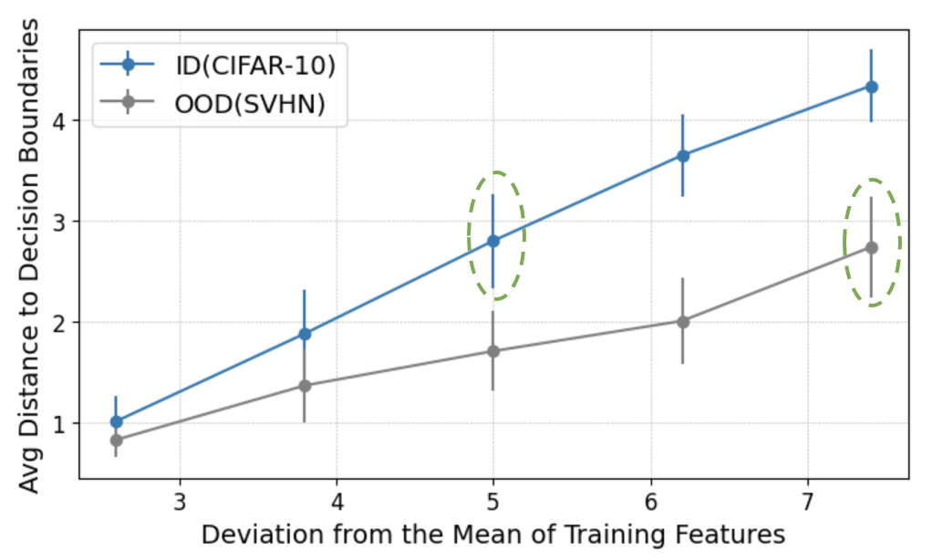
Figure 2: Intuition for comparing ID and OOD at Equal Deviation Levels. The average feature distance from decision boundaries increases as features deviate from the mean of training features. Features are grouped by deviation levels with group mean and variance displayed. The circled ID/OOD groups cannot be distinguished based on their average distance to decision boundaries while being effectively separable at their own deviation levels.

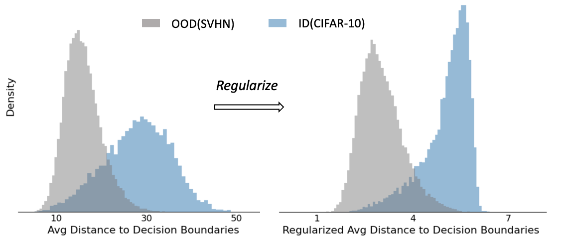
Figure 3: Regularization enhances ID/OOD seperation. Left: Histograms of ID/OOD features based on the average distance to decision boundaries. Right: Histograms of ID/OOD features based on the regularized average distance to decision boundaries, comparing ID and OOD features at equal deviation levels from the mean of training features.

It’s worth noticing that our fDBD is hyper-parameter-free and auxiliary-model-free. In contrast to many existing approaches [18, 17, 28], our method eliminates the pre-inference cost of tuning hyper-parameter and the potential requirement for additional data. Benefiting from our closed-form distance measuring method, fDBD is computationally efficient as well. In particular, the computational time of fDBD scales linearly with the number of training classes $|\mathcal{C}|$ and the dimension of penultimate layer $P$, indicating a negligible increase in cost when scaling up to larger datasets and models. Recall that computing $\tilde{D}_{f}(\bm{z_{x}},c)$ takes constant time, while computing $\|\bm{z_{x}}-\bm{\mu_{G}}\|_{2}$, the denominator of $\mathtt{regDistDB}$, has time complexity $O(P)$. Overall, fDBD has time complexity $O(|\mathcal{C}|+P)$. We will further demonstrate the efficiency of fDBD through experiments in Section 4.

4 Experiments

In this section, we demonstrate the superior efficiency and effectiveness of fDBD across OOD Benchmarks To empirically study the efficiency of OOD detectors, we report the per-image inference latency (in milliseconds) evaluated on a Tesla T4 GPU. To evaluate the effectiveness, we use two widely used recognized metrics in the literature: the False Positive rate at $95\%$ true positive rate (FPR95) and the Area Under the Receiver Operating Characteristic Curve (AUROC). A lower FPR95 score indicates better performance, whereas a higher AUROC value indicates better performance. We refer readers to Appendix 9 for detailed experimental setups.

4.1 Evaluation on CIFAR-10 Benchmarks

In Table 1, we present the evaluation of baselines and our fDBD on CIFAR-10 OOD benchmark. The CIFAR-10 classifier we evaluated on has a ResNet-18 backbone, was trained under cross-entropy loss, and achieves an accuracy of 94.21%.

Datasets On the CIFAR-10 OOD benchmark, we use the standard CIFAR-10 test set with 10,000 images as ID test samples. For OOD samples, we consider common OOD benchmarks: CIFAR-100, SVHN, LSUN-crop, LSUN-resize [37], iSUN [35], Places365 [38], and Texture [2]. All images are of size $32\times 32$.

Baselines We compare our method with 5 baseline methods which utilize the input or feature space information for OOD detection. In particular, MSP [9], ODIN [18], and Energy [19] design OOD score functions on the model output. MDS [17] and KNN [28], on the other hand, utilize the clustering of ID samples in the feature space and build an auxiliary model for OOD detection. Our method fDBD also utilizes information in the feature space. Yet from a decision boundary perspective, we eliminate the need for an auxiliary model. Moreover, our fDBD, as well as MSP and Energy, is hyper-parameter free; whereas the rest of the baselines requires tuning hyper-parameter prior to inference.

Table 2: fDBD achieves superior performance with negligible latency overhead on ImageNet OOD benchmark. Evaluated with FPR95, AUROC, and inference latency. $\uparrow$ indicates that larger values are better and vice versa. Best performance highlighted in bold.

OOD Detection Performance In Table 1, we compare fDBD with the baselines. Overall, fDBD on average improves state-of-art performance both in terms of FPR95 and AUROC scores. In addition, fDBD induces minimal computational overhead. As a reference, under the same setup, the original classifier’s inference without any OOD detection mechanism reports 0.53ms per image. In the meantime, inference with fDBDalso reports 0.53ms per image, indicating practically negligible overhead induced by our algorithm. The computational efficiency of fDBDis a result of our proposed distance measuring method, which induces practically negligible overhead on top of inference as demonstrated in Section 3.1. Between our fDBDand the baselines, we highlight two groups of comparisons:

• fDBD v.s. MSP Both fDBD and MSP aim to detect OOD based on model uncertainty. Specifically, MSP characterizes model uncertainty using model softmax confidence in the output space, whereas our fDBD quantifies model uncertainty in the feature space using feature distance to decision boundaries. Looking into the performance of two methods in Table 1, our fDBD reduces the average FPR95 by 29.70%, which is a relatively 52.36% reduction in error. The significant improvement aligns with our intuition that substantial information is embedded in the feature space for OOD detection and that capturing uncertainty in the feature space rather than the output space improves the OOD detection performance.

• fDBD v.s. KNN We compare to KNN under the same setup as in the original paper [28] with the number of nearest neighbor $k$ set to the suggested value $50$ and all 50,000 training data are used for the nearest neighbor search. On the same model, our method achieves an FPR95 score of $27.02\%$, improving over that of KNN $29.31$. More importantly, KNN reports an average inference time of $1.93ms$ per image, inducing a noticeable overhead in comparison to the original inference time of $0.53ms$ per image. This is in line with our intuition that inference from the k nearest neighbor auxiliary model induces computational overhead. On the contrary, our auxiliary model-free fDBDoperates with minimal overhead and significantly reduces the latency.

4.2 Evaluation on ImageNet Benchmarks

In Table 2 , we further compare the efficiency and effectiveness of our fDBD and baselines on larger scale ImageNet OOD Benchmarks. The ImageNet classifier we evaluated with has a ResNet-50 backbone, was trained under cross-entropy loss, and achieves an accuracy of 76.65%.

Datasets $\&$ Baselines We use 50,000 ImageNet validation images in the standard split as ID test samples. Following [13, 28], we use Places365 [38], iNaturalist [31], and SUN [34] with non-overlapping classes w. r. t. ImageNet as OOD samples. All images are of size $224\times 224$.

In the meantime, we compare to the same baselines introduced in Section 4.1 for CIFAR-10. For KNN, we consider two sets of hyper-parameters reported in the original paper [28]: $\alpha=100\%$ refers to searching through all training data for $k=1000$ nearest neighbors; $\alpha=1\%$ refers to searching through sampled $1\%$ of training data for $10$ nearest neighbors.

OOD Detection Performance As we observe from Table 2, fDBD outperforms all baselines in both average FPR95 and average AUROC on ImageNet OOD Benchmarks. This demonstrates fDBD consistently maintains its superior effectiveness in OOD detection on large-scale datasets. In addition, fDBD remains computationally efficient in ImageNet OOD detection. This aligns with our observation on CIFAR-10 benchmarks and supports our analysis that fDBD scales linearly with class and dimension, keeping the computational manageable for OOD detection on large models and datasets.

4.3 Evaluation under Contrastive Learning

To examine the generalizability of our proposed method beyond classifiers trained with cross-entropy loss, we further experiment with a contrastive learning scheme. We consider four baseline methods particularly competitive under contrastive loss: $\mathtt{CSI}$ [29], $\mathtt{SSD+}$ [25], and $\mathtt{KNN+}$  [28]. In Table 3, we evaluate fDBD, $\mathtt{CSI}$, $\mathtt{SSD+}$, and $\mathtt{KNN+}$ on a CIFAR-10 classifier with ResNet18 backbone trained with supervised contrastive (supcon) loss [15]. The classifier achieves an accuracy of $94.64\%$.

Table 3: fDBD achieves superior performance with negligible latency overhead under Contrastive Learning Scheme. Evaluated with FPR95, AUROC, and inference latency. $\uparrow$ indicates that larger values are better and vice versa. Best performance highlighted in bold.

Table 4: fDBD achieves superior performance with negligible latency overhead on DenseNet. Evaluated with FPR95, AUROC, and inference latency. $\uparrow$ indicates that larger values are better and vice versa. Best performance highlighted in bold.

From Table 3, we observe that under a contrastive training scheme, our proposed detector still exhibits state-of-the-art effectiveness. In addition, our fDBD induces less computational overhead than other competitive baselines. Looking into Table 3 with Table 1, we observe that OOD detection performance significantly improves when the classifier is trained with contrastive loss. This is in line with the observation in [28] that ID and OOD features are better separated under a contrastive learning scheme than the classical cross-entropy loss.

4.4 Evaluation on DenseNet

So far our evaluation shows that fDBD exhibits superior efficiency and effectiveness on the ResNet backbone across OOD Benchmarks over different classification tasks and classifiers under different training objectives. We now extend our evaluation to DenseNet [12]. The CIFAR-10 classifier we evaluated achieves a classification accuracy of $94.53\%$. We consider the same OOD test sets as in Section 4.1 for CIFAR-10. The performance shown in Table 4 further indicates the effectiveness and efficiency of our proposed detector across different network architectures.

4.5 Ablation Study

4.5.1 Effect of Regularization

Previously, we illustrate in Figure 3 Left and Right that regularization enhances the ID/OOD separation as the regularized score approximately compares ID and OOD samples at the same deviation levels We now quantitatively study the effect in Table 5. Specifically, we compare the performance of OOD detection on ImageNet benchmarks using the regularized average distance $\mathtt{regDistDB}$, the regularization term $\|z-\mu_{train}\|_{2}$, as well as the un-regularized average distances, namely $\mathtt{avgDistDB}\coloneqq\|z-\mu_{train}\|_{2}\ \mathtt{regDistDB}$ as detection scores respectively. We report the performance in AUROC scores Table 5 and FPR95 in Appendix 13. Aligning with Figure 2, $\|z-\mu_{train}\|_{2}$ alone does not necessarily distinguish between ID and OOD samples, as indicated by AUROC scores around 50. However, regularization with respect to $\|z-\mu_{train}\|_{2}$ approximates fair comparison at equal deviation from $\mu_{train}$. And as shown in Table 5, $\mathtt{regDistDB}$ improves the performance of $\mathtt{avgDistDB}$ and achieves higher AUROC scores. This further supports our intuitions for regularization in Section 3.

4.5.2 Effect of Individual Distances

In our fDBD , we detect OOD by considering feature distances to the decision boundaries, averaging over all classes except the predicted class. Notably, fDBD operates as a hyperparameter-free method, and we do not tune the number of distances in our experiments. Nevertheless, we perform an ablation study to understand the effect of individual distances on the OOD detection performance.

Table 5: Regularization enhances the effectiveness of OOD detection. AUROC scores reported on ImageNet Benchmarks (higher is better). $\mathtt{regDistDB}$ outperforms $\mathtt{avgDistDB}$.

To align across samples predicted as different classes, we sort per sample the feature distances to decision boundaries. We then detect OOD considering the average of the t the top-$k$ smallest distances. Specifically, $k=1$ corresponds to the detecting score being the ratio between the feature distance to the closest decision boundary and the feature distance to the mean of training features. And $k=9$ on CIFAR-10 and $k=999$ on ImageNet correspond to our original detection scores $\mathtt{regDistDB}$ (see Eqn. (8)), where we average over all distances for OOD detection.

In Figure 4, we plot the corresponding FPR95 and AUROC score against the number of distances $k$ used for OOD detection. Looking into Figure 4, the performance improves with increasing number of $k$. This justifies our design of fDBD as a hyper-parameter-free method that deploys all distances for OOD detection.

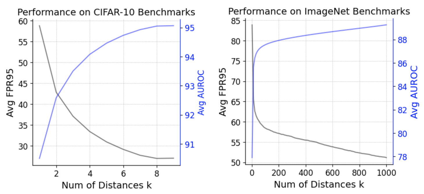
Figure 4: Ablation on Individual Distances. Left: CIFAR-10 Benchmark performance improves with an increasing number of distances. Right: ImageNet Benchmark performance improves with an increasing number of distances. The performance supports the use of all distances in our hyper parameter-free fDBD.

5 Theoretical Analysis

In this section, we provide theoretical analysises to shed light on our observation and algorithm design in Section 3.

Setups

We consider a binary classifier with a 2-D penultimate layer. Following [17], we model the ID feature distribution as a Gaussian mixture of two components: $N(\bm{\mu}_{0},\sigma_{0})$ and $N(\bm{\mu}_{1},\sigma_{1})$. We consider the case where the standard deviation is equivalent $\sigma_{0}=\sigma_{1}=\sigma$ and the two classes are well separated at their three standard deviations percentiles, i.e. $\|\bm{\mu}_{0}-\bm{\mu}_{1}\|>6\sigma$. The mean of the ID distribution is therefore $\bm{\mu}\doteq\bm{\mu}_{0}+\bm{\mu}_{1}$. And the decision boundary between two classes is then $\mathcal{S}\doteq\{\bm{z}:\bm{z}\cdot(\bm{\mu_{0}}-\bm{\mu_{1}})=\frac{\|\bm{\mu}_{0}\|^{2}-\|\bm{\mu}_{1}\|^{2}}{2}\}$.

Following [28], we assume that OOD features reside outside the dense region of ID feature distribution. In particular, we consider the dense region of the ID distribution as the region within two standard deviations from each class mean $\mathcal{I}\doteq\{\bm{z}:\|\bm{z}-\bm{\mu}_{0}\|\leq 2\sigma\}\cup\|\bm{z}-\bm{\mu}_{1}\|\leq 2\sigma\}$.

Main Result

In Section 3, we empirically observed that the feature distance to decision boundaries increases as features deviate from the mean of training features $\bm{\mu}_{train}$. We are inspired to compare ID/OOD at equal deviation levels and design our detection score accordingly. Essentially, $\bm{\mu}_{train}$ is an empirical estimation of $\bm{\mu}$, the mean of ID feature distribution.

To shed light on our observation, we now show that the feature distance to the decision boundary $d(\mathcal{S},z)$ increases on average as $z$ deviates from $\bm{\mu}$.

Proposition 1.

Consider features of equal distance $r$ to the ID distribution mean $\mathcal{E}_{r}\doteq\{\bm{z}:\|\bm{z}-\bm{\mu}\|=r\}$. For any $r_{0}<r_{1}$, we have:

$$\frac{1}{2\pi r_{0}}\int_{z\in\mathcal{E}_{r_{0}}}d(S,z)\,\mathrm{d(z)}<\frac{1}{2\pi r_{1}}\int_{z\in\mathcal{E}_{r_{1}}}d(S,z)\,\mathrm{d(z)}$$ (9)

We then show that at an equal distance from $\mu$, ID features tend to have a larger distance than OOD features.

Proposition 2.

Consider features of equal distance $r$ to the ID distribution mean, where $\sigma<r<5\sigma$ We have

$$\frac{1}{2\pi r\arctan(2\sigma/r)}\int_{z\in\mathcal{I}\cap\mathcal{E}_{r}}d(S,z)\,\mathrm{d(z)}$$ (10)

$$>\frac{1}{2\pi r\arctan(r/2\sigma)}\int_{z\in\mathcal{I}^{\complement}\cap\mathcal{E}}d(S,z)\,\mathrm{d(z)}$$

See proofs in Appendix 8.

6 Related Work

An extensive body of research work has been focused on developing OOD detection algorithms and a comprehensive survey of recent work can be found in [36]. Particularly, one line of work is post-hoc and builds upon pre-trained models. For example, [18, 10, 19, 27, 26] design OOD score over the output space of a classifier. Meanwhile, a line of work [17, 28, 22] measures OOD-ness with a focus on the feature space. Some recent work further combines input and output space information for OOD detection. For example, [32] constructs a virtual logit combining the feature and logits, whereas [5] shapes the feature space activation before computing the output space score. Moreover, [14] explores OOD detection from the gradient space. Our work builds on the feature space and investigates from the largely under-explored perspective of decision boundaries.

Another line of work explores the regularization of OOD detection in training. For example, [4, 11] propose OOD-specific architecture whereas [33, 13, 21] design OOD-specific training loss. In particular, [29] brings attention to representation learning for OOD detection and proposes an OOD-specific contrastive learning scheme. In addition, [30, 7] explores methods for constructing virtual OOD samples to facilitate OOD-aware training. Recently, [8] reveals that finetuning a visual transformer [6] with OOD exposure significantly can improve OOD detection performance. Our work does not assume specific training schemes or architecture and we do not belong to this school of work.

7 Conclusion

In this work, we propose an effective and efficient OOD detector. To utilize feature space information efficiently, we study from the perspective of decision boundaries and we propose an efficient and effective method for measuring the distance. Utilizing the relationship between OOD-ness and features distance to decision boundaries, we design a decision boundary-based OOD detector, achieving state-of-the-art effectiveness while inducing negligible latency overhead. We hope our proposed tool and algorithm can inspire future work to explore model uncertainty from the perspective of decision boundaries for OOD detection and other research problems such as adversarial robustness and domain generalization.

Supplementary Material

8 Proof for Section 5

Proof of Proposition 1

Consider polar coordinates centered at the mean of ID feature distribution $\bm{\mu}$. For $\forall\bm{z}\in\mathcal{E}_{r}$, we then have $\bm{z}=(\bm{\mu}+r\sin t,\bm{\mu}+r\cos t)$. Therefore, we have

$$\frac{1}{2\pi r}\int_{z\in\mathcal{E}_{r}}d(S,z)\,\mathrm{d(z)}=\frac{1}{\pi}\int^{\pi}_{0}r\sin t\mathrm{d}t=\frac{2}{\pi}r$$ (11)

As Equation 11 increases with $t$, we conclude that Proposition 1 holds.

Proof of Proposition 2

Following the same polar coordinate system, we have

$$\text{LHS}= \frac{1}{2\pi r\arctan(2\sigma/r)}\int_{z\in\mathcal{I}\cap\mathcal{E}_{r}}d(S,z)\,\mathrm{d(z)}$$ (12)

$$= \frac{1}{2\arctan(2\sigma/r)}\int^{\frac{\pi}{2}+\arctan(2\sigma/r)}_{\frac{\pi}{2}-\arctan(2\sigma/r)}r\ \sin t\ \mathrm{d}t$$

$$= \frac{1}{\arctan(2\sigma/r)}\int^{\arctan(2\sigma/r)}_{0}r\ \cos t\ \mathrm{d}t$$

$$> r\cos\arctan(2\sigma/r),$$

where inequality follows from the fact that $\cos t$ is decreasing in $(0,\pi/2)$

$$\text{RHS}= \frac{1}{2\pi r\arctan(r/2\sigma)}\int_{z\in\mathcal{I}^{\complement}\cap\mathcal{E}}d(S,z)\,\mathrm{d(z)}$$ (13)

$$= \frac{1}{\arctan(r/2\sigma)}\int^{\arctan(r/2\sigma)}_{0}r\ \sin t\ \mathrm{d}t$$

$$< r\sin\arctan(r/2\sigma)$$

where inequality follows from the fact that $\sin t$ is increasing in $(0,\pi/2)$.

Since $\cos\arctan(2\sigma/r)=\sin\arctan(r/2\sigma)$, we conclude that Proposition 2 holds.

9 Implementation Details

9.1 CIFAR-10

ResNet-18 w/ Cross Entropy Loss For experiments presented in Figure 2 Right, Figure 2, Figure 3, Figure 4 Left and Table 1, we evaluate on a CIFAR-10 classifier of ResNet-18 backbone trained with cross entropy loss. The classifier is trained for 100 epochs, with start learning rate 0.1 decaying to 0.01, 0.001, and 0.0001 at epochs 50, 75, and 90 respectively.

ResNet-18 w/ Contrastive Loss For Table 3, we experiment with a CIFAR-10 classifier of ResNet-18 backbone trained with supcon loss. Following [15], the model is trained with for 500 epochs with batch size 1034. The temperature is set to 0.1. The cosine learning rate starts at 0.5 [20]is used.

DenseNet-101 w/ Cross Entropy Loss For experiments presented in Table 4, we evaluate on a CIFAR-10 classifier of DenseNet-101 backbone. The classifier is trained following the setup in [12] with depth $L=100$ and growth rate $k=12$.

9.2 ImageNet

ResNet-50 w/ Cross-Entropy Loss For evaluation on ImageNet in Table 2, Table 5 we use the default ResNet-50 model trained with cross-entropy loss provided by Pytorch. Training recipe can be found at https://pytorch.org/blog/how-to-train-state-of-the-art-models-using-torchvision-latest-primitives/

10 Baseline Methods

We provide an overview of our baseline methods in this session. We follow our notation in Section 3. In the following, a lower detection score indicates OOD-ness.

MSP Hendrycks and Gimpel [9] proposes to detect OOD based on the maximum softmax probability. Given a test sample $\bm{x}$, the detection score of MSP can be represented as:

$$\frac{\exp{(\bm{w}_{f(\bm{x})}^{T}\bm{z_{x}}}+b_{f(\bm{x})})}{\sum_{c\in\mathcal{C}}\exp{(\bm{w}_{c}^{T}\bm{z_{x}}}+b_{c})},$$ (14)

where $\bm{z_{x}}$ is the penultimate feature space embedding of $\bm{x}$. Note that calculating the denominator of the softmax score function is an $\Omega(|\mathcal{C}|T(\texttt{exp}))$ operation, where $T(\texttt{exp})$ is the computational complexity for evaluating the exponential function, which is precision related and non-constant. Note that implementing the exponential function on device often requires huge look-up tables, incurring significant delay and storage overhead. Overall, the computational complexity of MSP on top of the inference process is $\Omega(|\mathcal{C}|T(\texttt{exp}))$.

ODIN [18] proposes to amplify ID and OOD separation on top of MSP through temperature scaling and adversarial perturbation. Given a sample $\bm{x}$, ODIN constructs a noisy sample $\bm{x^{\prime}}$ from $\bm{x}$ following

$$\bm{x^{\prime}}=\bm{x}-\epsilon\text{sign}\nabla_{\bm{x}}\frac{\exp{(\bm{w}_{f(\bm{x})}^{T}\bm{z_{x}}}+b_{f(\bm{x})})}{\sum_{c\in\mathcal{C}}\exp{(\bm{w}_{c}^{T}\bm{z_{x}}}+b_{c})}.$$ (15)

Denote the penultimate feature of the noisy sample $\bm{x^{\prime}}$ as $\bm{h^{\prime}}$, ODIN assigns OOD score following:

$$\frac{\exp{((\bm{w}_{c}^{T}\bm{h^{\prime}}}+b_{c})/T)}{\sum_{c^{\prime}\in\mathcal{C}}\exp{((\bm{w}_{c}^{\prime T}\bm{h^{\prime}}}+b_{c^{\prime}})/T)},$$ (16)

where $c$ is the predicted class for the perturbed sample and $T$ is the temperature. ODIN is a hyper-parameter dependant algorithm and requires additional computation and dataset for hyper-parameter tuning. In our implementation, we set the noise magnitude as 0.0014 and the temperature as 1000.

The computational complexity of ODIN is architecture-dependent. This is because the step of constructing the adversarial example requires back-propagation through the NN, whereas the step of evaluating the softmax score from the adversarial example requires an additional forward pass. Both steps require accessing the whole NN, which incurs significantly higher computational cost than our fDBD which only requires accessing the penultimate NN layer.

Energy Liu et al. [19] designs an energy-based score function over the logit output. Given a test sample $\bm{x}$, the energy based detection score can be represented as:

$$-\log\sum_{c\in\mathcal{C}}\exp{(\bm{w}_{c}^{T}\bm{z_{x}}}+b_{c}),$$ (17)

where $\bm{z_{x}}$ is the penultimate layer embedding of $\bm{x}$. The computational complexity of Energy on top of the inference process is $\Omega(|\mathcal{C}|T(\texttt{exp})+T(\texttt{log}))$, whereas $T(\texttt{exp})$ and $T(\texttt{log})$ are the computational complexity functions for evaluating the exponential and logarithm functions respectively. Note that implementing either the exponential function or the logarithm function on device often requires huge look-up tables, incurring significant delay and storage overhead.

MDS On the feature space, Lee et al. [17] models the ID feature distribution as multivariate Gaussian and designs a Mahalanobis distance based score:

$$\max_{c}-(\bm{e_{x}}-\hat{\bm{\mu}_{c}})^{T}\hat{\Sigma}^{-1}(\bm{e_{x}}-\hat{\bm{\mu}_{c}}),$$ (18)

where $\bm{e_{x}}$ is the feature embedding of $\bm{x}$ in a specific layer, $\hat{\mu_{c}}$ is the feature mean for class $c$ estimated on the training set, and $\hat{\Sigma}$ is the convariance matrix estimated over all classes on the training set. Computing Equation (18) requires inverting the convariance matrix $\hat{\Sigma}$, which can be computationally expensive in high dimension. During inference, computing Equation (18) for each sample takes $O(|\mathcal{C}|P^{2})$, where $P$ is the dimension of the feature space. This indicates that the computational cost of MDS significantly grows for large-scale OOD detection problems.

On top of the basic score, Lee et al. [17] also proposes two techniques to enhance the OOD detection performance. The first is to injecting noise to samples. The second is to learn a logistic regressor to combine scores across layers. We tune the noise magnitude and learn the logistic regressor on an adversarial constructed OOD dataset, which incurs additional computational overhead. The selected noise magnitude in our experiments is 0.005 in both our ResNet and DenseNet experiment.

CSI [29] proposes an OOD specific contrastive learning algorithms. In addition, [29] defines detection functions on top of the learned representation, combing two aspects: (1) the cosine similarity between the test sample embedding to the nearest training sample embedding and (2) the norm of the test sample embedding. As CSI requires specific training, which incurs non-tractible computational cost, we skip the computational complexity analysis for CSI here.

SSD Similar to [17], [25] design a Mahalanobis based score under representation learning scheme. In specific, [25] proposes a cluster-conditioned score:

$$\max_{m}-(\bm{e_{x}}/|\bm{e_{x}}|-\hat{\mu}_{m})^{T}\hat{\Sigma}_{m}^{-1}(\bm{e_{x}}/|\bm{e_{x}}|-\hat{\mu}_{m}),$$ (19)

where $\bm{e_{x}}/|\bm{e_{x}}|$ is the normalized feature embedding of $\bm{x}$ and $m$ corresponds to the cluster constructed from the training statistics.

Computing Equation (19) requires inverting $m$ number of convariance matrix $\hat{\Sigma}_{m}$, which can be computationally expensive in high dimension. During inference, computing Equation (19) for each sample takes $O(|\mathcal{M}|P^{2})$, where $|\mathcal{M}|$ is the number of clusters constructed in the algorithm and $P$ is the dimension of the feature space. This indicates that the computational cost of MDS significantly grows for large-scale OOD detection problems.

KNN Sun et al. [28] proposes to detect OOD based on the k-th nearest neighbor distance between the normalized embedding of the test sample $\bm{z_{x}}/|\bm{z_{x}}|$ and the normalized training embeddings on the penultimate space. Sun et al. [28] also observes the contrastive learning help s in improving OOD detection effectiveness.

In terms of computational complexity, normalizing the embedding is a $O(P)$ operation, where $P$ is the embedding dimension. Computing the Euclidean distance between the normalized test embedding and $N$ training embedding is a $O(NP)$ operation. And searching for the $k_{th}$ nearest distance out of $N$ computed distances is a $O(N\log(N))$ operation. Therefore, the overall inference complexity of KNN is $O(NP+N\log(N))$. Comparing to our $O(P+|\mathcal{C}|)$ algorithm fDBD , KNN exhibits much lower scalablility for large-scale OOD detection, especially when that the number of training samples $N$ significantly significantly surpasses the number of classes $|\mathcal{C}|$.

11 Individual Feature Distance to Decision Boundaries

We show in Figure 5 that our observation in Figure 3 Left extends beyond the average feature distance to decision boundaries. To observe at a finer level of granularity, we sort on per-feature per-layer base the measured feature distances to all decision boundaries. And on each subplot, we plot $|\mathcal{C}|-1$ number of histograms, corresponding to the nearest distances, second nearest distance, up to the furthest distances. We observe that ID features tend to reside further away from the decision boundaries than OOD samples across individual distances.

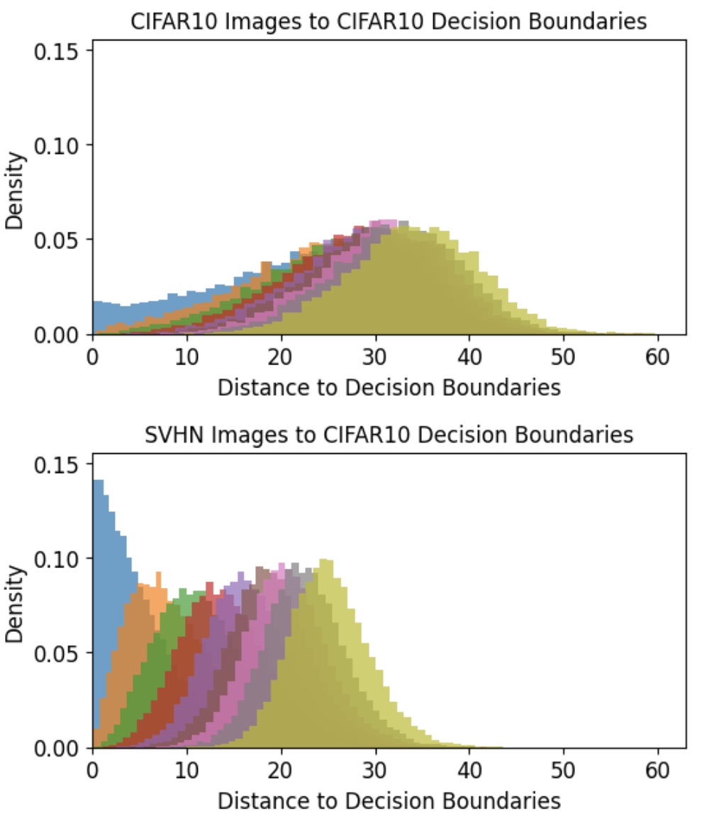
Figure 5: Individual Feature Distance to Decision Boundaries. ID features tend to be further from the decision boundaries than OOD features. Upper: ID feature distances to decision boundaries. Lower: OOD feature distances to decision boundaries. We sorted the distances measured for each sample in the plot.

12 Quantitative Study of the Proposed Distance Measuring method

In Section 3.1, we propose a closed-form estimation for measuring the feature distance to decision boundaries. To quantitatively understand the effectiveness and efficiency of our proposed method, we compare our method to iterative optimization for measuring the distance. In particular, we use targeted CW $L2$ attacks [1] on feature space which can effectively construct a targeted adversarial example under $L2$-distance from an iterative process. Empirically, CW attack based estimation and our closed-form estimation differs by $<1.5\%$. This implying the our closed-form estimation differs from the true value by $<1.5\%$, since estimation from successful CW-attacks uppers bounds the distance whereas our closed form estimation lower bounds the distance.

We follow the Pytorch implementation of CW attacks in [24]. In all our experiments, we follow the default parameters of initial constant 2, learning rate 0.005, max iteration 500, and binary search step 3. In all our experiments, CW-attack has a success rate close to $100\%$ And on a Tesla T4 GPU, estimating the distance using CW attack takes 992.2ms per image per class. In contrast, our proposed method incurs negligible overhead in inference, significantly reducing the computational cost of measuring the distance.

13 Ablation Under FPR95

In addition to the AUROC score reported in the main paper, we also compare the performance of OOD detection on ImageNet benchmarks using the regularized average distance $\mathtt{regDistDB}$, the regularization term $\|z-\mu_{train}\|_{2}$, as well as the un-regularized average distances $\mathtt{avgDistDB}$ as detection scores respectively. We report the performance of the detection scores in Table 6 under FPR95, the false positive rate of OOD samples when the ture positive rate of ID samples is at $95\%$. The results in FPR95 further validate the effectiveness of regularization in our OOD detector.

Table 6: Regularization enhances the effectiveness of OOD detection. FPR95 scores reported on ImageNet Benchmarks (lower is better). $\mathtt{regDistDB}$ outperforms $\mathtt{avgDistDB}$.

References

- Carlini and Wagner [2017] Nicholas Carlini and David Wagner. Towards evaluating the robustness of neural networks. In 2017 ieee symposium on security and privacy (sp), pages 39–57. Ieee, 2017.
- Cimpoi et al. [2014] Mircea Cimpoi, Subhransu Maji, Iasonas Kokkinos, Sammy Mohamed, and Andrea Vedaldi. Describing textures in the wild. In IEEE Conference in Computer Vision and Pattern Recognition, pages 3606–3613, 2014.
- Deng et al. [2009] Jia Deng, Wei Dong, Richard Socher, Li-Jia Li, Kai Li, and Li Fei-Fei. Imagenet: A large-scale hierarchical image database. In 2009 IEEE conference on computer vision and pattern recognition, pages 248–255. Ieee, 2009.
- DeVries and Taylor [2018] Terrance DeVries and Graham W Taylor. Learning confidence for out-of-distribution detection in neural networks. arXiv preprint arXiv:1802.04865, 2018.
- Djurisic et al. [2022] Andrija Djurisic, Nebojsa Bozanic, Arjun Ashok, and Rosanne Liu. Extremely simple activation shaping for out-of-distribution detection. arXiv preprint arXiv:2209.09858, 2022.
- Dosovitskiy et al. [2020] Alexey Dosovitskiy, Lucas Beyer, Alexander Kolesnikov, Dirk Weissenborn, Xiaohua Zhai, Thomas Unterthiner, Mostafa Dehghani, Matthias Minderer, Georg Heigold, Sylvain Gelly, et al. An image is worth 16x16 words: Transformers for image recognition at scale. arXiv preprint arXiv:2010.11929, 2020.
- Du et al. [2022] Xuefeng Du, Zhaoning Wang, Mu Cai, and Yixuan Li. Vos: Learning what you don’t know by virtual outlier synthesis. arXiv preprint arXiv:2202.01197, 2022.
- Fort et al. [2021] Stanislav Fort, Jie Ren, and Balaji Lakshminarayanan. Exploring the limits of out-of-distribution detection. Advances in Neural Information Processing Systems, 34:7068–7081, 2021.
- Hendrycks and Gimpel [2016] Dan Hendrycks and Kevin Gimpel. A baseline for detecting misclassified and out-of-distribution examples in neural networks. arXiv preprint arXiv:1610.02136, 2016.
- Hendrycks et al. [2019] Dan Hendrycks, Steven Basart, Mantas Mazeika, Mohammadreza Mostajabi, Jacob Steinhardt, and Dawn Song. Scaling out-of-distribution detection for real-world settings. arXiv preprint arXiv:1911.11132, 2019.
- Hsu et al. [2020] Yen-Chang Hsu, Yilin Shen, Hongxia Jin, and Zsolt Kira. Generalized odin: Detecting out-of-distribution image without learning from out-of-distribution data. In Proceedings of the IEEE/CVF Conference on Computer Vision and Pattern Recognition, pages 10951–10960, 2020.
- Huang et al. [2017] Gao Huang, Zhuang Liu, Laurens Van Der Maaten, and Kilian Q Weinberger. Densely connected convolutional networks. In Proceedings of the IEEE conference on computer vision and pattern recognition, pages 4700–4708, 2017.
- Huang and Li [2021] Rui Huang and Yixuan Li. Mos: Towards scaling out-of-distribution detection for large semantic space. In Proceedings of the IEEE/CVF Conference on Computer Vision and Pattern Recognition, pages 8710–8719, 2021.
- Huang et al. [2021] Rui Huang, Andrew Geng, and Yixuan Li. On the importance of gradients for detecting distributional shifts in the wild. Advances in Neural Information Processing Systems, 34:677–689, 2021.
- Khosla et al. [2020] Prannay Khosla, Piotr Teterwak, Chen Wang, Aaron Sarna, Yonglong Tian, Phillip Isola, Aaron Maschinot, Ce Liu, and Dilip Krishnan. Supervised contrastive learning. Advances in Neural Information Processing Systems, 33:18661–18673, 2020.
- Krizhevsky et al. [2009] Alex Krizhevsky, Geoffrey Hinton, et al. Learning multiple layers of features from tiny images. 2009.
- Lee et al. [2018] Kimin Lee, Kibok Lee, Honglak Lee, and Jinwoo Shin. A simple unified framework for detecting out-of-distribution samples and adversarial attacks. Advances in neural information processing systems, 31, 2018.
- Liang et al. [2018] Shiyu Liang, Yixuan Li, and R Srikant. Enhancing the reliability of out-of-distribution image detection in neural networks. In 6th International Conference on Learning Representations, ICLR 2018, 2018.
- Liu et al. [2020] Weitang Liu, Xiaoyun Wang, John Owens, and Yixuan Li. Energy-based out-of-distribution detection. Advances in Neural Information Processing Systems, 33:21464–21475, 2020.
- Loshchilov and Hutter [2016] Ilya Loshchilov and Frank Hutter. Sgdr: Stochastic gradient descent with warm restarts. arXiv preprint arXiv:1608.03983, 2016.
- Ming et al. [2022] Yifei Ming, Yiyou Sun, Ousmane Dia, and Yixuan Li. How to exploit hyperspherical embeddings for out-of-distribution detection? arXiv preprint arXiv:2203.04450, 2022.
- Ndiour et al. [2020] Ibrahima Ndiour, Nilesh Ahuja, and Omesh Tickoo. Out-of-distribution detection with subspace techniques and probabilistic modeling of features. arXiv preprint arXiv:2012.04250, 2020.
- Nguyen et al. [2015] Anh Nguyen, Jason Yosinski, and Jeff Clune. Deep neural networks are easily fooled: High confidence predictions for unrecognizable images. In Proceedings of the IEEE conference on computer vision and pattern recognition, pages 427–436, 2015.
- Papernot et al. [2018] Nicolas Papernot, Fartash Faghri, Nicholas Carlini, Ian Goodfellow, Reuben Feinman, Alexey Kurakin, Cihang Xie, Yash Sharma, Tom Brown, Aurko Roy, Alexander Matyasko, Vahid Behzadan, Karen Hambardzumyan, Zhishuai Zhang, Yi-Lin Juang, Zhi Li, Ryan Sheatsley, Abhibhav Garg, Jonathan Uesato, Willi Gierke, Yinpeng Dong, David Berthelot, Paul Hendricks, Jonas Rauber, and Rujun Long. Technical report on the cleverhans v2.1.0 adversarial examples library. arXiv preprint arXiv:1610.00768, 2018.
- Sehwag et al. [2020] Vikash Sehwag, Mung Chiang, and Prateek Mittal. Ssd: A unified framework for self-supervised outlier detection. In International Conference on Learning Representations, 2020.
- Sun and Li [2022] Yiyou Sun and Yixuan Li. Dice: Leveraging sparsification for out-of-distribution detection. In European Conference on Computer Vision, pages 691–708. Springer, 2022.
- Sun et al. [2021] Yiyou Sun, Chuan Guo, and Yixuan Li. React: Out-of-distribution detection with rectified activations. Advances in Neural Information Processing Systems, 34:144–157, 2021.
- Sun et al. [2022] Yiyou Sun, Yifei Ming, Xiaojin Zhu, and Yixuan Li. Out-of-distribution detection with deep nearest neighbors. arXiv preprint arXiv:2204.06507, 2022.
- Tack et al. [2020] Jihoon Tack, Sangwoo Mo, Jongheon Jeong, and Jinwoo Shin. Csi: Novelty detection via contrastive learning on distributionally shifted instances. Advances in neural information processing systems, 33:11839–11852, 2020.
- Tao et al. [2023] Leitian Tao, Xuefeng Du, Xiaojin Zhu, and Yixuan Li. Non-parametric outlier synthesis. arXiv preprint arXiv:2303.02966, 2023.
- Van Horn et al. [2018] Grant Van Horn, Oisin Mac Aodha, Yang Song, Yin Cui, Chen Sun, Alex Shepard, Hartwig Adam, Pietro Perona, and Serge Belongie. The inaturalist species classification and detection dataset. In Proceedings of the IEEE conference on computer vision and pattern recognition, pages 8769–8778, 2018.
- Wang et al. [2022] Haoqi Wang, Zhizhong Li, Litong Feng, and Wayne Zhang. Vim: Out-of-distribution with virtual-logit matching. In Proceedings of the IEEE/CVF conference on computer vision and pattern recognition, pages 4921–4930, 2022.
- Wei et al. [2022] Hongxin Wei, Renchunzi Xie, Hao Cheng, Lei Feng, Bo An, and Yixuan Li. Mitigating neural network overconfidence with logit normalization. arXiv preprint arXiv:2205.09310, 2022.
- Xiao et al. [2010] Jianxiong Xiao, James Hays, Krista A Ehinger, Aude Oliva, and Antonio Torralba. Sun database: Large-scale scene recognition from abbey to zoo. In 2010 IEEE computer society conference on computer vision and pattern recognition, pages 3485–3492. IEEE, 2010.
- Xu et al. [2015] Pingmei Xu, Krista A Ehinger, Yinda Zhang, Adam Finkelstein, Sanjeev R Kulkarni, and Jianxiong Xiao. Turkergaze: Crowdsourcing saliency with webcam based eye tracking. arXiv preprint arXiv:1504.06755, 2015.
- Yang et al. [2021] Jingkang Yang, Kaiyang Zhou, Yixuan Li, and Ziwei Liu. Generalized out-of-distribution detection: A survey. arXiv preprint arXiv:2110.11334, 2021.
- Yu et al. [2015] Fisher Yu, Ari Seff, Yinda Zhang, Shuran Song, Thomas Funkhouser, and Jianxiong Xiao. Lsun: Construction of a large-scale image dataset using deep learning with humans in the loop. arXiv preprint arXiv:1506.03365, 2015.
- Zhou et al. [2017] Bolei Zhou, Agata Lapedriza, Aditya Khosla, Aude Oliva, and Antonio Torralba. Places: A 10 million image database for scene recognition. IEEE transactions on pattern analysis and machine intelligence, 40(6):1452–1464, 2017.