Anomaly detection for automated inspection of power line insulators

Abstract

Inspection of insulators is important to ensure reliable operation of the power system. Deep learning has recently been explored to automate the inspection process by leveraging aerial images captured by drones along with powerful object detection models. However, a purely object detection-based approach exhibits class imbalance-induced poor detection accuracy for faulty insulators, especially for incipient faults. In order to address this issue in a data-efficient manner, this article proposes a two-stage approach that leverages object detection in conjunction with anomaly detection to reliably detect faults in insulators. The article adopts an explainable deep neural network-based one-class classifier for anomaly detection, that reduces the reliance on plentifully available images of faulty insulators, that might be difficult to obtain in real-life applications. The anomaly detection model is trained with two datasets – representing data abundant and data scarce scenarios – in unsupervised and semi-supervised manner. The results suggest that including as few as six real anomalies in the training dataset significantly improves the performance of the model, and enables reliable detection of rarely occurring faults in insulators. An analysis of the explanations provided by the anomaly detection model reveals that the model is able to accurately identify faulty regions on the insulator disks, while also exhibiting some false predictions.

[ETHZ]organization=Reliability and Risk Engineering, addressline=Department of Mechanical and Process Engineering, city=Zurich, postcode=8092, country=Switzerland

1 Introduction

Power transmission insulators play a key role in ensuring safe operation of the power system, and thus, power system operators conduct regular inspections of insulators, typically through on-site observations. The availability of high-quality images acquired with unmanned aerial surveillance vehicles has paved the way for advanced image processing techniques and deep learning models to be used for automated inspection of insulators. Recent literature shows an increasing interest in exploiting deep learning to automate the inspection of insulators.

Several machine learning-based and deep learning-based methods have been applied for inspection of power line insulators from aerial images. The authors in [1] adopted saliency maps obtained through static feature extraction, and segmented an insulator in an image. They combined local and global saliency maps, and identified insulators in complex backgrounds. On the other hand, [2] adopted an object detection-based approach, and trained a Faster Region proposal-based Convolutional Neural Network (Faster RCNN) model to detect three different types of insulators. In addition, the authors performed detection of missing caps of insulators, and achieved a fault detection precision of $92\%$. Similarly, [3] trained a Single-Shot multi-box Detector (SSD) model to detect healthy and faulty insulators, and obtained a precision of $92.48\%$. The authors in [4] modified the You Only Look Once version 2 (YOLOv2) model for insulator inspection, and obtained a detection precision of $94.2\%$ with one missing disk and $98.3\%$ with multiple missing disks in the insulators.

More recent model architectures that improve the robustness of detection performance have also been proposed in the literature. In [5], the authors coupled YOLOv3 with Dense-Blocks to enhance feature extraction. The experiments showed that the approach can detect insulators of different sizes and diverse backgrounds. The authors in [6] used a weakly supervised approach to count disks and find missing disks given only the bounding box of an insulator. The approach achieved competitive results with precision and recall of $92.86\%$ and $86.67\%$, respectively. A two-stage object detection approach was proposed in [7], where an object detector identifies the insulator position in the first stage, followed by a YOLOv3 model that identifies missing disks in the second stage. Similarly, [8] used different versions of YOLO, including v3, v4, and a coupling of Cross Stage Partial Network and YOLOv3. The results showed that the latter approach outperforms the other YOLO versions in identifying missing disks. A robust but efficient approach that employs lightweight CNN and channel attention mechanism was proposed in [9] to detect insulators and missing disks. This approach resulted in high accuracy and models with small size.

However, the above methods suffer from several drawbacks. The approach developed in [1] is limited to detection of insulators, and cannot differentiate between healthy and faulty ones. Many object detection-based methods are developed with small datasets (e.g., $80$ images for training and $40$ images for testing [2], $385$ images for training and $100$ images for testing [4], 573 images for training and 191 images for testing [7]), with little or no investigation of the sensitivity to image features in the background and foreground. In addition, the fault detection methods discussed above address the relatively simpler task of detecting missing caps/disks, and ignore finer faults such as flashed and broken disks [10]. The flash-over caused by electrical flashes or lightning strikes and irregularly shaped broken disks are important for the operator’s situational awareness and informed prioritisation of maintenance activities. The authors in [10] have targeted this gap, and have studied the performance of object detection models for these finer faults. They compared four models with two datasets, and showed that YOLOv5 performs the best in data-abundant and data-scarce scenarios. The authors further identified class imbalance and size imbalance as major challenges impeding the detection of smaller and infrequently observed objects, i.e., flashed and broken disks. Thus, while object detection models are capable of simultaneously detecting multiple objects in an image, their performance is still limited by the volume of available data. This poses a challenge to automating the inspection process for a well-functioning grid, since the vast majority of insulators will be healthy. Thus, this challenge cannot be tackled through the collection of more images and requires methodological improvement. In this article, we address the shortcomings of a purely detection-based strategy, and adopt a two-stage approach that relies on both detection and segmentation to deliver a significant improvement in identifying infrequent objects, i.e., flashed and broken disks.

1.1 Contributions

This article makes the following contributions:

1. We pose the detection of flashed and broken disks as an anomaly detection problem and adopt a state-of-the-art explainable one-class classification-based anomaly detector. This model takes images of disks as input, which can be generated beforehand by an object detection model.

2. We study the performance of this approach with two datasets of different sizes, i.e., in data-abundant and data-scarce scenarios.

3. We leverage data from both datasets to improve the performance of the model in the data scarce scenario.

The rest of the article is organized as follows: Section 2 presents the methodology adopted in this work. Section 3 presents the application of the anomaly detection model to insulator fault detection along with the dataset collection and curation procedure. The experimental setup is also discussed in Section 3. Section 4 presents the results of our experiments. Finally, Section 5 provides concluding remarks.

2 Methodology

In this section, we discuss our motivation to adopt an anomaly detection-based approach to solve the fault detection problem for insulators. This is followed by a description of the state-of-the-art one-class classification-based approach adopted in this work for building an anomaly detector, i.e., fully convolutional data description [11].

2.1 Insulator fault detection as an anomaly detection problem

We address the problem of insulator fault detection, i.e., identifying the presence of faults in insulators. We consider two types of faults, i.e., flashed disks and broken disks, which have not been extensively studied in the literature. In a recent work, this problem has proved elusive with an object detection-based approach in data-scarce scenarios [10]. Specifically, state-of-the-art object detection models perform very well for detecting insulators (which have high frequency and large size), relatively poorer for healthy disks (very high frequency but small size) and very poor for flashed disks (very low frequency and small size) [10]. As discussed above, the challenge of class imbalance cannot be addressed by collecting more images. Further, size imbalance is inherent to the application, and cannot be avoided. This motivates the need for a methodologically different approach that can reliably differentiate between healthy and faulty disks. To that end, we investigate the source of poor performance for the flashed disks, and observe that classification errors are the primary contributor to the poor performance, rather than localisation errors. This implies that the object detection models are capable of accurately localising disks and only encounter difficulty in correctly distinguishing between the healthy and faulty ones. This naturally leads us to investigate whether a second model dedicated to classify healthy and faulty disks can benefit the fault detection task. In this work, we adopt a two-stage approach that utilizes two models. The first model is an object detector that localizes insulators and disks, and the second model is an anomaly detector that performs fault detection on the extracted disks. Finally, a deterministic post-processing step can identify unhealthy insulators by mapping flashed and broken disks to their source insulators. This approach is presented in Figure 1.

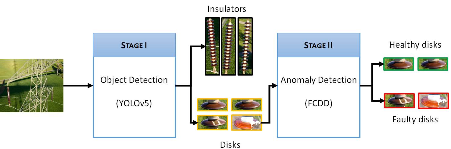
Figure 1: Two-stage insulator fault detection with object detection and anomaly detection. The texts in parentheses represent the particular type of model used in this work.

A two-stage approach divides the fault detection task, and thus, makes it easier for the individual models to perform better. Specifically, in the first stage, a 2-class object detection model will suffice, as opposed to a 4-class model in purely object detection-based approach. In the second stage, since the samples consist of only extracted images of accurately localised disks, one has to deal with very little background compared to the first stage. This is evident from Figure 2, which shows sample aerial images of insulators, and extracted images of disks. As a result, one can expect that the two-stage approach will perform better than a one-stage approach.

(a) Aerial images of insulators

(b) Extracted images of disks

Figure 2: Aerial images of insulators and extracted images of disks. The extracted images contain very little background compared to aerial images.

The first stage of the proposed approach involves training a reliable object detection model for localisation of insulators and disks, which has already been performed in [10]. Therefore, in this work, we focus only on developing the second stage and building a model that can differentiate between different types of disks. This stage will use only images of disks, and will thus be free from size imbalance. However, class imbalance between healthy and faulty disks still persists, and needs to be carefully addressed. The problem associated with the second stage is to detect faulty disks, which occur very infrequently in a dataset with a large number of healthy disks. This naturally lends itself as an anomaly detection problem. Anomaly detection aims at detecting rarely occurring data points (anomalies) that deviate significantly from very frequently observed normal data points [12]. Anomaly detection is used in several applications such as blockchain networks [13], financial fraud detection [14] and time series analysis [15]. This approach is also adopted for fault detection in marine engineering [16], robotics [17], electrical engineering [18], autonomous driving [19] and photovoltaics [20].

There are several approaches for anomaly detection for different types of data [21]. In this work, we are interested in anomaly detection with images of disks, and thus, adopt a deep learning-based approach to address this problem. A detailed taxonomy and review of the algorithms for anomaly detection using deep learning is presented in [22]. Deep learning-based methods often adopt autoencoders for image [23] and video [24] anomaly detection, which are trained on normal data points. Since such a model only sees normal data points during training, it is expected to exhibit high errors in reconstructing an anomalous data point, thereby allowing anomaly detection by monitoring the reconstruction error of the model. While such models are very popular, they do not offer a way to include any prior information about anomalies during training. However, in the case of detecting faulty disks, one has prior information about the flash-over patterns and shapes of broken disks, that could be leveraged to improve the performance of the model. We therefore employ a state-of-the-art anomaly detection method that allows one to use the patterns observed in anomalous data points during training. In addition, the model can also provide explanations for its predictions, which can benefit its adoption by the industry.

2.2 Anomaly detection with fully convolutional data description

The fully convolutional data description (FCDD) is a state-of-the-art anomaly detection approach [11] that has been demonstrated to provide excellent performance on standard datasets, including ImageNet and MVTec-AD, which is a dataset for detecting defects in manufacturing [25]. FCDD is a one-class classification model, that performs anomaly detection by mapping all normal data points in the vicinity of a centre $\mathbf{c}$ in the output space, which results in the anomalies being mapped away from $\mathbf{c}$. FCDD is based on the hypersphere classifier, which employs the following loss function:

$$\begin{split}\mathcal{L}_{HSC}=\frac{1}{N}\sum_{i=1}^{N}&\Big{[}\left(1-y_{i}\right)\tilde{h}\left(f\left(x_{i};\theta\right)-\mathbf{c}\right)\\ &-y_{i}\log\left(1-\exp\left(-\tilde{h}\left(f\left(x_{i};\theta\right)-\mathbf{c}\right)\right)\right)\Big{]}\end{split}$$ (1)

where, $x_{i}\in\mathbb{R}^{c\times h\times w}$ represents the $i^{th}$ input, $y_{i}\in\{1,0\}$ represents the $i^{th}$ target such that $y_{i}=1$ for anomalous data points, and $y_{i}=0$ for normal data points, $N$ represents the number of data points, $f(\cdot;\theta)$ represents the neural network parameterised in $\theta$, and $\tilde{h}(\cdot)$ represents the pseudo-Huber loss, defined as: $\tilde{h}(x)=\sqrt{||x||_{2}^{2}+1}-1$. FCDD uses a fully convolutional architecture for the neural network $f(\cdot;\theta)$, which transforms the input $x_{i}\in\mathbb{R}^{c\times h\times w}$ to feature $z_{i}\in\mathbb{R}^{u\times v}$. In addition, the centre of the hypersphere is set to the bias of the last layer of $f$, so that the FCDD loss can be expressed as:

$$\begin{split}\mathcal{L}_{FCDD}=\frac{1}{N}\sum_{i=1}^{N}&\Bigg{[}\left(1-y_{i}\right)\frac{1}{u\cdot v}||\tilde{h}\left(z_{i}\right)||_{1}\\ &-y_{i}\log\left(1-\exp\left(-\frac{1}{u\cdot v}||\tilde{h}\left(z_{i}\right)||_{1}\right)\right)\Bigg{]}.\end{split}$$ (2)

The quantity $\tilde{h}(z_{i})$ is the pseudo-Huber loss of the features. This loss is summed for all entries of $\tilde{h}(z_{i})$, and then normalised with respect to the number of entries, which provides a normalised measure of deviation of the feature from the centre. The above objective minimises the deviation for normal data points ($y_{i}=0$), and maximises the deviation for anomalous data points ($y_{i}=1$). The features of a trained FCDD model can be considered as a heatmap of the input, with anomalous regions exhibiting higher values, and normal regions exhibiting lower values. In general, the dimension of the features is lower compared to that of the input of a convolutional network, i.e., here $u<h,v<w$. In order to map this low-resolution heatmap to the original input image, FCDD further performs a deterministic upsampling of $z$ with a Gaussian kernel [11].

In the above formulation, the model takes only the images and labels, i.e., normal or anomalous, and learns a mapping that highlights the anomalous regions of an image. When anomalous images are used for training in this setting, information about patterns observed in faulty images is implicitly provided to the model. It is also possible to explicitly incorporate prior knowledge at the time of training, which can be achieved by modifying the FCDD loss to allow semi-supervised training as follows [11]:

$$\begin{split}\mathcal{L}_{FCDD}^{SS}=\frac{1}{N}\sum_{i=1}^{N}&\left[\frac{1}{w\cdot h}\sum_{j=1}^{w\cdot h}\left(1-y_{i,j}\right)\tilde{z}_{i,j}\right.\\ &\left.-\log\left(1-\exp\left(-\frac{1}{w\cdot h}\sum_{j=1}^{w\cdot h}y_{i,j}\tilde{z}_{i,j}\right)\right)\vphantom{\frac{1}{1\cdot h}}\right]\end{split}$$ (3)

where, $y_{i}\in\{1,0\}^{h\times w}$ is the ground truth map for the $i^{th}$ image, and contains $1$ for all pixels exhibiting an anomaly, and $\tilde{z}\in\mathbb{R}^{h\times w}$ represents the up-sampled features. The above loss function has been shown to result in better performing models [11].

3 Insulator fault detection with FCDD

In this work, we use FCDD in both formulations (Eqs. (2) and (3)) to differentiate between healthy and faulty disks. In the first formulation, it is possible to learn from only normal samples, i.e., without including any anomalies at the time of training. It is also possible to use images of any object other than disks as anomalous samples, or employ an outlier exposure algorithm to synthetically generate anomalies, both of which improve the performance of the model [11]. Finally, it is possible to include real anomalies (without any ground truth anomaly maps) to minimise $\mathcal{L}_{FCDD}$. In all of these scenarios, either no real anomalies are used at the time of training, or the ground truth anomaly maps of real anomalies are not provided, resulting in unsupervised training. We perform unsupervised training with (i) no faulty disks and (ii) real faulty disks without anomaly maps. In addition, we also perform semi-supervised training by minimising $\mathcal{L}_{FCDD}^{SS}$, wherein we provide the ground truth anomaly masks during training.

3.1 Dataset preparation

We investigate the performance of FCDD with two datasets. The first dataset is an openly available dataset curated by the Electric Power Research Institute and is referred to as the Insulator Defect Image Dataset (IDID) [26]. This dataset consists of $1600$ images of insulators with a variety of disks colours. Each image in this dataset has four orientations – original, diagonally flipped, horizontally flipped and vertically flipped. In this work, we use only the images with original orientations, which results in $400$ images with $3286$ healthy disks, $716$ flashed disks and $282$ broken disks. This dataset is used to study the performance of anomaly detection in data-abundant scenario. The second dataset (referred to as SG) is a collection of $77$ aerial images collected by Swissgrid AG, with $2429$ healthy disks, only $53$ flashed disks and no broken disks. This dataset is used as the data-scarce scenario in this study. Since semi-supervised training requires the ground truth anomaly maps, these datasets are manually labelled with the “labelme” tool [27]. This involves generating polygonal segmentation masks for flash-over patches and regions of broken disks. The segmentation masks are then converted to $\{0,1\}^{h\times w}$ to obtain the ground truth map, which are shown in Figure 3 for healthy, flashed and broken disks. Note that the maps for healthy disks are completely black, and can be generated automatically. This reduces the manual burden of labelling only faulty disks.

(a) Healthy disk and its map

(b) Flashed disk and its map

(c) Broken disk and its map

Figure 3: Sample disks (healthy, flashed and broken), and their corresponding ground truth maps for semi-supervised training.

3.2 Experimental setup

We first study the performance of the FCDD model trained individually on IDID and SG datasets and compare the performance in data-abundant (Section 4.1) and data-scarce (Section 4.2) scenarios. Then, we investigate whether data from a different dataset can be used to improve the performance in a data-scarce scenario (Section 4.3). To that end, we include data from both IDID and SG datasets to train a third FCDD model and examine if it performs better compared to the model trained only on SG dataset. Note that while IDID has two types of faulty disks (flashed and broken), the SG dataset has only flashed disks. Thus, we train an FCDD model for the IDID dataset with both types of faulty disks for IDID, and use only flashed disks of IDID to augment the performance of (the third) FCDD for the SG dataset. The number of training and testing images used for different experiments are listed in Table 1. As an illustrative case, for unsupervised training with no real anomalies for IDID, we use $2586$ healthy disks, while for semi-supervised training, we additionally use $200$ faulty disks and $100$ broken disks.

Dataset	#Healthy Samples		#Anomalous Samples
	Train	Test	Train	Test
SG	2379	50	6	47
IDID	2586	700	200 (F)	516 (F)
			+ 100 (B)	+ 182 (B)
SG	2379	50	6	47
+ IDID	0	0	716	0

Table 1: Number of samples used for training and testing of FCDD for insulator fault detection. In unsupervised training, we use all healthy samples along with 1) no anomalous samples or 2) anomalous samples without ground truth maps. In semi-supervised training, we utilize all healthy and anomalous samples with the ground truth maps. ((F): Flashed disks, (B): Broken disks).

All experiments are performed with the FCDD package [11]. The default settings of FCDD have been employed, of which the notable settings are an input image size of $3\times 224\times 224$, the VGG-11-BN-based deep convolutional model [28], a batch size of $128$, $200$ epochs for training and stochastic gradient descent optimizer. All experiments are performed on a Windows workstation with one NVIDIA RTX $3070$ GPU and $128$ GB of RAM. In order to evaluate and compare the performance of the models, we employ the standard area under the receiver operating characteristics curve (AUC) metric. The AUC can be expressed as:

$$AUC=\int\limits_{\mathcal{T}}R_{TP}dR_{FP},$$ (4)

where $R_{TP}$ and $R_{FP}$ are the true positive rate and false positive rate, respectively, and are obtained as:

$$R_{TP} = \frac{\text{TP}}{\text{TP}+\text{FN}}$$

$$R_{FP} = \frac{\text{FP}}{\text{FP}+\text{TN}}$$

where, TP, TN, FP and FN represent true positives, true negatives, false positives and false negatives, respectively. $\mathcal{T}$ represents the set of all decision thresholds used to predict the positives and negatives. First, different values of true and false positive rates are obtained for different classification thresholds, and AUC is then calculated according to Equation 4. The optimal decision threshold can be obtained from the receiver operating characteristics by identifying the top-left point of the curve, which can then be used to evaluate the classification accuracy of the model. In order to account for uncertainty during training, FCDD trains $5$ different instances of a model by default. We report the average performance (AUC and optimal accuracy) of the five models in each experiment.

4 Results

In this section, we present an evaluation and comparison of FCDD models trained for data-abundant and data-scarce scenarios, with different formulations. We then present the explanations provided by the semi-supervised FCDD model for its predictions, followed by a discussion of the results and future work.

4.1 Fault detection with data abundance

Unsupervised training of the FCDD model without any faulty samples provides an AUC of $0.5923$ for IDID, corresponding to a classification accuracy of $0.5735$ for the optimal decision threshold. The AUC and optimal accuracy increase to $0.7920$ and $0.7172$, respectively with the inclusion of only flashed disks as anomalous data points during unsupervised training, i.e., without any ground truth anomaly maps. This is a large improvement in performance, achieved with only $200$ training images of flashed disks, and underscores the significance of using real anomalies at the time of training. We also trained models with both broken and flashed disks (without any ground truth anomaly maps), and observed the AUC to be $0.7491$, corresponding to an accuracy of $0.6889$. This further demonstrates that FCDD can learn from multiple types of anomalies in the training dataset, and deliver performance comparable with learning from only one type of anomaly.

In the semi-supervised formulation, the FCDD model provides an AUC of $0.9091$, and an accuracy of $0.8292$, when trained and tested with only flashed disks as anomalous data points. This demonstrates the advantage of using ground truth anomaly maps to inform the training process about the patterns observed in faulty data – in a more explicit manner. Similar to the unsupervised formulation, we performed semi-supervised training with both broken and flashed disks, and obtained an AUC of $0.9040$, corresponding to an accuracy of $0.8266$. This again demonstrates the capability of the FCDD model to deliver comparable performance with multiple types of anomalies. It must be noted, however, that the model can only differentiate between normal (healthy) and anomalous (faulty) data points, and cannot identify the nature of an anomaly (flashed or broken).

4.2 Fault detection with data scarcity

In the data-scarce application, the unsupervised FCDD model trained without any real anomalies provides an AUC of $0.7387$ and an accuracy of $0.7051$, which is considerably higher than the performance in data data-abundant scenario. This difference may partly be attributed to the larger number of images used to evaluate the models in data-abundant scenario, which exposes the model to more variations in the images. The model trained with flashed disks as anomalies provides an AUC of $0.8495$ and an accuracy of $0.7608$. This suggests that FCDD can leverage information about the anomalies in an efficient manner, i.e., with only $6$ anomalies, and provide a considerable improvement in the performance of fault detection.

In the semi-supervised formulation, the FCDD model delivers an AUC of $0.8830$, corresponding to an optimal accuracy of $0.8061$. This further highlights the value of using ground truth anomaly maps to inform the training process about the specific patterns of faults.

4.3 Improving anomaly detection in data scarce scenario

We adopt two different methods of increasing the training dataset size to improve the performance in data-scarce scenario. In the first approach, we increase the number of training anomalies to cover half of the total number of available anomalies. We perform this experiment in both the unsupervised and semi-supervised settings. The AUCs of the models trained with $6$, $14$, $20$ and $26$ anomalies are shown in Figure 4. The AUC of the unsupervised model without any training anomalies is also shown for reference. We observe that both models provide a consistent improvement in performance with more training anomalies. The semi-supervised models can also be seen to perform better than the unsupervised models for all the cases. The model trained with $26$ anomalies provides an AUC of $0.9193$ and an optimal accuracy of $0.8337$ with unsupervised training. The corresponding semi-supervised model provides an AUC of $0.9363$ and an accuracy of $0.8597$.

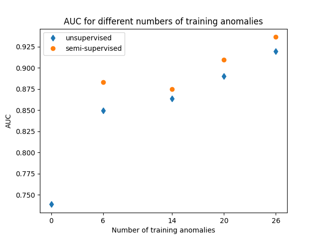
Figure 4: AUC of FCDD models trained on SG dataset with different numbers of training anomalies.

In the above approach, the number of anomalies used for testing the model is different across the scenarios. In order to maintain the same test images, and increase the number of training anomalies, we further leverage data from IDID. Specifically, we use all images of flashed disks in IDID, in addition to the $6$ training anomalies, and train unsupervised and semi-supervised FCDD models. The unsupervised model provides an AUC of $0.7940$ with an accuracy of $0.7237$, which is poorer than the corresponding model trained with only $6$ anomalies of SG dataset. The semi-supervised model provides an AUC of $0.8860$ and an accuracy of $0.8123$, which is only marginally better than the corresponding model trained with only SG dataset. These observations suggest that in an unsupervised formulation, including training anomalies from a different dataset hampers the learning process, while in the semi-supervised formulation, the advantage gained from such anomalies is minimal. Moreover, we observe that the patterns of flash-over of disks are similar for both datasets, suggesting that the poor performance might be partly due to the high variation of colours in disks of IDID, compared to the SG dataset.

4.4 Explanations of FCDD

The explanations from an FCDD model are obtained by up-sampling the model’s output features ($z$) to match the original image size, through a deterministic non-trainable Gaussian kernel-based approach [11]. The up-sampled features ($\tilde{z}$) are then represented as a heat map to highlight the anomalous regions predicted by the model. Figure 5 shows the explanations of the semi-supervised models on sample test images for both datasets. For each dataset, Figure 5 shows six sample test images (healthy in the left panel and faulty in the right panel), their explanations produced by the model, and the corresponding ground truth anomaly maps. It can be observed that the explanations for the faulty images match closely with the ground truth anomaly maps for the images from IDID. This suggests that the model is able to localise patches of discolouration on the disks with very good accuracy. The model also predicts anomalous regions on the disks that are not aligned with the ground truth anomaly maps. The explanations for the healthy images, on the other hand, consistently contain anomalous regions predicted by the model.

The explanations for the faulty images of the SG dataset are also well aligned with the ground truth maps, although they exhibit slightly more deviation from the ground truth anomaly maps compared to IDID. This can also be observed for the healthy images in this dataset. The qualitatively poor explanations for the SG dataset compared to IDID can be corroborated by the difference in AUC and optimal accuracy of the two models trained with these datasets. Although both models make false predictions, i.e., spurious anomalous regions (on disks, as well as in the background), these predictions are aggregated to decide whether the image is normal or anomalous. This aggregation and classification based on the optimal threshold finally provides a very good accuracy.

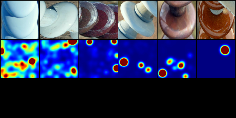
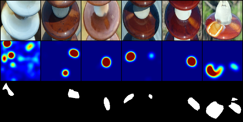
(a) Explanations for IDID (left: healthy, right: faulty).

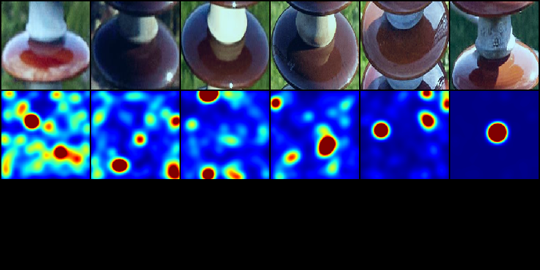
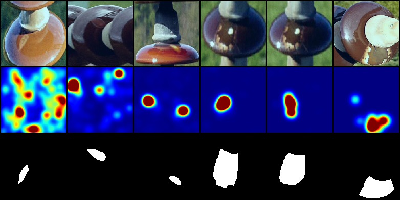
(b) Explanations for SG dataset (left: healthy, right: faulty).

Figure 5: Explanations of FCDD models for IDID (data abundant) and SG dataset (data scarce), trained in a semi-supervised manner. In each panel, the top, middle and bottom rows show the original image, explanations provided by the FCDD model and ground truth anomaly maps, respectively. The explanations are shown as heat maps, with higher values (shown in red) representing a faulty pattern and lower values (shown in blue) representing healthy pattern.

4.5 Discussion and future work

The two-stage approach proposed in this work merges object detection with anomaly detection to identify rarely occurring faults in insulators. At the time of deployment, the predictions from the object detection model can be used as input to the anomaly detection model. However, at the time of training, the parameters of the two models are learnt independently, i.e., without any shared parameters. Since the first stage aims at detecting insulators and disks, the model in the second stage (that deals with detecting patterns on disks) can potentially benefit from the learnt parameters of the object detection model. Such a study has not been conducted in this work, and can be explored in the future to potentially improve the performance and/or reduce the training time of the anomaly detection model.

We observed that including the faulty images from IDID did not provide a significant improvement in performance for the SG dataset. This could potentially be due to domain shift, which has not been investigated in this work. Future studies can also be directed towards incorporating methods of domain adaptation in the anomaly detection stage to improve the performance in data-scarce applications.

One of the biggest strengths of FCDD is the explainability of the model in terms of the predictions of faulty regions in the images. However, we observed that the explanations produced by the FCDD models, although highly accurate for several samples, can provide false predictions of faulty regions in some examples. Moreover, these false predictions can be on the disk, or in the background of the image. Improving the predictions of the FCDD models by, for example, adapting the loss function to penalise false positives, can be studied in the future. This will improve interpretability of the model, and facilitate the adoption of such a transparent model by the industry.

5 Conclusion

In this work, we proposed a two-stage approach that uses object detection and anomaly detection to reliably identify faults in insulators. A deep neural network-based explainable one-class classifier, i.e., fully convolutional data description (FCDD) was adopted to perform anomaly detection. FCDD allowed both unsupervised and semi-supervised training, which enabled informing the training process about the nature of faults observed in real anomalies. The model was trained with two datasets, representing data-abundant and data-scarce scenarios. The FCDD model provided very good performance, with AUCs of up to $0.9$ for the data-abundant application and $0.88$ for the data-scarce application. The semi-supervised model was observed to perform better than the unsupervised model for both datasets, which highlighted the value of providing real anomalies and ground truth anomaly maps at the time of training. However, the number of such anomalies is only $200$ for the data-abundant case and $6$ for the data-scarce case, which does not lead to a large labelling requirement for training the model.

The proposed approach provides a method to detect rarely occurring incipient faults, specifically flashed and broken disks in both data-abundant and data-scarce applications with minimal labelling efforts. The explanations of the model were also seen to match with the ground truth for many samples, with few false positive predictions. Improving the explanations of the model and accounting for domain shift are some of the open questions that can be addressed in the future.

References

- [1] L. Junfeng, L. Min, W. Qinruo, A novel insulator detection method for aerial images, in: Proceedings of the 9th International Conference on Computer and Automation Engineering, 2017, pp. 141–144.
- [2] X. Liu, H. Jiang, J. Chen, J. Chen, S. Zhuang, X. Miao, Insulator detection in aerial images based on faster regions with convolutional neural network, in: 2018 IEEE 14th International Conference on Control and Automation (ICCA), IEEE, 2018, pp. 1082–1086.
- [3] H. Jiang, X. Qiu, J. Chen, X. Liu, X. Miao, S. Zhuang, Insulator fault detection in aerial images based on ensemble learning with multi-level perception, IEEE Access 7 (2019) 61797–61810.
- [4] J. Han, Z. Yang, Q. Zhang, C. Chen, H. Li, S. Lai, G. Hu, C. Xu, H. Xu, D. Wang, et al., A method of insulator faults detection in aerial images for high-voltage transmission lines inspection, Applied Sciences 9 (10) (2019) 2009.
- [5] C. Liu, Y. Wu, J. Liu, Z. Sun, Improved yolov3 network for insulator detection in aerial images with diverse background interference, Electronics 10 (7) (2021) 771.
- [6] C. Shi, Y. Huang, Cap-count guided weakly supervised insulator cap missing detection in aerial images, IEEE Sensors Journal 21 (1) (2020) 685–691.
- [7] J. Han, Z. Yang, H. Xu, G. Hu, C. Zhang, H. Li, S. Lai, H. Zeng, Search like an eagle: A cascaded model for insulator missing faults detection in aerial images, Energies 13 (3) (2020) 713.
- [8] C. Liu, Y. Wu, J. Liu, Z. Sun, H. Xu, Insulator faults detection in aerial images from high-voltage transmission lines based on deep learning model, Applied Sciences 11 (10) (2021) 4647.
- [9] H. Xia, B. Yang, Y. Li, B. Wang, An improved centernet model for insulator defect detection using aerial imagery, Sensors 22 (8) (2022) 2850.
- [10] L. Das, M. H. Saadat, B. Gjorgiev, E. Auger, G. Sansavini, Object detection-based inspection of power line insulators: Incipient fault detection in the low data-regime (2022). arXiv:2212.11017.
-
[11]
P. Liznerski, L. Ruff, R. A. Vandermeulen, B. J. Franks, M. Kloft, K. R.
Muller, Explainable deep
one-class classification, in: International Conference on Learning
Representations, 2021.
URL https://openreview.net/forum?id=A5VV3UyIQz - [12] G. Pang, C. Shen, L. Cao, A. V. D. Hengel, Deep learning for anomaly detection: A review, ACM computing surveys (CSUR) 54 (2) (2021) 1–38.
- [13] M. U. Hassan, M. H. Rehmani, J. Chen, Anomaly detection in blockchain networks: A comprehensive survey, IEEE Communications Surveys & Tutorials (2022).
- [14] W. Hilal, S. A. Gadsden, J. Yawney, Financial fraud:: A review of anomaly detection techniques and recent advances (2022).
- [15] S. Schmidl, P. Wenig, T. Papenbrock, Anomaly detection in time series: a comprehensive evaluation, Proceedings of the VLDB Endowment 15 (9) (2022) 1779–1797.
- [16] C. Velasco-Gallego, I. Lazakis, Radis: A real-time anomaly detection intelligent system for fault diagnosis of marine machinery, Expert Systems with Applications 204 (2022) 117634.
- [17] T. Schnell, K. Bott, L. Puck, T. Buettner, A. Roennau, R. Dillmann, Robigan: A bidirectional wasserstein gan approach for online robot fault diagnosis via internal anomaly detection, in: 2022 IEEE/RSJ International Conference on Intelligent Robots and Systems (IROS), IEEE, 2022, pp. 4332–4337.
- [18] Y. Chen, Z. Zhao, H. Wu, X. Chen, Q. Xiao, Y. Yu, Fault anomaly detection of synchronous machine winding based on isolation forest and impulse frequency response analysis, Measurement 188 (2022) 110531.
- [19] Y. Fang, H. Min, X. Wu, X. Lei, S. Chen, R. Teixeira, X. Zhao, Toward interpretability in fault diagnosis for autonomous vehicles: Interpretation of sensor data anomalies, IEEE Sensors Journal (2023).
- [20] C. Li, Y. Yang, K. Zhang, C. Zhu, H. Wei, A fast mppt-based anomaly detection and accurate fault diagnosis technique for pv arrays, Energy Conversion and Management 234 (2021) 113950.
- [21] L. Ruff, J. R. Kauffmann, R. A. Vandermeulen, G. Montavon, W. Samek, M. Kloft, T. G. Dietterich, K.-R. Müller, A unifying review of deep and shallow anomaly detection, Proceedings of the IEEE 109 (5) (2021) 756–795.
- [22] J. Li, D. Yan, K. Luan, Z. Li, H. Liang, Deep learning-based bird’s nest detection on transmission lines using uav imagery, Applied Sciences 10 (18) (2020) 6147.
- [23] C. Zhou, R. C. Paffenroth, Anomaly detection with robust deep autoencoders, in: Proceedings of the 23rd ACM SIGKDD international conference on knowledge discovery and data mining, 2017, pp. 665–674.
- [24] Y. Zhao, B. Deng, C. Shen, Y. Liu, H. Lu, X.-S. Hua, Spatio-temporal autoencoder for video anomaly detection, in: Proceedings of the 25th ACM international conference on Multimedia, 2017, pp. 1933–1941.
- [25] P. Bergmann, M. Fauser, D. Sattlegger, C. Steger, Mvtec ad–a comprehensive real-world dataset for unsupervised anomaly detection, in: Proceedings of the IEEE/CVF conference on computer vision and pattern recognition, 2019, pp. 9592–9600.
- [26] P. Kulkarni, T. Shaw, D. Lewis, Insulator defect image dataset - version 1.2: Documentation EPRI, Palo Alto, CA: 2020. 3002017949.
-
[27]
K. Wada, Labelme: Image Polygonal
Annotation with Python.
doi:10.5281/zenodo.5711226.
URL https://github.com/wkentaro/labelme - [28] K. Simonyan, A. Zisserman, Very deep convolutional networks for large-scale image recognition (2015). arXiv:1409.1556.