Pinning, diffusive fluctuations, and Gaussian limits
for half-space directed polymer models

Abstract.

Half-space directed polymers in random environments are models of interface growth in the presence of an attractive hard wall. They arise naturally in the study of wetting and entropic repulsion phenomena. [Kar85] predicted a “depinning” phase transition as the attractive force of the wall is weakened. This phase transition has been rigorously established for integrable models of half-space last passage percolation, i.e. half-space directed polymers at zero temperature, in a line of study tracing back to the works [BR01, BR01a, BR01b]. On the other hand, for integrable positive temperature models, the first rigorous proof of this phase transition has only been obtained very recently through a series of works [BW23, IMS22, BCD23, DZ23] on the half-space log-Gamma polymer. In this paper we study a broad class of half-space directed polymer models with minimal assumptions on the random environment. We prove that an attractive force on the wall strong enough to macroscopically increase the free energy induces phenomena characteristic of the subcritical “bound phase,” namely the pinning of the polymer to the wall and the diffusive fluctuations and limiting Gaussianity of the free energy. Our arguments are geometric in nature and allow us to analyze the positive temperature and zero temperature models simultaneously. Moreover, given the macroscopic free energy increase proved in [IMS22] for the half-space log-Gamma polymer, our arguments can be used to reprove the results of [IMS22, DZ23] on polymer geometry and free energy fluctuations in the bound phase.

1. Introduction, main results, and proof ideas

Directed polymers in random environments, introduced in [HH85, IS88, Bol89], are a well-studied family of models in mathematical physics. The full-space directed polymer is widely believed to belong to the KPZ universality class. We refer the reader to the books [Gia07, Hol09, Com17] for further background on directed polymers.

Half-space directed polymers in random environments were introduced by Kardar [Kar85] as a natural model for wetting and entropic repulsion phenomena that occur as an interface grows in the presence of an attractive hard wall [Abr80, BHL83, PSW82]. Kardar predicted a “depinning” phase transition as the attractive force of the wall is weakened: in the subcritical or “bound” phase, the polymer is “pinned” to the wall; in the supercritical or “unbound” phase, the polymer is entropically repulsed away from the wall.

This phase transition was first rigorously established for geometric and Poissonian half-space last passage percolation (LPP), two integrable zero temperature half-space directed polymer models, by Baik–Rains [BR01, BR01a, BR01b]. They proved that the last passage time (i.e. zero temperature free energy) exhibits Gaussian statistics in the bound phase and KPZ universality class statistics in the critical and unbound phases. Analogous results were later obtained for exponential half-space LPP by Baik–Barraquand–Corwin–Suidan [BBCS18, BBCS18a].

A recent flurry of activity has led to a comparable mathematical understanding of the depinning phase transition for integrable positive temperature half-space polymer models. We only mention a handful of works in the following paragraph (also in the preceding paragraph), and we encourage the reader to consult [BCD23, Section 1.4] for a far more comprehensive review of the literature on this phase transition in integrable half-space models.

The depinning phase transition for the point-to-line half-space log-Gamma (HSLG) polymer has recently been proved by Barraquand–Wang [BW23], and for the point-to-point HSLG polymer by Imamura–Mucciconi–Sasamoto [IMS22]. Very recently Barraquand–Corwin–Das [BCD23] extended the results of [IMS22] on the HSLG polymer in the unbound phase, and moreover established the KPZ exponents ($1/3$ for the free energy fluctuations, $2/3$ for the transversal correlation length) in the critical and supercritical regimes. The main technical contribution of [BCD23] is the construction of the HSLG line ensemble, a Gibbsian ensemble of half-infinite lines whose top line is the point-to-point HSLG polymer free energy. In [DZ23], Das–Zhu applied the Gibbs property (invariance under local resampling) of the HSLG line ensemble to confirm the predicted pinning of the HSLG polymer to the wall in the bound phase. Specifically, [DZ23] proved that the endpoint of the point-to-line HSLG polymer typically lies within an $O(1)$-neighborhood of the wall. Gibbsian line ensembles have been a focal point in the study of random planar growth models since their introduction in the seminal work [CH14] of Corwin–Hammond, but a half-space Gibbsian line ensemble has yet to be constructed for other integrable polymer models, leaving open in those settings an analysis analogous to [DZ23].

All the works mentioned so far depend essentially on exact formulas and combinatorial identities available for the integrable models studied therein. It is expected that such methods cannot be adapted to non-integrable settings. However, the depinning phase transition is predicted for a quite broad class of half-space polymer models. This prediction motivates the present paper: our main contribution is to establish a robust criterion for the bound phase that applies to many non-integrable models. Before describing our results, let us conclude this discussion by mentioning a related line of work.

Recently there has been an effort to develop geometric techniques that are applicable to broad classes of polymer models, and with which sharp results can be obtained given mild inputs from integrable probability. This originated with the pioneering work of Basu–Sidoravicius–Sly [BSS16], where they studied a full-space LPP model through the geometry of its geodesics (i.e. polymers at zero temperature). Their work is in fact closely related to the present paper, and we will discuss it further in Remark 1.12. Following [BSS16], a number of works have used polymer geometry as a means to probe the mechanisms underlying KPZ universality phenomena. One such work is [GH23], which shares the present paper’s theme of obtaining sharp fluctuation estimates without integrable inputs. In [GH23] the authors studied full-space LPP models satisfying two natural hypotheses: concavity of the limit shape and stretched exponential concentration of the last passage time. They used a geometric argument to upgrade these hypotheses to the optimal tail exponents for the last passage time. Their results and techniques give a geometric explanation for these optimal tail exponents, which previously had been predicted only on the basis of their appearance in integrable LPP models through correspondences with random matrix theory (the optimal exponents, $3$ for the lower tail and $3/2$ for the upper tail, match those of the Tracy–Widom GUE distribution).

We turn now towards defining the half-space directed polymer model and formulating our main results.

1.1. Model

Let $\mathcal{H}\coloneqq\{(x,t)\in\mathbb{Z}^{2}:x\geq 0\}$ be the half-space bounded on the left by the vertical axis $\mathcal{V}\coloneqq\{(0,t):t\in\mathbb{Z}\}$. For $-\infty\leq t_{1}\leq t_{2}\leq\infty$ we write $\llbracket t_{1},t_{2}\rrbracket\coloneqq[t_{1},t_{2}]\cap\mathbb{Z}$, and define

$$\mathcal{H}_{\llbracket t_{1},t_{2}\rrbracket}\coloneqq\mathbb{Z}_{\geq 0}\times\llbracket t_{1},t_{2}\rrbracket\quad\text{and}\quad\mathcal{V}_{\llbracket t_{1},t_{2}\rrbracket}\coloneqq\{0\}\times\llbracket t_{1},t_{2}\rrbracket,$$

where $\mathbb{Z}_{\geq 0}$ denotes the set of nonnegative integers.

We fix subexponential random variables $\mathsf{X}$ and $\mathsf{Y}$ taking values in the positive reals $(0,\infty)$ with unbounded supports, i.e. $\mathbb{P}(\mathsf{X}>z)>0$ and $\mathbb{P}(\mathsf{Y}>z)>0$ for all $z\in\mathbb{R}$. We also fix a collection of independent random variables $\omega=(\omega(x,t))_{(x,t)\in\mathcal{H}}$ indexed by $\mathcal{H}$, with

$$\omega(x,t)\overset{d}{=}\begin{cases}\mathsf{X},&\quad x>0,\\ \mathsf{Y},&\quad x=0.\end{cases}$$

We refer to $\omega$ as the environment, and to the individual variables $\omega(x,t)$ as weights. We denote by $\mathbb{P}$ the law of $\omega$ and by $\mathbb{E}$ the expectation with respect to $\mathbb{P}$.

Fix $(x_{1},t_{1}),(x_{2},t_{2})\in\mathcal{H}$ with $t_{1}<t_{2}$. By a path $\pi$ from $(x_{1},t_{1})$ to $(x_{2},t_{2})$ we mean a collection of points

$$\pi=\{(y_{1},s_{1}),(y_{2},s_{2}),\dots,(y_{|\pi|},s_{|\pi|})\}$$

with $(y_{1},s_{1})=(x_{1},t_{1})$ and $(y_{|\pi|},s_{|\pi|})=(x_{2},t_{2})$, and

$$(y_{i},s_{i})\in\mathcal{H},\quad\text{and}\quad(y_{i+1},s_{i+1})-(y_{i},s_{i})\in\{(-1,1),(1,1)\}\quad\text{for all }i.$$

When we want to emphasize the endpoints of a path, we will write $\pi:(x_{1},t_{1})\to(x_{2},t_{2})$. We routinely identify paths $\pi:(x_{1},t_{1})\to(x_{2},t_{2})$ with graphs (over the vertical axis) of functions $\pi:\llbracket t_{1},t_{2}\rrbracket\to\mathbb{Z}_{\geq 0}$ with $\pi(t_{1})=x_{1}$ and $\pi(t_{2})=x_{2}$. We denote by $\Pi(x_{1},t_{1},x_{2},t_{2})$ the set of all paths $\pi:(x_{1},t_{1})\to(x_{2},t_{2})$.

We define the Hamiltonian (or energy) of a path $\pi$ by

$$H(\pi)\coloneqq\sum_{(x,t)\in\pi}\omega(x,t),$$

and the half-space directed polymer partition function by

$$Z(x_{1},t_{1},x_{2},t_{2})\coloneqq\sum_{\pi\in\Pi(x_{1},t_{1},x_{2},t_{2})}e^{H(\pi)}.$$

The partition function is the normalizing constant for the polymer measure, the random Gibbs measure on $\Pi(x_{1},t_{1},x_{2},t_{2})$ given by

$$\mathbb{Q}^{(x_{1},t_{1}),(x_{2},t_{2})}(\{\pi\})\coloneqq\frac{e^{H(\pi)}}{Z(x_{1},t_{1},x_{2},t_{2})}.$$

We refer to a path $\pi$ sampled from $\mathbb{Q}^{(x_{1},t_{1}),(x_{2},t_{2})}$ as a polymer. We define the half-space directed polymer free energy by

$$F(x_{1},t_{1},x_{2},t_{2})\coloneqq\log Z(x_{1},t_{1},x_{2},t_{2}),$$

and the half-space last passage time by

$$L(x_{1},t_{1},x_{2},t_{2})\coloneqq\sup_{\pi\in\Pi(x_{1},t_{1},x_{2},t_{2})}H(\pi).$$

A geodesic is a maximizer of the above supremum, i.e. a path $\Gamma:(x_{1},t_{1})\to(x_{2},t_{2})$ satisfying

$$H(\Gamma)=L(x_{1},t_{1},x_{2},t_{2}).$$

The structure of the underlying lattice guarantees that for any two geodesics, the path which is pointwise the left-most of the two is also a geodesic. This phenomenon is known as polymer ordering in the literature (e.g. [BSS16, Lemma 11.2]), and we discuss it at length in Section 2.4. Polymer ordering implies that for any $(x_{1},t_{1}),(x_{2},t_{2})\in\mathcal{H}$ with $\Pi(x_{1},t_{1},x_{2},t_{2})\neq\varnothing$, there exists a unique left-most geodesic $(x_{1},t_{1})\to(x_{2},t_{2})$.

For the rest of the paper we denote by $n$ an even integer, so that $\Pi(0,0,0,n)\neq\varnothing$.

1.2. Main results

We need the following definitions before formulating our results.

Definition 1.1 (Bulk model).

Let $\omega^{\mathrm{bulk}}=(\omega^{\mathrm{bulk}}(x,t))_{(x,t)\in\mathcal{H}}$ be a collection of i.i.d. random variables satisfying

$$\omega^{\mathrm{bulk}}(x,t)=\omega(x,t)\;\text{ for }x>0,\quad\text{and}\quad\omega^{\mathrm{bulk}}(x,t)\overset{d}{=}\mathsf{X}\;\text{ for }x=0.$$

We note that $\omega$ and $\omega^{\mathrm{bulk}}$ are equal on $\mathcal{H}\setminus\mathcal{V}$, not only equal in distribution. We define

$$F^{\mathrm{bulk}}(x_{1},t_{1},x_{2},t_{2})\coloneqq\log\left(\sum_{\pi\in\Pi(x_{1},x_{2},t_{1},t_{2})}\exp\left(\sum_{(x,t)\in\pi}\omega^{\mathrm{bulk}}(x,t)\right)\right)$$

and

$$L^{\mathrm{bulk}}(x_{1},t_{1},x_{2},t_{2})\coloneqq\sup_{\pi\in\Pi(x_{1},t_{1},x_{2},t_{2})}\sum_{(x,t)\in\pi}\omega^{\mathrm{bulk}}(x,t).$$

Finally, we define

$$f^{\mathrm{bulk}}\coloneqq\lim_{n\to\infty}\frac{\mathbb{E}\left[F^{\mathrm{bulk}}(0,0,0,n)\right]}{n}\quad\text{and}\quad\ell^{\mathrm{bulk}}\coloneqq\lim_{n\to\infty}\frac{\mathbb{E}\left[L^{\mathrm{bulk}}(0,0,0,n)\right]}{n}.$$ (1.1)

The limits exist by superadditivity and are finite because $\mathsf{X}$ is subexponential.

The last passage time $L$ is the polymer free energy $F$ at zero temperature (we elaborate on this in Section 2.5). As a consequence, our arguments and results will usually apply simultaneously to $F$ and $L$. It is therefore convenient to introduce a placeholder symbol representing either $F$ or $L$—we will use the letter $G$. We will still refer to $G$ as the free energy. We denote by $g\in\{f,\ell\}$ the matching lowercase version: for example, we can rewrite (1.1) as $g^{\mathrm{bulk}}\coloneqq\lim_{n\to\infty}n^{-1}\mathbb{E}\left[G^{\mathrm{bulk}}(0,0,0,n)\right]$.

Definition 1.2 (LLN separation).

We say that the directed polymer model has law of large numbers (LLN) separation if

$$g\coloneqq\lim_{n\to\infty}\frac{\mathbb{E}\left[G(0,0,0,n)\right]}{n}>g^{\mathrm{bulk}}.$$ (1.2)

As with (1.1), this limit exists by superadditivity, and is finite because $\mathsf{X},\mathsf{Y}$ are subexponential.

Remark 1.3 (Alternative definition of $g^{\mathrm{bulk}}$).

The bulk LLN $g^{\mathrm{bulk}}$ is also the LLN for the free energy of the “polymer excursion” in the original environment $\omega$. More precisely, let $G^{\mathrm{exc}}(0,0,0,n)$ be the restriction of $G(0,0,0,n)$ to the set $\Pi^{\mathrm{exc}}(0,0,0,n)$ of paths $\pi\in\Pi(0,0,0,n)$ that satisfy $\pi\cap\mathcal{V}=\{(0,0),(0,n)\}$. Then

$$\lim_{n\to\infty}\frac{\mathbb{E}\left[G^{\mathrm{exc}}(0,0,0,n)\right]}{n}=g^{\mathrm{bulk}}.$$ (1.3)

This equality follows from a general correspondence between $G^{\mathrm{exc}}$ and $G^{\mathrm{bulk}}$, which we describe now. Given $\pi\in\Pi^{\mathrm{exc}}(0,0,0,n)$, let $\pi^{\prime}$ be the path obtained from $\pi$ by deleting the endpoints $\pi(0),\pi(n)$ and then translating by $(-1,-1)$. In symbols, $\pi^{\prime}(t)\coloneqq\pi(t+1)-1$ for $t\in\llbracket 0,n-2\rrbracket$. The map $\pi\mapsto\pi^{\prime}$ defines a bijection $\Pi^{\mathrm{exc}}(0,0,0,n)\to\Pi(0,0,0,n-2)$, and we deduce the identity

$$G^{\mathrm{exc}}(0,0,0,n)\overset{d}{=}G^{\mathrm{bulk}}(0,0,0,n-2)+\mathsf{Y}_{1}+\mathsf{Y}_{2},$$ (1.4)

where $\mathsf{Y}_{1},\mathsf{Y}_{2}$ are independent copies of the vertical weight $\mathsf{Y}$. This immediately implies (1.3).

The broad goal of this paper is to show that LLN separation (1.2) gives rise to the bound phase: the polymer is pinned to $\mathcal{V}$, and the free energy has diffusive fluctuations and a Gaussian scaling limit. The following is our main result on pinning.

Theorem 1.4 (Pinning).

There exist constants $C,C^{\prime},C^{\prime\prime},C^{\prime\prime\prime},k_{0}>0$ depending only on the law of $\omega$, such that the following holds. Fix $G\in\{F,L\}$. Suppose the polymer model has LLN separation. Fix $t,x_{1},x_{2}\geq 0$ satisfying $t\geq k_{0}(x_{1}+x_{2}+1)$ and $\Pi(x_{1},0,x_{2},t)\neq\varnothing$. Also, fix $s_{1},s_{2}\in\llbracket x_{1},\,t-x_{2}\rrbracket$ satisfying $s_{2}-s_{1}\geq k_{0}$. If $G=F$ then

$$\mathbb{P}\left(\mathbb{Q}^{(x_{1},0),(x_{2},t)}\left(\pi\cap\mathcal{V}_{\llbracket s_{1},\,s_{2}\rrbracket}=\varnothing\right)>C^{\prime\prime}e^{-C^{\prime\prime\prime}\,|s_{2}-s_{1}|}\right)\leq C\exp\left(-C^{\prime}|s_{2}-s_{1}|^{1/3}\right).$$

If $G=L$ and we denote by $\Gamma$ the leftmost geodesic $(x_{1},0)\to(x_{2},t)$, then

$$\mathbb{P}\left(\Gamma\cap\mathcal{V}_{\llbracket s_{1},\,s_{2}\rrbracket}=\varnothing\right)\leq C\exp\left(-C^{\prime}|s_{2}-s_{1}|^{1/3}\right).$$

Remark 1.5 (Transversal fluctuations).

An immediate corollary of Theorem 1.4 is that LLN separation implies that the polymer has $O(1)$ transversal fluctuations. To see this, notice that any path $\pi:(0,0)\to(0,n)$ with $\pi(n/2)>k$ must be disjoint from the vertical segment $\mathcal{V}_{\llbracket\frac{n}{2}-k,\;\frac{n}{2}+k\rrbracket}$. Therefore by Theorem 1.4, LLN separation implies

$$\mathbb{P}\left(\mathbb{Q}^{(0,0),(0,n)}\left(\pi(n/2)>k\right)>C^{\prime\prime}e^{-C^{\prime\prime\prime}k}\right)\leq C\exp\left(-C^{\prime}k^{1/3}\right)\quad\text{for all }k\geq k_{0}.$$

This is in fact much stronger than $O(1)$ transversal fluctuations: it shows that the typical quenched distribution of the polymer midpoint $\pi(n/2)$ has an exponential tail. Similarly, our proof of Theorem 1.4 can be adapted to show that, given LLN separation, the quenched distribution of the half-space point-to-line directed polymer endpoint typically has an exponential tail.

Theorem 1.4 will play a central role in the proofs of our other results, beginning with the following theorem concerning the diffusive fluctuations and asymptotic Gaussianity of the free energy.

Theorem 1.6 (Free energy statistics).

Fix $G\in\{F,L\}$. Suppose the polymer model has LLN separation. Then

$$\operatorname{Var}(G(0,0,0,n))\asymp n,$$

where the implicit constants depend only on the law of $\omega$. Moreover,

$$\frac{G(0,0,0,n)-\mathbb{E}\left[G(0,0,0,n)\right]}{\sqrt{\operatorname{Var}(G(0,0,0,n))}}\xrightarrow{\;d\;}\mathsf{N}(0,1)\quad\text{as }n\to\infty,$$

where $\mathsf{N}(0,1)$ denotes the standard Gaussian distribution.

Remark 1.7 (Pinning suffices for Theorem 1.6).

In our proof of Theorem 1.6, we only use the LLN separation assumption to access the pinning estimates of Theorem 1.4. In particular, our proof of Theorem 1.6 still goes through if the LLN separation assumption is replaced with the (a priori weaker) assumption that the polymer is pinned.

Remark 1.8 (Conjectural equivalence of LLN separation and bound phase phenomena).

We expect that LLN separation is in fact equivalent to the pinning of the polymer to $\mathcal{V}$ and the conclusions of Theorem 1.6. Indeed, suppose that the polymer is pinned. As indicated in Remark 1.7, the proof of Theorem 1.6 allows to deduce that the free energy $G=G(0,0,0,n)$ converges to a Gaussian in the diffusive scaling limit. In particular, for any $M>0$ there exists $c=c(M)>0$ such that

$$\mathbb{P}\left(G\leq gn-M\sqrt{n}\right)\geq c\quad\text{for all sufficiently large }n.$$ (1.5)

As alluded to before, [BR01, BR01a, BR01b, BBCS18, BBCS18a] proved that for integrable LPP models, $G^{\mathrm{bulk}}=L^{\mathrm{bulk}}$ exhibits $\Theta(n^{1/3})$ fluctuations. This was recently extended to positive temperature in the works [IMS22, BCD23] on the half-space log-Gamma (HSLG) polymer. In particular, for these integrable models we have that

$$\frac{G^{\mathrm{bulk}}-g^{\mathrm{bulk}}\,n}{\sqrt{n}}\xrightarrow{\;p\;}0\quad\text{as }n\to\infty.$$ (1.6)

Recalling the identity (1.4), we see that (1.5) and (1.6) together imply that $g>g^{\mathrm{bulk}}$.

The $\Theta(n^{1/3})$ fluctuations of $G^{\mathrm{bulk}}$ are predicted to be universal, but a proof of this in non-integrable settings is far out of reach. However, for the equivalence of LLN separation and pinning, it suffices to establish (1.6), i.e. $o(\sqrt{n})$ fluctuations. A natural approach towards this more modest goal is to adopt the strategy pioneered by Benjamini–Kalai–Schramm [BKS03] in the setting of first passage percolation, where they proved sublinear variance growth by combining an innovative averaging argument with powerful hypercontractive inequalities (cf. Remark 1.11). We leave a detailed analysis in this direction for future work.

Remark 1.9 (Extending to other environments).

Our arguments are robust and can be used to extend Theorem 1.4 and Theorem 1.6 to polymer models with real-valued weights whose lower tails exhibit sufficiently rapid decay (as opposed to only $(0,\infty)$-valued weights, as stipulated in Section 1.1). This in particular includes the HSLG polymer. As a consequence, one can combine the LLN separation proved for the HSLG polymer in [IMS22] with our methods to reprove the results of [IMS22, DZ23] on bound phase phenomena in the HSLG polymer.

In addition to proving the pinning of the HSLG polymer, [DZ23, Theorem 1.7] extended [IMS22] by showing that the HSLG polymer free energy $F_{\mathrm{HSLG}}(0,0,y_{n},n)$ has a Gaussian scaling limit in the bound phase for any sequence $y_{n}=o(\sqrt{n})$. In particular they leveraged their machinery to establish the comparison

$$\frac{1}{\sqrt{n}}\bigl{|}F_{\mathrm{HSLG}}(0,0,0,n)-F_{\mathrm{HSLG}}(0,0,y_{n},n)\bigr{|}\xrightarrow{\;p\;}0,$$ (1.7)

and then used the limiting Gaussianity of $F_{\mathrm{HSLG}}(0,0,0,n)$ proved in [IMS22, Theorem 6.9]. It turns out that (1.7) can be also established for polymer models exhibiting LLN separation via a quick application of our methods. Our result to this effect is recorded as the following corollary, which for consistency we have formulated in the same manner as [DZ23, Theorem 1.7].

Corollary 1.10.

Fix $G\in\{F,L\}$ and suppose the polymer model has LLN separation. Fix an integer $k\geq 1$ and sequences of positive even integers $(y_{1,n})_{n\geq 0},\dots,(y_{k,n})_{n\geq 0}$ satisfying $y_{j,n}=o(\sqrt{n})$ for all $j\in\llbracket 1,k\rrbracket$. Then

$$\operatorname{Var}(G(0,0,y_{j,n},n))\asymp n\quad\text{for all }j\in\llbracket 1,k\rrbracket,$$

where the implicit constants depend only on the sequences $(y_{j,n})_{n\geq 0}$ and the law of $\omega$. Moreover, if we fix a standard Gaussian random variable $\mathsf{z}\sim\mathsf{N}(0,1)$, then

$$\left(\frac{G(0,0,y_{j,n},n)-\mathbb{E}\left[G(0,0,y_{j,n},n)\right]}{\sqrt{\operatorname{Var}(G(0,0,y_{j,n},n))}}\right)_{j\in\llbracket 1,k\rrbracket}\xrightarrow{\;d\;}(\mathsf{z},\dots,\mathsf{z})\quad\text{as }n\to\infty.$$

1.3. Idea of proof

We now outline our proofs of Theorem 1.4 and Theorem 1.6. Our arguments will apply simultaneously to $F$ and $L$, but for concreteness we typically focus on $F$ throughout the paper (cf. Section 2.5).

In Section 3 we prove Theorem 1.4 by combining LLN separation with an a priori large deviations estimate (Lemma 2.1).

The linear growth $\operatorname{Var}(F(0,0,0,n))\asymp n$ is the subject of Section 4. We prove the lower bound $\operatorname{Var}(F(0,0,0,n))\gtrsim n$ by combining the pinning established in Theorem 1.4 with a general resampling-based estimate due to Newman–Piza [NP95]. For the upper bound $\operatorname{Var}(F(0,0,0,n))\lesssim n$, we apply the Efron–Stein inequality.

Remark 1.11 (Variance bounds for KPZ models).

To illustrate the relevance of pinning to our variance estimates, we note that [NP95] and the Efron–Stein inequality are known to yield suboptimal variance bounds for KPZ universality class growth models. For example, let $T_{n}$ be the full-space first passage time $(0,0)\to(0,n)$. [NP95] used their framework to prove the lower bound $\operatorname{Var}(T_{n})\gtrsim\log n$. On the other hand, [Kes93] showed that $\operatorname{Var}(T_{n})\lesssim n$ via a martingale estimate analogous to the Efron–Stein inequality (see also the proof of [ADH17, Theorem 3.1]). These results are breakthroughs, but neither is sharp: it is predicted that $\operatorname{Var}(T_{n})\asymp n^{2/3}$. The fact that these methods yield sharp estimates in our setting can therefore be interpreted as a further manifestation of bound phase phenomena.

We now discuss the proof of the Gaussian convergence in Theorem 1.6. In Section 5 we combine Theorem 1.4 with coalescence phenomena to establish a sort of “decay of correlation” for the polymer. The idea is as follows. Fix $j,J$ satisfying

$$j=o(J),\quad j\uparrow\infty,\quad\text{and}\quad J\asymp\mathrm{polylog}(n).$$

Consider the horizontal segments

$$\mathcal{S}_{0}\coloneqq\llbracket 0,j\rrbracket\times\{s\},\quad\quad\mathcal{T}_{0}\coloneqq\llbracket 0,j\rrbracket\times\{s+J\}.$$

We say that the polymer $\pi\sim\mathbb{Q}^{(0,0),(0,n)}$ is constrained if it hits $\mathcal{S}_{0}$ and $\mathcal{T}_{0}$. Theorem 1.4 implies that with high $\mathbb{P}$-probability, $\pi$ is typically constrained. Also, we say that the polymer $\gamma_{0}\sim\mathbb{Q}^{(j,s),(j,s+J)}$ is a local highway if it begins its journey by moving quickly towards $\mathcal{V}$ to collect a vertical weight at height $\Theta(j+s)$, and concludes its journey by collecting a vertical weight at height $\Theta(s+J-j)$ before turning away from $\mathcal{V}$ towards its endpoint $(j,s+J)$ (see Section 5 for a precise definition). By Theorem 1.4, with high $\mathbb{P}$-probability, $\gamma_{0}$ is typically a local highway. To explain the name “local highway,” we need to first describe how we use local highways to control $\pi$.

Suppose that $\pi$ is constrained and that $\gamma_{0}$ is a local highway. It follows from the planarity of the model that $\pi$ intersects $\gamma_{0}$ a short time after passing through $\mathcal{S}_{0}$. Similarly, $\pi$ also intersects $\gamma_{0}$ a short time before reaching $\mathcal{T}_{0}$. Denote by $a,b$ the intersection points just described. One can show that $\pi$ and $\gamma_{0}$ share the same conditional law $\mathbb{Q}^{a,b}$ given their respective trajectories below $a$ and above $b$. Therefore by replacing the segment of $\pi$ lying between $a$ and $b$ with that of $\gamma_{0}$, we can couple $\pi,\gamma_{0}$ so that the two polymers coincide between $a$ and $b$ (see Figure 1 on page 1). This phenomenon, known in the literature as coalescence, is discussed in detail in Section 2.4. The name “local highway” is intended to evoke the fact that the constrained polymer $\pi$ must “merge” (coalesce) with $\gamma_{0}$ on the “local” scale $J=o(\sqrt{n})$.

We now fix a parameter $K\asymp n^{C}$ for some constant $C\in(\frac{1}{2},1)$. We consider vertical translates of the above construction: for $i\in\{1,2\}$, we define segments

$$\mathcal{S}_{i}\coloneqq\mathcal{S}_{0}+(0,iK),\quad\quad\mathcal{T}_{i}\coloneqq\mathcal{T}_{0}+(0,iK)$$

and paths

$$\gamma_{i}\sim\mathbb{Q}^{(j,s+iK),(j,s+iK+J)}.$$

A union bound shows that with high $\mathbb{P}$-probability, the polymer $\pi$ is typically constrained (i.e. $\pi$ hits each $\mathcal{S}_{i},\mathcal{T}_{i}$), and each $\gamma_{i}$ is typically a local highway. Consider boxes

$$\llbracket 0,\,J\rrbracket\times\llbracket s+iK,\,s+iK+J\rrbracket,\quad i\in\{0,1,2\}.$$

As $J=o(K)$, these boxes are well-separated from each other. Suppose that $\pi$ is constrained and that every $\gamma_{i}$ is a local highway. As we have seen above, it follows that $\pi$ coalesces with each $\gamma_{i}$. On the other hand, for $i\neq i^{\prime}$, the weights inside the $i$-th box and the weights inside the $i^{\prime}$-th box are independent. Since the law of each $\gamma_{i}$ depends only on the environment $\omega$ within the $i$-th box, it follows that the segment of $\pi$ between $\mathcal{T}_{0}$ and $\mathcal{S}_{1}$, and the segment of $\pi$ between $\mathcal{T}_{1}$ and $\mathcal{S}_{2}$, are independent with respect to $\mathbb{P}$ (see Figure 1 on page 1).

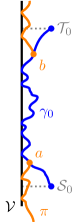
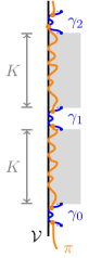
Figure 1. Left: The polymer $\gamma_{0}$ (blue) is a local highway. The polymer $\pi$ (orange) hits $\gamma_{0}$ for the first time at $a$ and for the last time at $b$. Its trajectory between $a$ and $b$ has been replaced by that of $\gamma_{0}$. In accordance with our assumption $j=o(J)$, we have depicted $\mathcal{S}_{0},\mathcal{T}_{0}$ as being much shorter than the vertical distance between the two segments. Right: Three local highways $\gamma_{0},\gamma_{1},\gamma_{2}$ (blue) are separated by a vertical distance of $K$ (the scale is much larger than in the left figure). Their respective laws (polymer measures) are each determined by the weights inside of a $J\times J$ box. As $J=o(K)$, these boxes are disjoint and therefore the laws are $\mathbb{P}$-independent. As $\pi$ (orange) coalesces with each $\gamma_{i}$, it follows similarly that the laws of the segments of $\pi$ within the shaded gray strips are $\mathbb{P}$-independent.

In Section 5 we make this precise, and extend it to hold simultaneously for $(n/K)$-many pairs $\mathcal{S}_{i},\mathcal{T}_{i}$ and local highways $\gamma_{i}$. The behavior of $\pi$ inside the $i$-th box (of area $J^{2}\asymp\mathrm{polylog}(n)$) has a negligible effect on the diffusively-scaled free energy. This leads to an approximation of the form

$$\frac{F(0,0,0,n)-\mathbb{E}\left[F(0,0,0,n)\right]}{\sqrt{n}}\approx\frac{1}{\sqrt{n/K}}\sum_{i=1}^{n/K}\frac{F_{i}-\mathbb{E}\left[F_{i}\right]}{\sqrt{K}},$$

where the $F_{i}$ are independent random variables, each being (approximately) the contribution made to $F(0,0,0,n)$ by the polymer $\pi$ during its journey from $\mathcal{T}_{i}$ to $\mathcal{S}_{i+1}$.

Finally, since $n/K\to\infty$, we have reduced the problem to that of verifying the hypotheses of the classical Lindeberg central limit theorem for a diffusively-scaled sum of $(n/K)$-many independent random variables $X_{i}\coloneqq\frac{F_{i}-\mathbb{E}\left[F_{i}\right]}{\sqrt{K}}$ with variance $\operatorname{Var}(X_{i})\asymp 1$ (the aforementioned variance estimates imply $\operatorname{Var}(F_{i})\asymp K$). We show that the $X_{i}$ satisfy the Lindeberg condition in Section 7 via a straightforward martingale concentration argument that does not depend on polymer pinning.

Remark 1.12 (Alternative proof of Gaussian fluctuations at zero temperature).

It turns out that geodesic pinning can be used to provide a much cleaner proof of Theorem 1.6 for the LPP model $G=L$ than what we outlined above. We sketch this now.

Assuming LLN separation, Theorem 1.4 implies that the left-most geodesic $\Gamma:(0,-m)\to(0,n)$ typically hits $\mathcal{V}$ at $\Theta(n+m)$-many locations. For $i\in\mathbb{Z}$, let $H_{i}$ be the energy that $\Gamma$ accrues during its journey between the pair of consecutive hitting locations straddling the horizontal line $\mathbb{Z}\times\{i\}$. Using that $|\Gamma\cap\mathcal{V}|=\Theta(n+m)$, one can adapt (and substantially simplify) the coalescence arguments of Section 5 to prove that the correlation between $H_{i}$ and $H_{j}$ decays as a stretched exponential in $|i-j|$. A further application of coalescence allows to take the limit $n,m\to\infty$, yielding a sequence $(\mathfrak{H}_{i})_{i\in\mathbb{Z}}$. One can show that $(\mathfrak{H}_{i})_{i\in\mathbb{Z}}$ inherits a stretched exponential rate of mixing from the prelimit, and that $(\mathfrak{H}_{i})_{i\in\mathbb{Z}}$ is stationary as a result of the vertical translation-invariance of the environment. One can further show that, under diffusive scaling, the last passage time $L(0,-m,0,n)$ is approximated by a sum of the $\mathfrak{H}_{i}$. The asymptotic Gaussianity then follows from classical results on the central limit theorem for stationary mixing sequences (e.g. [IL71, Bol82]). That $\operatorname{Var}(L(0,-m,0,n))=\Theta(n+m)$ can be proved as in Section 4, but with some simplifications owing to the stretched exponential mixing.

A remark to this effect previously appeared in [BSS16], where the authors resolved the famous slow bond problem by establishing LLN separation for a full-space LPP model with reinforced weights on a line. They further observed that LLN separation implies the pinning of the geodesic to the line, and explained how this can be used to construct the process $(\mathfrak{H}_{i})_{i\in\mathbb{Z}}$ and deduce the Gaussian fluctuations of the last passage time. Subsequently, Basu–Sarkar–Sly [BSS17] used geometric arguments to resolve several outstanding conjectures of Liggett related to the slow bond problem. In the course of their analysis they proved the pinning of the geodesic, and as a corollary provided the details of the argument of [BSS16] for the Gaussian fluctuations (see [BSS17, Appendix B]).

Unlike the last passage time, the positive temperature free energy depends on every path and consequently cannot be analyzed using only the elegant theory of stationary sequences. We therefore take a mesoscopic approach that allows to treat the zero and positive temperature models in a unified manner.

1.4. Organization of the paper

In Section 2.1 we record some notation. The remainder of Section 2 is spent collecting general results on the directed polymer model: a large deviations estimate in Section 2.2, LLN comparisons in Section 2.3, the phenomena of polymer ordering and coalescence in Section 2.4, and the correspondence between the positive temperature and zero temperature model in Section 2.5. In Section 3 we prove Theorem 1.4. In Section 4 we prove that the free energy $(0,0)\to(0,n)$ has variance $\Theta(n)$. In Section 5 we construct independent random variables whose sum approximates the diffusively-scaled free energy. In Section 6 we prove Corollary 1.10. In Section 7 we verify the Lindeberg condition for the random variables constructed in Section 5, thereby completing the proof of Theorem 1.6.

1.5. Acknowledgements

I am grateful to my advisor Shirshendu Ganguly for suggesting this problem and for numerous helpful discussions, insights, and comments on drafts of this paper. This work was supported by the National Science Foundation Graduate Research Fellowship Program under Grant No. DGE-2146752.

2. Preliminaries

2.1. Notation

We denote by $C,C^{\prime},C^{\prime\prime},C^{\prime\prime\prime}$ deterministic, strictly positive constants whose values may change from line to line (or in the same line), and which may depend on the law of the environment $\omega$, but not on any other parameters (such as $n$).

We follow the standard Landau asymptotic notation: we write $A=O(B)$ if $|A|\leq CB$ for some $C>0$, and $A=\Theta(B)$ if $A=O(B)$ and $B=O(A)$. We will frequently write $A\lesssim B$ instead of $A=O(B)$, $A\gtrsim B$ instead of $B=O(A)$, and $A\asymp B$ instead of $A=\Theta(B)$. Lastly, we write $A=o(1)$ if $\lim_{n\to\infty}A=0$, and $A=o(B)$ if $\frac{A}{B}=o(1)$.

2.2. Large deviations

In this section we prove a large deviations estimate for the free energy. For $G\in\{F,L\}$ we define

$$\Upsilon=\Upsilon(G)\coloneqq\frac{g-g^{\mathrm{bulk}}}{5},$$ (2.1)

so that LLN separation (1.2) is equivalent to $\Upsilon>0$.

Lemma 2.1 (Free energy large deviations).

There exist constants $C,C^{\prime},c_{0}>0$ depending only on the law of $\omega$ such that the following holds. Fix $G\in\{F,L\}$ and suppose the polymer model has LLN separation. Then for all $u=(x_{1},t_{1}),v=(x_{2},t_{2})\in\mathcal{H}$ with vertical displacement $t_{2}-t_{1}\geq c_{0}$ and $\Pi(u,v)\neq\varnothing$, we have that

$$\mathbb{P}\left(\bigl{|}G(u,v)-\mathbb{E}\left[G(u,v)\right]\bigr{|}>\Upsilon|t_{2}-t_{1}|\right)\leq C\exp\left(-C^{\prime}\min\{1,\Upsilon^{2}\}\,|t_{2}-t_{1}|^{1/3}\right)$$ (2.2)

and that

$$\mathbb{P}\left(\bigl{|}G^{\mathrm{bulk}}(u,v)-\mathbb{E}\bigl{[}G^{\mathrm{bulk}}(u,v)\bigr{]}\bigr{|}>\Upsilon|t_{2}-t_{1}|\right)\leq C\exp\left(-C^{\prime}\min\{1,\Upsilon^{2}\}\,|t_{2}-t_{1}|^{1/3}\right).$$ (2.3)

We will use the following fact in the proof of Lemma 2.1.

Lemma 2.2.

Fix $d\geq 1$ and define functions $h_{1},h_{2}:\mathbb{R}^{d}\to\mathbb{R}$ by

$$h_{1}(x)\coloneqq\log\left(\sum_{i=1}^{d}e^{x_{i}}\right),\quad\quad h_{2}(x)\coloneqq\max_{i\in\llbracket 1,\,d\rrbracket}x_{i}.$$

Then for $k\in\{1,2\}$, the function $h_{k}$ satisfies

$$|h_{k}(x)-h_{k}(y)|\leq\max_{i\in\llbracket 1,\,d\rrbracket}|x_{i}-y_{i}|,\quad\forall x,y\in[0,\infty)^{d}.$$

Proof of Lemma 2.2.

A direct calculation shows that the gradient $\nabla h_{1}$ has $\ell^{1}$-norm $\left\lVert\nabla h_{1}(x)\right\rVert_{1}=1$ for all $x\in\mathbb{R}^{d}$. The inequality follows from the mean value theorem. As for $h_{2}$, Lemma 2.2 is just the reverse triangle inequality for the $\ell^{\infty}$-norm, restricted to the nonnegative orthant $[0,\infty)^{d}$. ∎

Proof of Lemma 2.1.

For notational simplicity we only prove (2.2), but the same argument works for (2.3). By translation-invariance in the vertical direction, it suffices to treat the case $u=(x_{1},0),v=(x_{2},t)$. Consider the truncated environment $\widehat{\omega}$ given by

$$\widehat{\omega}(y,s)\coloneqq\omega(y,s)\wedge t^{1/3}\quad\text{for }(y,s)\in\mathcal{H}.$$

Let $\widehat{G}$ be the free energy $u\to v$ in $\widehat{\omega}$. For $j\in\mathbb{Z}$ we denote by $\mathscr{F}_{j}$ the $\sigma$-algebra generated by $\widehat{\omega}$ up to height $j$, that is, $\mathscr{F}_{j}\coloneqq\sigma\bigl{(}\widehat{\omega}(y,s):y\in\mathbb{Z}_{\geq 0},\;s\leq j\bigr{)}$. We first show that

$$\left|\mathbb{E}\left[\widehat{G}\>|\>\mathscr{F}_{j}\right]-\mathbb{E}\left[\widehat{G}\>|\>\mathscr{F}_{j-1}\right]\right|\leq 2t^{1/3}\quad\text{for all }j\in\llbracket 0,t\rrbracket.$$ (2.4)

For this we mimic an argument of [Kes93]. Fix a realization of the environment $\widehat{\omega}$. Also fix $j\in\llbracket 0,t\rrbracket$ and let $\widehat{\omega}^{\prime}$ be the environment obtained from $\widehat{\omega}$ by replacing $\widehat{\omega}(y,j)$ with an independent copy $\widehat{\omega}^{\prime}(y,j)$ for each $y\in\mathbb{Z}_{\geq 0}$. For any path $\pi:u\to v$, we have

$$\left|\sum_{(y,s)\in\pi}\widehat{\omega}(y,s)-\sum_{(y,s)\in\pi}\widehat{\omega}^{\prime}(y,s)\right|=\bigl{|}\widehat{\omega}(\pi(j),j)-\widehat{\omega}^{\prime}(\pi(j),j)\bigr{|}\leq 2t^{1/3}.$$ (2.5)

By Lemma 2.2,

$$\left|\widehat{G}-\widehat{G}^{\prime}\right|\leq\sup_{\pi\in\Pi(u,v)}\left|\sum_{(y,s)\in\pi}\widehat{\omega}(y,s)-\sum_{(y,s)\in\pi}\widehat{\omega}^{\prime}(y,s)\right|,$$

where $\widehat{G}^{\prime}$ denotes the free energy $u\to v$ in $\widehat{\omega}^{\prime}$. We substitute the above inequality into (2.5) and average over $(\widehat{\omega}^{\prime}(y,s))_{s\geq j,\,y\in\mathbb{Z}_{\geq 0}}$ to conclude (2.4).

Having shown (2.4), we may apply the Azuma–Hoeffding inequality to $\widehat{G}$. This yields constants $C,C^{\prime}>0$ depending only on the law of $\widehat{\omega}$ such that for all $z>0$,

$$\mathbb{P}\left(\bigl{|}\widehat{G}-\mathbb{E}[\widehat{G}]\bigr{|}>zt\right)\leq C\exp\left(-C^{\prime}\frac{z^{2}t^{2}}{\sum_{i=0}^{t}t^{2/3}}\right)\leq C\exp\left(-C^{\prime}z^{2}t^{1/3}\right).$$ (2.6)

We now estimate the error introduced by truncating the weights. We begin by observing that $\widehat{G}$ and $G\coloneqq G(x_{1},0,x_{2},t)$ depend only on the weights inside the box

$$\mathcal{B}\coloneqq\llbracket\min\{x_{1},x_{2}\}-t,\;\max\{x_{1},x_{2}\}+t\rrbracket\times\llbracket 0,t\rrbracket.$$

As $\Pi(x_{1},0,x_{2},t)\neq\varnothing$, it follows that the box $\mathcal{B}$ has area $|\mathcal{B}|\leq Ct^{2}$ for some absolute constant $C>0$ that does not depend on $x_{1},x_{2},t$. Therefore, a union bound over $\mathcal{B}$ yields

$$\begin{split}\mathbb{P}\bigl{(}G\neq\widehat{G}\bigr{)}&\leq\mathbb{P}\left(\sup_{(y,s)\in\mathcal{B}}\omega(y,s)>t^{1/3}\right)\\ &\leq Ct^{2}\exp(-C^{\prime}t^{1/3})\\ &\leq C\exp(-C^{\prime}t^{1/3}),\end{split}$$ (2.7)

where we used the fact that $\mathsf{X},\mathsf{Y}$ are subexponential. Combining (2.7) with the inequality

$$G-\widehat{G}\leq L(x_{1},0,x_{2},t)+\log|\Pi(x_{1},0,x_{2},t)|\leq\sum_{(y,s)\in\mathcal{B}}\omega(y,s)+t\log 4$$

and the Cauchy–Schwarz inequality, we get

$$\begin{split}0\leq\mathbb{E}\left[G-\widehat{G}\right]&=\mathbb{E}\left[\bigl{(}G-\widehat{G}\bigr{)}\mathbf{1}_{\{G\neq\widehat{G}\}}\right]\\ &\leq C\,\mathbb{E}\left[\left(\sum_{(y,s)\in\mathcal{B}}\omega(y,s)+t\log 4\right)^{2}\right]^{1/2}\exp(-C^{\prime}t^{1/6})\\ &\leq Ct^{2}\exp(-C^{\prime}t^{1/6})\\ &\leq C\exp(-C^{\prime}t^{1/6}),\end{split}$$ (2.8)

where $C,C^{\prime}$ depend only on the law of $\omega$. By our hypothesized LLN separation (i.e. $\Upsilon>0$), we can choose a constant $c_{0}>0$ depending only on $C,C^{\prime},\Upsilon$, such that

$$C\exp(-C^{\prime}t^{1/6})<\frac{\Upsilon}{2}t\quad\text{for all }t\geq c_{0}.$$ (2.9)

Then, combining (2.6), (2.7), and (2.8), we conclude that for $t\geq c_{0}$,

$$\begin{split}\mathbb{P}\bigl{(}|G-\mathbb{E}\left[G\right]|>\Upsilon t\bigr{)}&\leq\mathbb{P}\left(\bigl{|}\widehat{G}-\mathbb{E}[\widehat{G}]\bigr{|}+\bigl{|}\mathbb{E}\left[G\right]-\mathbb{E}[\widehat{G}]\bigr{|}>\Upsilon t\right)+\mathbb{P}\left(G\neq\widehat{G}\right)\\ &\leq\mathbb{P}\left(\bigl{|}\widehat{G}-\mathbb{E}[\widehat{G}]\bigr{|}>\frac{\Upsilon}{2}t\right)+C\exp\left(-C^{\prime}t^{1/3}\right)\\ &\leq C\exp\left(-C^{\prime}\Upsilon^{2}t^{1/3}\right)+C\exp\left(-C^{\prime}t^{1/3}\right).\end{split}$$ (2.10)

This proves Lemma 2.1. ∎

Remark 2.3 (Suboptimality of Lemma 2.1).

Lemma 2.1 is far from sharp. For instance, the proof implies the same result with $\Upsilon$ replaced by any fixed $z>0$, provided that $c_{0}$ is increased (depending on $z$). Faster tail decay rates are also known (e.g. [LW09]). However, we are not aware of a suitable estimate in the literature that applies simultaneously to the zero temperature and positive temperature models. Lemma 2.1 suffices for our purposes as-is, so we did not attempt to optimize it further.

2.3. LLN comparisons

We now record two LLN comparisons with the aim of streamlining our upcoming applications of LLN separation. We introduce full-space analogues of the objects from Definition 1.1. Let $\Pi_{\mathrm{full}}(x_{1},t_{1},x_{2},t_{2})$ be the set of all lattice paths with steps in $\{(-1,1),(1,1)\}$ joining $(x_{1},t_{1})$ to $(x_{2},t_{2})$, not only those confined to the half-space $\mathcal{H}$. We extend the environment $\omega^{\mathrm{bulk}}$ to a full-space environment of i.i.d. copies of $\mathsf{X}$ and define

$$F^{\mathrm{bulk}}_{\mathrm{full}}(x_{1},t_{1},x_{2},t_{2})\coloneqq\log\left(\sum_{\pi\in\Pi_{\mathrm{full}}(x_{1},t_{1},x_{2},t_{2})}\exp\left(\sum_{(x,t)\in\pi}\omega^{\mathrm{bulk}}(x,t)\right)\right)$$

and

$$L^{\mathrm{bulk}}_{\mathrm{full}}(x_{1},t_{1},x_{2},t_{2})\coloneqq\sup_{\pi\in\Pi_{\mathrm{full}}(x_{1},t_{1},x_{2},t_{2})}\sum_{(x,t)\in\pi}\omega^{\mathrm{bulk}}(x,t).$$

We fix $G\in\{F,L\}$ and write $g\coloneqq f$ or $g\coloneqq\ell$ accordingly. Consider the sets of directions

$$D\coloneqq\{\theta\in\mathbb{R}^{2}\setminus\{(0,0)\}:\theta_{2}\geq\theta_{1}\geq 0\},\quad\quad D_{\mathrm{full}}\coloneqq\{\theta\in\mathbb{R}^{2}\setminus\{(0,0)\}:\theta_{2}\geq|\theta_{1}|\}.$$

We extend (1.1) by setting

$$g^{\mathrm{bulk}}(\theta)\coloneqq\lim_{n\to\infty}\frac{\mathbb{E}\left[G^{\mathrm{bulk}}(0,0,2\lfloor n\theta_{1}/2\rfloor,2\lfloor n\theta_{2}/2\rfloor)\right]}{n},\quad\quad\theta\in D,$$

and

$$g^{\mathrm{bulk}}_{\mathrm{full}}(\theta)\coloneqq\lim_{n\to\infty}\frac{\mathbb{E}\left[G^{\mathrm{bulk}}_{\mathrm{full}}(0,0,2\lfloor n\theta_{1}/2\rfloor,2\lfloor n\theta_{2}/2\rfloor)\right]}{n},\quad\quad\theta\in D_{\mathrm{full}},$$

where $\lfloor\cdot\rfloor$ is the floor function. These limits exist by superadditivity. It follows that $g^{\mathrm{bulk}}(\lambda\theta)=\lambda g^{\mathrm{bulk}}(\theta)$ and $g^{\mathrm{bulk}}_{\mathrm{full}}(\lambda\theta)=\lambda g^{\mathrm{bulk}}(\theta)$ for any $\lambda>0$.

Write $\mathbf{e}_{2}\coloneqq(0,1)\in D$. The vertical bulk free energy $g^{\mathrm{bulk}}$ appearing in (1.1) is presently denoted by $g^{\mathrm{bulk}}(\mathbf{e}_{2})$. The following lemma asserts that in an i.i.d. environment, the half-space vertical LLN coincides with the full-space vertical LLN.

Lemma 2.4.

$g^{\mathrm{bulk}}_{\mathrm{full}}(\mathbf{e}_{2})=g^{\mathrm{bulk}}(\mathbf{e}_{2})$.

Proof.

The inequality $g^{\mathrm{bulk}}_{\mathrm{full}}(\mathbf{e}_{2})\geq g^{\mathrm{bulk}}(\mathbf{e}_{2})$ follows from the fact that $\Pi(0,0,0,n)\subset\Pi_{\mathrm{full}}(0,0,0,n)$. For the reverse inequality, we first fix $\varepsilon>0$ and choose an even integer $k=k(\varepsilon)>0$ such that

$$\frac{\mathbb{E}\left[G^{\mathrm{bulk}}_{\mathrm{full}}(0,0,0,k)\right]}{k}\geq g^{\mathrm{bulk}}_{\mathrm{full}}(\mathbf{e}_{2})-\varepsilon.$$ (2.11)

Using superadditivity and the fact that the free energies are $\geq 0$ almost surely, we get

$$G^{\mathrm{bulk}}(0,0,0,n)\geq\sum_{i=2}^{n/k-3}G^{\mathrm{bulk}}\left(\frac{k+4}{2},\;ik,\;\frac{k+4}{2},\;(i+1)k\right).$$ (2.12)

On the other hand, any full-space path $\pi\in\Pi_{\mathrm{full}}(0,0,0,n)$ satisfying

$$\pi(ik)=\frac{k+4}{2}\quad\text{for all }i\in\llbracket 2,\,n/k-2\rrbracket$$ (2.13)

must also satisfy $\pi\cap\mathcal{H}_{\llbracket 2k,\,n-2k\rrbracket}\subset\mathcal{H}\setminus\mathcal{V}$ (cf. Remark 1.5). Therefore for $i\in\llbracket 2,\,n/k-3\rrbracket$,

$$G^{\mathrm{bulk}}\left(\frac{k+4}{2},\;ik,\;\frac{k+4}{2},\;(i+1)k\right)=G^{\mathrm{bulk}}_{\mathrm{full}}\left(\frac{k+4}{2},\;ik,\;\frac{k+4}{2},\;(i+1)k\right).$$ (2.14)

By (2.11), (2.12), (2.13), (2.14), and vertical translation-invariance,

$$\begin{split}\frac{\mathbb{E}\left[G^{\mathrm{bulk}}(0,0,0,n)\right]}{n}&\geq\frac{1}{n}\sum_{i=2}^{n/k-3}\mathbb{E}\left[G^{\mathrm{bulk}}_{\mathrm{full}}\left(\frac{k+4}{2},\;ik,\;\frac{k+4}{2},\;(i+1)k\right)\right]\\ &=\left(\frac{1}{k}-\frac{4}{n}\right)\mathbb{E}\left[G^{\mathrm{bulk}}_{\mathrm{full}}\left(0,0,0,k\right)\right]\\ &\geq g^{\mathrm{bulk}}_{\mathrm{full}}(\mathbf{e}_{2})-\varepsilon-O(1/n).\end{split}$$

Let $n\to\infty$ to get $g^{\mathrm{bulk}}(\mathbf{e}_{2})\geq g^{\mathrm{bulk}}_{\mathrm{full}}(\mathbf{e}_{2})-\varepsilon$, then let $\varepsilon\downarrow 0$. ∎

The next lemma will help us establish pinning for polymers whose endpoints do not lie on $\mathcal{V}$.

Lemma 2.5 (Vertical LLN dominates).

For all $\theta\in D_{\mathrm{full}}$ with $\ell^{1}$-norm $\left\lVert\theta\right\rVert_{1}=1$,

$$g^{\mathrm{bulk}}(\mathbf{e}_{2})\geq g^{\mathrm{bulk}}_{\mathrm{full}}(\theta).$$

In particular, LLN separation (1.2) implies that $g>g^{\mathrm{bulk}}_{\mathrm{full}}(\theta)$ for all $\theta\in D_{\mathrm{full}}$ with $\left\lVert\theta\right\rVert_{1}=1$.

Proof.

Write $\mathbf{0}\coloneqq(0,0)$. By superadditivity,

$$\mathbb{E}\left[G^{\mathrm{bulk}}_{\mathrm{full}}(\mathbf{0},n\mathbf{e}_{2})\right]\geq\mathbb{E}\left[G^{\mathrm{bulk}}_{\mathrm{full}}(\mathbf{0},2\lfloor n\theta/4\rfloor)\right]+\mathbb{E}\left[G^{\mathrm{bulk}}_{\mathrm{full}}(2\lfloor n\theta/4\rfloor,n\mathbf{e}_{2})\right]-O(1),$$

where the $O(1)$ error is from double-counting $\omega^{\mathrm{bulk}}(2\lfloor n\theta/4\rfloor)$. Here we apply $\lfloor\cdot\rfloor$ entry-wise. On the other hand, by symmetry we have

$$\mathbb{E}\left[G^{\mathrm{bulk}}_{\mathrm{full}}(\mathbf{0},2\lfloor n\theta/4\rfloor)\right]=\mathbb{E}\left[G^{\mathrm{bulk}}_{\mathrm{full}}(2\lfloor n\theta/4\rfloor,n\mathbf{e}_{2})\right]+O(1),$$

where the $O(1)$ error is from taking $\lfloor\cdot\rfloor$. Therefore

$$g^{\mathrm{bulk}}_{\mathrm{full}}(\mathbf{e}_{2})=g^{\mathrm{bulk}}(\mathbf{e}_{2})\geq 2g^{\mathrm{bulk}}_{\mathrm{full}}(\theta/2)=g^{\mathrm{bulk}}_{\mathrm{full}}(\theta),$$

where the first equality is by Lemma 2.4. ∎

In the sequel we resume our use of the abbreviation $g^{\mathrm{bulk}}\coloneqq g^{\mathrm{bulk}}(\mathbf{e}_{2})$.

2.4. Polymer ordering and coalescence

Recall the polymer ordering phenomenon described in Section 1.1: the path which is pointwise the left-most of two geodesics is itself a geodesic. In particular, for any $u,v\in\mathcal{H}$ with $\Pi(u,v)\neq\varnothing$, there exists a unique left-most geodesic $u\to v$. This uniqueness implies that when two left-most geodesics intersect, they coalesce, sharing as much of their remaining journeys as possible:

Lemma 2.6 (Geodesic coalescence).

Fix $u,u^{\prime},v,v^{\prime}\in\mathcal{H}$ and let $\Gamma_{u,v}:u\to v,\,\Gamma_{u^{\prime},v^{\prime}}:u^{\prime}\to v^{\prime}$ be left-most geodesics. The following holds almost surely. If $\Gamma_{u,v}(r)=\Gamma_{u^{\prime},v^{\prime}}(r)$ for some $r$, and $\Gamma_{u,v}(s)\neq\Gamma_{u^{\prime},v^{\prime}}(s)$ for some $s>r$, then $\Gamma_{u,v}(t)\neq\Gamma_{u^{\prime},v^{\prime}}(t)$ for all $t\geq s$. In other words, the intersection $\Gamma_{u,v}\cap\Gamma_{u^{\prime},v^{\prime}}$ is a connected subset of $\mathcal{H}$.

Proof.

Suppose there exists $r$ such that $\Gamma_{u,v}(r)=\Gamma_{u^{\prime},v^{\prime}}(r)$ and $\Gamma_{u,v}(r+1)\neq\Gamma_{u^{\prime},v^{\prime}}(r+1)$. Assume for the sake of contradiction that $\Gamma_{u,v},\Gamma_{u^{\prime},v^{\prime}}$ intersect above height $r+1$. Let $t$ be the first height at which such an intersection occurs, i.e. $t\coloneqq\min\{s>r+1:\Gamma_{u,v}(s)=\Gamma_{u^{\prime},v^{\prime}}(s)\}.$ Then restricting $\Gamma_{u,v},\Gamma_{u^{\prime},v^{\prime}}$ to the strip $\mathcal{H}_{\llbracket r,t\rrbracket}$ produces two geodesics $(\Gamma_{u,v}(r),r)\to(\Gamma_{u,v}(t),t)$, one of which lies strictly to the left of the other (except at the starting and ending points). This contradicts uniqueness. ∎

The following lemma establishes positive temperature analogues of the above notions.

Lemma 2.7 (Positive temperature polymer ordering and coalescence).

Fix points $u=(x_{1},t_{1}),u^{\prime}=(y_{1},t_{1}),v=(x_{2},t_{2}),v^{\prime}=(y_{2},t_{2})\in\mathcal{H}$ with $t_{1}<t_{2}$ and $x_{i}\leq y_{i}$ for $i=1,2$. Let $\pi_{u,v}:u\to v$ and $\pi_{u^{\prime},v^{\prime}}:u^{\prime}\to v^{\prime}$ be polymers, i.e. paths distributed according to $\mathbb{Q}^{u,v}$ and $\mathbb{Q}^{u^{\prime},v^{\prime}}$, respectively. There exists a coupling of $\mathbb{Q}^{u,v},\mathbb{Q}^{u^{\prime},v^{\prime}}$ under which the following hold:

1. $\pi_{u,v}$ lies to the left of $\pi_{u^{\prime},v^{\prime}}$, and

2. $\pi_{u,v}\cap\pi_{u^{\prime},v^{\prime}}$ is a connected subset of $\mathcal{H}$.

Proof.

We fix a realization of the environment $\omega$, so that the only randomness in the following discussion is from the underlying random walk.

We first construct a coupling with the desired properties in the case $v=v^{\prime}$. Fix independent polymers

$$\pi_{u,v}:u\to v,\quad\quad\pi_{u^{\prime},v}:u^{\prime}\to v.$$

We view $\pi_{u,v},\pi_{u^{\prime},v}$ as functions $\llbracket t_{1},t_{2}\rrbracket\to\mathbb{Z}_{\geq 0}$ and define a $\mathbb{Z}_{\geq 0}\times\mathbb{Z}_{\geq 0}$-valued process $\bm{\pi}$ by

$$\bm{\pi}(t)\coloneqq(\pi_{u,v}(t),\pi_{u^{\prime},v}(t)).$$

Let $\mathscr{G}=(\mathscr{G}_{t})_{t\in\llbracket t_{1},t_{2}\rrbracket}$ be the natural filtration induced by $\bm{\pi}$, and consider the $\mathscr{G}$-stopping time

$$\tau\coloneqq\inf\{t:\pi_{u,v}(t)=\pi_{u^{\prime},v}(t)\}.$$

Write $T=(\pi_{u,v}(\tau),\tau)$. Let $\pi_{u,v}^{-}$ be the segment of $\pi_{u,v}$ from $u$ to $T$, and let $\pi_{u,v}^{+}$ be the segment of $\pi_{u,v}$ from $T$ to $v$. Define $\pi_{u^{\prime},v}^{\pm}$ analogously. It follows from the independence of $\pi_{u,v},\pi_{u^{\prime},v}$ that $\bm{\pi}$ satisfies the strong Markov property. Therefore the pairs $(\pi_{u,v}^{-},\pi_{u^{\prime},v}^{-})$ and $(\pi_{u,v}^{+},\pi_{u^{\prime},v}^{+})$ are conditionally independent given $T$. Moreover, $\pi_{u,v}^{+}$ and $\pi^{+}_{u^{\prime},v}$ are conditionally independent given $\mathscr{G}_{\tau}$, with the same conditional law (the polymer measure $\mathbb{Q}^{T,v}$). Let $\widetilde{\pi}_{u,v}$ be the path $u\to v$ obtained from $\pi_{u,v}$ by replacing $\pi_{u,v}^{+}$ with $\pi_{u^{\prime},v}^{+}$. By construction $\widetilde{\pi}_{u,v}$ lies to the left of $\pi_{u^{\prime},v}$, and the preceding discussion ensures that the joint law of $(\widetilde{\pi}_{u,v},\pi_{u^{\prime},v})$ has marginals $\mathbb{Q}^{u,v},\mathbb{Q}^{u^{\prime},v}$. This is illustrated on the left side of Figure 2 on page 2.

Assume now $v\neq v^{\prime}$. Fix a sample $(\widetilde{\pi}_{u,v},\pi_{u^{\prime},v})$ from the coupling constructed above, as well as an independent sample $\pi_{u^{\prime},v^{\prime}}$. By reversibility of the random walk, we can view $\pi_{u^{\prime},v^{\prime}}$ as a sample from $\mathbb{Q}^{v^{\prime},u^{\prime}}$, the polymer measure defined in terms of paths $v^{\prime}\to u^{\prime}$ with steps in $\{(1,-1),(-1,-1)\}$. We can similarly view $\pi_{u^{\prime},v}$ as a sample from $\mathbb{Q}^{v^{\prime},u}$. The argument of the previous paragraph yields a path $\widetilde{\pi}_{u^{\prime},v^{\prime}}$ such that

• $\widetilde{\pi}_{u^{\prime},v^{\prime}}$ lies to the right of $\pi_{u^{\prime},v}$,

• $\widetilde{\pi}_{u^{\prime},v^{\prime}}\cap\pi_{u^{\prime},v}$ is connected, and

• the joint law of $(\widetilde{\pi}_{u^{\prime},v^{\prime}},\pi_{u^{\prime},v})$ has marginals $\mathbb{Q}^{u^{\prime},v^{\prime}},\mathbb{Q}^{u^{\prime},v}$.

By averaging over $\pi_{u^{\prime},v}$, we conclude that $(\widetilde{\pi}_{u,v},\widetilde{\pi}_{u^{\prime},v^{\prime}})$ is a coupling of $\mathbb{Q}^{u,v},\mathbb{Q}^{u^{\prime},v^{\prime}}$ under which properties (a) and (b) above hold (see Figure 2 on page 2). ∎

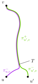
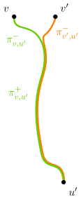
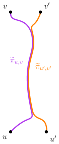
Figure 2. Left: The polymers $\pi_{u,v}$ (purple) and $\pi_{u^{\prime},v}$ (green) begin their respective journeys at $u$ and $u^{\prime}$. Their first intersection point is labeled $T$. The trajectory of $\pi_{u,v}$ after $T$ has been replaced by the trajectory of $\pi_{u^{\prime},v}$ after $T$.   Middle: The green path $\pi_{u^{\prime},v}$ appearing in the left figure is identified with a sample $\pi_{v,u^{\prime}}$ (also green) from the time-reversed polymer measure. The polymer $\pi_{v^{\prime},u^{\prime}}$ (orange) begins its journey at $v^{\prime}$ and at some (unlabeled) point hits $\pi_{v,u^{\prime}}$. The remaining trajectory of $\pi_{v^{\prime},u^{\prime}}$ has been replaced by that of $\pi_{v,u^{\prime}}$. ⁴  Right: We superimpose the left and middle figures, omitting the green path $\pi_{u^{\prime},v}=\pi_{v,u^{\prime}}$. The desired coupling is obtained by identifying the orange path with its time-reversal $u^{\prime}\to v^{\prime}$ and averaging over the (now hidden) green path. ⁴

2.5. Correspondence between positive temperature and zero temperature

Much of our analysis will apply simultaneously to the polymer free energy and the last passage time. Let us make explicit the relationship between the two.

For $\beta>0$ (to be thought of as inverse temperature), consider the partition function $Z_{\beta}\coloneqq\sum_{\pi}e^{\beta H(\pi)}$, the free energy $F_{\beta}\coloneqq\beta^{-1}\log Z_{\beta}$, and the polymer measure $\mathbb{Q}_{\beta}(\{\pi\})\coloneqq Z_{\beta}^{-1}e^{\beta H(\pi)}$. In the zero temperature limit $\beta\to\infty$, we have $F_{\beta}\to L$ and (formally) $\mathbb{Q}_{\beta}\to\delta_{\{\Gamma\}}$, the Dirac mass on the left-most geodesic $\Gamma$.

We have omitted $\beta$ from our definitions in Section 1.1, as it can be absorbed into the weights $\mathsf{X},\mathsf{Y}$. Accordingly, we replace the formal zero temperature limit with the following “tropicalization” correspondence: for any set of paths $A$ and any $c\in[0,1)$, we write

$$\begin{split}\mathbb{Q}\quad&\longmapsto\quad\delta_{\{\Gamma\}},\\ \{\omega:\mathbb{Q}(A)>c\}\quad&\longmapsto\quad\{\omega:\text{ the left-most geodesic }\Gamma\in A\},\\ \log\left(\sum_{\pi\in A}e^{H(\pi)}\right)\quad&\longmapsto\quad\sup_{\pi\in A}H(\pi),\\ Z\quad&\longmapsto\quad e^{L}.\end{split}$$ (2.15)

We will use this dictionary to streamline our presentation in the following manner. All the results below apply to the zero and positive temperature models simultaneously, and in our proofs we always treat the positive temperature model first. In many cases we will be able to convert the proof of the positive temperature statement into a proof of the zero temperature statement by formally replacing all instances of the symbols on the left side of (2.15) that appear in the positive temperature proof with the corresponding symbols on the right side of (2.15).

3. Pinning

In this section we prove Theorem 1.4, thereby establishing that LLN separation implies the pinning of the polymer to $\mathcal{V}$.

Fix $t_{1}<t_{2}$ and $x_{1},x_{2}\geq 0$. We denote by $\Pi^{\mathrm{exc}}(x_{1},t_{1},x_{2},t_{2})$ the set of excursions $(x_{1},t_{1})\to(x_{2},t_{2})$, i.e. paths that do not hit $\mathcal{V}$ (unless $x_{1}=0$ or $x_{2}=0$):

$$\Pi^{\mathrm{exc}}(x_{1},t_{1},x_{2},t_{2})\coloneqq\left\{\pi\in\Pi(x_{1},t_{1},x_{2},t_{2}):\pi\cap\mathcal{V}\subset\{(0,t_{1}),(0,t_{2})\}\right\}.$$

The following lemma asserts that, under LLN separation, excursions typically are not competitive with paths that hit $\mathcal{V}$.

Lemma 3.1 (Excursions are rare).

There exist constants $C,C^{\prime},k_{0}>0$ depending only on the law of $\omega$ such that the following holds. Fix $G\in\{F,L\}$. Suppose the polymer model has LLN separation, i.e. $\Upsilon>0$. Fix $(x_{1},t_{1}),(x_{2},t_{2})$ satisfying $t_{2}-t_{1}\geq k_{0}(x_{1}+x_{2}+1)$ and $\Pi(x_{1},t_{1},x_{2},t_{2})\neq\varnothing$. If $G=F$ then

$$\mathbb{P}\left(\mathbb{Q}^{(x_{1},t_{1}),(x_{2},t_{2})}\left(\Pi^{\mathrm{exc}}(x_{1},t_{1},x_{2},t_{2})\right)>e^{-\Upsilon(|t_{2}-t_{1}|+|x_{2}-x_{1}|)}\right)\leq C\exp\left(-C^{\prime}|t_{2}-t_{1}|^{1/3}\right).$$ (3.1)

If $G=L$ and we denote by $\Gamma$ the leftmost geodesic $(x_{1},t_{1})\to(x_{2},t_{2})$, then

$$\mathbb{P}\left(\Gamma\in\Pi^{\mathrm{exc}}(x_{1},t_{1},x_{2},t_{2})\right)\leq C\exp\left(-C^{\prime}|t_{2}-t_{1}|^{1/3}\right).$$ (3.2)

Proof.

We will prove (3.1). The correspondence of Section 2.5 will immediately yield (3.2).

Let us first record two properties of the bulk LLN $f^{\mathrm{bulk}}$. By superadditivity, (1.1), and Lemma 2.5, we have

$$\mathbb{E}\left[F^{\mathrm{bulk}}(x_{1},t_{1},x_{2},t_{2})\right]\leq f^{\mathrm{bulk}}\cdot(|t_{2}-t_{1}|+|x_{2}-x_{1}|).$$ (3.3)

By LLN separation (1.2), (2.1), there exists $k_{0}^{\prime}>0$ such that

$$\mathbb{E}\left[F(0,0,0,t)\right]\geq(f^{\mathrm{bulk}}+4\Upsilon)\,t\quad\text{for all even }t\geq k_{0}^{\prime}.$$ (3.4)

We now set $k_{0}\coloneqq k_{0}^{\prime}+c_{0}+2$, where $c_{0}$ is from Lemma 2.1. By vertical translation-invariance, it suffices to prove (3.1) for $\mathbb{Q}^{(x_{1},0),(x_{2},t)}$ with $t,x_{1},x_{2}\geq 0$ satisfying $t\geq k_{0}(x_{1}+x_{2}+1)$.

For simplicity we first treat the case $x_{1}=x_{2}=0$. We suppress the superscripts from the polymer measure and rewrite the left side of (3.1) as

$$\begin{split}\mathbb{P}\left(\mathbb{Q}(\Pi^{\mathrm{exc}}(0,0,0,t))>e^{-\Upsilon t}\right)&=\mathbb{P}\left(\log\mathbb{Q}(\Pi^{\mathrm{exc}}(0,0,0,t))>-\Upsilon t\right)\\ &=\mathbb{P}\left(F^{\mathrm{exc}}(0,0,0,t)>F(0,0,0,t)-\Upsilon t\right),\end{split}$$ (3.5)

where we define $F^{\mathrm{exc}}(x_{1},0,x_{2},t)\coloneqq\log\left(\sum_{\pi\in\Pi^{\mathrm{exc}}(x_{1},0,x_{2},t)}e^{H(\pi)}\right)$. Since a path $\pi\in\Pi^{\mathrm{exc}}(0,0,0,t)$ only collects bulk weights $\omega^{\mathrm{bulk}}(x,s)$ (except at its endpoints $\pi(0),\pi(t)$), we have the estimate

$$F^{\mathrm{exc}}(0,0,0,t)\leq F^{\mathrm{bulk}}(1,1,1,t-1)+\omega(0,0)+\omega(0,t).$$

On the other hand, we have that $F(0,0,0,t)=F(1,1,1,t-1)+\omega(0,0)+\omega(0,t)$. Write $F\coloneqq F(1,1,1,t-1)$ and $F^{\mathrm{bulk}}\coloneqq F^{\mathrm{bulk}}(1,1,1,t-1)$. By substituting the above display into (3.5) and applying (3.3), (3.4), and Lemma 2.1 (note that $t-2\geq k_{0}-2\geq c_{0}$), we conclude that

$$\begin{split}\mathbb{P}\left(\mathbb{Q}(\Pi^{\mathrm{exc}}(0,0,0,t))>e^{-\Upsilon t}\right)&\leq\mathbb{P}\left(F<F^{\mathrm{bulk}}+\Upsilon t\right)\\ &\leq\mathbb{P}\left(F<(f^{\mathrm{bulk}}+\Upsilon)(t-2)+\Upsilon t\right)\\ &\quad\quad\quad+\mathbb{P}\left(F^{\mathrm{bulk}}>(f^{\mathrm{bulk}}+\Upsilon)(t-2)\right)\\ &\leq\mathbb{P}\bigl{(}F<\mathbb{E}\left[F\right]-2\Upsilon(t-2)+2\Upsilon\bigr{)}\,+C\exp\bigl{(}-C^{\prime}t^{1/3}\bigr{)}\\ &\leq\mathbb{P}\bigl{(}F<\mathbb{E}\left[F\right]-\Upsilon(t-2)\bigr{)}\,+C\exp\bigl{(}-C^{\prime}t^{1/3}\bigr{)}\\ &\leq C\exp\bigl{(}-C^{\prime}t^{1/3}\bigr{)}.\end{split}$$ (3.6)

Here we absorbed the factor $\min\{1,\Upsilon^{2}\}$ from Lemma 2.1 into the constant $C^{\prime}$.

Suppose now that $x_{1}>0$ and $x_{2}>0$. It follows that

$$F^{\mathrm{exc}}(x_{1},0,x_{2},t)\leq F^{\mathrm{bulk}}(x_{1},0,x_{2},t).$$

On the other hand, by superadditivity and the fact that the free energies are positive almost surely,

$$\begin{split}F(x_{1},0,x_{2},t)&\geq F(x_{1},0,1,x_{1}-1)+F(0,x_{1},0,t-x_{2})+F(1,t-x_{2}+1,x_{2},t)\\ &\geq F(0,x_{1},0,t-x_{2}).\end{split}$$

We also note that by applying (3.4) and increasing $k_{0}$ as needed, we can assume that

$$(f^{\mathrm{bulk}}+2\Upsilon)(t+|x_{2}-x_{1}|)\leq\mathbb{E}\left[F\right]-\Upsilon(t-x_{2}-x_{1})\quad\text{whenever}\quad t\geq k_{0}(x_{1}+x_{2}+1).$$

In combination with the above three displays, the condition $\mathbb{Q}(\Pi^{\mathrm{exc}}(x_{1},0,x_{2},t))>e^{-\Upsilon(t+|x_{2}-x_{1}|)}$ implies a comparison of $F^{\mathrm{bulk}}\coloneqq F^{\mathrm{bulk}}(x_{1},0,x_{2},t)$ and $F\coloneqq F(0,x_{1},0,t-x_{2})$, as in (3.5). We obtain, as in (3.6),

$$\begin{split}\mathbb{P}\left(\mathbb{Q}(\Pi^{\mathrm{exc}}(x_{1},0,x_{2},t))>e^{-\Upsilon(t+|x_{2}-x_{1}|)}\right)&\leq\mathbb{P}\left(F<F^{\mathrm{bulk}}+\Upsilon(t+|x_{2}-x_{1}|)\right)\\ &\leq\mathbb{P}\left(F<(f^{\mathrm{bulk}}+2\Upsilon)(t+|x_{2}-x_{1}|)\right)\\ &\quad\quad\quad\quad+\mathbb{P}\left(F^{\mathrm{bulk}}>(f^{\mathrm{bulk}}+\Upsilon)(t+|x_{2}-x_{1}|)\right)\\ &\leq\mathbb{P}\bigl{(}F<\mathbb{E}\left[F\right]-\Upsilon(t-x_{2}-x_{1})\bigr{)}+C\exp\bigl{(}-C^{\prime}t^{1/3}\bigr{)}\\ &\leq C\exp\bigl{(}-C^{\prime}(t-x_{2}-x_{1})^{1/3}\bigr{)}\\ &\leq C\exp\bigl{(}-C^{\prime}t^{1/3}\bigr{)}.\end{split}$$

The cases $x_{1}=0,x_{2}>0$ and $x_{1}>0,x_{2}=0$ follow from a straightforward combination of the previous two arguments. We omit the details. ∎

We now deduce Theorem 1.4 from Lemma 3.1.

Proof of Theorem 1.4.

We will treat the case $G=F$. The case $G=L$ will then follow from the correspondence of Section 2.5.

Fix $s_{1},s_{2}\in\llbracket x_{1},\,t-x_{2}\rrbracket$ with $s_{2}-s_{1}\geq k_{0}$. Notice that if a path $\pi:(x_{1},0)\to(x_{2},t)$ does not intersect $\mathcal{V}_{\llbracket s_{1},\,s_{2}\rrbracket}$, then there exist $a\in\llbracket 0,\,s_{1}-1\rrbracket$ and $b\in\llbracket s_{2}+1,\,t\rrbracket$ such that

$$\pi\cap\mathcal{H}_{\llbracket a,b\rrbracket}\in\Pi^{\mathrm{exc}}(\pi(a),a,\pi(b),b).$$

We denote by $a_{\pi}$ the minimal such $a$, and by $b_{\pi}$ the maximal such $b$. Observe that $\pi(a_{\pi})\in\{0,x_{1}\}$ and $\pi(b_{\pi})\in\{0,x_{2}\}$. Moreover, $\pi(a_{\pi})\neq 0$ only if $a_{\pi}=0$, and $\pi(b_{\pi})\neq 0$ only if $b_{\pi}=t$. The idea now is to perform a union bound over the possible pairs $(a_{\pi},b_{\pi})$ and apply Lemma 3.1 to control the tails. To this end we record the following estimates for the relevant polymer measures.

Suppose $0<a\leq b<t$. From the inequality

$$Z(x_{1},0,x_{2},t)\geq Z(x_{1},0,1,a-1)\,Z(0,a,0,b)\,Z(b+1,1,x_{2},t),$$

we deduce that

$$\mathbb{Q}^{(x_{1},0),(x_{2},t)}\left(\pi\cap\mathcal{H}_{\llbracket a,\,b\rrbracket}\in\Pi^{\mathrm{exc}}(0,a,0,b)\right)\leq\mathbb{Q}^{(0,a),(0,b)}\left(\Pi^{\mathrm{exc}}(0,a,0,b)\right).$$

A similar argument shows that

$$\mathbb{Q}^{(x_{1},0),(x_{2},t)}\left(\pi\cap\mathcal{H}_{\llbracket 0,\,b\rrbracket}\in\Pi^{\mathrm{exc}}(x_{1},0,0,b)\right)\leq\mathbb{Q}^{(x_{1},0),(0,b)}\left(\Pi^{\mathrm{exc}}(x_{1},0,0,b)\right),$$

and that

$$\mathbb{Q}^{(x_{1},0),(x_{2},t)}\left(\pi\cap\mathcal{H}_{\llbracket a,\,t\rrbracket}\in\Pi^{\mathrm{exc}}(0,a,x_{2},t)\right)\leq\mathbb{Q}^{(0,a),(x_{2},t)}\left(\Pi^{\mathrm{exc}}(0,a,x_{2},t)\right).$$

Now we perform the union bound. In particular, observe that by choosing $\delta=\delta(k_{0},\Upsilon)>0$ sufficiently small and $C^{\prime\prime}=C^{\prime\prime}(k_{0},\Upsilon)>0$ sufficiently large (each depending only on $k_{0},\Upsilon$), we can ensure that the following estimate holds for any $s_{1},s_{2}$ satisfying the above hypotheses:

$$\begin{split}\mathbb{P}\biggl{(}\mathbb{Q}^{(x_{1},0),(x_{2},t)}\bigl{(}\pi\cap\mathcal{V}_{\llbracket s_{1},\,s_{2}\rrbracket}&=\varnothing\bigr{)}>C^{\prime\prime}e^{-\delta\Upsilon|s_{2}-s_{1}|}\biggr{)}\\ &\leq\sum_{\begin{subarray}{c}a<s_{1},\\ b>s_{2}\end{subarray}}\mathbb{P}\left(\mathbb{Q}^{(0,a),(0,b)}(\Pi^{\mathrm{exc}}(0,a,0,b))>e^{-\Upsilon|b-a|}\right)\\ &\quad+\sum_{a<s_{1}}\mathbb{P}\left(\mathbb{Q}^{(0,a),(x_{2},t)}\left(\Pi^{\mathrm{exc}}(0,a,x_{2},t)\right)>e^{-\Upsilon(|t-a|+x_{2})}\right)\\ &\quad+\sum_{b>s_{2}}\mathbb{P}\left(\mathbb{Q}^{(x_{1},0),(0,b)}\left(\Pi^{\mathrm{exc}}(x_{1},0,0,b)\right)>e^{-\Upsilon(b+x_{1})}\right)\\ &\quad+\mathbb{P}\left(\mathbb{Q}^{(x_{1},0),(x_{2},t)}(\Pi^{\mathrm{exc}}(x_{1},0,x_{2},t))>e^{-\Upsilon(t+|x_{2}-x_{1}|)}\right).\end{split}$$

Applying Lemma 3.1 to the terms on the right side of the above display yields Theorem 1.4. ∎

We conclude this section by recording two consequences of Theorem 1.4 that will be useful later. First is the following lemma, which asserts that the polymer has $O(1)$ transversal fluctuations under LLN separation. It is essentially duplicated from Remark 1.5, and we omit the proof.

Lemma 3.2 (Polymer $O(1)$ transversal fluctuations).

There exist constants $C,C^{\prime},C^{\prime\prime},C^{\prime\prime\prime},k_{0}>0$ depending only on the law of $\omega$ such that the following hold. Fix $G\in\{F,L\}$ and suppose the polymer model has LLN separation. Fix $t,x_{1},x_{2}\geq 0$ satisfying $t\geq k_{0}(x_{1}+x_{2}+1)$ and $\Pi(x_{1},0,x_{2},t)\neq\varnothing$. Also fix $s\in\llbracket x_{1},\,t-x_{2}\rrbracket$. If $G=F$ then for all $k\geq k_{0}$,

$$\mathbb{P}\left(\mathbb{Q}^{(x_{1},0),(x_{2},t)}(\pi(s)>k)>C^{\prime\prime}e^{-C^{\prime\prime\prime}k}\right)\leq C\exp\left(-C^{\prime}k^{1/3}\right).$$

If $G=L$ and we denote by $\Gamma$ the left-most geodesic $(x_{1},0)\to(x_{2},t)$, then for all $k\geq k_{0}$,

$$\mathbb{P}\left(\Gamma(s)>k\right)\leq C\exp\left(-C^{\prime}k^{1/3}\right).$$

The next lemma is the result of performing a union bound in the conclusion of Theorem 1.4.

Lemma 3.3 (The polymer hits $\mathcal{V}$ near the beginning and end of its journey).

There exist constants $C,C^{\prime},C^{\prime\prime},C^{\prime\prime\prime},k_{0}>0$ depending only on the law of $\omega$ such that the following hold. Fix $G\in\{F,L\}$ and suppose the polymer model has LLN separation. Fix $t,x\geq 0$ satisfying $t\geq 2k_{0}(x+1)$ and $\Pi(x,0,x,t)\neq\varnothing$. Fix also $k\in\llbracket x+k_{0},\,t-x-k_{0}\rrbracket$. If $G=F$ then

$$\mathbb{P}\left(\mathbb{Q}^{(x,0),(x,t)}\left(\{\pi:\pi\cap\mathcal{V}_{\llbracket 0,k\rrbracket}=\varnothing\text{ or }\pi\cap\mathcal{V}_{\llbracket t-k,t\rrbracket}=\varnothing\}\right)>C^{\prime\prime}e^{-C^{\prime\prime\prime}k}\right)\leq C\exp(-C^{\prime}k^{1/3}).$$

If $G=L$ and we denote by $\Gamma$ the left-most geodesic $(x,0)\to(x,t)$, then

$$\mathbb{P}\left(\Gamma\cap\mathcal{V}_{\llbracket 0,\,k\rrbracket}=\varnothing\text{ or }\Gamma\cap\mathcal{V}_{\llbracket t-k,\,t\rrbracket}=\varnothing\right)\leq C\exp(-C^{\prime}k^{1/3}).$$

4. Variance grows linearly

In this section we show that $\operatorname{Var}(G(0,0,0,n))\asymp n$.

4.1. Variance grows at least linearly

To show that $\operatorname{Var}(G(0,0,0,n))\gtrsim n$, we apply a general estimate due to [NP95]. Let us set up some notation.

Fix an integer $x_{0}\geq 0$. As $\mathsf{X},\mathsf{Y}$ have finite mean, there exists a constant $B_{1}>0$ (depending on $x_{0}$) such that

$$\mathbb{P}\left(\sup_{x\in\llbracket 0,x_{0}\rrbracket}\omega(x,j)\leq B_{1}\right)\geq 0.9\quad\text{for all }j\in\mathbb{Z}.$$ (4.1)

On the other hand, as $\mathsf{X},\mathsf{Y}$ have unbounded supports, it holds for any $B_{2}>0$ that

$$q(B_{2})\coloneqq\mathbb{P}\left(\sup_{x\in\llbracket 0,x_{0}\rrbracket}\omega(x,j)\geq B_{1}+B_{2}\right)>0.$$

Fix $a<b$ and $j\in\llbracket a,b\rrbracket$. For an environment $\omega$ and a real number $B>0$, let $\omega^{B}_{j}=(\omega^{B}_{j}(x,t))_{(x,t)\in\mathcal{H}}$ be the environment obtained from $\omega$ by replacing $\omega(x,j)$ with $B$, for all $x\in\llbracket 0,x_{0}\rrbracket$. Viewing $G(0,a,0,b)$ as a function of the environment, we set

$$\Delta_{j}(\omega)\coloneqq\inf_{B\geq B_{1}+B_{2}}G(\omega^{B}_{j})-\sup_{0<B^{\prime}\leq B_{1}}G(\omega^{B^{\prime}}_{j}).$$

The following is a special case of [NP95, Theorem 8].

Theorem 4.1 ([NP95, Theorem 8]).

Fix $a<b$ with $\Pi(0,a,0,b)\neq\varnothing$, and fix $G\in\{F,L\}$. Then, given $\varepsilon>0$ and subevents $\mathsf{F}_{j}\subset\{\omega:\Delta_{j}(\omega)\geq\varepsilon\}$ for $j\in\llbracket a,b\rrbracket$, we have that

$$\operatorname{Var}(G(0,a,0,b))\geq 0.9\,q(B_{2})\,\varepsilon^{2}\sum_{j=a}^{b}\mathbb{P}(\mathsf{F}_{j})^{2}.$$

We deduce the desired lower bound from Theorem 4.1 and the results of Section 3:

Lemma 4.2 (Variance grows at least linearly).

There exists a constant $C>0$ depending only on the law of $\omega$, such that for all $n\geq 2$,

$$\operatorname{Var}(G(0,0,0,n))\geq Cn.$$

Proof.

Suppose first $G=F$. Write $\mathbb{Q}\coloneqq\mathbb{Q}^{(0,0),(0,n)}$. By Lemma 3.2, there exists $x_{0}\geq 0$ such that for any $j\in\llbracket 1,n\rrbracket$,

$$\text{the event}\quad\mathsf{A}_{j}\coloneqq\left\{\omega:\mathbb{Q}\left(\pi(j)\in\llbracket 0,x_{0}\rrbracket\right)\geq 0.1\right\}\quad\text{satisfies}\quad\mathbb{P}(\mathsf{A}_{j})\geq 0.9.$$ (4.2)

Then by (4.1),

$$\text{the event}\quad\mathsf{F}_{j}\coloneqq\mathsf{A}_{j}\cap\left\{\omega:\sup_{x\in\llbracket 0,x_{0}\rrbracket}\omega(x,j)\leq B_{1}\right\}\quad\text{satisfies}\quad\mathbb{P}(\mathsf{F}_{j})\geq 0.8.$$

Choose any $B_{2}>0$ and write $B\coloneqq B_{1}+B_{2}$. We fix $\omega\in\mathsf{F}_{j}$ and denote by $H$ (resp. $H^{B}_{j}$) the energy in the environment $\omega$ (resp. $\omega^{B}_{j}$). Viewing the partition function $Z$ as a function of the environment, we have

$$\begin{split}\log Z(\omega^{B}_{j})-\log Z(\omega)&=\log\left(\sum_{\pi}\frac{e^{H(\pi)}}{Z(\omega)}e^{H^{B}_{j}(\pi)-H(\pi)}\right)\\ &\geq\sum_{\pi}\frac{e^{H(\pi)}}{Z(\omega)}(H^{B}_{j}(\pi)-H(\pi))\\ &\geq\sum_{\pi:\pi(j)\in\llbracket 0,\,x_{0}\rrbracket}\frac{e^{H(\pi)}}{Z(\omega)}B_{2}\\ &\geq 0.1\,B_{2}.\end{split}$$

We now apply Theorem 4.1 to obtain

$$\operatorname{Var}(F)\geq 0.9\,q(B_{2})(0.1\,B_{2})^{2}\sum_{j=0}^{n}\mathbb{P}(\mathsf{F}_{j})^{2}\geq 0.00576\,q(B_{2})B_{2}^{2}\,n,$$

which is just Lemma 4.2 for $G=F$.

The same argument applies at zero temperature. Let all notation be as in the previous paragraph. Fix $\omega\in\mathsf{F}_{j}$ and let $\Gamma:(0,0)\to(0,n)$ be a geodesic in $\omega$, i.e. $L(\omega)=H(\Gamma)$. Then we have

$$L(\omega^{B}_{j})-L(\omega)\geq H^{B}_{j}(\Gamma)-H(\Gamma)\geq B_{2}.$$

Theorem 4.1 now implies Lemma 4.2 for $G=L$. ∎

4.2. Variance grows at most linearly

We show that $\operatorname{Var}(G(0,0,0,n))\lesssim n$ using the Efron–Stein inequality, which we now recall (see e.g. [ADH17, Lemma 3.2] for a proof).

Theorem 4.3 (Efron–Stein inequality).

Let $\xi_{1},\dots,\xi_{n},\xi_{1}^{\prime},\dots,\xi_{n}^{\prime}$ be independent random variables with $\xi_{i}\overset{d}{=}\xi_{i}^{\prime}$ for all $i$. Then for a square-integrable function $h(\xi_{1},\dots,\xi_{n})$,

$$\operatorname{Var}(h(\xi_{1},\dots,\xi_{n}))\leq\frac{1}{2}\sum_{i=1}^{n}\mathbb{E}\left[(h(\xi_{1},\dots,\xi_{n})-h(\xi_{1},\dots,\xi_{i-1},\xi_{i}^{\prime},\xi_{i+1},\dots,\xi_{n}))^{2}\right].$$

We now establish our upper bound.

Lemma 4.4 (Variance grows at most linearly).

There exists a constant $C>0$ depending only on the law of $\omega$, such that for all $n\geq 2$,

$$\operatorname{Var}(G(0,0,0,n))\leq Cn.$$

Proof.

For $i\in\llbracket 1,n\rrbracket$ we set $\omega_{i}\coloneqq(\omega(x,i))_{x\geq 0}$, so that the restriction of the environment $\omega$ to $\mathcal{H}_{\llbracket 1,n\rrbracket}$ is the tuple $W\coloneqq(\omega_{1},\dots,\omega_{n})$. We fix independent copies $\omega_{i}^{\prime}\overset{d}{=}\omega_{i}$ for $i\in\llbracket 1,n\rrbracket$, and write $W^{\prime}_{i}\coloneqq(\omega_{1},\dots,\omega_{i-1},\omega_{i}^{\prime},\omega_{i+1},\dots,\omega_{n})$.

Suppose first $G=F$. Fix $i\in\llbracket 1,n\rrbracket$. The polymer $\pi:(0,0)\to(0,n)$ induces a probability distribution on the horizontal line $\mathbb{Z}_{\geq 0}\times\{i\}$. We denote by $x_{i}=x_{i}(W)$ a median of this distribution, i.e.

$$\mathbb{Q}^{(0,0),(0,n)}\bigl{(}\pi(i)\leq x_{i}\bigr{)}\geq\frac{1}{2}\quad\text{and}\quad\mathbb{Q}^{(0,0),(0,n)}\bigl{(}\pi(i)\geq x_{i}\bigr{)}\geq\frac{1}{2}.$$

Let $x_{i}^{\prime}$ denote the same with respect to the environment $W^{\prime}_{i}$.

Let $H$ be the Hamiltonian in $W$ and $H^{\prime}_{i}$ be the Hamiltonian in $W_{i}^{\prime}$. Viewing $F(0,0,0,n)$ as a function of $W$, we have

$$\begin{split}F(W)&\leq\log\left(\sum_{\pi:\pi(i)\leq x_{i}}\exp\left(H(\pi)\right)\right)-\log\frac{1}{2}\\ &\lesssim\log\left(\sum_{\pi:\pi(i)\leq x_{i}}\exp\left(H_{i}^{\prime}(\pi)\right)\cdot\exp\left(\sup_{x\in\llbracket 0,x_{i}\rrbracket}\omega(x,i)\right)\right)\\ &\leq F(W^{\prime}_{i})+\sup_{x\in\llbracket 0,x_{i}\rrbracket}\omega(x,i).\end{split}$$

Interchanging the roles of $W,W^{\prime}_{i}$, we conclude

$$|F(W)-F(W^{\prime}_{i})|\lesssim\sup_{x\in\llbracket 0,x_{i}\rrbracket}\omega(x,i)+\sup_{x\in\llbracket 0,x_{i}^{\prime}\rrbracket}\omega^{\prime}(x,i).$$ (4.3)

Write $M(y)\coloneqq\sup_{x\in\llbracket 0,y\rrbracket}\omega(x,i)$ and $M^{\prime}_{i}(y)\coloneqq\sup_{x\in\llbracket 0,y\rrbracket}\omega^{\prime}(x,i)$. Then we have

$$\mathbb{E}\left[(F(W)-F(W^{\prime}_{i}))^{2}\right] \leq C\mathbb{E}\left[\left(\sum_{y=0}^{\infty}(M(y)+M_{i}^{\prime}(y))\mathbf{1}_{\{x_{i}\geq y\text{ or }x_{i}^{\prime}\geq y\}}\right)^{2}\right]$$

$$\leq C\mathbb{E}\left[\left(\sum_{y=0}^{\infty}M(y)\mathbf{1}_{\{x_{i}\geq y\text{ or }x_{i}^{\prime}\geq y\}}\right)^{2}\right]$$

$$\leq C\sum_{y=0}^{\infty}\sum_{z=0}^{y}\mathbb{E}\left[M(y)M(z)\mathbf{1}_{\{x_{i}\geq y\text{ or }x_{i}^{\prime}\geq y\}}\right]$$

$$\leq C\sum_{y=0}^{\infty}y\mathbb{E}\left[M(y)^{4}\right]^{1/2}\mathbb{P}(x_{i}\geq y\text{ or }x_{i}^{\prime}\geq y)^{1/2}$$ (4.4)

$$\leq C\sum_{y=0}^{\infty}y(\log y)^{C^{\prime}}\,\exp(-C^{\prime\prime}y^{1/6})$$ (4.5)

$$<\infty,$$

where in (4.4) we used the Cauchy–Schwarz inequality and the estimate $M(y)M(z)\leq M(y)^{2}$ for $y\geq z$, and in (4.5) we used Lemma 3.2 and the fact that the fourth moment of the maximum of $y$-many i.i.d. subexponential random variables grows polylogarithmically in $y$ (for us, all but $\omega(0,i)$ are identically distributed, which is irrelevant asymptotically). The constants appearing in (4.5) do not depend on $i$. Therefore there exists $C>0$ depending only on the law of $\omega$ with

$$\sum_{i=1}^{n}\mathbb{E}\left[(F(W)-F(W_{i}^{\prime}))^{2}\right]\leq Cn\quad\text{for all }n\geq 2.$$

This and Theorem 4.3 together imply Lemma 4.2 for $G=F$.

The preceding argument also handles the case $G=L$. To see this, observe that the correspondence of Section 2.5 yields $x_{i}=\Gamma(i)$. It follows that

$$L(W)\leq H^{\prime}_{i}(\Gamma)+\omega(x_{i},i)\leq L(W^{\prime})+\omega(x_{i},i).$$

Interchanging the roles of $W,W^{\prime}$ yields the estimate

$$|L(W)-L(W^{\prime})|\leq\omega(x_{i},i)+\omega(x_{i}^{\prime},i).$$

This is stronger than (4.3), so the argument following (4.3) implies Lemma 3.1 for $G=L$. ∎

5. Free energy is approximately a sum of independent random variables

For each (even) $n\geq 4$, we fix $J,K$ satisfying

$$J^{1/4}\in[(\log n)^{5/4},\;2(\log n)^{5/4}]\cap 2\mathbb{Z}\quad\text{and}\quad K\in[n^{0.9},\;2n^{0.9}]\cap 2\mathbb{Z},$$ (5.1)

where $2\mathbb{Z}$ denotes the set of even integers. In particular, $J\asymp(\log n)^{5}$ and $K\asymp n^{0.9}$. Let $N\coloneqq\sup\{i:iK+J\leq n\}$. Then $NK\asymp n$. For $i\in\llbracket 1,N\rrbracket$ we define

$$s_{i}\coloneqq iK,\quad m_{i}\coloneqq iK+J,\quad\text{and}\quad t_{i}\coloneqq(iK+2J)\wedge n.$$ (5.2)

We also set $m_{0}\coloneqq 0$ and $m_{N+1}\coloneqq n$. Fix $G\in\{F,L\}$. We define

$$G_{i}^{0}\coloneqq G(0,m_{i},0,m_{i+1})-\omega(0,m_{i+1})\quad\text{for }i\in\llbracket 0,N-1\rrbracket,$$ (5.3)

and $G_{N}^{0}\coloneqq G(0,m_{N},0,m_{N+1})$.

Section 5 is aimed at proving the following theorem.

Theorem 5.1 (Free energy is approximately a sum of independent random variables).

As $n\to\infty$,

$$\frac{1}{\sqrt{n}}\left|F(0,0,0,n)-\sum_{i=0}^{N}F_{i}^{0}\right|\xrightarrow{\;p\;}0,$$ (5.4)

and

$$\frac{1}{\sqrt{n}}\left|L(0,0,0,n)-\sum_{i=0}^{N}L_{i}^{0}\right|\xrightarrow{\;p\;}0.$$ (5.5)

We first prove (5.4).

5.1. Proof of Theorem 5.1: positive temperature

Let us introduce some notation. We denote by $\Pi^{\mathrm{con}}$ the set of paths $\pi:(0,0)\to(0,n)$ satisfying $\pi(s_{i}),\pi(t_{i})\in\llbracket 0,J^{1/2}\rrbracket$ for all $i\in\llbracket 1,N\rrbracket$ (the superscript “$\mathrm{con}$” is an abbreviation of “constrained”). Let $Z^{\mathrm{con}}$ be the partition function with respect to $\Pi^{\mathrm{con}}$, and let $F^{\mathrm{con}}$ be the corresponding free energy:

$$Z^{\mathrm{con}}\coloneqq\sum_{\pi\in\Pi^{\mathrm{con}}}e^{H(\pi)},\quad\quad F^{\mathrm{con}}\coloneqq\log Z^{\mathrm{con}}.$$

Write $F\coloneqq F(0,0,0,n)$. The following lemma, a direct consequence of Lemma 3.2, shows that it suffices to prove (5.4) with $F$ replaced by $F^{\mathrm{con}}$.

Lemma 5.2 (The polymer is constrained).

There exists an event $\mathsf{A}_{1}$ with $\mathbb{P}(\mathsf{A}_{1})=1-o(1)$, such that on $\mathsf{A}_{1}$, it holds that $\mathbb{Q}^{(0,0),(0,n)}(\Pi^{\mathrm{con}})=1-o(1)$, i.e. $F=F^{\mathrm{con}}+o(1)$.

For $i\in\llbracket 1,N\rrbracket$ we write

$$\Pi_{i}\coloneqq\Pi(J^{1/2},s_{i},J^{1/2},t_{i}).$$ (5.6)

We say that a path $\gamma_{i}\in\Pi_{i}$ is a local highway if it satisfies

$$\gamma_{i}\cap\mathcal{V}_{\llbracket s_{i},\,\,s_{i}+J^{3/4}\rrbracket}\neq\varnothing\quad\text{and}\quad\gamma_{i}\cap\mathcal{V}_{\llbracket t_{i}-J^{3/4},\,\,t_{i}\rrbracket}\neq\varnothing,$$

and we denote by $\Pi_{i}^{\mathrm{hwy}}$ the set of local highways $\gamma_{i}$. The polymer measure on $\Pi_{i}$ is given by

$$\mathbb{Q}_{i}(\{\gamma_{i}\})\coloneqq\frac{e^{H(\gamma_{i})}}{\sum_{\gamma_{i}\in\Pi_{i}}e^{H(\gamma_{i})}}\,\,\text{ for }\gamma_{i}\in\Pi_{i}.$$

Similarly to Lemma 5.2, an application of Lemma 3.3 shows that, typically, every $\gamma_{i}\sim\mathbb{Q}_{i}$ is a local highway:

Lemma 5.3 (Every $\gamma_{i}$ is a local highway).

There exists an event $\mathsf{A}_{2}$ with $\mathbb{P}(\mathsf{A}_{2})=1-o(1)$, such that on $\mathsf{A}_{2}$ it holds that

$$\mathbb{Q}_{i}\left(\Pi_{i}^{\mathrm{hwy}}\right)\geq 1-C^{\prime\prime}e^{-C^{\prime\prime\prime}J^{3/4}}\quad\text{for all }i\in\llbracket 1,N\rrbracket,$$

where $C^{\prime\prime},C^{\prime\prime\prime}>0$ are constants depending only on the law of $\omega$.

Proof.

By taking $n$ sufficiently large, we can apply Lemma 3.3 with $x=J^{1/2}$,  $k=J^{3/4}$, and $t=2J$. Doing so, we obtain

$$\mathbb{P}\left(\mathbb{Q}_{i}\bigl{(}\Pi_{i}^{\mathrm{hwy}}\bigr{)}\geq 1-C^{\prime\prime}e^{-C^{\prime\prime\prime}J^{3/4}}\right)\geq 1-C\exp\left(-C^{\prime}\,J^{1/4}\right)=1-C\exp\left(-C^{\prime}\,(\log n)^{5/4}\right).$$

The lemma now follows by taking a union bound over $i\in\llbracket 1,N\rrbracket$. ∎

Roughly speaking, we will use the local highways to establish decay of correlation for the polymer. This will lead to a proof of (5.4). For $i\in\llbracket 1,N\rrbracket$ we define

$$x_{i}^{*}\coloneqq\operatorname*{argmax}_{x_{i}\in\llbracket 0,2J\rrbracket}\,\mathbb{Q}_{i}\left(\{\gamma_{i}(m_{i})=x_{i}\}\cap\{\gamma_{i}\in\Pi_{i}^{\mathrm{hwy}}\}\right),$$ (5.7)

with some arbitrary deterministic rule for breaking ties. We also write $x_{0}^{*}\coloneqq 0$ and $x_{N+1}^{*}\coloneqq 0$. We define, in analogy with (5.3),

$$F_{i}^{*}\coloneqq F(x_{i}^{*},m_{i},x_{i+1}^{*},m_{i+1})-\omega(x_{i+1}^{*},m_{i+1})\quad\text{for }i\in\llbracket 0,N-1\rrbracket$$

and $F_{N}^{*}\coloneqq F(x_{N}^{*},m_{N},x_{N+1}^{*},m_{N+1})$. We set

$$F^{*}\coloneqq\sum_{i=0}^{N}F_{i}^{*}\quad\text{and}\quad F^{0}\coloneqq\sum_{i=0}^{N}F_{i}^{0}.$$

(5.4) is an immediate consequence of the following two lemmas.

Lemma 5.4.

As $n\to\infty$,

$$\frac{1}{\sqrt{n}}|F-F^{*}|\xrightarrow{\;p\;}0.$$

Lemma 5.5.

As $n\to\infty$,

$$\frac{1}{\sqrt{n}}\left|F^{*}-F^{0}\right|\xrightarrow{\;p\;}0.$$

It remains to prove Lemma 5.4 and Lemma 5.5. Let $\mathbb{Q}^{\mathrm{con}}$ be the polymer measure on $\Pi^{\mathrm{con}}$, i.e. $\mathbb{Q}^{\mathrm{con}}(\{\pi\})\propto e^{H(\pi)}$ for $\pi\in\Pi^{\mathrm{con}}$. Let $\pi\sim\mathbb{Q}^{\mathrm{con}}$ be the corresponding polymer. Consider also polymers $\gamma_{i}\sim\mathbb{Q}_{i}$ for each $i\in\llbracket 1,N\rrbracket$. By the definitions of $\Pi^{\mathrm{con}}$ and $\Pi_{i}$, we have that

$$\pi(s_{i})\leq\gamma_{i}(s_{i})\quad\text{and}\quad\pi(t_{i})\leq\gamma_{i}(t_{i}),\quad\text{for all }i\in\llbracket 1,\,N\rrbracket.$$

Therefore, fixing a realization of the environment $\omega$, we can apply Lemma 2.7 conditionally given the points $\{\pi(s_{i}),\pi(t_{i}):i\in\llbracket 1,N\rrbracket\}$ to obtain a coupling of $\pi,(\gamma_{i})_{i\in\llbracket 1,N\rrbracket}$ under which $\pi$ lies to the left of $\gamma_{i}$ and $\pi\cap\gamma_{i}$ is connected, for all $i\in\llbracket 1,N\rrbracket$. Averaging over $\{\pi(s_{i}),\pi(t_{i}):i\in\llbracket 1,N\rrbracket\}$ then yields a coupling $\mathbf{Q}$ of the unconditional measures $\mathbb{Q}^{\mathrm{con}}$ and $\bigotimes_{i\in\llbracket 1,N\rrbracket}\mathbb{Q}_{i}$ with the same polymer ordering and coalescence properties.

We write

$$\mathcal{B}_{i}\coloneqq\llbracket 0,2J\rrbracket\times\llbracket s_{i},t_{i}\rrbracket\quad\text{for all }i\in\llbracket 1,N\rrbracket.$$

Proof of Lemma 5.4.

By increasing $n$, we can assume that every path $(J^{1/2},s_{i})\to(J^{1/2},t_{i})$ is contained in $\mathcal{B}_{i}$. By the pigeonhole principle and (5.7),

$$\mathbf{Q}\bigl{(}\gamma_{i}(m_{i})=x_{i}^{*}\bigr{)}\geq\frac{1}{2J+1}\quad\text{for all }i\in\llbracket 1,N\rrbracket.$$

Then by Lemma 5.3, it holds for all $\omega\in\mathsf{A}_{2}$ that

$$\mathbf{Q}\left(\{\gamma_{i}(m_{i})=x_{i}^{*}\}\cap\{\gamma_{i}\in\Pi_{i}^{\mathrm{hwy}}\}\right)>\frac{1}{2J+1}-C^{\prime\prime}e^{-C^{\prime\prime\prime}J^{3/4}}.$$ (5.8)

On the other hand, consider a sample $(\pi,(\gamma_{i})_{i\in\llbracket 1,N\rrbracket})\sim\mathbf{Q}$. If $\gamma_{i}\in\Pi_{i}^{\mathrm{hwy}}$ then by planarity,

$$\gamma_{i}\cap\pi\cap\mathcal{H}_{\llbracket s_{i},\,\,s_{i}+J^{3/4}\rrbracket}\neq\varnothing\quad\text{and}\quad\gamma_{i}\cap\pi\cap\mathcal{H}_{\llbracket t_{i}-J^{3/4},\,\,t_{i}\rrbracket}\neq\varnothing.$$

Since $\pi,\gamma_{i}$ coalesce under $\mathbf{Q}$, the above display implies that $\gamma_{i}(m_{i})=\pi(m_{i})$ (see also Figure 3 on page 3). Therefore, from (5.8) and the fact that the $\gamma_{i}$ are i.i.d., we conclude that for $\omega\in\mathsf{A}_{2}$,

$$\mathbf{Q}\bigl{(}\pi(m_{i})=x_{i}^{*}\text{ for all }i\in\llbracket 1,N\rrbracket\bigr{)}\geq\left(\frac{1}{2J+1}-C^{\prime\prime}e^{-C^{\prime\prime\prime}J^{3/4}}\right)^{N}.$$ (5.9)

Rearranging (5.9) yields

$$F^{*}\geq F^{\mathrm{con}}-CN\log\log n.$$

We also have the deterministic inequality $F^{\mathrm{con}}\geq F^{*}.$ Therefore

$$\frac{|F^{\mathrm{con}}-F^{*}|}{\sqrt{n}}\leq C\frac{\log\log n}{n^{0.4}}=o(1).$$

Lemma 5.4 now follows by applying Lemma 5.2 and Lemma 5.3. ∎

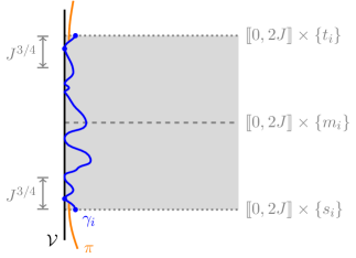
Figure 3. The box $\mathcal{B}_{i}=\llbracket 0,2J\rrbracket\times\llbracket s_{i},t_{i}\rrbracket$ is depicted as a shaded gray square. The polymer $\gamma_{i}$ (blue) hits the initial and final height-$J^{3/4}$ segments of $\mathcal{B}_{i}\cap\mathcal{V}$, and is therefore a local highway: $\gamma_{i}\in\Pi_{i}^{\mathrm{hwy}}$. By definition, the constrained polymer $\pi\sim\mathbb{Q}^{\mathrm{con}}$ (orange) crosses the bottom dotted line segment (height $s_{i}$) between $\mathcal{V}$ and the starting point of $\gamma_{i}$, and similarly $\pi$ crosses the top dotted line segment (height $t_{i}$) between $\mathcal{V}$ and the ending point of $\gamma_{i}$. Planarity entails that $\pi,\gamma_{i}$ intersect within the initial and final strips of height $J^{3/4}=o(J)$, which implies coalescence outside of these strips. In particular, $\pi,\gamma_{i}$ coincide on the dashed midway line $\llbracket 0,2J\rrbracket\times\{m_{i}\}$.

We briefly explain the intuition for Lemma 5.5. By (5.7), the vector $x^{*}=(x_{1}^{*},\dots,x_{N}^{*})$ depends only on the weights inside of $\mathcal{B}\coloneqq\bigcup_{i\in\llbracket 1,N\rrbracket}\mathcal{B}_{i}$. Since the volume $|\mathcal{B}|=o(\sqrt{n})$, the polymer’s behavior within $\mathcal{B}$ is negligible on the diffusive scale. It is therefore probabilistically inexpensive to replace each $(x_{i}^{*},m_{i})$ by a nearby deterministic point, namely $(0,m_{i})$.

Proof of Lemma 5.5.

Let $\pi\sim\mathbb{Q}^{\mathrm{con}}$ and let $\pi^{0}$ be sampled from the conditional measure

$$\pi^{0}\sim\mathbb{Q}^{0}(\cdot)\coloneqq\mathbb{Q}\left(\,\cdot\>|\>\pi^{0}(m_{i})=0\text{ for all }i\in\llbracket 1,N\rrbracket\right).$$

We apply Lemma 2.7 conditionally given the points $\{\pi(m_{i}):i\in\llbracket 1,N\rrbracket\}$ to obtain a coupling $\mathbf{Q}^{\prime}$ of $\mathbb{Q}^{0},\mathbb{Q}^{\mathrm{con}}$ under which $\pi^{0}$ lies to the left of $\pi$ and

$$\pi^{0}\cap\pi\cap\mathcal{H}_{\llbracket m_{i},\;m_{i+1}\rrbracket}\text{ is connected, for all }i\in\llbracket 1,N-1\rrbracket.$$

Our earlier construction of $\mathbf{Q}$ can be lifted along with $\mathbf{Q}^{\prime}$ to a coupling $\mathbf{Q}^{\prime\prime}$ of the measures $\mathbb{Q}^{0},\mathbb{Q}^{\mathrm{con}},\bigotimes_{i\in\llbracket 1,N\rrbracket}\mathbb{Q}_{i}$, i.e. of the triple $(\pi^{0},\pi,(\gamma_{i})_{i\in\llbracket 1,N\rrbracket})$, under which

1. $\pi^{0}$ lies to the left of $\pi$,

2. $\pi$ lies to the left of $\gamma_{i}$ for all $i\in\llbracket 1,N\rrbracket$,

3. $\pi\cap\gamma_{i}$ is connected for all $i\in\llbracket 1,N\rrbracket$, and

4. $\pi^{0}\cap\pi\cap\mathcal{H}_{\llbracket m_{i},\;m_{i+1}\rrbracket}$ is connected for all $i\in\llbracket 1,N-1\rrbracket$.

Fix $\omega\in\mathsf{A}_{2}$. Consider $(\pi^{0},\pi,(\gamma_{i})_{i\in\llbracket 1,N\rrbracket})\sim\mathbf{Q}^{\prime\prime}$. Fix $i\in\llbracket 1,N-1\rrbracket$. By Lemma 5.3,

$$\mathbf{Q}^{\prime\prime}\left(\gamma_{i}\in\Pi_{i}^{\mathrm{hwy}}\quad\text{and}\quad\gamma_{i+1}\in\Pi_{i+1}^{\mathrm{hwy}}\right)=1-o(1).$$ (5.10)

Suppose that $\gamma_{i}\in\Pi_{i}^{\mathrm{hwy}}$ and $\gamma_{i+1}\in\Pi_{i+1}^{\mathrm{hwy}}$. Then by (5.6), planarity, and (Q2), (Q3) (cf. the above proof of Lemma 5.4),

$$\pi\cap\mathcal{V}_{\llbracket t_{i}-J^{3/4},\,\,t_{i}\rrbracket}\neq\varnothing\quad\text{and}\quad\pi\cap\mathcal{V}_{\llbracket s_{i+1},\,\,s_{i+1}+J^{3/4}\rrbracket}\neq\varnothing.$$ (5.11)

Therefore, by planarity and (Q1),

$$\pi^{0}\cap\pi\cap\mathcal{V}_{\llbracket t_{i}-J^{3/4},\,\,t_{i}\rrbracket}\neq\varnothing\quad\text{and}\quad\pi^{0}\cap\pi\cap\mathcal{V}_{\llbracket s_{i+1},\,\,s_{i+1}+J^{3/4}\rrbracket}\neq\varnothing.$$ (5.12)

Moreover, (5.11) implies $\pi(m_{i})=x_{i}^{*}$ and $\pi(m_{i+1})=x_{i+1}^{*}$. We rearrange (5.10) and sum over the possible intersection points in (5.11), (5.12) to conclude that

$$\exp(F_{i}^{0})=(1+o(1))\sum_{a=t_{i}-J^{3/4}}^{t_{i}}\sum_{b=s_{i+1}}^{s_{i+1}+J^{3/4}}Z(0,m_{i},1,a-1)\,Z(0,a,0,b)\,Z(1,b+1,0,m_{i+1}),$$ (5.13)

and that

$$\exp(F_{i}^{*})=(1+o(1))\sum_{a=t_{i}-J^{3/4}}^{t_{i}}\sum_{b=s_{i+1}}^{s_{i+1}+J^{3/4}}Z(x_{i}^{*},m_{i},1,a-1)\,Z(0,a,0,b)\,Z(1,b+1,x_{i+1}^{*},m_{i+1}).$$ (5.14)

By (5.13) and the pigeonhole principle, there exist $a_{i}\in\llbracket t_{i}-J^{3/4},\;t_{i}\rrbracket$ and $b_{i}\in\llbracket s_{i+1},\;s_{i+1}+J^{3/4}\rrbracket$ such that

$$\frac{1}{J^{3/2}}\exp(F^{0}_{i})\lesssim Z(0,m_{i},1,a_{i}-1)\,Z(0,a_{i},0,b_{i})\,Z(1,b_{i}+1,0,m_{i+1}).$$ (5.15)

On the other hand, as the summands in (5.14) are nonnegative, we have

$$\exp(F_{i}^{*})\geq(1+o(1))Z(x_{i}^{*},m_{i},1,a_{i}-1)\,Z(0,a_{i},0,b_{i})\,Z(1,b_{i}+1,x_{i+1}^{*},m_{i+1}).$$ (5.16)

Let us emphasize that the same factor $Z(0,a_{i},0,b_{i})$ appears in (5.15) and (5.16)—this can be interpreted as a manifestation of coalescence, cf. (Q4). Combining (5.15) and (5.16) therefore yields

$$\begin{split}F_{i}^{0}-F_{i}^{*}&\lesssim F(0,m_{i},1,a_{i}-1)+F(1,b_{i}+1,0,m_{i+1})\\ &\quad\quad-F(x_{i}^{*},m_{i},1,a_{i}-1)-F(1,b_{i}+1,x_{i+1}^{*},m_{i+1})+\log J.\end{split}$$

Now by interchanging the roles of $F^{0}_{i}$ and $F^{*}_{i}$ in (5.15) and (5.16), we conclude that

$$\begin{split}|F_{i}^{0}-F_{i}^{*}|&\lesssim F(0,m_{i},1,a-1)+F(1,b+1,0,m_{i+1})\\ &\quad\quad+F(x_{i}^{*},m_{i},1,a^{*}-1)+F(1,b^{*}+1,x_{i+1}^{*},m_{i+1})+\log\log n\end{split}$$ (5.17)

for some $a,a^{*}\in\llbracket t_{i}-J^{3/4},\,\,t_{i}\rrbracket$ and some $b,b^{*}\in\llbracket s_{i+1},\,\,s_{i+1}+J^{3/4}\rrbracket$.

We now observe that the terms on the right side of (5.17) are typically of order $o\left(\sqrt{n}/N\right)$. For instance, we have the deterministic inequality

$$\begin{split}F(0,m_{i},1,a-1)&\leq L(0,m_{i},1,a-1)+\log|\Pi(0,m_{i},1,a-1)|\\ &\leq C(\log n)^{C^{\prime}}\sup_{v\in\mathcal{B}_{i}}\omega(v)+C(\log n)^{C^{\prime}}\end{split}$$ (5.18)

for some absolute constants $C,C^{\prime}$. A union bound and the fact that the weights are subexponential shows that

$$\mathbb{P}\left(\sup_{v\in\mathcal{B}_{i}}\omega(v)>n^{0.01}\right)\leq Ce^{-C^{\prime}n^{0.01}}.$$ (5.19)

Analogous estimates apply to the other terms on the right side of (5.17), and we conclude that there exists an event $\mathsf{B}_{i}$ with

$$\mathbb{P}(\mathsf{B}_{i})\geq 1-Ce^{-C^{\prime}n^{0.01}}\quad\text{and}\quad|F_{i}^{0}-F_{i}^{*}|=o\left(\sqrt{n}/N\right)\text{ on }\mathsf{B}_{i}\cap\mathsf{A}_{2}.$$ (5.20)

As for the case $i\in\{0,N\}$, we note that since $\pi^{0},\pi$ both start at $(0,0)$ and end at $(0,n)$, the coalescence argument above allows us to assume that $\pi^{0},\pi$ coincide on $\mathcal{H}_{\llbracket 0,\,s_{1}\rrbracket}\cup\mathcal{H}_{\llbracket t_{N},\,n\rrbracket}$. This produces a decomposition analogous to (5.13), (5.14), but with the sum over only one intersection point. The rest of the above analysis applies verbatim, and we conclude Lemma 5.5 by combining (5.20) with a union bound over $i\in\llbracket 0,N\rrbracket$. ∎

5.2. Proof of Theorem 5.1: zero temperature

We denote by $\Gamma$ the left-most geodesic $(0,0)\to(0,n)$, and by $\gamma_{i}$ the left-most geodesic $(J^{1/2},s_{i})\to(J^{1/2},t_{i})$, for $i\in\llbracket 1,N\rrbracket$.

By the correspondence of Section 2.5, the proofs of Lemma 5.2 and Lemma 5.3 also imply the analogous zero temperature statements:

Lemma 5.6 (The geodesic is constrained).

There exists an event $\mathsf{E}_{1}$ with $\mathbb{P}(\mathsf{E}_{1})=1-o(1)$, such that $\Gamma\in\Pi^{\mathrm{con}}$ on $\mathsf{E}_{1}$.

Lemma 5.7 (Every geodesic $\gamma_{i}$ is a local highway).

There exists an event $\mathsf{E}_{2}$ with $\mathbb{P}(\mathsf{E}_{2})=1-o(1)$, such that on $\mathsf{E}_{2}$ it holds that $\gamma_{i}\in\Pi_{i}^{\mathrm{hwy}}$ for all $i\in\llbracket 1,N\rrbracket$.

We define

$$x_{0}^{*}\coloneqq 0,\quad x_{N+1}^{*}\coloneqq 0,\quad\text{and}\quad x_{i}^{*}\coloneqq\gamma_{i}(m_{i})\text{ for }i\in\llbracket 1,N\rrbracket,$$

as well as

$$L_{i}^{*}\coloneqq L(x_{i}^{*},m_{i},x_{i+1}^{*},m_{i+1})-\omega(x_{i+1}^{*},m_{i+1})\quad\text{for }i\in\llbracket 0,N-1\rrbracket$$

and $L_{N}^{*}\coloneqq L(x_{N}^{*},m_{N},x_{N+1}^{*},m_{N+1})$. We also write

$$L^{*}\coloneqq\sum_{i=0}^{N}L_{i}^{*},\quad L^{0}\coloneqq\sum_{i=0}^{N}L_{i}^{0},\quad\text{and}\quad L\coloneqq L(0,0,0,n).$$

The zero temperature analogues of Lemma 5.4 and Lemma 5.5 are as follows.

Lemma 5.8.

On $\mathsf{E}_{1}\cap\mathsf{E}_{2}$, we have that $L=L^{*}$.

Lemma 5.9.

As $n\to\infty$,

$$\frac{1}{\sqrt{n}}\left|L^{*}-L^{0}\right|\xrightarrow{\;p\;}0.$$

As with the positive temperature case, Lemma 5.8 and Lemma 5.9 together imply the approximation (5.5), since $\mathbb{P}(\mathsf{E}_{1}\cap\mathsf{E}_{2})=1-o(1)$. Moreover, as Lemma 2.6 trivializes the coupling constructions of Section 5.1, the arguments can be substantially shortened.

Proof of Lemma 5.8.

Fix $\omega\in\mathsf{E}_{1}\cap\mathsf{E}_{2}$. By planarity,

$$\gamma_{i}\cap\Gamma\cap\mathcal{H}_{\llbracket s_{i},\,\,s_{i}+J^{3/4}\rrbracket}\neq\varnothing\quad\text{and}\quad\gamma_{i}\cap\Gamma\cap\mathcal{H}_{\llbracket t_{i}-J^{3/4},\,\,t_{i}\rrbracket}\neq\varnothing\quad\text{for all }i\in\llbracket 1,N\rrbracket.$$

Therefore by Lemma 2.6, $\Gamma(m_{i})=x_{i}^{*}$ for all $i\in\llbracket 0,N+1\rrbracket$. Another application of Lemma 2.6 implies that $L=L^{*}$. ∎

For $i\in\llbracket 0,N\rrbracket$ we denote by $\Gamma_{i}^{0}$ the geodesic $(0,m_{i})\to(0,m_{i+1})$.

Proof of Lemma 5.9.

Fix $\omega\in\mathsf{E}_{1}\cap\mathsf{E}_{2}$. We have $L=L^{*}$ by Lemma 5.8. By planarity,

$$\Gamma_{i}^{0}\cap\Gamma\cap\mathcal{H}_{\llbracket s_{i},\,\,s_{i}+J^{3/4}\rrbracket}\neq\varnothing\quad\text{and}\quad\Gamma_{i}^{0}\cap\Gamma\cap\mathcal{H}_{\llbracket t_{i}-J^{3/4},\,\,t_{i}\rrbracket}\neq\varnothing\quad\text{for all }i\in\llbracket 1,\,N-1\rrbracket,$$

and therefore by Lemma 2.6,

$$\Gamma_{i}^{0}\cap\mathcal{H}_{\llbracket s_{i}+J^{3/4},\,\,t_{i}-J^{3/4}\rrbracket}=\Gamma\cap\mathcal{H}_{\llbracket s_{i}+J^{3/4},\,\,t_{i}-J^{3/4}\rrbracket}\quad\text{for all }i\in\llbracket 1,\,N-1\rrbracket.$$

Similarly,

$$\Gamma_{0}^{0}\cap\mathcal{H}_{\llbracket 0,\,s_{1}\rrbracket}=\Gamma\cap\mathcal{H}_{\llbracket 0,\,s_{1}\rrbracket}\quad\text{and}\quad\Gamma_{N}^{0}\cap\mathcal{H}_{\llbracket t_{N},\,n\rrbracket}=\Gamma\cap\mathcal{H}_{\llbracket t_{N},\,n\rrbracket}.$$

It follows that the symmetric difference $(\Gamma\setminus\Gamma^{0})\cup(\Gamma^{0}\setminus\Gamma)$ is a subset of $\mathcal{B}$, where we define $\Gamma^{0}\coloneqq\bigcup_{i}\Gamma^{0}_{i}$. This implies

$$|L-L^{0}|\leq CN(\log n)^{C^{\prime}}\,\sup_{v\in\mathcal{B}}\omega(v).$$

Lemma 5.9 now follows from (5.19). ∎

6. Fluctuations for free energy with endpoint near the vertical

We make a detour to indicate how the ideas of Lemma 5.5 and Lemma 5.9 can be adapted to prove Corollary 1.10. As discussed in Section 1.2, given Theorem 1.6, the substance of Corollary 1.10 is the approximation

$$\frac{1}{\sqrt{n}}|G(0,0,0,n)-G(0,0,y_{n},n)|\xrightarrow{\;p\;}0\quad\quad\text{whenever}\quad y_{n}=o(\sqrt{n}),$$ (6.1)

which we now establish.

Proof of (6.1).

Assume first $G=F$. Consider polymers $\pi:(0,0)\to(0,n)$ and $\pi^{y}:(0,0)\to(y_{n},n)$, with polymer measures denoted respectively by $\mathbb{Q},\mathbb{Q}^{y}$. As $y_{n}=o(\sqrt{n})$, we can choose $\zeta_{n}\uparrow\infty$ with $w_{n}\coloneqq y_{n}+\zeta_{n}=o(\sqrt{n})$. Theorem 1.4 implies that, for $n$ sufficiently large, there exists an event $\mathsf{B}$ with $\mathbb{P}(\mathsf{B})\geq 0.9$, such that

$$\mathbb{Q}^{y}\left(\pi^{y}\cap\mathcal{V}_{\llbracket n-w_{n},\,\,n-y_{n}\rrbracket}\neq\varnothing\right)\geq 0.99\quad\text{on }\mathsf{B}.$$ (6.2)

Assume the event inside $\mathbb{Q}^{y}$ above occurs. Then by planarity, $\pi$ and $\pi^{y}$ intersect inside the box $\llbracket 0,y_{n}\rrbracket\times\llbracket n-y_{n},n\rrbracket$. The proof of Lemma 5.5 (viz. (5.17)) now implies that for some $a,a^{y}\in\llbracket n-w_{n},\,n-y_{n}\rrbracket$,

$$|F(0,0,0,n)-F(0,0,y_{n},n)|\lesssim F(1,a+1,0,n)+F(1,a^{y}+1,w_{n},n)+\log\zeta_{n}.$$

The arguments of (5.18) and (5.19) imply that the right side above is $o(\sqrt{n})$ with $\mathbb{P}$-probability $1-o(1)$. The case $G=L$ follows by modifying the proof of Lemma 5.9 in an analogous manner. ∎

We now establish the linear growth $\operatorname{Var}(G(0,0,y_{n},n))\asymp n$. The proof of Lemma 4.4 applies verbatim to show $\operatorname{Var}(G(0,0,y_{n},n))\lesssim n$. We prove the lower bound for $G=F$ via a slight modification of the proof of Lemma 4.2 (the same approach works for $G=L$). Fix $j\in\llbracket 0,n-w_{n}\rrbracket$. Recall that in (4.2) we defined

$$\mathsf{A}_{j}\coloneqq\bigl{\{}\omega:\mathbb{Q}(\pi(j)\in\llbracket 0,x_{0}\rrbracket)\geq 0.1\bigr{\}}.$$ (6.3)

Fix $\omega\in\mathsf{A}^{y}_{j}\coloneqq\mathsf{A}_{j}\cap\mathsf{B}$. Let $\mathbf{Q}$ be the coupling of $\mathbb{Q},\mathbb{Q}^{y}$ provided by Lemma 2.7. By planarity and (6.2), the polymers $\pi$ and $\pi^{y}$ are extremely likely to coincide on $\mathcal{H}_{\llbracket 0,\,n-w_{n}\rrbracket}$:

$$\mathbf{Q}\bigl{(}\pi(i)=\pi^{y}(i)\bigr{)}\geq 0.99\quad\text{for all }i\in\llbracket 0,\,n-w_{n}\rrbracket.$$

Therefore by (6.3),

$$\mathbb{Q}^{y}\bigl{(}\pi^{y}(j)\in\llbracket 0,x_{0}\rrbracket\bigr{)}\geq 0.09.$$

As $\mathbb{P}(\mathsf{A}_{j}^{y})\geq 0.8$ and $n-w_{n}\asymp n$, the claimed lower bound $\operatorname{Var}(F(0,0,y_{n},n))\gtrsim n$ now follows from the proof of Lemma 4.2. $\square$

7. Lindeberg condition

In this section we prove Theorem 1.6 by combining the preceding results with the Lindeberg central limit theorem. We recall the latter (see e.g. [Bil95, Theorem 27.2] for a proof):

Theorem 7.1 (Lindeberg central limit theorem).

Let $\{\xi_{N,i}:N\geq 1,\,i\in\llbracket 0,N\rrbracket\}$ be a triangular array, i.e. a collection of random variables such that for any $N$, the random variables $\xi_{N,0},\dots,\xi_{N,N}$ are independent. Suppose that $\mathbb{E}\left[\xi_{N,i}\right]=0$ for all $N,i$ and that $\sum_{i=0}^{N}\operatorname{Var}(\xi_{N,i})=1$ for all $N$. Suppose also that

$$\lim_{N\to\infty}\sum_{i=0}^{N}\mathbb{E}\left[\xi_{N,i}^{2}\,\mathbf{1}_{|\xi_{N,i}|>\varepsilon}\right]=0\quad\text{for all }\varepsilon>0.$$ (7.1)

Then as $N\to\infty$ we have the convergence in distribution

$$\sum_{i=0}^{N}\xi_{N,i}\xrightarrow{\;d\;}\mathsf{N}(0,1).$$

Fix $G\in\{F,L\}$. Let all notation be as in (5.1), (5.2), (5.3), so that $K\asymp n^{0.9}$ and $N\asymp n/K$ and $m_{i+1}-m_{i}\asymp K$ for $i\in\llbracket 0,N-1\rrbracket$ (and $m_{N+1}-m_{N}\lesssim K$). By the variance estimates of Lemma 4.2 and Lemma 4.4, there exists $\sigma_{N}\asymp 1$ such that the triangular array

$$X_{N,i}\coloneqq\frac{G(0,m_{i},0,m_{i+1})-\mathbb{E}\left[G(0,m_{i},0,m_{i+1})\right]}{\sigma_{N}\sqrt{NK}},\quad N\geq 1,\,\,i\in\llbracket 0,N\rrbracket$$

satisfies $\sum_{i=0}^{N}\operatorname{Var}(X_{N,i})=1$ for all $N$. We also have $\mathbb{E}\left[X_{N,i}\right]=0$ for all $N,i$. Finally, we claim that the $X_{N,i}$ also satisfy the Lindeberg condition (7.1):

$$\lim_{N\to\infty}\sum_{i=0}^{N}\mathbb{E}\left[X_{N,i}^{2}\,\mathbf{1}_{|X_{N,i}|>\varepsilon}\right]=0\quad\text{for all }\varepsilon>0.$$ (7.2)

Given (7.2), we can combine Theorem 7.1 with Theorem 5.1 to deduce Theorem 1.6.

Proof of (7.2).

We make a straightforward modification of the proof of the large deviations estimate Lemma 2.1. Fix $N,i$ and write $X\coloneqq X_{N,i}$. Let $\widehat{X}$ denote the same, but with respect to the truncated environment $\widehat{\omega}(x,t)\coloneqq\omega(x,t)\wedge n^{0.04}$. Let $\mathscr{F}_{j}$ be the $\sigma$-algebra generated by $\widehat{\omega}$ up to height $j$, i.e, $\mathscr{F}_{j}\coloneqq\sigma\bigl{(}\widehat{\omega}(x,t):x\in\mathbb{Z}_{\geq 0},\;t\leq j\bigr{)}$. The argument of (2.4) implies that

$$\left|\mathbb{E}\left[\widehat{X}\>|\>\mathscr{F}_{j}\right]-\mathbb{E}\left[\widehat{X}\>|\>\mathscr{F}_{j-1}\right]\right|\leq 2\frac{n^{0.04}}{\sigma_{N}\sqrt{NK}}\leq Cn^{-0.46}\quad\text{for all }j\in\llbracket m_{i},\,m_{i+1}\rrbracket.$$

It follows from the Azuma–Hoeffding inequality that for any $z>0$,

$$\mathbb{P}\left(\bigl{|}\widehat{X}\bigr{|}>z\right)\leq C\exp\left(-C^{\prime}\frac{z^{2}}{(m_{i+1}-m_{i})n^{-0.92}}\right)\leq C\exp\left(-C^{\prime}z^{2}\,n^{0.02}\right).$$

Also, the arguments of (2.7), (2.8) apply verbatim to show that

$$0\leq\mathbb{E}\left[X-\widehat{X}\right]\leq C\exp\left(-C^{\prime}n^{0.02}\right).$$

Fix $\varepsilon>0$. By combining the above two displays with the argument of (2.10), we conclude that there exists $n_{0}>0$ such that for all $n\geq n_{0}$ and for all $z\geq\varepsilon$,

$$\mathbb{P}\bigl{(}|X|>z\bigr{)}\leq C\exp\left(-C^{\prime}\,\min\{1,z^{2}\}\,n^{0.02}\right).$$ (7.3)

It follows that $\mathbb{E}\left[X^{4}\right]=O(1)$. By the Cauchy–Schwarz inequality and another application of (7.3),

$$\mathbb{E}\left[X^{2}\,\mathbf{1}_{|X|>\varepsilon}\right]\leq\mathbb{E}\left[X^{4}\right]^{1/2}\,\mathbb{P}\bigl{(}|X|>\varepsilon\bigr{)}^{1/2}\leq C\exp\left(-C^{\prime}\,\min\{1,\varepsilon^{2}\}\,n^{0.02}\right).$$

Finally, since $n^{0.02}\asymp N^{0.2}$, the above display implies the Lindeberg condition (7.2). ∎

References

- [Abr80] D.. Abraham “Solvable Model with a Roughening Transition for a Planar Ising Ferromagnet” In Phys. Rev. Lett. 44.18, 1980, pp. 1165–1168 DOI: 10.1103/PhysRevLett.44.1165
- [ADH17] Antonio Auffinger, Michael Damron and Jack Hanson “50 years of first-passage percolation”, University Lecture Series Vol. 68 American Mathematical Society, 2017 arXiv:1511.03262
- [BBCS18] Jinho Baik, Guillaume Barraquand, Ivan Corwin and Toufic Suidan “Facilitated Exclusion Process” In Computation and Combinatorics in Dynamics, Stochastics and Control 13 Springer International Publishing, 2018, pp. 1–35 DOI: 10.1007/978-3-030-01593-0˙1
- [BBCS18a] Jinho Baik, Guillaume Barraquand, Ivan Corwin and Toufic Suidan “Pfaffian Schur processes and last passage percolation in a half-quadrant” In Ann. Probab. 46.6, 2018 DOI: 10.1214/17-AOP1226
- [BCD23] Guillaume Barraquand, Ivan Corwin and Sayan Das “KPZ exponents for the half-space log-gamma polymer”, 2023 arXiv:2310.10019
- [BHL83] E. Brézin, B.. Halperin and S. Leibler “Critical Wetting in Three Dimensions” In Phys. Rev. Lett. 50.18, 1983, pp. 1387–1390 DOI: 10.1103/PhysRevLett.50.1387
- [Bil95] Patrick Billingsley “Probability and measure”, Wiley series in probability and mathematical statistics Wiley, 1995
- [BKS03] Itai Benjamini, Gil Kalai and Oded Schramm “First Passage Percolation Has Sublinear Distance Variance” In The Annals of Probability 31.4 Institute of Mathematical Statistics, 2003, pp. 1970–1978 DOI: 10.1214/aop/1068646373
- [Bol82] Erwin Bolthausen “On the Central Limit Theorem for Stationary Mixing Random Fields” In Ann. Probab. 10.4, 1982 DOI: 10.1214/aop/1176993726
- [Bol89] Erwin Bolthausen “A note on the diffusion of directed polymers in a random environment” In Commun.Math. Phys. 123.4, 1989, pp. 529–534 DOI: 10.1007/BF01218584
- [BR01] Jinho Baik and Eric M. Rains “Algebraic aspects of increasing subsequences” In Duke Math. J. 109.1, 2001 DOI: 10.1215/S0012-7094-01-10911-3
- [BR01a] Jinho Baik and Eric M. Rains “The asymptotics of monotone subsequences of involutions” In Duke Math. J. 109.2, 2001 DOI: 10.1215/S0012-7094-01-10921-6
- [BR01b] Jinho Baik and Eric M. Rains “Symmetrized random permutations” In Random Matrix Models and Their Applications, Mathematical Sciences Research Institute publications Vol. 40 Cambridge University Press, 2001 arXiv:math/9910019
- [BSS16] Riddhipratim Basu, Vladas Sidoravicius and Allan Sly “Last Passage Percolation with a Defect Line and the Solution of the Slow Bond Problem”, 2016 arXiv:1408.3464
- [BSS17] Riddhipratim Basu, Sourav Sarkar and Allan Sly “Invariant Measures for TASEP with a Slow Bond”, 2017 arXiv:1704.07799
- [BW23] Guillaume Barraquand and Shouda Wang “An Identity in Distribution Between Full-Space and Half-Space Log-Gamma Polymers” In International Mathematics Research Notices 2023.14, 2023, pp. 11877–11929 DOI: 10.1093/imrn/rnac132
- [CH14] Ivan Corwin and Alan Hammond “Brownian Gibbs property for Airy line ensembles” In Invent. math. 195.2, 2014, pp. 441–508 DOI: 10.1007/s00222-013-0462-3
- [Com17] Francis Comets “Directed Polymers in Random Environments: École d’Été de Probabilités de Saint-Flour XLVI – 2016” 2175, Lecture Notes in Mathematics Springer International Publishing, 2017 DOI: 10.1007/978-3-319-50487-2
- [DHS14] Michael Damron, Jack Hanson and Philippe Sosoe “Subdiffusive concentration in first-passage percolation” In Electron. J. Probab. 19, 2014 DOI: 10.1214/EJP.v19-3680
- [DZ23] Sayan Das and Weitao Zhu “The half-space log-Gamma polymer in the bound phase”, 2023 arXiv:2310.10960
- [GH23] Shirshendu Ganguly and Milind Hegde “Optimal Tail Exponents in General Last Passage Percolation via Bootstrapping & Geodesic Geometry” In Probab. Theory Relat. Fields 186.1, 2023, pp. 221–284 DOI: 10.1007/s00440-023-01204-w
- [Gia07] Giambattista Giacomin “Random Polymer Models” Published by Imperial College Pressdistributed by World Scientific Publishing Co., 2007 DOI: 10.1142/p504
- [HH85] David A. Huse and Christopher L. Henley “Pinning and Roughening of Domain Walls in Ising Systems Due to Random Impurities” In Phys. Rev. Lett. 54.25 American Physical Society, 1985, pp. 2708–2711 DOI: 10.1103/PhysRevLett.54.2708
- [Hol09] Frank Hollander “Random Polymers: École d’Été de Probabilités de Saint-Flour XXXVII – 2007” 1974, Lecture Notes in Mathematics Springer Cham, 2009 DOI: 10.1007/978-3-642-00333-2
- [IL71] I.. Ibragimov and Yu.. Linnik “Independent and stationary sequences of random variables” Wolters-Noordhoff, 1971
- [IMS22] Takashi Imamura, Matteo Mucciconi and Tomohiro Sasamoto “Solvable models in the KPZ class: approach through periodic and free boundary Schur measures”, 2022 arXiv:2204.08420
- [IS88] J.. Imbrie and T. Spencer “Diffusion of directed polymers in a random environment” In J Stat Phys 52.3, 1988, pp. 609–626 DOI: 10.1007/BF01019720
- [Kar85] Mehran Kardar “Depinning by Quenched Randomness” In Phys. Rev. Lett. 55.21 American Physical Society, 1985, pp. 2235–2238 DOI: 10.1103/PhysRevLett.55.2235
- [Kes93] Harry Kesten “On the Speed of Convergence in First-Passage Percolation” In Ann. Appl. Probab. 3.2, 1993 DOI: 10.1214/aoap/1177005426
- [LW09] Quansheng Liu and Frédérique Watbled “Exponential inequalities for martingales and asymptotic properties of the free energy of directed polymers in random environment” In Stochastic Processes and their Applications 119.10, 2009, pp. 3101–3132 DOI: 10.1016/j.spa.2009.05.001
- [NP95] Charles M. Newman and Marcelo S.. Piza “Divergence of Shape Fluctuations in Two Dimensions” In Ann. Probab. 23.3, 1995 DOI: 10.1214/aop/1176988171
- [PSW82] Rahul Pandit, M. Schick and Michael Wortis “Systematics of multilayer adsorption phenomena on attractive substrates” In Phys. Rev. B 26.9, 1982, pp. 5112–5140 DOI: 10.1103/PhysRevB.26.5112