Superhorizon entanglement from inflationary particle production

Abstract

We investigate entanglement generation between the sub- and super-Hubble modes of inflaton fluctuations, in the context of particle production from perturbations during inflation. We consider a large-field inflationary scenario where inflation is driven by a vacuum energy symmetry breaking potential and the scalar inflaton field is nonminimally coupled to spacetime curvature. In particular, we focus on the slow-roll phase, adopting a quasi-de Sitter scale factor to properly account for the presence of perturbations and computing the pair production probability associated to the coupling between the inflaton and spacetime inhomogeneities. The interaction Lagrangian at first order is constructed from inhomogeneities induced by the inflaton dynamics, and the initial Bunch-Davies vacuum state of the field evolves under the action of such Lagrangian. In this framework, we quantify the total amount of entanglement via the von Neumann entropy of the reduced density operator for superhorizon modes, tracing out sub-Hubble degrees of freedom. We then compare these outcomes with entanglement production for quadratic chaotic inflation and for a small-field quadratic hilltop scenario, preserving field-curvature coupling in both cases and pointing out the main differences between large and small-field approaches. We show that the amount of entanglement entropy arising from such geometric production grows rapidly in slow-roll regime and that it is typically higher in large-field scenarios. We also discuss our outcomes in light of recent findings for the squeezing entropy of cosmological perturbations and cubic nonlinearities in de Sitter space.

I Introduction

In recent years, quantum entanglement has been widely recognized as a relevant tool in the context of quantum field theory and gravitation, with important applications spanning from black hole physics bhol and anti-de Sitter/conformal field theory correspondence ads1 ; ads2 ; ads3 , up to de Sitter space dynamics ds1 ; ds2 ; ds3 ; ds4 ; ds5 . In particular, de Sitter space plays a key role in modeling the very early universe evolution, since a primordial phase of strong acceleration known as inflation infl1 ; infl2 ; infl3 has been proposed to solve the main issues related to the standard Big Bang paradigm wein ; uzan .

All successful inflationary models should properly deal with the quantum fluctuations of all fields involved, which are thought to be the fundamental seeds for structure formation in our universe pert1 ; pert2 . Such fluctuations are typically studied in Fourier space: to leading order, each Fourier mode evolves independently, obeying a harmonic oscillator equation with time-dependent mass. The Hubble horizon then emerges as a natural scale to describe the dynamics of inflaton fluctuations, which typically oscillate in time on sub-Hubble scales, while becoming frozen on super-Hubble ones rio .

The corresponding quantum-to-classical transition of inflaton fluctuations, i.e., how short wavelength quantum fluctuations are stretched by cosmic expansion and lose their quantum nature, is not yet fully understood, although some headway has been made in the last decades by investigating the effects of squeezing and decoherence sq1 ; sq2 ; sq3 ; sq4 ; sq5 ; sq6 ; dec1 ; dec2 ; dec3 ; dec4 ; dec5 ; meas1 ; meas2 , also resorting in some cases to open quantum system techniques. Recently, the decoherence mechanism for scalar inflaton fluctuations has been revised by taking into account the role of cubic non-Gaussianities brand20 . Specifically, due to the nonlinear nature of Einstein equations, it was argued that a certain amount of mode-mixing for cosmological perturbations is always present. This implies a mixing between the sub- and super-Hubble modes, which leads to decoherence of the reduced density matrix of each subsystem. Interestingly, such nonlinearities seem to produce the most relevant contribution to the entropy of cosmological perturbations, surpassing the entropy associated to the squeezed vacuum (see also bra92 ; bra93 ; gasp1 ; gasp2 ). In other words, the entanglement entropy due to cubic interactions dominates over the one due to the (quadratic) squeezing Hamiltonian, provided inflation lasts for a sufficiently long period of time, in agreement with observations planck .

Cubic interactions of density perturbations provide us with a lower bound on the amount of entanglement entropy for scalar perturbations. Indeed, such gravitational nonlinearities are inevitably present in most inflationary models. The corresponding entanglement is usually quantified by means of the von Neumann entropy for the reduced density operator corresponding to super-Hubble modes. However, in recent years it was argued that inflationary particle production may work as a noise and affect entanglement generation across the Hubble scales oqs7 .

Motivated by the above picture, we here investigate the dynamics of superhorizon entanglement associated with geometric particle production fri ; ces in a single-field inflationary scenario. Geometric production during inflation is typically studied resorting to a perturbative approach, where the presence of spacetime inhomogeneities is traced back to the quantum fluctuations of the inflaton field and the interacting Lagrangian is constructed by coupling metric perturbations to the energy-momentum tensor of a given quantum field. In particular, the energy-momentum tensor for the inflationary fluctuations of a scalar field has been considered in bel1 , showing that geometric production may lead to a non-negligible amount of entanglement for particle pairs on super-Hubble scales. Here we extend this approach by studying entanglement entropy generation across the horizon, during the slow-roll regime. We adopt the usual momentum-space entanglement techniques proposed in msent1 ; msent2 ; msent3 and then generalized to de Sitter space in lel ; msent4 , focusing on the pair production probability arising from scalar spacetime perturbations. In so doing, we start from a large-field model of inflation driven by a symmetry breaking potential transporting vacuum energy, also including a nonminimal coupling term between the inflaton field and the scalar spacetime curvature. We compute the von Neumann entropy associated to the reduced density operator for super-Hubble modes and we then compare these outcomes with the widely-studied chaotic quadratic potential qchaos1 ; qchaos2 ; qchaos3 and the small-field quadratic hilltop one hill1 ; hill2 , preserving in both cases the nonminimal coupling term with the scalar curvature. For large-field models, we will show that the total amount of entanglement at the end of the slow-roll phase is typically non-negligible. This implies that particle production during the inflationary regime may significantly alter the process of entanglement generation for inflaton fluctuations. Last but not least, we discuss the scale-dependence of entanglement entropy, which represents a peculiar issue of momentum-space calculations. In particular, an ultraviolet (UV) cutoff scale associated with the Planck mass $M_{\rm pl}$ is required, and we also debate limitations on the infrared (IR) scales.

This work is organized as follows. In Sec. II, we introduce the nonminimally coupled scalar inflaton field and its quantum fluctuations. In Sec. III, we review the mechanism of particle production from inhomogeneities. In Sec. IV, we quantify the superhorizon entanglement generated in this process, obtaining the von Neumann entropy associated with super-Hubble modes and comparing these outcomes with a quadratic chaotic model and a small-field quadratic hilltop scenario. We also discuss our main findings and compare our approach with previous studies. Finally, Sec. V is devoted to conclusions and perspectives. We use natural units $c=\hbar=1$ throughout the paper.

II Inflationary warm up

We consider a scalar inflaton field $\phi$, nonminimally coupled to the scalar curvature of spacetime $R$. The corresponding Lagrangian density is written as

$$\mathcal{L}=\frac{1}{2}\left[g^{\mu\nu}\phi_{,\mu}\phi_{,\nu}-\xi R\phi^{2}\right]-V(\phi),$$ (1)

where $\xi$ is the field-curvature coupling constant and the potential $V(\phi)$ is left unspecified for the moment. The universe expansion during inflation can be modeled by a spatially flat Friedmann-Robertson-Walker background, whose line element in cosmic time $t$ reads $ds^{2}=dt^{2}-a^{2}(t)d{\bf x}^{2}$.

As usual, we introduce conformal time $\tau=\int dt/a(t)$ in order to simplify the dynamics of the inflaton field during slow-roll rio ; brand20 . In particular, we can write the unperturbed metric tensor as $g_{\mu\nu}=a^{2}(\tau)\eta_{\mu\nu}$, where $\eta_{\mu\nu}$ is the Minkowski tensor.

In conformal time, introducing the effective potential,

$$V^{\rm eff}(\phi,R)\equiv V(\phi)+\frac{1}{2}\xi R\phi^{2},$$ (2)

the zero-order equation of motion for the inflaton field takes the form

$$\frac{1}{\sqrt{-g}}\partial_{\mu}\left(\sqrt{-g}g^{\mu\nu}\partial_{\nu}\phi\right)+V^{\rm eff}_{,\phi}=0,$$ (3)

with $V^{\rm eff}_{,\phi}\equiv\partial V(\phi)/\partial\phi$ and $g$ is the determinant of the metric tensor.

II.1 Inflaton quantum fluctuations

We now introduce quantum fluctuations in the above framework. We start by considering the usual ansatz for the inflaton field rio ; bel1

$$\phi({\bf x},\tau)=\phi_{0}(\tau)+\delta\phi({\bf x},\tau),$$ (4)

where the background homogeneous contribution $\phi_{0}$ has been isolated from the perturbing quantum fluctuations $\delta\phi$. The most general metric tensor describing scalar perturbations to linear order can be expressed in the form

$$g_{\mu\nu}=a^{2}(\tau)\begin{pmatrix}(1+2\Phi)&\partial_{i}B\\ \partial_{i}B&-\left((1-2\Psi)\delta_{ij}+D_{ij}E\right)\\ \end{pmatrix},$$ (5)

where $\Phi$, $\Psi$, $B$ and $E$ are scalar quantities and $D_{ij}\equiv\partial_{i}\partial_{j}-\frac{1}{3}\delta_{ij}\nabla^{2}$.

Hereafter, we adopt the longitudinal, or conformal Newtonian gauge, equivalent to set $E=B=0$. Moreover, when the fluctuation matter source has no anisotropic stress, as for the scalar inflaton, we can further set $\Phi=\Psi$. In Fourier space, we write perturbation modes as pert1

$$\Psi({\bf x},\tau)=\Psi_{k}(\tau)e^{i{\bf k}\cdot{\bf x}},$$ (6)

and, similarly, we can expand quantum fluctuations as

$$\hat{\delta\phi}({\bf x},\tau)=\frac{1}{(2\pi)^{3/2}}\int d^{3}k\left(\hat{a}_{k}\delta\phi_{k}e^{i{\bf k}\cdot{\bf x}}+\hat{a}_{k}^{\dagger}\delta\phi_{k}^{*}e^{-i{\bf k}\cdot{\bf x}}\right),$$ (7)

satisfying the usual canonical commutation relations, $[\hat{a}_{k},\hat{a}_{k^{\prime}}^{\dagger}]=\delta^{(3)}({\bf k}-{\bf k^{\prime}})$.

Following Refs. rio ; bel1 and dropping the subscript $0$ for clearness, the first-order perturbed equations become

$$\delta\phi_{k}^{\prime\prime}+2\mathcal{H}\delta\phi_{k}^{\prime}+k^{2}\delta\phi_{k}-4\Psi_{k}^{\prime}\phi^{\prime}$$

$$=-\xi\left(-2k^{2}\Psi_{k}-6\Psi_{k}^{\prime\prime}-24\mathcal{H}\Psi_{k}^{\prime}-12\frac{a^{\prime\prime}}{a}\Psi_{k}\right)\phi$$

$$\ \ \ -\left(V^{\rm eff}_{,\phi\phi}\delta\phi_{k}+2\Psi_{k}V^{\rm eff}_{,\phi}\right)a^{2},$$ (8)

where the prime denotes derivatives with respect to conformal time and $\mathcal{H}\equiv a^{\prime}/a$. If $\lvert\xi\rvert\ll 1$, we can exploit the slow-roll condition and the $(0,i)$ component of perturbed Einstein’s equations

$$\Psi_{k}^{\prime}+\mathcal{H}\Psi_{k}=\epsilon\mathcal{H}^{2}\frac{\delta\phi_{k}}{\phi^{\prime}},$$ (9)

where $\epsilon$ is a slow-roll parameter specified later on, to simplify Eq. (II.1) as

$$\delta\phi_{k}^{\prime\prime}+2\mathcal{H}\delta\phi_{k}^{\prime}+\left[k^{2}+V^{\rm eff}_{,\phi\phi}a^{2}+6\epsilon\mathcal{H}^{2}\right]\delta\phi_{k}=0.$$ (10)

II.2 Inflaton modes in a quasi-de Sitter background

As mentioned in Sec. I, inflation leads to a de Sitter phase during which the universe experiences a period of intense acceleration. However, the inflationary epoch cannot precisely manifest an exact de Sitter phase, since small deviations are inevitably present as consequence of the inflaton dynamics. To accomplish these slight deviations, we here adopt a quasi-de Sitter background evolution rio

$$a(\tau)=-\frac{1}{H_{I}\tau^{(1+\epsilon)}},\ \ \ \ \epsilon\ll 1,$$ (11)

where $\tau<0$ and $H_{I}$ is the Hubble parameter during inflation, while $\epsilon$ can be identified as a small and constant slow-roll parameter.

Inserting Eq. (11) into Eq. (10) and rescaling the field by $\delta\chi_{k}=\delta\phi_{k}a$, we obtain

$$\delta\chi_{k}^{\prime\prime}+\left[k^{2}-\frac{1}{\tau^{2}}\left(\left(1-6\xi\right)(2+3\epsilon)+6\epsilon-\frac{V^{\rm eff}_{\phi\phi}}{H_{I}^{2}}\right)\right]\delta\chi_{k}=0,$$ (12)

where we also computed the scalar curvature in conformal time, $R=6a^{\prime\prime}/a^{3}$, and noted that $a^{\prime\prime}/a\simeq(2+3\epsilon)/\tau^{2}$. Eq. (12) admits solutions

$$\delta\chi_{k}(\tau)=\sqrt{-\tau}\left[c_{1}(k)H_{\nu}^{(1)}(-k\tau)+c_{2}(k)H_{\nu}^{(2)}(-k\tau)\right],$$ (13)

where $H_{\nu}^{(1)}$ and $H_{\nu}^{(2)}$ are Hankel functions and

$$\nu=\sqrt{\frac{1}{4}+(1-6\xi)(2+3\epsilon)+6\epsilon-V^{\rm eff}_{,\phi\phi}/H_{I}^{2}}.$$ (14)

The integration constants $c_{1}(k)$ and $c_{2}(k)$ can be determined by choosing the state of the field when inflation starts. A common ansatz consists in employing the Bunch-Davies vacuum state bunch1 ; bunch2 ; bunch3 , that corresponds to impose the boundary condition

$$\delta\chi_{k}\xrightarrow[\tau\rightarrow-\infty]{}\frac{e^{-ik\tau}}{\sqrt{2k}}.$$ (15)

This choice implies $c_{1}(k)=\sqrt{\pi}e^{i(\nu+\frac{1}{2})\frac{\pi}{2}}/2$ and $c_{2}(k)=0$, so the original fluctuation modes take the form

$$\delta\phi_{k}(\tau)=\frac{\sqrt{-\pi\tau}}{2}e^{i\left(\nu+\frac{1}{2}\right)\frac{\pi}{2}}H^{\left(1\right)}_{\nu}\left(-k\tau\right)/a(\tau).$$ (16)

Our primary focus will be to compute entanglement between sub- and super-Hubble modes. Thus, we exploit the asymptotic behavior of Hankel functions

$$H^{\left(1\right)}_{\nu}\left(x\gg 1\right)\simeq\sqrt{\frac{2}{\pi x}}e^{i\left(x-\frac{\pi}{2}\nu-\frac{\pi}{4}\right)},$$ (17)

$$H^{\left(1\right)}_{\nu}\left(x\ll 1\right)\simeq\sqrt{\frac{2}{\pi}}e^{-i\frac{\pi}{2}}2^{\left(\nu-\frac{3}{2}\right)}\frac{\Gamma\left(\nu\right)}{\Gamma\left(\frac{3}{2}\right)}x^{-\nu}$$ (18)

to derive the expressions for fluctuations inside and outside the comoving Hubble radius $r_{H}(\tau)=1/(a(\tau)H_{I})$. We then introduce

$${\emph{ Sub-Hubble\,\,scales}:}$$

$$\delta\phi_{k}^{\rm sub}\simeq\frac{1}{\sqrt{2k}}\frac{e^{i\left(\nu+\frac{1}{2}\right)\frac{\pi}{2}}\ e^{i\left(-k\tau-\frac{\pi}{2}\nu-\frac{\pi}{4}\right)}}{a(\tau)},$$ (19)

$${\emph{ Super-Hubble\,\,scales}:}$$

$$\delta\phi_{k}^{\rm super}\simeq e^{i\left(\nu-\frac{1}{2}\right)\frac{\pi}{2}}2^{\left(\nu-\frac{3}{2}\right)}\frac{\Gamma\left(\nu\right)}{\Gamma\left(\frac{3}{2}\right)}\frac{H_{I}}{\sqrt{2k^{3}}}\left(\frac{k}{aH_{I}}\right)^{\frac{3}{2}-\nu}.$$ (20)

Remarkably, we notice that fluctuations oscillate on sub-Hubble scales, $k\gg aH_{I}$, while being nearly frozen after crossing the horizon. Later on, we will specify these calculations to some relevant inflationary potentials, in order to derive the dynamics of the corresponding inflaton fluctuations and quantify entanglement generation during the slow-roll phase. First, we briefly recall the mechanism of particle production from inhomogeneities during inflation.

III Geometric particle production

Particle production from spacetime inhomogeneities has been proposed some time ago fri ; ces as an alternative mechanism to the widely-studied GPP scenario. More precisely,

• the presence of space-dependent perturbations in an expanding background is expected to enhance the total amount of particles produced,

• such perturbations break the space translation symmetry bel2 and, accordingly, “geometric” production is not limited to pair production with opposite momenta.

Assuming a perturbed background, with

$$g_{\mu\nu}=a^{2}(\tau)\left(\eta_{\mu\nu}+h_{\mu\nu}\right),\ \ \ \ \lvert h_{\mu\nu}\rvert\ll 1,$$ (21)

we can write the first-order interaction Lagrangian density describing the coupling between perturbations and a given quantum field in the form

$$\mathcal{L}_{I}=-\frac{1}{2}\sqrt{-g_{(0)}}H^{\mu\nu}T^{\left(0\right)}_{\mu\nu},$$ (22)

where $T_{\mu\nu}^{(0)}$ is the zero-order energy-momentum tensor for the field, $g_{(0)}$ the determinant of the background unperturbed metric tensor and $H_{\mu\nu}=a^{2}(\tau)h_{\mu\nu}$. In the longitudinal gauge, scalar perturbations associated with $\phi$ take the simple form

$$h_{\mu\nu}=\begin{pmatrix}2\Psi&0&0&0\\ 0&2\Psi&0&0\\ 0&0&2\Psi&0\\ 0&0&0&2\Psi\\[4.5pt] \end{pmatrix}.$$ (23)

The perturbation potential $\Psi$ is derived from Eq. (9), which can be recast in the form

$$\Psi_{k}^{\prime\prime}+2\left(\mathcal{H}-\frac{\phi^{\prime\prime}}{\phi^{\prime}}\right)\Psi_{k}^{\prime}+2\left(\mathcal{H}^{\prime}-\mathcal{H}\frac{\phi^{\prime\prime}}{\phi^{\prime}}\right)+k^{2}\Psi_{k}=0,$$ (24)

where we also exploited the mode decomposition of Eq. (6). Moreover, since we focus on the dynamics of inflaton fluctuations, we assume

$$T_{\mu\nu}^{(0)}= \partial_{\mu}\delta\phi\ \partial_{\nu}\delta\phi-\frac{1}{2}g_{\mu\nu}^{(0)}\left[g^{\rho\sigma}_{(0)}\ \partial_{\rho}\delta\phi\ \partial_{\sigma}\delta\phi-V(\delta\phi)\right]$$

$$-\xi\left[\nabla_{\mu}\partial_{\nu}-g_{\mu\nu}^{(0)}\nabla^{\rho}\nabla_{\rho}+R_{\mu\nu}^{(0)}-\frac{1}{2}R^{(0)}g_{\mu\nu}^{(0)}\right](\delta\phi)^{2}.$$ (25)

Introducing now the interaction Hamiltonian density as $\mathcal{H}_{I}$, it can be shown that $\mathcal{L}_{I}=-\mathcal{H}_{I}$ holds for a Lagrangian density of the form (22). This implies that we can write the $S$ matrix at first-order in Dyson’s expansion as

$$\hat{S}\simeq 1+i\hat{T}\int d^{4}x\mathcal{L}_{I}.$$ (26)

We will focus on particle pair production for inflationary potentials of the form $V\propto\phi^{2n}$ ($n=1,2$). The corresponding probability amplitude for pair creation reads

$$\mathcal{C}_{{\bf p}_{1},{\bf p}_{2}} \equiv\langle{\bf p}_{1},{\bf p}_{2}\lvert\hat{S}\rvert 0\rangle$$

$$=-\frac{i}{2}\int d^{4}x\ 2a^{2}\big{(}A_{0}({\bf x},\tau)+A_{1}({\bf x},\tau)$$

$$\ \ \ \ \ \ \ \ \ \ \ \ \ \ \ \ \ \ \ \ \ \ \ \ \ \ +A_{2}({\bf x},\tau)+A_{3}({\bf x},\tau)\big{)},$$ (27)

where

$$A_{0}({\bf x},\tau)=2\Psi\bigg{[} \partial_{0}\delta\phi_{p_{1}}^{*}\ \partial_{0}\delta\phi_{p_{2}}^{*}$$

$$-\frac{1}{2}\big{(}\eta^{\rho\sigma}\partial_{\rho}\delta\phi_{p_{1}}^{*}\ \partial_{\sigma}\delta\phi_{p_{2}}^{*}-a^{2}V(\delta\phi)\big{)}$$

$$-\xi\bigg{(}\partial_{0}\partial_{0}-\frac{a^{\prime}}{a}\partial_{0}-\eta^{\rho\sigma}\partial_{\rho}\partial_{\sigma}$$

$$\ \ \ \ \ \ \ -3\left(\frac{a^{\prime}}{a}\bigg{)}^{2}\right)\delta\phi_{p_{1}}^{*}\delta\phi_{p_{2}}^{*}\bigg{]}e^{-i({\bf p_{1}}+{\bf p_{2}})\cdot{\bf x}}$$

and

$$A_{i}({\bf x},\tau)=2\Psi\bigg{[} \partial_{i}\delta\phi_{p_{1}}^{*}\ \partial_{i}\delta\phi_{p_{2}}^{*}$$

$$+\frac{1}{2}\big{(}\eta^{\rho\sigma}\partial_{\rho}\delta\phi_{p_{1}}^{*}\ \partial_{\sigma}\delta\phi_{p_{2}}^{*}-a^{2}V(\delta\phi)\big{)}$$

$$-\xi\bigg{(}\partial_{i}\partial_{i}+\frac{3a^{\prime}}{a}\partial_{0}+\frac{2a^{\prime\prime}}{a}+\eta^{\rho\sigma}\partial_{\rho}\partial_{\sigma}$$

$$\ \ \ \ \ \ \ \ -\left(\frac{a^{\prime}}{a}\right)^{2}\bigg{)}\delta\phi_{p}^{*}\delta\phi_{q}^{*}\bigg{]}e^{-i({\bf p_{1}}+{\bf p_{2}})\cdot{\bf x}},$$

for $i=1,2,3$. For each particle pair, the final state can be written in the form

$$\lvert\Psi\rangle=\hat{S}\lvert 0_{{\bf p}_{1}};0_{{\bf p}_{2}}\rangle=\mathcal{N}\left(\lvert 0_{{\bf p}_{1}};0_{{\bf p}_{2}}\rangle+\frac{1}{2}\mathcal{C}_{{\bf p}_{1},{\bf p}_{2}}\lvert 1_{{\bf p}_{1}};1_{{\bf p}_{2}}\rangle\right),$$ (30)

where the normalization factor $\mathcal{N}$ is derived as usual by imposing $\langle\Psi\rvert\Psi\rangle=1$. The total number density of particles arising from the interacting Lagrangian, Eq. (22), at second perturbative order is then

$$N^{(2)}(\tau)=\frac{a^{-3}(\tau)}{\left(2\pi\right)^{3}}\int d^{3}p_{1}\ d^{3}p_{2}\ \lvert\mathcal{C}_{{\bf p}_{1},{\bf p}_{2}}\rvert^{2}$$

$$\times\left(1+\lvert\beta_{p_{1}}\rvert^{2}+\lvert\beta_{p_{2}}\rvert^{2}\right).$$ (31)

In Eq. (III), we introduced the Bogoliubov coefficients $\beta_{p_{1}}$ and $\beta_{p_{2}}$, which can be derived from the dynamics of the field modes $\delta\phi_{k}$ in the asymptotic regions $\tau\rightarrow\pm\infty$. It can be shown that Bogoliubov coefficients are zero in a purely de Sitter spacetime gpp2 , while in the context of GPP they can be computed assuming a rapid transition from inflation to the radiation dominated era gpp10 ; boya . In these models, the quasi de Sitter scale factor of Eq. (11) should be modified in order to guarantee a continuous transition between the two epochs, thus avoiding divergences. The process of gravitational production is more effective during the nonadiabatic inflationary expansion of the universe, while adiabaticity is gradually recovered before matter radiation equality, so that a proper definition of particle states is again possible at sufficiently large $\tau$. Bogoliubov coefficients can also describe the squeezing of cosmological perturbations during inflation brand20 ; bra92 ; bra93 ; gasp1 ; gasp2 , even if this approach has been recently criticized due to possible ambiguities that may arise in defining squeezed states for quantum fields in expanding backgrounds sq6 . We will return to this issue in Sec. IV.2, while in the following we are going to compute superhorizon entanglement associated to geometric particle production during the slow-roll phase of inflation. From now on, we will neglect the contribution of Bogoliubov coefficients to particle creation from inhomogeneities, thus focusing on the pure geometric contribution described by the probability amplitude of Eq. (III).

IV Superhorizon entanglement entropy

The degrees of freedom of any interacting quantum field theory are entangled in momentum space msent1 . In particular, inflationary perturbations are mostly studied in momentum space, as the properties of momentum modes are typically probed in experimental contexts planck .

Specifically, during inflation the (comoving) Hubble radius $r_{H}$ naturally divides the total Hilbert space of states into sub-Hubble and super-Hubble subspaces, respectively brand20 . This implies that the entanglement entropy of inflaton fluctuations can be identified as the von Neumann entropy associated with the reduced density matrix of one of these two subsystems.

Given the generic probability amplitude for particle production up to the first order in $h$,

$$\mathcal{C}_{n,N}=\langle n,N\lvert\left(-i\int_{\tau_{0}}^{\tau}d\tau^{\prime}\mathcal{H}_{I}(\tau^{\prime})\right)\rvert 0,0\rangle+\mathcal{O}(h^{2}),$$ (32)

where $n$ is the number of particles in the subsystem traced out and $N$ the particles in the main system, we can write the von Neumann entropy of the reduced state as

$$\mathcal{S}_{\rm ent}=-\sum_{n,N\neq 0}\lvert\mathcal{C}_{n,N}\rvert^{2}\left(\ln\ \lvert\mathcal{C}_{n,N}\rvert^{2}-1\right)+\mathcal{O}(h^{3}).$$ (33)

This result can be re-expressed in momentum space by the substitution $\sum_{n,N\neq 0}\rightarrow\sum_{\{{\bf p}_{i}\}\gtrless\mu}$, where $\mu$ stands for a generic momentum cutoff scale, obtaining the following entropy per unitary volume

$$\mathcal{S}_{\rm ent}= -\int_{\{{\bf p}_{i}\}\gtrless\mu}\prod_{i}^{d}d^{3}p_{i}\left[\lvert\mathcal{C}_{\{{\bf p}_{i}\}\gtrless\mu}\rvert^{2}\left(\ln\ \lvert\mathcal{C}_{\{{\bf p}_{i}\}\gtrless\mu}\rvert^{2}-1\right)\right]$$

$$+\mathcal{O}(h^{3}).$$ (34)

In case of entanglement associated with inflationary fluctuations, the Hubble radius is the natural separation scale for field modes. Hence, we can set $\mu\equiv r_{H}(\tau)$ in order to compute entanglement across the Hubble horizon. Moreover, one usually assumes the space of super-Hubble modes to be the system under analysis, while the sub-Hubble space is treated as the “bath” we integrate over.

Focusing now on perturbative particle production from inhomogeneities, we are interested in amplitudes of the form

$$\mathcal{C}_{\{{\bf p}_{i}\}}=\langle{\bf p}_{1}{\bf p}_{2}\lvert\left(i\int_{\tau_{0}}^{\tau}d\tau^{\prime}\mathcal{L}_{I}(\tau^{\prime})\right)\rvert 0,0\rangle+\mathcal{O}(h^{2}),$$ (35)

where $\mathcal{L}_{I}$ is given by Eq. (22) and we are focusing on quadratic terms only.

In our treatment, the total amount of superhorizon entanglement is thus obtained by picking one mode on super-Hubble scales and the other on sub-Hubble ones, namely

$$\{{\bf p}_{i}\}=\begin{cases}a(\tau_{i})H_{I}<\lvert{\bf p}_{1}\rvert<a(\tau)H_{I},\\ a(\tau)H_{I}<\lvert{\bf p}_{2}\rvert<a(\tau)M_{\rm pl}.\end{cases}$$ (36)

In Eq. (36), we introduced the usual UV cutoff for comoving momenta in terms of the Planck mass, $M_{\rm pl}$. At the same time, our IR cutoff consists in neglecting all modes whose wavelength exceeds the Hubble radius at the beginning of inflation. Consequently, with this choice all super-Hubble modes are created during the quasi-de Sitter expansion, thus allowing a causal generation mechanism for cosmological perturbations brand20 .

In the following, we specify the here-presented approach to some relevant inflationary potentials.

IV.1 Choosing the inflationary potentials

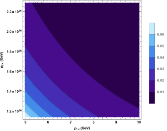
Figure 1: Superhorizon entanglement entropy $\mathcal{S}_{\rm ent}$ at time $\tau_{f}$ from geometric particle production, assuming a quartic self-coupling inflationary potential. The entropy is plotted as function of the super-Hubble mode $p_{1x}$ and the sub-Hubble mode $p_{2x}$. The other momentum components are set to zero, for simplicity. We assume $\phi(\tau_{i})=5$ $M_{\rm pl}$, $\lambda=10^{-15}$, $\epsilon=10^{-3}$, $\xi=10^{-4}$ and $\tau^{*}=\tau_{0}/1000=-10^{-3}$ GeV^-1.

Recent results from the Planck satellite have imposed stringent constraints on the potentials that can be feasibly adopted to drive the inflationary epoch planck . Power-law potentials, in particular, seem to be disfavored by observations, albeit the curvature coupling seems to resort their use in inflationary stages. Analogously, chaotic and hilltop potentials still appear to be plausible options to describe inflation. Motivated by these results, in order to quantify superhorizon entanglement arising from geometric particle production, we focus on three specific potentials, as discussed below.

• We start from a quartic self-coupling interaction, selecting the potential

  $$V(\phi)=\frac{\lambda}{4}\left(\phi^{2}-v^{2}\right)^{2},$$ (37)

  where $v$ is the vacuum expectation value of the inflaton field. Inflationary predictions associated to a nonminimal quartic potential have been studied in detail, see e.g. qchaos2 ; qchaos3 ; tsuqua . Moreover, this potential has been recently proposed in the context of vacuum energy cancellation during inflation carl .

  In a large-field scenario, we can safely set $V(\phi)\simeq\lambda\phi^{4}/4$ during slow-roll. Accordingly, the slow-roll background equation for the inflaton field can be expressed in conformal time as

  $$3\mathcal{H}\phi^{\prime}=-\left(\lambda\phi^{3}+\xi R\phi\right)a^{2},$$ (38)

  that, for a quasi-de Sitter evolution, gives

  $$\phi^{\prime}-\frac{3\xi(2+3\epsilon)}{(1+\epsilon)\tau}\phi=\frac{\lambda}{2(1+\epsilon)H_{I}^{2}\tau}\phi^{3}.$$ (39)

  Eq. (39) is solved resorting to the usual techniques for Bernoulli differential equations.

  Once derived the background dynamics, we can obtain the fluctuation modes for the inflaton field. For simplicity, during slow-roll we make the substitution

  $$\phi^{2}\rightarrow\frac{\int_{\tau_{i}}^{\tau_{f}}\phi^{2}d\tau}{\tau_{f}-\tau_{i}}\equiv\langle\phi^{2}\rangle,$$ (40)

  thus identifying $\phi^{2}$ with its mean value. The final time $\tau_{f}$ is usually determined by imposing a number $N_{\rm tot}$ of e-foldings which is sufficient to solve the horizon and flatness problems, e.g.

  $$N_{\rm tot}=\int dtH(t)\simeq-\int_{\tau_{i}}^{\tau_{f}}d\tau/\tau=60.$$ (41)

  Exploiting now Eqs. (39)-(40), the solution for inflaton fluctuations is in the form (16), with

  $$\ \ \ \ \ \ \ \ \nu\simeq\sqrt{\frac{1}{4}+(1-6\xi)(2+3\epsilon)+6\epsilon-3\lambda\langle\phi^{2}\rangle/H_{I}^{2}}.$$ (42)

  When dealing with quartic terms, we are interested in probability amplitudes of the form

  $$\mathcal{C}_{{\bf p}_{1},{\bf p}_{2}} \propto\langle{\bf p}_{1},{\bf p}_{2}\lvert\hat{T}\left[(\delta\phi)^{4}\right]\rvert 0\rangle$$

  $$=12\ \delta\phi_{p_{1}}^{*}({\bf x},\tau)\delta\phi_{p_{2}}^{*}({\bf x},\tau)G_{F}\langle 0\rvert 0\rangle,$$ (43)

  where $\hat{T}$ is the time-ordering operator and $\lvert 0\rangle$ denotes the Bunch-Davies initial vacuum state. Such amplitudes clearly diverge, due to the presence of the Feynman propagator $G_{F}$ and, so, the need of renormalizing self-interacting scalar field theories in curved spacetime is crucial.

  Hence, cancelling poles in the amplitudes requires appropriate rescaling of the coupling constants. For example, by setting

  $$\xi_{R}=\xi-\delta\xi,$$ (44a)

  $$\lambda_{R}=\lambda-\delta\lambda,$$ (44b)

  where $\xi_{R}$ and $\lambda_{R}$ are renormalized constants, we obtain

  $$\ \ \ \ \ \langle{\bf p}_{1},{\bf p}_{2} \lvert\hat{T}\left[(\delta\phi)^{4}\right]\rvert 0\rangle_{\rm ren}\propto\ \delta\phi_{p_{1}}^{*}({\bf x},\tau)\delta\phi_{p_{2}}^{*}({\bf x},\tau)$$

  $$\ \ \ \ \ \ \ \ \times\left\{G_{F}^{\rm fin}+\frac{i}{8\pi^{2}}\left(\xi_{R}-\frac{1}{6}\right)R\ln\mu\right\}.$$ (45)

  In Eq. (- ‣ IV.1), the propagator $G_{F}^{\rm fin}$ is finite in four dimensions gpp2 , while $\mu$ is an arbitrary mass scale. Rescaling of $\mu$ simply readjusts the relations between bare and renormalized constants, thus implying that measurements are required to fix the $\lambda_{R}$ and $\xi_{R}$ magnitudes.
  

  

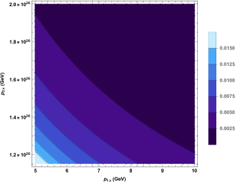
  Figure 2: Superhorizon entanglement entropy $\mathcal{S}_{\rm ent}$ at time $\tau_{f}$ from geometric particle production, assuming a quadratic chaotic potential. The entropy is plotted as function of the super-Hubble mode $p_{1x}$ and the sub-Hubble mode $p_{2x}$. The other momentum components are set to zero, for simplicity. We assume $\phi(\tau_{i})=5$ $M_{\rm pl}$, $\epsilon=10^{-3}$, $\xi=10^{-4}$ and $\tau^{*}=\tau_{0}/1000=-10^{-3}$ GeV^-1. Moreover, the mass of the field is $m=1.34\times 10^{12}$ GeV, in order to obtain the same expansion law of the quartic case.

  In case of inflationary particle production, we expect that the amount of particles arising from quartic self-coupling is approximately equal to the total number of pairs obtained from curvature, since the energy scales of the two terms are comparable during slow-roll. Accordingly, from now on we will focus on the field-curvature coupling term, because in this latter case the corresponding probability amplitudes are computed without the need of renormalization techniques.

  Even neglecting the quartic contribution in $V(\delta\phi)$, the probability amplitude $\mathcal{C}_{{\bf p}_{1},{\bf p}_{2}}$ of Eq. (III) is not straightforward to compute, due to the presence of derivative terms in our interaction Lagrangian. As a simplifying assumption, we first average in time the perturbation potential $\Psi$ during the slow-roll phase, assuming

  $$\Psi_{k}\rightarrow\frac{\int_{\tau_{i}}^{\tau_{f}}\psi_{k}d\tau}{\tau_{f}-\tau_{i}}\equiv\langle\Psi_{k}\rangle,$$ (46)

  which now behaves as a momentum-dependent coupling term in the interaction Lagrangian. Moreover, we select a time $\tau^{*}>\tau_{i}$ and focus on particle production in the interval $[\tau^{*},\tau_{f}]$: by virtue of this choice, we can exploit the simplified solution of Eq. (20) for super-Hubble modes in the range $a(\tau_{i})H_{I}<k<a(\tau^{*})H_{I}$. This last assumption inevitably leads to underestimate the total entanglement generated in the slow-roll phase, since we are neglecting all modes that cross the horizon after $\tau^{*}$. However, these contributions are typically small, as we now discuss.

  In Fig. 1 we show the superhorizon entanglement entropy arising from geometric particle production at the end of the slow-roll phase, as function of sub- and super-Hubble momentum modes. We specify to the case of particle production along the $x$ direction and observe that a significant amount of entanglement can be produced in such processes. We also notice that the entropy is larger at small momenta: in case of super-Hubble modes, this implies that entanglement increases when approaching the IR cutoff and reflects the bosonic nature of the field under investigation. The same result is obtained when studying entanglement due to cubic nonlinearities brand20 or spectator scalar fields during inflation msent4 . Finally, from Eqs. (III)-(III) we notice that the dominant term in the probability amplitude (III) is proportional to the scalar curvature and, assuming particle production across the horizon, it satisfies $\mathcal{C}_{{\bf p}_{1},{\bf p}_{2}}(R)\propto a^{3}$. Accordingly, entanglement production due to inhomogeneities typically exhibits a fast growth during slow-roll, as consequence of the rapid expansion of the universe.

• We now move to the widely-studied chaotic potential

  $$V(\phi)=\frac{1}{2}m^{2}\phi^{2},$$ (47)

  where $m$ is the mass of the inflaton field. For this model, entanglement production due to inhomogeneities has been recently investigated in bel1 , focusing on super-Hubble degrees of freedom. In this case, Eq. (12) for the field flucuations can be solved exactly, with

  $$\ \ \ \ \ \ \nu=\sqrt{\frac{1}{4}+(1-6\xi)(2+3\epsilon)+6\epsilon-m^{2}/H_{I}^{2}}.$$ (48)

  In Fig. 2, we plot the corresponding superhorizon entanglement, i.e., the von Neumann entropy for the reduced state of super-Hubble modes, as function of the momenta $p_{1x}$ (super-Hubble) and $p_{2x}$ (sub-Hubble). We notice that the amount of entanglement produced in this model is smaller but still comparable to the previously studied self-coupling case. This is expected, since the energy of the inflaton field is similar in the two scenarios, due to the choice of initial conditions for the background field $\phi$. For a quadratic chaotic model with nonminimal coupling, the dominant terms for particle production are associated to the mass and the scalar curvature: both gives again $\mathcal{C}_{{\bf p}_{1},{\bf p}_{2}}\propto a^{3}$, which certifies the fast growth of entanglement entropy during slow-roll. Moreover, the entropy is still dominated by momenta close to the IR cutoff, thus confirming that in case of scalar fields the entanglement is higher for low-momentum modes.

• Finally, we investigate a small-field scenario by selecting the quadratic hilltop potential hill1

  $$V(\phi)=\Lambda^{4}\left(1-\frac{\phi^{2}}{\mu_{2}^{2}}\right),$$ (49)

  where $\Lambda^{4}$ represents the vacuum energy density during inflation and the parameter $\mu_{2}$ is experimentally constrained by

  $$0.3<\log_{10}\left(\mu_{2}/M_{\rm pl}\right)<4.85$$ (50)

  in the minimally coupled scenario planck . Geometric particle production in a nonminimally coupled hilltop model was studied in hill2 , suggesting that this process may help in alleviating the cosmological constant problem cc1 ; cc2 . The corresponding geometric particles represent possible dark matter candidates, under certain conditions. For a quadratic hilltop potential, inflaton fluctuations admit again solutions in the form of Eq. (16), with

  $$\ \ \ \ \ \ \ \nu=\sqrt{\frac{1}{4}+(1-6\xi)(2+3\epsilon)+6\epsilon+2\Lambda^{4}/(\mu_{2}^{2}H_{I}^{2})}.$$ (51)

  However, in this case the energy associated to the inflaton field is typically small during the slow-roll phase, thus implying that entanglement generation due to inflaton fluctuations is necessarily less efficient with respect to large-field approaches. In fact, setting for example $\phi(\tau_{i})=1$ GeV and $\mu_{2}=1$ $M_{\rm pl}$, one finds that the corresponding superhorizon entanglement is around sixty orders of magnitude smaller than the previously studied quartic and quadratic models. This suggests that in small-field models we expect no significant amount of entanglement to be preserved after horizon crossing.

IV.2 Theoretical consequences

As we have seen, the calculation of entanglement entropy for cosmological perturbations is most easily performed in momentum space. This helps to avoid some technical problems that arise when dealing with position-space entanglement, especially for interacting fields msent4 . Moreover, momentum-space entanglement may carry information corresponding to measurable observables in the Cosmic Microwave Background, since the properties of momentum modes are those generally probed by experiments planck .

We have shown that the process of geometric particle production during inflation leads to a non-negligible amount of entanglement entropy in large-field models. Moreover, such entropy rapidly grows during the slow-roll phase and, more generally, for a fast-expanding background. This implies that perturbative particle production mechanisms can significantly affect the quantum properties of inflationary perturbations. At the same time, the universe expansion during inflation is expected to squeeze cosmological perturbations after horizon crossing. It was recently shown in Ref. brand20 that the squeezing entropy of perturbations can be derived by considering cubic interaction terms for fluctuations, that are responsible for reducing the pure density matrix to a mixed one, by suppressing off-diagonal terms. Looking at Eq. (III), we notice that the nonperturbative expansion of the background, quantified by the Bogoliubov coefficients $\beta_{k}$ and $\beta_{p}$, is able to enhance the geometric mechanism of production that we investigated. This necessarily implies that the squeezing of cosmological perturbations may affect perturbative particle production, and thus entanglement creation across the horizon. However, an important caveat to keep in mind is that a proper definition of particle states in an expanding background is not possible in general.

For slowly expanding spacetimes, a solution to this issue is usually found by introducing the notion of adiabatic vacuum gpp2 . Unfortunately, this technique is no longer reliable in case of a rapidly expanding quasi-de Sitter background. As discussed in Sec. II, a reasonable in-vacuum state for inflationary fluctuations is represented by the Bunch-Davies vacuum, which represents a local attractor in the space of initial states for an expanding background. However, a proper definition of out states is usually problematic without assuming a transition to reheating period reh1 ; reh2 ; reh3 or to a radiation dominated phase at the end of inflation. Accordingly, the notion of squeezed states during inflation is subject to ambiguities, as recently pointed out sq6 . We also remark that the here-depicted perturbative approach fails when the interaction term in Eq. (26) becomes sufficiently large and thus comparable with the zero-order term of Dyson’s expansion.

As we can see from Figs. 1-2, this is not the case of our model, since probability amplitudes of superhorizon pair production from perturbations are typically small in the slow-roll phase, provided some IR cutoff is properly applied. Such cutoff scale is ultimately related to fixing the initial value of the quasi-de Sitter scale factor, that we assumed as $a(\tau_{i})=1/H_{I}$. A different choice, namely $a(\tau_{i})=1$, is performed in Ref. brand20 ; msent4 , yielding a larger amount of entanglement entropy, despite leading to a high cutoff for super-Hubble modes.

Finally, we expect that some back-reaction and/or decoherence mechanisms should take over at the end of inflation, thus modifying the overall scenario backr . In Ref. bel1 , it was shown that classical back-reaction mechanisms are not expected to affect entanglement from inhomogeneities during slow-roll, but semiclassical effects and possible couplings of the inflaton to other quantum fields during reheating would presumably alter this picture.

Incorporating these effects into the calculations of entropy for cosmological perturbations would undoubtedly aid in comprehending whether certain quantum “signatures” of primordial perturbations managed to persist until the Cosmic Microwave Background radiation era.

V Conclusion

In this work, we investigated entanglement between sub- and super-Hubble modes in the context of inflationary particle production from spacetime perturbations. We employed momentum-space entanglement techniques to show that a significant amount of entanglement entropy can be generated across the Hubble horizon by perturbative particle production during the slow-roll phase. Moreover, we noticed that such entropy is expected to grow rapidly for a quasi-de Sitter background evolution.

Inspired by the results of Planck satellite, we first considered a large-field inflationary scenario, invoking a quartic self-coupling potential and including a nonminimal coupling term with the scalar curvature of spacetime. Afterwards, we compared these outcomes with the well-known quadratic chaotic model of inflation and a small-field quadratic hilltop scenario, preserving field-curvature coupling in both cases. We showed that the amount of superhorizon entanglement from inhomogeneities is typically negligible in small-field scenarios, differently from large-field cases.

Further, we discussed our findings in light of recent results for the squeezing entropy of cosmological perturbations, cubic nonlinearities and spectator scalar fields in inflation. In our analysis, we focused on the pure geometric contribution, neglecting the role of expansion, and thus the squeezing of perturbations, which in principle can enhance the total geometric production and, consequently, the entanglement entropy.

Accordingly, the natural future step for our work would include this contribution into the probability amplitude for geometric production, despite the concept of inflationary squeezing is still under debate, due to the difficulties in defining particle states for a rapidly expanding background. Hence, generalizations of our study to the case of spectator fields are also possible. In particular, we expect that entanglement production for Dirac fields may lead to a different mode dependence of entanglement, due to the different statistics involved. Finally, the inclusion of back-reaction effects and decoherence mechanisms at the end of inflation may shed further light on the quantum properties of fluctuations and the corresponding quantum-to-classical transition of inflationary perturbations.

References

- (1) S. N. Solodukhin, Entanglement entropy of black holes, Living Rev. Relativity 14, 8 (2011).
- (2) S. Ryu and T. Takayanagi, Holographic derivation of entanglement entropy from AdS/CFT, Phys. Rev. Lett. 96, 181602 (2006).
- (3) S. Ryu and T. Takayanagi, Aspects of holographic entanglement entropy, JHEP 08 (2006) 045;
- (4) T. Nishioka, S. Ryu, and T. Takayanagi, Holographic entanglement entropy: An overview, J. Phys. A 42, 504008 (2009).
- (5) R. Bousso, Adventures in de Sitter space, arXiv:hep-th/0205177 (2002).
- (6) J. Maldacena and G. L. Pimentel, Entanglement entropy in de Sitter space, JHEP 02 (2013) 038.
- (7) X. Dong, E. Silverstein, and G. Torroba, De sitter holography and entanglement entropy, JHEP 07 (2018) 050.
- (8) C. Arias, F. Diaz, and P. Sundell, De sitter space and entanglement, Class. Quantum Grav. 37, 015009 (2020).
- (9) E. Shaghoulian and L. Susskind, Entanglement in de Sitter space, JHEP 08 (2022) 198.
- (10) S. Tsujikawa, Introductory review of cosmic inflation, arXiv:hep-th/0304257 (2003).
- (11) B. A. Bassett, S. Tsujikawa, and D. Wands, Inflation dynamics and reheating, Rev. Mod. Phys. 78, 537 (2006).
- (12) D. Baumann, TASI lectures on inflation, arXiv:hep-th/0907.5424 (2012).
- (13) S. Weinberg, Cosmology, Oxford University Press, New York (2008).
- (14) J.-P. Uzan, The big-bang theory: construction, evolution and status, ArXiv[astro-ph.CO]:1606.06112, (2016).
- (15) V. F. Mukhanov, H. A. Feldman, and R. H. Brandenberger, Theory of cosmological perturbations, Phys. Rep. 215, 203 (1992).
- (16) R. H. Brandenberger, Lectures on the theory of cosmological perturbations, Lect. Notes Phys. 646, 127 (2004).
- (17) A. Riotto, Inflation and the theory of cosmological perturbations, arXiv[hep-ph]:0210162 (2017).
- (18) L. P. Grishchuk and Y. V. Sidorov, Squeezed quantum states of relic gravitons and primordial density fluctuations, Phys. Rev. D 42 3413 (1990).
- (19) A. Albrecht, P. Ferreira, M. Joyce, and T. Prokopec, Inflation and squeezed quantum states, Phys. Rev. D 50, 4807 (1994).
- (20) J. Lesgourgues, D. Polarski, and A. A. Starobinsky, Quantum to classical transition of cosmological perturbations for nonvacuum initial states, Nucl. Phys. B 497 (1997) 479.
- (21) C. Kiefer, D. Polarski, and A. A. Starobinsky, Quantum to classical transition for fluctuations in the early Universe, Int. J. Mod. Phys. D 7, 455 (1998).
- (22) D. Sudarsky, Shortcomings in the understanding of why cosmological perturbations look classical, Int. J. Mod. Phys. D 20, 509 (2011).
- (23) I. Agullo, B. Bonga, and P. Ribes Metidieri, Does inflation squeeze cosmological perturbations?, JCAP 09 (2022) 032.
- (24) C. Kiefer, D. Polarski, and A. A. Starobinsky, Quantum to classical transition for fluctuations in the early universe, Int. J. Mod. Phys. D 07, 455 (1998).
- (25) P. R. Anderson, C. Molina-Paris, and E. Mottola, Short distance and initial state effects in inflation: Stress tensor and decoherence, Phys. Rev. D 72, 043515 (2005).
- (26) P. Martineau, On the decoherence of primordial fluctuations during inflation, Class. Quantum Grav. 24, 5817 (2007).
- (27) C. P. Burgess, R. Holman, G. Tasinato, and M. Williams, EFT beyond the horizon: Stochastic inflation and how primordial quantum fluctuations go classical, JHEP 03 (2015) 090.
- (28) E. Nelson, Quantum decoherence during inflation from gravitational nonlinearities, JCAP 03 (2016) 022.
- (29) J. Martin, V. Vennin, and P. Peter, Cosmological inflation and the quantum measurement problem, Phys. Rev. D 86, 103524 (2012).
- (30) S. Das, K. Lochan, S. Sahu, and T. P. Singh, Quantum to classical transition of inflationary perturbations: continuous spontaneous localization as a possible mechanism, Phys. Rev. D 88, 085020 (2013).
- (31) S. Brahma, A. Berera, and J. Calderón-Figueroa, Universal signature of quantum entanglement across cosmological distances, Class. Quantum Grav. 39, 245002 (2022).
- (32) C. P. Burgess, R. Holman, G. Kaplanek, J. Martin, and V. Vennin, Minimal decoherence from inflation, JCAP 07 (2023) 022.
- (33) J. Hu and H. Yu, Quantum entanglement generation in de Sitter spacetime, Phys. Rev. D 88, 104003 (2013).
- (34) Z. Tian and J. Jing, Dynamics and quantum entanglement of two-level atoms in de Sitter spacetime, Ann. Phys. 350, 1 (2014).
- (35) J. Hu and H. Yu, Entanglement dynamics for uniformly accelerated two-level atoms, Phys. Rev. A 91, 012327 (2015).
- (36) Z. Tian, J. Wang, J. Jing, and A. Dragan, Detecting the curvature of de Sitter universe with two entangled atoms, Sci. Rep. 6, 35222 (2016).
- (37) S. Kukita and Y. Nambu, Entanglement dynamics in de Sitter spacetime, Class. Quantum Grav. 34 (2017) 235010.
- (38) S. Brahma, O. Alaryani, and R. Brandenberger, Entanglement entropy of cosmological perturbations, Phys. Rev. D 102, 043529 (2020).
- (39) R. H. Brandenberger, V. F. Mukhanov, and T. Prokopec, Entropy of a classical stochastic field and cosmological perturbations, Phys. Rev. Lett. 69, 3606 (1992).
- (40) R. H. Brandenberger, T. Prokopec, and V. F. Mukhanov, The entropy of the gravitational field, Phys. Rev. D 48, 2443 (1993).
- (41) M. Gasperini and M. Giovannini, Entropy production in the cosmological amplification of the vacuum fluctuations, Phys. Lett. B 301, 334 (1993).
- (42) M. Gasperini and M. Giovannini, Quantum squeezing and cosmological entropy production, Class. Quantum Grav. 10, L133 (1993).
- (43) Planck Collaboration, Y. Akrami, et al., Constraints on inflation, Astron. Astrophys., 641, A10 (2020).
- (44) J. A. Frieman, Particle creation in inhomogeneous spacetimes, Phys. Rev. D 39, 389 (1989).
- (45) J. Céspedes and E. Verdaguer, Particle production in inhomogeneous cosmologies, Phys. Rev. D 41, 1022 (1990).
- (46) L. Parker, Particle creation in expanding universes, Phys. Rev. Lett. 21, 562 (1968); Quantized fields and particle creation in expanding universes. I, Phys. Rev 183, 1057 (1969); Quantized fields and particle creation in expanding universes. II, Phys. Rev. D 3, 346 (1971).
- (47) N. Birrell and P. Davies, Quantum Fields in Curved Space, Cambridge Univ. Press, Cambridge, UK (1982).
- (48) L. H. Ford, Gravitational particle creation and inflation, Phys. Rev. D 35, 2955 (1987).
- (49) L. H. Ford, Cosmological particle production: a review, Rep. Prog. Phys. 84, 116901 (2021).
- (50) D. J. H. Chung, E. W. Kolb, and A. Riotto, Superheavy dark matter, Phys. Rev. D 59, 023501 (1998).
- (51) D. J. H. Chung, P. Crotty, E. W. Kolb, and A. Riotto, Gravitational prodution of superheavy dark matter, Phys. Rev. D 64, 043503 (2001)
- (52) H. B. Moghaddam, R. Brandenberger, and J. Yokoyama, Note on reheating in G inflation, Phys. Rev. D 95, 063529 (2017).
- (53) D. J. H. Chung, E. W. Kolb, and A. J. Long, Gravitational production of super-Hubble-mass particles: an analytic approach, JHEP 01 (2019) 189.
- (54) J. M. Sanchez-Velasquez, J. A. R. Cembranos, and L. J. Garay, Gravitational production of scalar dark matter, JHEP 06 (2020) 084.
- (55) N. Herring, D. Boyanovsky, and A. R. Zentner, Nonadiabatic cosmological production of ultralight dark matter, Phys. Rev. D 101, 083516 (2020).
- (56) A. Belfiglio, O. Luongo, and S. Mancini, Inflationary entanglement, Phys. Rev. D 107, 103512 (2023).
- (57) V. Balasubramanian, M. B. McDermott, and M. Van Raamsdonk, Momentum-space entanglement and renormalization in quantum field theory, Phys. Rev. D 86, 045014 (2012).
- (58) S. S. Kumar and S. Shankaranarayanan, Role of spatial higher order derivatives in momentum space entanglement, Phys. Rev. D 95, 065023 (2017).
- (59) R. Lundgren, F. Liu, P. Laurell, and G. A. Fiete, Momentum-space entanglement after a quench in one-diemnsional disordered fermionic systems, Phys. Rev. B 100, 241108 (2019).
- (60) L. Lello, D. Boyanovsky, and R. Holman, Superhorizon entanglement entropy from particle decay in inflation, JHEP 04 (2014) 055.
- (61) S. Brahma, J. Calderón-Figueroa, M. Hassan, and X. Mi, Momentum-space entanglement entropy in de Sitter spacetime, Phys. Rev. D 108, 043522 (2023).
- (62) A. D. Linde, Chaotic inflation, Phys. Lett. B 129 (1983) 177.
- (63) T. Futamase and K. Maeda, Chaotic inflationary scenario of the Universe with a nonminimally coupled ”inflaton” field, Phys. Rev. D 39, 399 (1989).
- (64) R. Fakir and W. G. Unruh, Improvement on cosmological chaotic inflation through nonminimal coupling, Phys. Rev. D 41, 1783 (1990).
- (65) L. Boubekeur and D. H. Lyth, Hilltop inflation, JCAP 07 (2005) 010.
- (66) A. Belfiglio, R. Giambò, and O. Luongo, Alleviating the cosmological constant problem from particle production, Class. Quantum Grav. 40 (2023) 105004.
- (67) T. S. Bunch and P. Davies, Quantum field theory in de Sitter space: Renormalization by point splitting, Proc. R. Soc. A 360, 117 (1978).
- (68) U. H. Danielsson and M. E. Olsson, On the thermalization in de Sitter space, JHEP 03 (2004) 036.
- (69) B. R. Greene, M. K. Parikh, and J. P. van der Schaar, Universal correction to the inflationary vacuum, JHEP 04 (2006) 057.
- (70) A. Belfiglio, O. Luongo, and S. Mancini, Geometric corrections to cosmological entanglement, Phys. Rev. D 105, 123523 (2022).
- (71) M. Rai and D. Boyanovsky, Origin of entropy of gravitationally produced dark matter: The entanglement entropy, Phys. Rev. D 102, 063532 (2020).
- (72) S. Tsujikawa and B. Gumjudpai, Density perturbations in generalized Einstein scenarios and constraints on nonminimal couplings from the cosmic microwave background, Phys. Rev. D 69, 123523 (2004).
- (73) A. Belfiglio, Y. Carloni, and O. Luongo, Particle production from non–minimal coupling in a symmetry breaking potential transporting vacuum energy, arXiv:hep-th/230704739.
- (74) S. Weinberg, The cosmological constant problem, Rev. Mod. Phys. 61, 1 (1989).
- (75) J. Martin, Everything you always wanted to know about the cosmological constant problem (but were afraid to ask), C. R. Physique 13, 566 (2012).
- (76) L. Kofman, A. Linde, and A. A. Starobinsky, Reheating after inflation, Phys. Rev. Lett. 73, 3195 (1994).
- (77) L. Kofman, A. Linde, and A. A. Starobinsky, Towards the theory of reheating after inflation, Phys. Rev. D 56, 3258 (1997).
- (78) R. Allahverdi, R. Brandenberger, F. Cyr-Racine, A. Mazumdar, Reheating in inflationary cosmology: theory and applications, Ann. Rev. Nucl. Part. Sci. 60 (2010) 27.
- (79) S. Schander and T. Thiemann, Backreaction in cosmology, Front. Astron. Space Sci. 8 (2021) 692198.