Learning disturbance models for offset-free reference tracking

Abstract

This work presents a nonlinear MPC framework that guarantees asymptotic offset-free tracking of generic reference trajectories by learning a nonlinear disturbance model, which compensates for input disturbances and model-plant mismatch. Our approach generalizes the well-established method of using an observer to estimate a constant disturbance to allow tracking constant setpoints with zero steady-state error. In this paper, the disturbance model is generalized to a nonlinear static function of the plant’s state and command input, learned online, so as to perfectly track time-varying reference trajectories under certain assumptions on the model and provided that future reference samples are available. We compare our approach with the classical constant disturbance model in numerical simulations, showing its superiority.

I Introduction

Control techniques can be grouped in two main categories: model-based and model-free techniques. The latter ones can achieve the control objective without necessarily taking advantage or needing a model of the system. Examples can be PID control [1] and model-free reinforcement learning [2]. However, these methods have some limitations, such as the difficulty to guarantee stability or safety with respect to given constraints without a model. This motivates the introduction of model-based techniques. Among them, Model Predictive Control (MPC) is a well-known optimization-based technique [3, 4]. At each sample time MPC solves a finite-horizon optimal control problem using a prediction model and the new measurement (or estimate) of the system state. In MPC, offsets w.r.t. the desired reference might occur due to mismatches between the prediction model and the (unknown) system dynamics. Unmeasured disturbances can also prevent offset-free tracking.

Offset-free MPC schemes are used to reject both model mismatch and unknown disturbances, leading, as the name suggests, to offset-free tracking of the desired reference. Most of these schemes rely on using an augmented state-disturbance model (see [5] for other formulations), leading to an augmented state that is estimated in order to reject the disturbance. Several works have been done in the field of linear and nonlinear offset-free MPC, leading to an established theory; see [5, 6, 7, 8, 9]. However, new results in this field are still abundant, including results that consider time-varying reference trajectories. For instance, in [10] the authors propose a modifier-adaptation approach which achieves offset-free tracking for periodic reference trajectories. In [11] the authors use a gated recurrent unit neural network to identify the system and use it as a prediction model for achieving offset-free tracking of constant references. In [12] the authors use a NARX neural network for the same purposes as [11]. In [13] an artificial neural network is used to model the disturbances at steady-state, but in the context of linear MPC. In [14] the authors propose an approach for the generation of a disturbance model by taking advantage of sufficient observability conditions and solve a semi-infinite program offline in order to retrieve a disturbance model that can be used online for offset-free nonlinear MPC.

In this paper we propose a structured and general way of exploiting the disturbance model in the context of nonlinear offset-free MPC, extending the problem formulation into a more general form, where we assume to have a preview of future reference signals in order to also achieve offset-free tracking of non-constant reference trajectories. We establish the theoretical conditions for offset-free tracking using a nonlinear static disturbance model, which is learned online. Thus, we can see this approach as “grey-box”, since it mixes an offline white-box state-space model of the system with the online estimation of a set of parameters for the nonlinear disturbance function. We then show how this theoretical framework can be satisfied with the frequently used combination of a nonlinear MPC controller along with a Extended Kalman Filter (EKF) as a state observer. In particular, we present numerical results using nonlinear systems that show how this setup can be used to train the disturbance model online, leading to offset-free tracking of generic reference trajectories if the disturbance model satisfies the required theoretical assumptions. Furthermore, we show results using a recurrent neural network as the disturbance model, which we train online following a similar approach to [15]. The experiments indicate that, even when the theoretical assumptions are not fully satisfied, the proposed disturbance model along with the use of future reference previews can outperform the classical constant disturbance model [5, 8] in the context of nonlinear offset-free MPC.

The paper is organized as follows. In Section II we present the problem formulation and the assumptions and theoretical results that lead to offset-free tracking of time-varying reference trajectories. In Section III we show the particularization of this framework to the frequently used combination of nonlinear MPC along with an EKF as the state observer. Section IV shows numerical results demonstrating the usefulness of the proposed approach and comparing it to the classical constant disturbance model. Finally, we provide some final conclusions and future research directions in Section V.

Notation:  Given a set $S\subseteq\mathbb{R}^{n}$, ${\rm int}(S)$ denotes its interior. $x(k|j)\in\mathbb{R}^{n}$ is the estimate of $x\in\mathbb{R}^{n}$ at time $k\in\mathbb{N}$ given the information available at time $j\in N$. The natural numbers $\mathbb{N}$ include $0$, and $\mathbb{N}_{i}^{j}\doteq\{i,i+1,\dots j-1,j\}$. Given $x\in\mathbb{R}^{n}$ and some positive semidefinite matrix $Q\in\mathbb{R}^{n\times n}$, $\|x\|^{2}_{Q}=x^{\top}Qx$.

II Problem Setup

II-A The real system

We assume that the controlled process is described by the discrete-time nonlinear dynamics

$$\begin{split}x_{\mathrm{p}}(k+1)&=f_{\mathrm{p}}(x_{\mathrm{p}}(k),u(k)),\\ y(k)&=g_{\mathrm{p}}(x_{\mathrm{p}}(k)),\end{split}$$ (1)

where $x_{\mathrm{p}}\in\mathbb{R}^{n_{x_{\mathrm{p}}}}$, $u\in\mathbb{R}^{n_{u}}$ and $y\in\mathbb{R}^{p}$, denote, respectively, the state, input and output of the process and $k\in\mathbb{N}$ is the sampling instant. We assume that we do not know the functions $f_{\mathrm{p}}\colon\mathbb{R}^{n_{x_{\mathrm{p}}}}\times\mathbb{R}^{n_{u}}\to\mathbb{R}^{n_{x_{\mathrm{p}}}}$ and $g_{\mathrm{p}}\colon\mathbb{R}^{n_{x_{\mathrm{p}}}}\to\mathbb{R}^{p}$. We also assume that only input and output measurements are available, i.e., we cannot directly access the state vector $x_{\mathrm{p}}(k)$, whose dimension ${n_{x_{\mathrm{p}}}}$ may also be unknown.

Our aim is to design a controller that makes the output $y(k)$ of plant (1) track a generic reference signal $\{r(k)\}_{k=0}^{\infty}$, under the following input and output constraints

$$u(k)\in\mathcal{U},\quad y(k)\in\mathcal{Y},\quad\forall k\in\mathbb{N},$$ (2)

where $\mathcal{U}\subseteq\mathbb{R}^{n_{u}}$ and $\mathcal{Y}\subseteq\mathbb{R}^{p}$ are assumed to be nonempty.

For $y(k)$ to be able to track $r(k)$, we make the following standing assumptions:

Assumption 1.

The reference signal $\{r(k)\}_{k=0}^{\infty}$ satisfies $r(k)\in{\rm int}(\mathcal{Y})$, $\forall k\in\mathbb{N}$. Furthermore, there exist trajectories $\{x_{\mathrm{pr}}(k)\}_{k=0}^{\infty}$ and $\{u_{\mathrm{r}}(k)\}_{k=0}^{\infty}$ such that

$$x_{\mathrm{pr}}(k+1) =f_{\mathrm{p}}(x_{\mathrm{pr}}(k),u_{\mathrm{r}}(k)),$$ (3a)

$$r(k) =g_{\mathrm{p}}(x_{\mathrm{pr}}(k)),$$ (3b)

and $u_{\mathrm{r}}(k)\in\mathcal{U}$ for all $k\in\mathbb{N}$.

Assumption 2.

Let $\{r(k)\}_{k=0}^{\infty}$ satisfy Assumption 1 and $\{x_{\mathrm{pr}}(k)\}_{k=0}^{\infty}$, $\{u_{\mathrm{r}}(k)\}_{k=0}^{\infty}$ denote a corresponding pair of state and input trajectories. There exists a nonempty set $\mathcal{X}_{\mathrm{p}0}\subseteq\mathbb{R}^{n_{x_{\mathrm{p}}}}$ of initial states such that for each $x_{\mathrm{p}}(0)\in\mathcal{X}_{\mathrm{p}0}$ there exists an input trajectory $\{u(k)\}_{k=0}^{\infty}$, $u(k)\in\mathcal{U}$, for which (1) satisfies $\lim\limits_{k\rightarrow\infty}x_{\mathrm{p}}(k)-x_{\mathrm{pr}}(k)=0$ and $y(k)\in{\rm int}(\mathcal{Y})$ for all $k\in\mathbb{N}$.

Assumption 1 is a necessary condition for perfect tracking under strict feasibility of the corresponding input and output trajectories. Note that we are not assuming that the reference state and input trajectories satisfying (3) are necessarily unique. Assumption 2 is a necessary condition for being able to steer the state $x_{\mathrm{p}}(k)$ of the plant (1) on the corresponding reference state trajectory $x_{\mathrm{pr}}(k)$ asymptotically.

Note that Assumptions 1 and 2 are quite an obvious requirement to be able to track time-varying reference signals asymptotically with zero errors.

II-B Control-oriented model and estimation

For model-based control design, we consider a nominal prediction model with disturbance $d\in\mathbb{R}^{n_{d}}$, given by

$$x(k+1) =f(x(k),u(k),d(k)),$$ (4)

$$d(k) =h(x(k),u(k),\theta(k)),$$

$$y(k) =g(x(k),d(k)),$$

where $x\in\mathbb{R}^{n_{x}}$ is the state of the prediction model, $u\in\mathbb{R}^{n_{u}}$ and $y\in\mathbb{R}^{p}$ are, respectively, the input and the output of (1), and $f\colon\mathbb{R}^{n_{x}}\times\mathbb{R}^{n_{u}}\times\mathbb{R}^{n_{d}}\to\mathbb{R}^{n_{x}}$, $g\colon\mathbb{R}^{n_{x}}\times\mathbb{R}^{n_{d}}\to\mathbb{R}^{p}$ are parametrized by $\theta\in\mathbb{R}^{n_{\theta}}$. Vector $d\in\mathbb{R}^{n_{d}}$ is a disturbance that affects the model and is generated by a parametric disturbance function $h\colon\mathbb{R}^{n_{x}}\times\mathbb{R}^{n_{u}}\times\mathbb{R}^{n_{\theta}}\to\mathbb{R}^{n_{d}}$ whose parameters $\theta$ are estimated online.

Model (4) is the combination of the nominal model of the system $f$, $g$, obtained offline, and the disturbance function $h$ of the parameter vector $\theta$ that is learned online. Note that identifying the entire model online may not be feasible for various reasons (lack of excitation, trustworthiness of the resulting model, computational demand, etc.). Moreover, estimating (4) completely offline to capture the entire behavior of the plant may also be very difficult, due to the need of an excessively complex model and the practical impossibility to excite the disturbance $d(k)$ arbitrarily. Model (4) enables a trade-off between offline identification, which captures the most relevant plant dynamics, and online model adaptation to cope with unknown disturbances and model-plant mismatches.

We consider the following two assumptions on model (4).

Assumption 3.

Function $g$ is continuous, function $f$ is continuous with respect to $(x,d)$, and function $h$ is continuous with respect to $(x,\theta)$.

Assumption 4.

Let $\{r(k)\}_{k=0}^{\infty}$ satisfy Assumption 1 and $\{u_{\mathrm{r}}(k)\}_{k=0}^{\infty}$ denote a corresponding input trajectory. There exists $\theta_{\mathrm{r}}\in\mathbb{R}^{n_{\theta}}$ and a state trajectory $\{x_{\mathrm{r}}(k)\}_{k=0}^{\infty}$ such that

$$x_{\mathrm{r}}(k+1) =f(x_{\mathrm{r}}(k),u_{\mathrm{r}}(k),d_{\mathrm{r}}(k)),$$ (5)

$$d_{\mathrm{r}}(k) =h(x_{\mathrm{r}}(k),u_{\mathrm{r}}(k),\theta_{\mathrm{r}}),$$

$$r(k) =g(x_{\mathrm{r}}(k),d_{\mathrm{r}}(k)),\;\forall k\in\mathbb{N}.$$

Assumption 3 is a technical requirement for the proofs reported in the sequel. Assumption 4 guarantees that, limited to perfect tracking conditions, model (4) is versatile enough to reproduce the output reference signal $r(k)$ when excited by the same associated reference input $u_{\mathrm{r}}(k)$. Note that in the case of constant references $r(k)\equiv\bar{r}$ if $u_{\mathrm{r}}(k)\equiv\bar{u}_{\mathrm{r}}$ and $\bar{x}_{\mathrm{pr}}$ are such that $\bar{x}_{\mathrm{pr}}=f_{\mathrm{p}}(\bar{x}_{\mathrm{pr}},\bar{u}_{\mathrm{r}})$, $\bar{r}=g_{\mathrm{p}}(\bar{x}_{\mathrm{pr}})$, then, Assumption 4 always holds for the classical additive output disturbance model [5]

$$x(k+1) =f(x(k),u(k)),$$

$$d(k) =\theta(k),$$

$$y(k) =g(x(k))+d(k),$$

as any $\bar{x}_{\mathrm{r}}$, $\bar{\theta}_{\mathrm{r}}$ such that $\bar{x}_{\mathrm{r}}=f(\bar{x}_{\mathrm{r}},\bar{u}_{\mathrm{r}})$ and $\bar{\theta}_{\mathrm{r}}=\bar{r}-g(\bar{x}_{\mathrm{r}})$ makes (5) be satisfied, where clearly $\bar{\theta}_{\mathrm{r}}$ represents a term to correct the plant/model mismatch of the output vector at steady-state. For this reason, Assumption 4 is usually not explicitly reported in the literature on offset-free MPC, while we need to introduce it here to handle the more general time-varying reference-tracking setting.

To estimate the state $x(k)$ and parameters $\theta(k)$ online, we rely on an observer that delivers the estimates

$$\left[\begin{array}[]{c}x(k|k)\\ \theta(k|k)\end{array}\right]=\left[\begin{array}[]{c}x(k|k-1)\\ \theta(k|k-1)\end{array}\right]+\omega(k,e(k)),$$ (6a)

based on the output prediction error

$$e(k)\doteq y(k)-g(x(k|k-1),d(k|k-1)),$$ (6b)

where the measurement-update function $$\omega\colon\mathbb{N}\times\mathbb{R}^{p}\to\mathbb{R}^{{n_{x}}+{n_{\theta}}}$$ provides the correction term due to the output prediction error. In the sequel, we assume that the time-update function of the observer is

$$d(k|k-1) =h(x(k|k-1),u(k),\theta(k|k-1)),$$ (6c)

$$d(k|k) =h(x(k|k),u(k),\theta(k|k)),$$ (6d)

$$\left[\begin{array}[]{c}x(k+1|k)\\ \theta(k+1|k)\end{array}\right] =\left[\begin{array}[]{c}f(x(k|k),u(k),d(k|k))\\ \theta(k|k)\end{array}\right].$$ (6i)

Assumption 5.

The observer-update function $\omega$ satisfies $\omega(k,0)=0$, for all $k\in\mathbb{N}$, and $\omega$ is continuous with respect to its second argument in a neighborhood of the origin.

II-C Nonlinear controller

We assume that a nonlinear controller

$$u(k)=\kappa(x(k),r(k),\theta(k)),$$ (7)

$\kappa\colon\mathbb{R}^{n_{x}}\times\mathbb{R}^{p}\times\mathbb{R}^{n_{\theta}}\to\mathcal{U}$, has been designed fulfilling the following assumption.

Assumption 6.

Consider any $\{r(k)\}_{k=0}^{\infty}$ satisfying Assumption 1 and any constant value $\theta(k)\equiv\bar{\theta}$. Let $\{\Delta x(k),\Delta\theta(k)\}$ be vanishing perturbations, i.e.,

$$\lim_{k\rightarrow\infty}\Delta x(k)=0,\quad\lim_{k\rightarrow\infty}\Delta\theta(k)=0.$$

Then applying $u(k)=\kappa(x(k)+\Delta x(k),r(k),\theta(k)+\Delta\theta(k))$ makes the output of the nominal model (4) track the reference asymptotically without errors, i.e.,

$$\lim_{k\rightarrow\infty}g(x(k),d(k))-r(k)=0,$$ (8)

with $y(k)\in{\rm int}(\mathcal{Y})$ for all $k\in\mathbb{N}$.

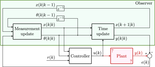
Figure 1: Interpretation of the closed-loop system from the point of view of the nominal model, where the plant is seen as a generator of the “disturbance” $e(k)$ whose effect is rejected by the observer thanks to the disturbance model.

Note that Assumption 6 implicitly requires that model (4) is controllable for all values $\bar{\theta}$ when $\theta(k)\equiv\bar{\theta}$. It also implies that $u(k)\in\mathcal{U}$ by definition, and that the closed-loop system constituted by (4) and (7) is intrinsically robust to vanishing state perturbations affecting both the evolution of the nominal model and the state-feedback signals to the controller. Such a view of the actual control system is depicted in Figure 1, which shows our reinterpretation of the control system as a state-feedback loop with state $(x(k|k-1),\theta(k|k-1))$, output $y(k|k)$ and input $u(k)$ generated by the controller (7) under the feedback perturbations

$$\left[\begin{array}[]{c}\Delta x(k)\\ \Delta\theta(k)\end{array}\right]=\omega(k,e(k)),$$ (9)

caused by the real plant through the measurement-update mapping (6a) of the observer. Clearly, when $e(k)=0$ the measurement update block becomes an all-pass filter having no effect on the control loop, which recovers its nominal behavior given by the evolution of the model equations (4) under the input $u(k)$ generated by (7). In other words, the dynamics of the plant become completely irrelevant in the way the state observer and controller evolve when $e(k)=0$. Indeed, the following theorem shows that if $e(k)$ vanishes asymptotically then the output $y(k)$ of plant (1) perfectly tracks $r(k)$.

Theorem 1.

Consider the closed-loop system constituted by (1) under the control law $u(k)=\kappa(x(k|k),r(k),\theta(k|k))$, where $x(k|k)$ and $\theta(k|k)$ are obtained by (6). Let Assumptions 1–6 hold. Then, for any initial plant state $x_{\mathrm{p}}(0)\in\mathcal{X}_{\mathrm{p}0}$, convergence of the nonlinear observer (6), i.e.,

$$\lim_{k\rightarrow\infty}e(k)=0,$$ (10)

implies asymptotic perfect tracking

$$\lim_{k\rightarrow\infty}y(k)-r(k)=0.$$ (11)

Moreover, $u(k)\in\mathcal{U}$ for all $k\geq 0$ and there exists a time index $k_{f}\geq 0$ such that $y(k)\in\mathcal{Y}$ for all $k\geq k_{f}$.

Proof.

Consider the perturbed dynamical system

$$x(k{+}1|k) =f(x(k|k{-}1){+}\Delta x(k),u(k),d(k|k{-}1){+}\Delta d(k)),$$

$$\theta(k{+}1|k) =\theta(k|k{-}1){+}\Delta\theta(k),$$

$$u(k) =\kappa(x(k|k{-}1){+}\Delta x(k),r(k),\theta(k|k{-}1){+}\Delta\theta(k)),$$

where $\Delta x(k)$, $\Delta\theta(k)$ are given by (9) and

$$\Delta d(k) =h(x(k|k-1)+\Delta x(k),u(k),\theta(k|k-1)+\Delta\theta(k))$$

$$\quad-d(k|k-1).$$

Since, by Assumption 5, the observer feedback $\omega$ is continuous with respect to the output estimation error in a neighborhood of the origin and $\lim_{k\rightarrow\infty}e(k)=0$, then from (6a) we have that the perturbations $\Delta x(k)\rightarrow 0$ and $\Delta\theta(k)\rightarrow 0$ as $k\rightarrow\infty$. By Assumption 3, function $h$ is continuous with respect to $x$ and $d$, so that also $\Delta d(k)\rightarrow 0$. Hence, by Assumptions 4 and 6, we have that $g(x(k|k-1),d(k|k-1))-r(k)\rightarrow 0$ and, finally, since $y(k)-y(k|k-1)=e(k)\rightarrow 0$, also that the actual tracking error

$$y(k)-r(k) =y(k)-y(k|k-1)+y(k|k-1)-r(k)$$

$$=e(k)+g(x(k|k-1),d(k|k-1))-r(k)\rightarrow 0.$$

Since by Assumption 1 $r(k)\in{\rm int}(\mathcal{Y})$ and $y(k)-r(k)\rightarrow 0$, then there exists $k_{f}\in\mathbb{N}$ such that $y(k)\in\mathcal{Y}$ $\forall k\geq k_{f}$. ∎

Note that Assumption 2 has not been explicitly mentioned in the proof of Theorem 1, but in light of the result of the theorem, the condition $x_{\mathrm{p}}(0)\in\mathcal{X}_{\mathrm{p}0}$ is a necessary requirement for (10) and (11) to hold.

We finally remark that the assumption in (10) might be perceived as rather strong. However, note that Assumption 4 guarantees that model (4) can perfectly reproduce the input/output signals from the plant (1) under perfect tracking conditions for a particular value of $\bar{\theta}$ and Assumption 6 guarantees that the controller can make the model track the reference for the same $\bar{\theta}$. Therefore, assumption (10) amounts to having a well-chosen disturbance model and a well-designed state observer. Note that this is a common assumption in the literature on offset-free MPC (see, e.g., [6, Assumption 9]).

III Offset-free EKF-based Nonlinear MPC

The convergence result proved in the previous section is rather general and conceptual. We next show how the result is applied to the frequently used combination of the Extended Kalman Filter (EKF) as state observer and Nonlinear MPC (NMPC) as controller. Additionally, the reference signals $x_{\mathrm{r}}(k+j)$, $u_{\mathrm{r}}(k+j)$ given to the NMPC controller are generated from the future reference preview $r(k+j)$ using the estimated disturbance model parameters $\theta(k|k)$ obtained from the EKF.

We note that the EKF and NMPC presented in the sequel do not immediately guarantee the satisfaction of Assumption 6, in general extra care should be taken to prove that it holds. Such an analysis is beyond the scope of this paper.

III-A Observer: Extended Kalman Filter

When considering the EKF, we take the following particularization of the prediction model (4):

$$x(k+1) =f(x(k),u(k),d_{x}(k)),$$ (12)

$$d_{x}(k) =h_{x}(x(k),u(k),\theta(k)),$$

$$d_{y}(k) =h_{y}(x(k),\theta(k)),$$

$$y(k) =g(x(k),d_{y}(k)),$$

where the disturbance $d$ is split into the process disturbance $d_{x}\in\mathbb{R}^{n_{d_{x}}}$ and the output disturbance $d_{y}\in\mathbb{R}^{n_{d_{y}}}$, and the disturbance function $h$ into $h_{x}\colon\mathbb{R}^{n_{x}}\times\mathbb{R}^{n_{u}}\times\mathbb{R}^{n_{\theta}}\to\mathbb{R}^{n_{d_{x}}}$ and $h_{y}\colon\mathbb{R}^{n_{x}}\times\mathbb{R}^{n_{\theta}}\to\mathbb{R}^{n_{d_{y}}}$. Clearly, model (4) can be recovered from (12) by taking $d=[d_{x}^{\top}~{}d_{y}^{\top}]^{\top}\in\mathbb{R}^{n_{d}}$ and $h$ similarly. We note that $d$ is split so that the measurement-update of the EKF does not depend on the value of $u(k)$, as seen in the sequel.

Model (12) can be interpreted as a combined model in which $f_{n}(x,u)\doteq f(x,u,0)$ and $g_{n}(x)\doteq g(x,0)$ capture a nominal model (either physics-based or black-box) estimated off-line from a set of input/output data $\{u(k),y(k)\}$, and the disturbance model is used for on-line adaptation to match the data measured from the real plant.

In particular, by assuming that function $g$ is differentiable, $f$ is differentiable with respect to $(x,d_{x})$, and $h_{x}$ and $h_{y}$ with respect to $(x,\theta)$, one can estimate $(x(k),\theta(k))$ by the following EKF with measurement updates

$$d_{y}(k|k-1) =h_{y}(x(k|k-1),\theta(k|k-1)),$$ (13a)

$$e(k) =y(k)-g(x(k|k-1),d_{y}(k|k-1)),$$ (13b)

$$B(k) =C(k)P(k|k-1)C^{\prime}(k)+Q_{y}(k),$$ (13c)

$$M(k) =P(k|k-1)C^{\prime}(k)B(k)^{-1},$$ (13d)

$$\begin{bmatrix}x(k|k)\\ \theta(k|k)\end{bmatrix} =\begin{bmatrix}x(k|k-1)\\ \theta(k|k-1)\end{bmatrix}+M(k)e(k),$$ (13e)

$$d_{y}(k|k) =h_{y}(x(k|k),\theta(k|k)),$$ (13f)

$$P(k|k) =\big{(}I-M(k)C(k)\big{)}P(k|k-1),$$ (13g)

and time update

$$d_{x}(k|k) =h_{x}(x(k|k),u(k),\theta(k|k)),$$ (13h)

$$x(k+1|k) =f(x(k|k),u(k),d_{x}(k|k)),$$ (13i)

$$\theta(k+1|k) =\theta(k|k),$$ (13j)

$$P(k+1|k) =A(k)P(k|k)A^{\prime}(k)+Q(k),$$ (13k)

where

$${}\mkern-10.0muC(k) =\begin{bmatrix}\left(\frac{\partial g}{\partial x}+\frac{\partial g}{\partial d_{y}}\frac{\partial h_{y}}{\partial x}\right)&\frac{\partial g}{\partial d_{y}}\frac{\partial h_{y}}{\partial\theta}\end{bmatrix}\vline_{x(k|k-1),\theta(k|k-1)},$$ (13l)

$${}\mkern-10.0muA(k) =\begin{bmatrix}\left(\frac{\partial f}{\partial x}+\frac{\partial f}{\partial d_{x}}\frac{\partial h_{x}}{\partial x}\right)&\frac{\partial f}{\partial d_{x}}\frac{\partial h_{x}}{\partial\theta}\\ 0&I\end{bmatrix}\vline_{x(k|k),\theta(k|k),u(k)},$$ (13m)

$${}\mkern-10.0muQ(k) =\begin{bmatrix}Q_{x}(k)&0\\ 0&Q_{\theta}(k)\end{bmatrix},$$ (13n)

and $Q_{x}(k)$, $Q_{\theta}(k)$, and $Q_{y}(k)$ are positive semidefinite matrices representing, respectively, the covariance matrices of process noise $\xi(k)\in\mathbb{R}^{n_{x}}$, parameter noise $\xi_{\theta}(k)\in\mathbb{R}^{n_{\theta}}$, and output noise $\zeta(k)\in\mathbb{R}^{p}$ according to the following extension of model (4)

$$x(k+1) =f(x(k),u(k),d(k))+\xi_{x}(k),$$ (14)

$$y(k) =g(x(k),d(k))+\zeta(k),$$

$$d(k) =h(x(k),u(k),\theta(k))+\xi_{\theta}(k),$$

that is merely used to design the observer (13).

III-B Controller: Nonlinear MPC

Consider the NMPC formulation

$$\min_{x,u} \sum_{j=0}^{N-1}\ell(x_{j},u_{j},x_{\mathrm{r}}(k{+}j),u_{\mathrm{r}}(k{+}j))+V_{\mathrm{f}}(x_{N},x_{\mathrm{r}}(k{+}N))$$ (15a)

$$\mathrm{s.t.}\ x_{0}=x(k|k),$$ (15b)

$$x_{j+1}=f(x_{j},u_{j},d_{j}),j\in\mathbb{N}_{0}^{N-1},$$ (15c)

$$d_{j}=h(x_{j},u_{j},\theta(k|k)),j\in\mathbb{N}_{0}^{N-1},$$ (15d)

$$y_{j}=g(x_{j},d_{j}),j\in\mathbb{N}_{0}^{N-1},$$ (15e)

$$y_{j}\in\mathcal{Y},\;u_{j}\in\mathcal{U},j\in\mathbb{N}_{0}^{N-1},$$ (15f)

$$x_{N}\in\mathcal{X}_{\mathrm{f}}(x_{\mathrm{r}}(k+N)),$$ (15g)

where $\ell(x_{\mathrm{r}}(k),u_{\mathrm{r}}(k),x_{\mathrm{r}}(k),u_{\mathrm{r}}(k))=0$, for all $k\in\mathbb{N}$, and

$$\ell(x_{j},u_{j},x_{\mathrm{r}}(k+j),u_{\mathrm{r}}(k+j))\geq\alpha_{\ell}\left(\|x_{j}-x_{\mathrm{r}}(k+j)\|\right),$$

for all $u_{j},u_{\mathrm{r}}(k+j)\in\mathcal{U}$ and all $k\in\mathbb{N}$, where $\alpha_{\ell}\colon\mathbb{R}\to\mathbb{R}$ is a class $\mathcal{K}_{\infty}$ function. Moreover, $V_{\mathrm{f}}(x_{\mathrm{r}}(k+N),x_{\mathrm{r}}(k+N))=0$ and $V_{\mathrm{f}}(x_{N},x_{\mathrm{r}}(k+N))\geq\alpha_{V_{\mathrm{f}}}(\|x_{N}-x_{\mathrm{r}}(k+N)\|)$ for all $k\in\mathbb{N}$, where $\alpha_{V_{\mathrm{f}}}\colon\mathbb{R}\to\mathbb{R}$ is a class $\mathcal{K}_{\infty}$ function. Finally, there exists a control law $\kappa_{\mathrm{f}}\colon\mathbb{R}^{n_{x}}\times\mathbb{R}^{n_{x}}\times\mathbb{R}^{n_{\theta}}\to\mathcal{U}$ such that $u_{N}\doteq\kappa_{\mathrm{f}}(x_{N},x_{\mathrm{r}}(k+N),\theta(k|k))$ satisfies

$$f(x_{N},u_{N},d_{N})\in\mathcal{X}_{\mathrm{f}}(x_{\mathrm{r}}(k+N)),$$

$$g(x_{N},d_{N})\in\mathcal{Y},$$

$$V_{\mathrm{f}}(x_{N},x_{\mathrm{r}}(k+N))-V_{\mathrm{f}}(f(x_{N},u_{N},d_{N}),x_{\mathrm{r}}(k+N))$$

$$\hskip 80.00012pt\leq-\ell(x_{N},u_{N},x_{\mathrm{r}}(k+N),u_{\mathrm{r}}(k+N)),$$

for all $x_{N}\in\mathcal{X}_{\mathrm{f}}(x_{\mathrm{r}}(k+N))$, where $d_{N}=h(x_{N},u_{N},\theta(k|k))$. The above NMPC scheme defines a controller by applying the value $u(k)=u_{0}^{*}$, where $u_{0}^{*}$ is the first control move obtained from the optimal solution $(x^{*},u^{*},d^{*},y^{*})$ of (15). The scheme guarantees that the closed-loop system made by the nominal model (4) and the NMPC controller asymptotically tracks the reference signal while satisfying the prescribed constraints for suitable initial states and reference values (see, e.g., [3]).

In order to compute suitable reference signals $x_{\mathrm{r}}(k+j)$, $u_{\mathrm{r}}(k+j)$, $d_{\mathrm{r}}(k+j)$ required in (15), consider the following infinite-horizon reference optimization problem

$$\min\limits_{{\rm\bf{\hat{x}}}_{\mathrm{r}},{\rm\bf{\hat{u}}}_{\mathrm{r}}} \;\sum_{j=0}^{\infty}\ell_{\mathrm{r}}(\hat{x}_{\mathrm{r}}(k+j),\hat{u}_{\mathrm{r}}(k+j))$$ (16)

$$\mathop{\rm s.t.}\nolimits \;r(k+j)=g(\hat{x}_{\mathrm{r}}(k+j),\hat{d}_{\mathrm{r}}(k+j)),$$

$$\;\hat{x}_{\mathrm{r}}(k+j+1)=f(\hat{x}_{\mathrm{r}}(k+j),\hat{u}_{\mathrm{r}}(k+j),\hat{d}_{\mathrm{r}}(k+j)),$$

$$\;\hat{d}_{\mathrm{r}}(k+j)=h(\hat{x}_{\mathrm{r}}(k+j),\hat{u}_{\mathrm{r}}(k+j),\theta(k|k)),$$

where ${\rm\bf{\hat{x}}}_{\mathrm{r}}=\{\hat{x}_{\mathrm{r}}(k+j)\}_{j=0}^{\infty}$ and ${\rm\bf{\hat{u}}}_{\mathrm{r}}=\{\hat{u}_{\mathrm{r}}(k+j)\}_{j=0}^{\infty}$ are, respectively, the state and input reference sequences associated with the reference trajectory $\{r(k+j)\}_{j=0}^{\infty}$, and the cost function $\ell_{\mathrm{r}}\colon\mathbb{R}^{n_{x}}\times\mathbb{R}^{n_{u}}\to\mathbb{R}$ is any convex function that can be used to make the selection unique in case of multiple solutions. At each sample time $k$, the reference signals $x_{\mathrm{r}}(k+j)$ and $u_{\mathrm{r}}(k+j)$ of (15) are taken from the optimal solution of (16).

A special case of (16) is a constant set-point $r(k+j)\equiv r(k)$, $\forall j\in\mathbb{N}$, for which a feasible solution ${\rm\bf{\hat{x}}}_{\mathrm{r}},{\rm\bf{\hat{u}}}_{\mathrm{r}}$ is given by solving the steady-state equations

$$r(k) =g(\hat{x}_{\mathrm{r}}(k),\hat{d}_{\mathrm{r}}(k)),$$ (17)

$$\hat{x}_{\mathrm{r}}(k) =f(\hat{x}_{\mathrm{r}}(k),\hat{u}_{\mathrm{r}}(k),\hat{d}_{\mathrm{r}}(k)),$$

$$\hat{d}_{\mathrm{r}}(k) =h(\hat{x}_{\mathrm{r}}(k),\hat{u}_{\mathrm{r}}(k),\theta(k|k)).$$

In a practical setting, we can modify (16) to only consider $M\in\mathbb{N}$ future samples of the reference signal, i.e., to consider problem (16) for $j\in\mathbb{N}_{0}^{M}$, instead of $j\in\mathbb{N}_{0}^{\infty}$.

Another interesting instance of (16) is the special case of periodic reference signals with period $T$, i.e., reference signals satisfying $r(k+j+T)=r(k+j)$, $\forall j\in\mathbb{N}$. In this case, problem (16) would consider $j\in\mathbb{N}_{0}^{T-1}$, instead of $j\in\mathbb{N}_{0}^{\infty}$, and include the additional constraint $\hat{x}_{\mathrm{r}}(k)=\hat{x}_{\mathrm{r}}(k+T)$.

III-C Comparison with set-point tracking using constant disturbance models

The case of constant disturbance models (see, e.g., [6])

$$x(k+1) =F(x(k),u(k),d(k)),$$ (18)

$$d(k+1) =d(k),$$

$$y(k) =G(x(k),d(k)),$$

is a special case of the general disturbance model (4), obtained by setting ${n_{\theta}}={n_{d}}$, $f(x,u,d)=F(x,u,d)$, $g(x,d)=G(x,d)$, $d_{x}(k)=d_{y}(k)=\theta(k)$ and $h(x,u,\theta)=\theta$. Vice versa, given the model in (4), one can obtain the model in (18) by setting ${n_{d}}={n_{\theta}}$, $d(k)=\theta(k)$, $F(x,u,d)=f(x,u,h(x,u,d))$, and $G(x,d)=g(x,h(x,u,d))$. It is therefore apparent that the two disturbance modeling frameworks are mathematically equivalent. However, we believe that our framework has the advantage of being more structured, as it explicitly models the disturbance vector as the output of a parametric nonlinear model of the state and input vectors, with $\theta$ being the vector of disturbance model parameters, while in (18), the underlying modeling assumption is that the disturbance is an unknown constant, which is fully justified by the fact that the emphasis is on compensating steady-state errors when tracking constant set-points.

We remark also that in [6] the authors assume that the number ${n_{x}}$ of model states is equal to the order ${n_{x_{\mathrm{p}}}}$ of the plant state $x_{\mathrm{p}}$, while in our paper we do not make such an assumption. We do not even assume that ${n_{x_{\mathrm{p}}}}$ is known.

IV Numerical examples

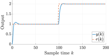
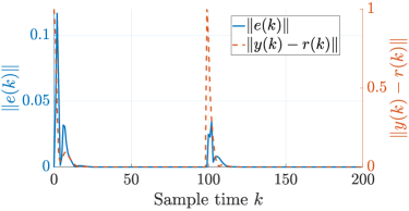
(a) Polynomial disturbance model

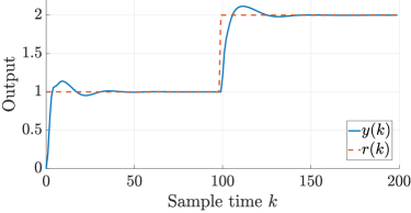
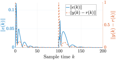
(b) Constant disturbance model

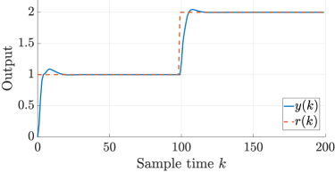
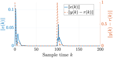
(c) FNN disturbance model

Figure 2: Van der Pol plant. Closed-loop tracking of a piecewise-constant reference using different disturbance models.

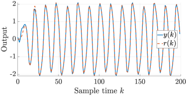
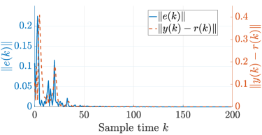
(a) Polynomial disturbance model

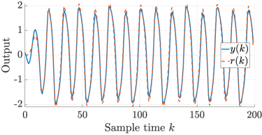
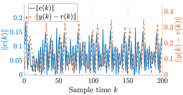
(b) Constant disturbance model

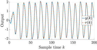
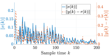
(c) FNN disturbance model

Figure 3: Van der Pol plant. Closed-loop tracking of a generic reference trajectory using different disturbance models.

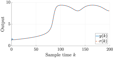
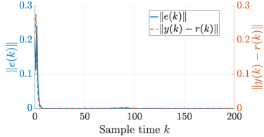
(a) Polynomial disturbance model

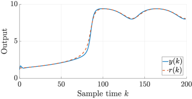
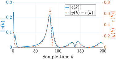
(b) Constant disturbance model

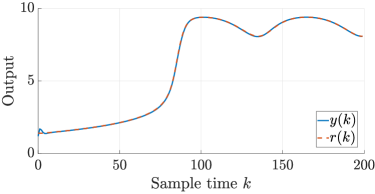
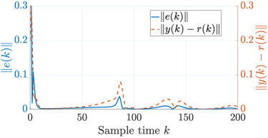
(c) FNN disturbance model

Figure 4: CSTR plant. Closed-loop tracking of a generic reference trajectory using different disturbance models.

This section contains numerical results showing the use of the proposed disturbance model for offset-free tracking of generic references. We start with an academic example, where we show that a proper (but generally impractical) choice of the disturbance model leads to a prediction error $e(k)$ that vanishes to $0$, leading to perfect offset-free tracking. We then show a more realistic case study, where we showcase the good practical performance of the proposed disturbance scheme when compared to the classical constant disturbance model.

All the results shown in this section use the MATLAB interface of CasADi [16, version 3.6.0], selecting IDAS [17] as the numerical integrator and IPOPT [18] as the optimization solver.

IV-A Van der Pol oscillator

We consider the Van der Pol oscillator system, whose dynamics are governed by the second-order differential equation

$$\frac{d^{2}v}{dt^{2}}=\mu(1-\beta v^{2})\frac{dv}{dt}-v-\rho u,$$ (19)

where $v\in\mathbb{R}$ is its position coordinate, $u\in\mathbb{R}$ its control input, and the scalars $\mu,\beta,\rho\geq 0$ are its parameters. We obtain (1) by numerically integrating (19) with a sample time of $0.5$ seconds taking $x_{\mathrm{p}}=(\frac{dv}{dt},v)$, $y=v$, and $\mu=\beta=\rho=1$.

We obtain the prediction model (12) by taking the same model as (1) but considering that we have inaccurately estimated the system parameters; we take $\mu=0.8$, $\beta=0.9$ and $\rho=0.8$. We consider three disturbance models:

1. Constant Disturbance Model (CDM). We take $y=v+d_{y}$, $h_{x}=0$, $h_{y}=\theta$. This is the classical output disturbance model capable of achieving offset-free tracking for piecewise-constant references [6, 8].

2. Polynomial Disturbance Model (PDM). We take $h_{y}=0$, and $h_{x}(x,u,\theta)$ as a polynomial with terms capturing all possible terms of the ordinary differential equation of the plant, i.e., of (19). That is, denoting $\dot{v}\doteq\frac{dv}{dt}$ and the $i$-th element of $\theta\in\mathbb{R}^{10}$ as $\theta_{i}$, we take

   $$h_{x}(x,u,\theta) =\theta_{1}+\theta_{2}\dot{v}+\theta_{3}\dot{v}^{2}+\theta_{4}v+\theta_{5}v^{2}$$

   $$\quad+\theta_{6}\dot{v}v+\theta_{7}\dot{v}^{2}v+\theta_{8}\dot{v}v^{2}+\theta_{9}\dot{v}^{2}v^{2}+\theta_{10}u.$$

   Then, $d_{x}\in\mathbb{R}$ is added to (19) and included in its numerical integration. The idea of this disturbance model is to guarantee the existence of a value of $\theta$ such that the prediction model (12) perfectly captures the real system dynamics (19).

3. Feedforward neural network (FNN). We take $h_{x}$ as a FNN with input $(x,u)\in\mathbb{R}^{{n_{x}}\times{n_{u}}}$, output $d_{x}\in\mathbb{R}^{n_{x}}$, two hidden layers with $6$ neurons each, sigmoid activation function for the hidden layers, and linear activation function for the output layer. We also take $h_{y}$ as a similar FNN, but with input $x\in\mathbb{R}^{n_{x}}$, output $d_{y}\in\mathbb{R}^{p}$ and a single hidden layer with $4$ neurons. The parameters of the two FNNs, i.e., the weights and bias terms of the layers, are stacked in vectors $\theta_{x}$ and $\theta_{y}$, such that $\theta=(\theta_{x},\theta_{y})$. We initialize $\theta_{x}$ and $\theta_{y}$ using the Xavier initialization procedure [19] with zero bias terms. Inspired by [15], this disturbance model is essentially a recurrent neural network (RNN) that is trained online using the EKF to capture the discrepancy between the dynamics of the prediction model and the real system.

We construct the NMPC controller (15) with a prediction horizon $N=5$, taking a terminal equality constraint $x_{N}=x_{\mathrm{r}}(k+N)$ in (15g) and using the classical stage cost function

$$\ell(x,u,x_{r},u_{r}) =\|x-x_{r}\|^{2}_{W_{x}}+\|u-u_{r}\|^{2}_{W_{u}},$$

with $W_{x}=10I_{n_{x}}$ and $W_{u}=I_{n_{u}}$. A terminal cost $V_{\mathrm{f}}$ is not included because it is not needed due to the use of the terminal equality constraint. We don’t consider any constraints on the input nor on the output of the system. At each sample time, the future $N$ samples of the reference trajectories $x_{\mathrm{r}}(k+j)$ and $u_{\mathrm{r}}(k+j)$ for the NMPC controller (15) are computed from (16) taking the stage cost function as

$$\ell_{r}(\hat{x}_{\mathrm{r}}(k+j),\hat{u}_{\mathrm{r}}(k+j))=\|\hat{u}_{\mathrm{r}}(k+j)-u_{\mathrm{r}}(k+j)\|^{2},$$

where $u_{\mathrm{r}}(k)$ is the reference signal given by Assumption 1.

Test	Dist. model	${n_{d_{x}}}$	${n_{d_{y}}}$	${n_{\theta}}$	$Q_{x}$	$Q_{y}$	$Q_{\theta}$
	CDM	0	1	1	$I_{n_{x}}$	$0.25I_{p}$	$I_{n_{\theta}}$
Fig. 2 (Fig. 4)	PDM	1 (2)	0	10 (7)	$I_{n_{x}}$	$0.25I_{p}$	$I_{n_{\theta}}$
	FNN	2	1	97	$I_{n_{x}}$	$0.25I_{p}$	$I_{n_{\theta}}$
	CDM	0	1	1	$I_{n_{x}}$	$0.25I_{p}$	$I_{n_{\theta}}$
Fig. 3	PDM	1	0	10	$10^{-10}I_{n_{x}}$	$0.25I_{p}$	$50I_{n_{\theta}}$
	FNN	2	1	97	$10^{-10}I_{n_{x}}$	$0.25I_{p}$	$50I_{n_{\theta}}$

TABLE I: Dimensions and EKF parameters of each test.

We perform two tests for each of the above disturbance models, one using a piecewise-constant reference and another for a generic reference trajectory. The results are shown, respectively, in Figures 2 and 3. Table I shows the parameters of the EKFs (13) used in each of the tests. Figure 2 shows that all three disturbance models achieve offset-free tracking of piecewise-constant references. This is a well-known result in the case of the CDM [6], which does not hold for non-constant reference trajectories as shown in Figure 3b. On the other hand, Figure 3a shows how the proposed disturbance model is capable of achieving offset-free tracking if Assumptions 1–6 are satisfied, as stated in Theorem 1. Indeed, the parameters $\theta$ of the disturbance model converge to

$$\theta=(0,0.2,0,0,0,0,0,-0.28,0,0.2),$$

which is the value for which the prediction model (4) is equivalent to the real plant (1). We note that in a real setting, a polynomial disturbance model capable of capturing the exact system dynamics will generally not be available. In this case, the use of a more general disturbance model, such as the FNN disturbance model, still provides better reference tracking than a simple CDM, as illustrated in Figure 3c.

IV-B Continuous stirring tank reactor

We now consider the continuous stirring tank reactor (CSTR) system from the MPC toolbox for MATLAB [20]. The two states of the system are the temperature of the reactor $T_{r}$ and the concentration $C_{A}$ of the reactant $A$, the input is the temperature of the coolant $T_{c}$ and the output is $C_{A}$. The control objective is to make $C_{A}$ track a given reference trajectory. We obtain a discrete-time plant model (1) by integrating its ordinary differential equations with a sample time of $0.5$ seconds. As in Section IV-A, we take the prediction model (12) by changing some of the parameters of the plant model (1). We consider the same disturbance models described in Section IV-A, although in this case the PDM is taken as a copy of the plant model (1). We also take the same parameters for the reference generator (16) and NMPC controller (15), with the exception of $W_{x}$, which we take as

$$W_{x}=\begin{bmatrix}1&0\\ 0&0.1\end{bmatrix}.$$

Figure 4 shows the closed-loop results of the CSTR system tracking a generic reference trajectory. The parameters of the EFK are shown in Table I. Figure 4a shows that the use of a simple disturbance model designed to capture the discrepancy between the real plant and the prediction model can lead to near-perfect reference tracking. The CDM provides good results when the reference changes slowly, as seen in the first $50$ sample times of Figure 4b. However, its performance degrades significantly otherwise. Finally, once again, Figure 4c shows how a FNN can provide very good tracking results.

V Conclusions

This paper proposed a specialization of the classical state disturbance model and an extension of the target calculation problem in the presence of future reference previews, motivating its use by presenting two numerical examples where our approach outperforms the classical constant disturbance model. In particular, we showed how an appropriately chosen nonlinear disturbance model can lead to offset-free tracking of generic reference trajectories. Moreover, we showed that the use of a RNN as the nonlinear disturbance model can provide better results than the constant disturbance model, even when the assumptions of the proposed disturbance model are not fully satisfied. Future research will be devoted to extending the theory of offset-free NMPC, for example by removing some strong assumptions such as $e(k)\rightarrow 0$.

References

• [1] K. H. Ang, G. Chong, and Y. Li, “PID control system analysis, design, and technology,” IEEE Transactions on Control Systems Technology, vol. 13, no. 4, pp. 559–576, 2005.
• [2] B. Recht, “A tour of reinforcement learning: The view from continuous control,” Annual Review of Control, Robotics, and Autonomous Systems, vol. 2, pp. 253–279, 2019.
• [3] J. B. Rawlings, D. Q. Mayne, and M. Diehl, Model predictive control: theory, computation, and design, vol. 2. Nob Hill Publishing Madison, WI, 2017.
• [4] F. Borrelli, A. Bemporad, and M. Morari, Predictive Control for Linear and Hybrid Systems. Cambridge University Press, 2017.
• [5] G. Pannocchia, “Offset-free tracking MPC: A tutorial review and comparison of different formulations,” in 2015 European control conference (ECC), pp. 527–532, IEEE, 2015.
• [6] G. Pannocchia, M. Gabiccini, and A. Artoni, “Offset-free MPC explained: novelties, subtleties, and applications,” IFAC-PapersOnLine, vol. 48, no. 23, pp. 342–351, 2015.
• [7] G. Pannocchia and A. Bemporad, “Combined design of disturbance model and observer for offset-free model predictive control,” IEEE Transactions on Automatic Control, vol. 52, no. 6, pp. 1048–1053, 2007.
• [8] M. Morari and U. Maeder, “Nonlinear offset-free model predictive control,” Automatica, vol. 48, no. 9, pp. 2059–2067, 2012.
• [9] G. Betti, M. Farina, and R. Scattolini, “A robust MPC algorithm for offset-free tracking of constant reference signals,” IEEE Transactions on Automatic Control, vol. 58, no. 9, pp. 2394–2400, 2013.
• [10] V. Mirasierra, J. D. Vergara-Dietrich, and D. Limon, “Real-time optimization of periodic systems: A modifier-adaptation approach,” IFAC-PapersOnLine, vol. 53, no. 2, pp. 1690–1695, 2020.
• [11] F. Bonassi, C. Fabio, O. da Silva, and R. Scattolini, “Nonlinear MPC for offset-free tracking of systems learned by GRU neural networks,” IFAC-PapersOnLine, vol. 54, no. 14, pp. 54–59, 2021.
• [12] F. Bonassi, J. Xie, M. Farina, and R. Scattolini, “An offset-free nonlinear MPC scheme for systems learned by neural NARX models,” in 2022 IEEE 61st Conference on Decision and Control (CDC), pp. 2123–2128, IEEE, 2022.
• [13] S. H. Son, J. W. Kim, T. H. Oh, D. H. Jeong, and J. M. Lee, “Learning of model-plant mismatch map via neural network modeling and its application to offset-free model predictive control,” Journal of Process Control, vol. 115, pp. 112–122, 2022.
• [14] A. Caspari, H. Djelassi, A. Mhamdi, L. T. Biegler, and A. Mitsos, “Semi-infinite programming yields optimal disturbance model for offset-free nonlinear model predictive control,” Journal of Process Control, vol. 101, pp. 35–51, 2021.
• [15] A. Bemporad, “Recurrent neural network training with convex loss and regularization functions by extended Kalman filtering,” IEEE Transactions on Automatic Control, vol. 68, no. 9, pp. 5661–5668, 2023.
• [16] J. A. E. Andersson, J. Gillis, G. Horn, J. B. Rawlings, and M. Diehl, “CasADi – A software framework for nonlinear optimization and optimal control,” Mathematical Programming Computation, 2018.
• [17] R. Serban, C. Petra, A. C. Hindmarsh, C. J. Balos, D. J. Gardner, D. R. Reynolds, and C. S. Woodward, “User documentation for IDAS.” \urlhttps://sundials.readthedocs.io/en/latest/idas, 2023.
• [18] A. Wächter and L. T. Biegler, “On the implementation of an interior-point filter line-search algorithm for large-scale nonlinear programming,” Mathematical programming, vol. 106, pp. 25–57, 2006.
• [19] X. Glorot and Y. Bengio, “Understanding the difficulty of training deep feedforward neural networks,” in Proceedings of the thirteenth international conference on artificial intelligence and statistics, pp. 249–256, JMLR Workshop and Conference Proceedings, 2010.
• [20] A. Bemporad, M. Morari, and N. L. Ricker, “Model Predictive Control Toolbox for MATLAB.” \urlhttp://www.mathworks.com/access/helpdesk/help/toolbox/mpc/, 2020. The Mathworks, Inc.