Data-driven Estimation of Under Frequency Load Shedding after Outages in Small Power Systems

Abstract

This paper presents a data-driven methodology for estimating Under Frequency Load Shedding (UFLS) in small power systems. UFLS plays a vital role in maintaining system stability by shedding load when the frequency drops below a specified threshold following loss of generation. Using a dynamic System Frequency Response (SFR) model we generate different values of UFLS (i.e., labels) predicated on a set of carefully selected operating conditions (i.e., features). Machine Learning (ML) algorithms are then applied to learn the relationship between chosen features and the UFLS labels. A novel regression tree and the Tobit model are suggested for this purpose and we show how the resulting non-linear model can be directly incorporated into a Mixed Integer Linear Programming (MILP) problem. The trained model can be used to estimate UFLS in security-constrained operational planning problems, improving frequency response, optimizing reserve allocation, and reducing costs. The methodology is applied to the La Palma island power system, demonstrating its accuracy and effectiveness. The results confirm that the amount of UFLS can be estimated with the Mean Absolute Error (MAE) as small as 0.213 MW for the whole process, with a model that is representable as a MILP for use in scheduling problems such as unit commitment among others.

This study is funded by 2022 National Research Program ‘PROYECTOS DE GENERACIÓN DE CONOCIMIENTO’, Ministerio de Ciencia e Innovación – Agencia Estatal de Investigación, Project PID2022-141765OB-I00

I Introduction

Synchronous generators are being displaced with cleaner, albeit non-synchronously coupled alternatives (like wind and solar), which inadvertently has led to a reduction of inertia, hence incorporating frequency dynamics into the operational planning of power systems is more important than ever. Island power systems are already suffering from a lack of inertia because of their small size. There has been extensive research on how to include frequency dynamics in scheduling optimization problems. Both analytical methods (directly from the swing equation) and data-driven methods (based on dynamic simulations) have been proposed to obtain frequency constraints for inclusion in the operational planning process. Typical frequency response metrics after outages are the Rate of Change of Frequency (RoCoF), quasi-steady-state frequency, and frequency nadir. However, calculating the frequency nadir is much more complicated than the other metrics. To derive the frequency nadir from the swing equation, some simplifying assumptions are needed, and still, the obtained equation is non-linear and non-convex, which makes it challenging to be used in MILP problem formulations. A common assumption in analytical frequency-constrained methods like [1, 2, 3, 4, 5], and many other similar works, is that the provision of reserve increases linearly in time, and all units will deliver their available reserve within a given fixed time. Consequently, the ensuing complicated analytical methods are not necessarily accurate. On the other hand, more recently, ML-based methods have been proposed to incorporate frequency dynamics. For instance, optimal classifier tree is used in [6], deep neural network is used in [7], and logistic regression is used in [8], among other approaches. An analytical frequency constrained Unit Commitment (UC) is compared with data-driven models with the help of ML in [9] and their pros and cons are highlighted.

In smaller systems like islands the frequency can easily exceed the safe threshold after any contingency because usually online units are providing a considerable percentage of the whole demand. In order to maintain the frequency stability of an electrical power system, UFLS schemes are implemented to shed or disconnect a certain amount of load in predefined steps when the frequency drops below a specified threshold following disturbance events. This corrective protection measure helps to balance the power supply and demand and prevents a complete system blackout. Different methods have been introduced to tune and optimize the UFLS scheme for electrical power systems, which can be categorized into conventional and adaptive methods. Conventional UFLS schemes use fixed load shedding steps [10, 11, 12, 13], while adaptive UFLS schemes dynamically adjust the load shedding amount based on real-time system conditions [14, 15, 16, 17]. Although adaptive schemes provide a more optimized and flexible response, as they require more advanced monitoring systems and computational capabilities for real-time monitoring and optimization, they are still not used widely in practice. The performance of both conventional and adaptive methods can be improved by incorporating ML [18, 19].

Depending on the size of the system, it is possible to prevent UFLS activation. Many studies like [7, 20, 21, 22], and others set the frequency dynamic thresholds high enough, so no outage leads to UFLS. This is not possible in a small system, where every online unit is providing a substantial percentage of the demand and any outage can be big enough to trigger the UFLS activation [8]. In such systems co-optimizing UFLS activation and scheduling of the units can have some benefits like:

• Having an estimate of UFLS in the scheduling optimization problem will prevent incidents with poor frequency responses.

• The estimated amount of UFLS can be deduced from the required reserve. There is no need to schedule reserve as much as the biggest outage if eventually the UFLS will be activated after the outage.

• UFLS can be monetized easily and added directly to the objective function of the optimization problem, in order to reduce the overall operation costs.

This paper tries to estimate the amount of UFLS, regardless of the UFLS scheme that is used for the system, through a learning process. The estimation of the amount of UFLS of conventional schemes is however very complicated because of its discrete nature and disturbance-dependent behavior. Given the widespread use of conventional schemes in real systems, it’s the principal focus of this paper. The purpose is to use the estimation of UFLS in the operational planning of small power systems (such as generation UC, Economic Dispatch (ED), reserve allocation, ancillary service scheduling, Renewable Energy Sources (RES) integration, and so on). The operational planning process is usually modeled and solved as an MILP problem. Therefore, it is convenient to limit the hypothesis space of the UFLS estimation models to models that are representable by MILP. Including UFLS estimation in the problem is in a sense equivalent to including frequency dynamics in the operational planning, because poor frequency response subsequently triggers the activation of UFLS.

In order to estimate the amount of UFLS, a dataset generation process is proposed to acquire a set of operating points (potential hourly generation schedules) that can properly describe the system under study. Every possible outage in each set of generation schedules is labeled with its corresponding UFLS. The obtained dataset is carefully analyzed to choose the representative features and then a learning process is proposed. A regression tree model with a novel partitioning algorithm is suggested in this paper. As the UFLS is activated in steps and sheds load in a discrete manner, a regression tree seems most suitable. Our partitioning algorithm exploits the data structure to most effectively represent the regression tree as a MILP [23]. Also, the use of the Tobit model to estimate UFLS is proposed and studied. Although the Tobit model is typically used to describe censored data [24], we found it to be effective to also describe the UFLS, which has a cluster around zero followed by a linearly increasing trend as a function of the features, very similar to zero censored datasets. Additionally, the Tobit model has a simple analytic structure that makes it easy to incorporate into a MILP. Both the suggested regression tree and the Tobit model, alongside their MILP representation are demonstrated in the following. To the best of the author’s knowledge, there’s no prior careful analysis on UFLS estimation or an MILP representation of UFLS in the literature. The rest of the paper is organized as follows; in section II the methodology of the paper is introduced, including the data generation (in section II-A), labeling the data (in section II-B), and the learning process (in section II-C). Then in section III the results for the island under study (La Palma) are presented, including the data generation and analysis (in section III-A), the applied learning process, and its accuracy (in section III-B). Finally, conclusions are drawn in section IV.

II Methodology

II-A Data Generation

In order to estimate the UFLS, a proper set of simulation data is necessary. The training dataset comprises features $x\in\mathcal{X}$ and labels $y\in\mathcal{Y}$. In the case of implementing the estimation of UFLS in the operational planning problems (like UC), features are any measurable quantities from the power system that might help predict the UFLS. These features are extracted from generation combinations, while the labels are obtained from dynamic simulations of UFLS after outages. It is beneficial to use only the features with the most relevant information to predict the label $y$ [25]. In this paper, $y$ is the amount of UFLS following each outage, and variables that are most correlated with the label are chosen as features. As shown later in section III, the selected features for predicting UFLS are available inertia ($\mathcal{H}_{g}$), the weighted gain of turbine-governor model ($\mathcal{K}_{g}$), the amount of lost power ($P_{g}$), and the amount of available reserve ($\mathcal{R}_{g}$), after the outage of generator $g$. The synthetic data generation method introduced in [9], is used here. The obtained dataset consists of all feasible and economical generation combinations in La Palma Island, which is the case study of this paper.

II-B Labeling the Data

The measurements for labeling the data can be obtained by solving high-order differential swing equations, from historical data, or by using SFR models. In this paper, a SFR model is used to analyze the frequency stability of small isolated power systems, such as the La Palma Island, which is the system being studied. The SFR model can reflect the short-term frequency response of such systems. The complete model is explained in [26].

II-C Learning Process

II-C1 Proposed Regression Tree

A regression tree is suggested in this paper to estimate the amount of UFLS since conventional schemes shed load in a discrete manner. Typical regression trees split the feature space into rectangular cells and use a constant value within each cell for prediction. However, if we want to incorporate the model into a MILP, we prefer to have as few cells as possible. Therefore, a novel regression tree is proposed here, which is inspired by [27] but deviates from it in several ways:

• The data shows that using convex regions leads to a far more efficient representation. Therefore, we use linear functions to partition cells, rather than single features.

• Within each cell, a linear model is used instead of a constant, as this further reduces the number of cells.

• For prediction, it’s important to estimate incidents with no UFLS as exactly zero and not a small number. The suggested tree structure is able to achieve that.

Representing such regression tree as MILP is presented later. MILP-representability of many ML methods is exploited in [23].

The suggested regression tree is shown in fig. 1. In this figure, N₀ is the root node. N₁ and N₂ are the nodes of the first layer. A linear function of the features (for example $f_{0}(x)$ for the root node) will split the nodes into two to classify the incidents with a threshold on the labels. Then on the last layer, there are the leaves L₁ to L_L. Linear regression is applied to the samples within each of these leaves.

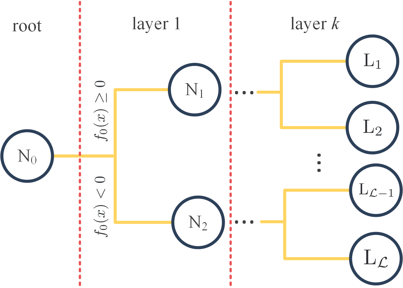
Figure 1: Proposed regression tree.

As the labels of the dataset are already accessible after the labeling process (section II-B) different methods can be applied to split each node. Each splitting function is found by solving a univariate optimization problem, as explained next.

Finding the optimal linear function $f(x)=\beta_{0}+\sum_{i=1}^{p}\beta_{i}x_{i}$, where $p$ is the number of features, to split each cell requires solving a $p+1$ dimensional optimization problem, which finds the coefficients $\beta$ that minimizes the error of the local linear fits in each cell. This is a difficult optimization problem, and also a reason why typical regression trees split only on single features, i.e. only on functions of the form $f(x)=x_{i}-c$ for a single feature $x_{i}$. To reduce the problem of finding $\beta$ to a univariate optimization problem, we propose to employ logistic regression, as follows.

We first introduce a univariate threshold variable $c$ (over which we will optimize), and binary variable $z$, with $z=0$ if $y<c$ (here, $y$ is the amount of UFLS, i.e. the value we try to predict) and $z=1$ otherwise. Define the logistic function as follows:

$$p_{\beta}(x)\coloneqq\frac{1}{1+\exp(-\beta_{0}-\sum_{i=1}^{p}\beta_{i}x_{i})}$$ (1)

The key idea now is that a good split for predicting $y$ should be able to predict $z$ from $x$. Therefore, we find $\beta_{0}$, …, $\beta_{p}$ to maximize the log-likelihood,

$$\sum_{j\in N}z^{(j)}\log p_{\beta}(x^{(j)})+(1-z^{(j)})\log(1-p_{\beta}(x^{(j)}))$$ (2)

where $N$ is the node (as a subset of sample indices) that we are currently trying to split. For any given threshold $c$, denote the maximum likelihood estimate of $\beta$ by $\hat{\beta}(c)$. Consequently, for each $c$, we can split node $N$ into two sub-nodes $N^{\prime}(c)$ and $N^{\prime\prime}(c)$. Now by performing a one-dimensional grid search, we choose $c$ that minimizes the overall error of the local linear models. The splitting can be continued until the tree is able to predict the amount of UFLS with an acceptable accuracy. Note that a simpler tree structure is preferred for two reasons. Firstly, although the accuracy of the model for the dataset in hand might improve by adding more layers, the model will be more susceptible to over-fitting. Secondly, the MILP representation becomes computationally burdensome for more complicated tree structures.

To predict values of the UFLS on each leaf, standard linear regression is used. The maximum likelihood estimate of the parameters of the linear model of leaf L_ℓ can be calculated by finding $\alpha_{0},\dots,\alpha_{p}$ that minimize

$$\sum_{\begin{subarray}{c}j\in\text{L}_{\ell}\end{subarray}}\left(\alpha_{0}+\sum_{i=1}^{p}\alpha_{i}x_{i}^{(j)}-y^{(j)}\right)^{2}$$ (3)

Note that, for this fit, only the samples that are assigned to the leaf L_ℓ of the UFLS data are included, resulting in the summation over indices $j\in\text{L}_{\ell}$.

Putting it all together, we predict $\hat{y}$ from $x$ using the following piecewise linear function

$$\hat{y}(x)=\begin{cases}\alpha_{0}^{1}+\sum_{i=1}^{p}\alpha_{i}^{1}x_{i}&\text{if }x\in\text{L}_{1}\\ \vdots\\ \alpha_{0}^{\ell}+\sum_{i=1}^{p}\alpha_{i}^{\ell}x_{i}&\text{if }x\in\text{L}_{\ell}\\ \vdots\\ \alpha_{0}^{\mathcal{L}}+\sum_{i=1}^{p}\alpha_{i}^{\mathcal{L}}x_{i}&\text{if }x\in\text{L}_{\mathcal{L}}\end{cases}$$ (4)

Encoding the proposed regression tree as MILP: To encode the regression tree (i.e. eq. 4) as an MILP model, first a binary variable $u_{\ell}$ for each leaf L_ℓ needs to be defined, which is equal to 1 if $x$ belongs to leaf L_ℓ. Since $x$ can only belong to one leaf (see (4)), the sum of the binary variables $u$ is equal to 1:

$$\sum_{\ell\in\mathcal{L}}u_{\ell}=1$$ (5)

Further, the binary variables $u$ should be equal to 0 if any of the parent nodes fails. Finally, the decisions at the non-leaf nodes (N₀ to N_N) directly influence the values of the binary variables of the downstream leaves [27]. For instance, if the decision at N₀ is $f_{0}(x)=\hat{\beta}_{0}^{0}+\sum_{i=1}^{p}\hat{\beta}_{i}^{0}x_{i}<0$), then $u_{\ell}=0$ for leaves in the upper subtree, and $u_{\ell}=1$ for leaves in the lower subtree. The following two constraints force $u_{\ell}$ to take these values as a function of $x$:

$$\hat{\beta}_{0}^{0}+\sum_{i=1}^{p}\hat{\beta}_{i}^{0}x_{i}+\underline{\mathcal{M}}_{0}\sum_{\ell\in\mathcal{L}^{\prime}}u_{\ell} \geq\underline{\mathcal{M}}_{0}$$ (6a)

$$\hat{\beta}_{0}^{0}+\sum_{i=1}^{p}\hat{\beta}_{i}^{0}x_{i}+\overline{\mathcal{M}}_{0}\sum_{\ell\in\mathcal{L}^{\prime\prime}}u_{\ell} <\overline{\mathcal{M}}_{0}$$ (6b)

where $\hat{\beta}^{(0)}$ are the obtained logistic regression coefficients for node N₀. $\underline{\mathcal{M}_{0}}$ and $\overline{\mathcal{M}_{0}}$ are lower and upper bounds for the values that $\hat{\beta}_{0}^{0}+\sum_{i=1}^{p}\hat{\beta}_{i}^{0}x_{i}$ can take for any $x$ in N₀. $\mathcal{L}^{\prime}$ and $\mathcal{L}^{\prime\prime}$ are the list of leaves in the upper and lower subtrees of the node N₀. A similar set of constraints must be defined for each node. Now that a binary variable pointing to the correct leaf is accessible, $\hat{y}$ in eq. 4 can be calculated as:

$$\hat{y}=\sum_{\ell\in\mathcal{L}}u_{\ell}\times\left(\alpha_{0}^{\ell}+\sum_{i=1}^{p}\alpha_{i}^{\ell}x_{i}\right)$$ (7)

Equation 7 is non-linear due to the product of binary and continuous variables. To linearize (7), the following sets of constraints need to be defined for each leaf $\ell$,

$$\alpha_{0}^{\ell}+\sum_{i=1}^{p}\alpha_{i}^{\ell}x_{i}-\overline{\mathcal{M}}_{\ell}(1-u_{\ell}) \leq r_{\ell}$$ (8a)

$$\alpha_{0}^{\ell}+\sum_{i=1}^{p}\alpha_{i}^{\ell}x_{i}-\underline{\mathcal{M}}_{\ell}(1-u_{\ell}) \geq r_{\ell}$$ (8b)

$$\overline{\mathcal{M}}_{\ell}u_{\ell} \geq r_{\ell}$$ (8c)

$$\underline{\mathcal{M}}_{\ell}u_{\ell} \leq r_{\ell}$$ (8d)

where $\overline{\mathcal{M}}_{\ell}$ and $\underline{\mathcal{M}}_{\ell}$ are upper and lower bounds of the term $\alpha_{0}^{\ell}+\sum_{i=1}^{p}\alpha_{i}^{\ell}x_{i}$ for all $x\in\text{L}_{\ell}$, and $r_{\ell}$ is an auxiliary variable. Now the linear equation for $\hat{y}$ can be simply written as,

$$\hat{y}=\sum_{\ell\in\mathcal{L}}r_{\ell}$$ (9)

Considering the proposed MILP encoding method, after training the regression tree with $\mathcal{N}$ nodes and $\mathcal{L}$ leaves with the proposed method, to estimate a new observation in a MILP model, $2\times\mathcal{N}$ constraints are needed to present the tree structure, one constraint to one-hot encode the binary variables $u$, $4\times\mathcal{L}+1$ constraints to calculate the linearized $\hat{y}$. Also for each observation, $\mathcal{L}$ new continuous variables and $\mathcal{L}$ binary variables are defined.

II-C2 Tobit Model

Instead of making use of a binary tree and linear regression, we can also consider the standard Tobit model [24]. The model considers $y^{*}=\alpha_{0}+\sum_{i=1}^{p}\alpha_{i}x_{i}+\epsilon$, with $\epsilon\sim N(0,\sigma^{2})$, but instead of $y^{*}$ the following is observed,

$$\hat{y}=\begin{cases}y^{*}&\text{if $y^{*}>0$}\\ 0&\text{otherwise}\end{cases}$$ (10)

The MILP representation is straightforward. Same as before, one binary variable is defined for each side.

$$\alpha_{0}+\sum_{i=1}^{p}\alpha_{i}x_{i}+\underline{\mathcal{M}}u_{R} \geq\underline{\mathcal{M}}$$ (11a)

$$\alpha_{0}+\sum_{i=1}^{p}\alpha_{i}x_{i}+\overline{\mathcal{M}}u_{L} <\overline{\mathcal{M}}$$ (11b)

$$u_{R}+u_{L} =1$$ (11c)

$$\hat{y}=(\alpha_{0}+\sum_{i=1}^{p}\alpha_{i}x_{i})\times u_{R} +0\times u_{L}$$ (11d)

As seen in eq. 11d a variable in binary multiplication appears, which can be linearized as stated before. After training the dataset with the Tobit model, to calculate $\hat{y}$ for each observation in the MILP model, 12 constraints, 2 binary variables, and 2 continuous variables are added.

III Results

The process of data generation, labeling, data analysis, learning model, and the obtained accuracy for the process are presented in this section. The case study is La Palma Island. The data regarding the island is presented in [8].

III-A Data Generation and Analysis

The algorithm presented in [9] is utilized to construct a training dataset for La Palma Island. The power levels are defined using increments of 0.5 MW to form a vector, and all possible combinations of the generators are listed. However, any combinations exceeding the annual thermal generation peak or falling below the annual thermal generation minimum are excluded. The historical thermal generation data for La Palma island indicates that the thermal generation ranges between 36 MW and 16 MW throughout the year. Therefore, the training dataset should only include generation combinations between the maximum and minimum thermal generation limits. Generation combinations that violate the technical requirements are not feasible and are excluded.

The remaining operation points are then sorted by the total value of their quadratic generation cost functions, and the cheaper ones are retained for every thermal generation level. The reason is that these operation points are more likely to appear in the optimized solution. As previously explained, all data points must be labeled with the SFR model. The SFR model is used to calculate the amount of UFLS for each respective outage, with over 110,000 possible outages for the training dataset. The aim is to label all outages with their expected amount of UFLS.

First, let’s look at the correlations between the features and the labels. In fig. 2 the Pearson correlation between available inertia, weighted $K$, lost power, power reserve, and the amount of UFLS is shown on a heatmap.

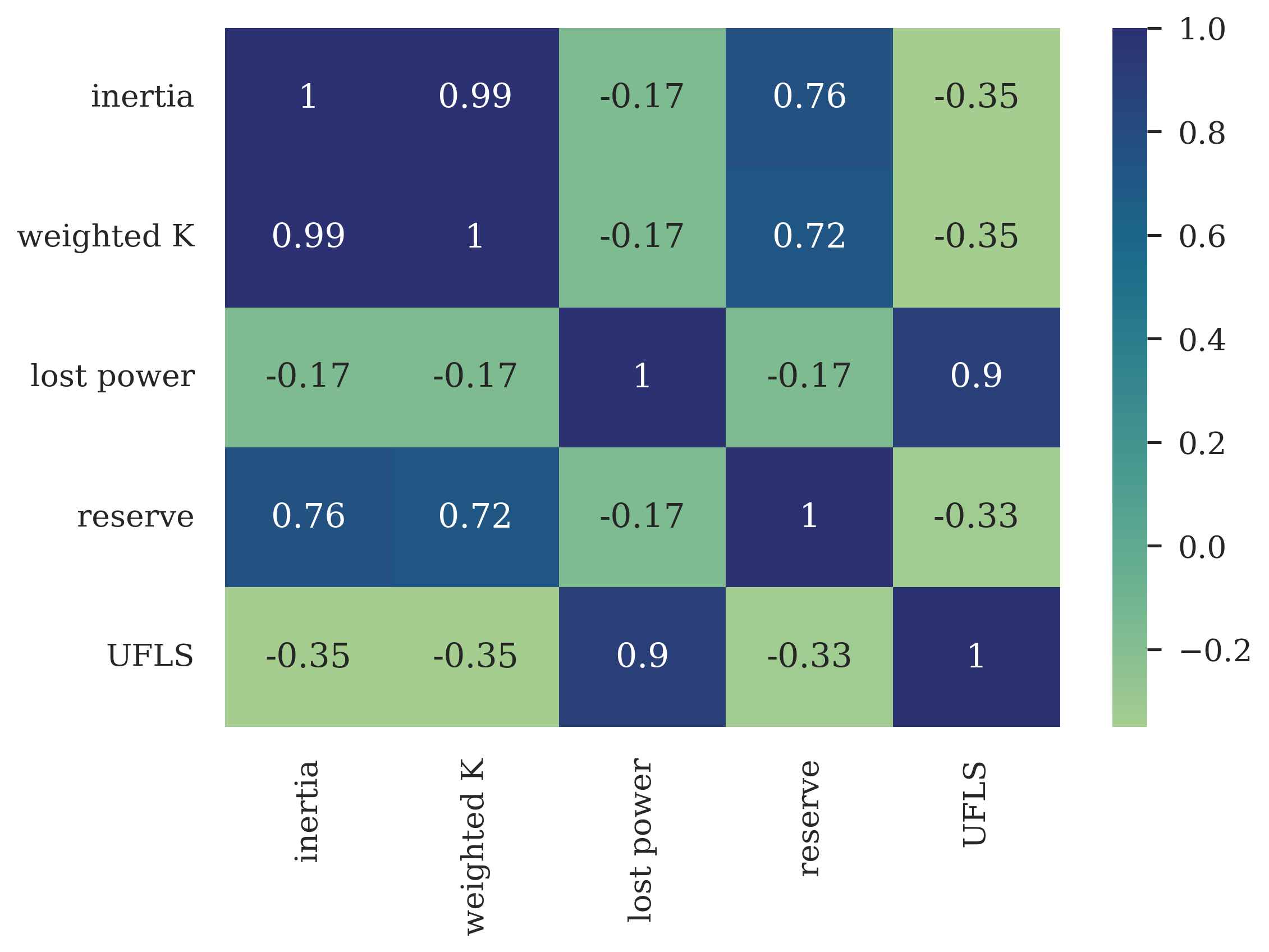
Figure 2: Pearson correlation between inertia, weighted $K$, lost power, power reserve, and the amount of UFLS.

In fig. 3 the Kernel Density Estimate (KDE) plot of inertia, weighted $K$, lost power, power reserve, and the amount of UFLS is depicted in the lower part of the figure. In the upper part of the figure, the scatter plot of the same quantities is depicted. The outages that don’t lead to any UFLS are shown in blue, and outages with positive UFLS are shown in red.

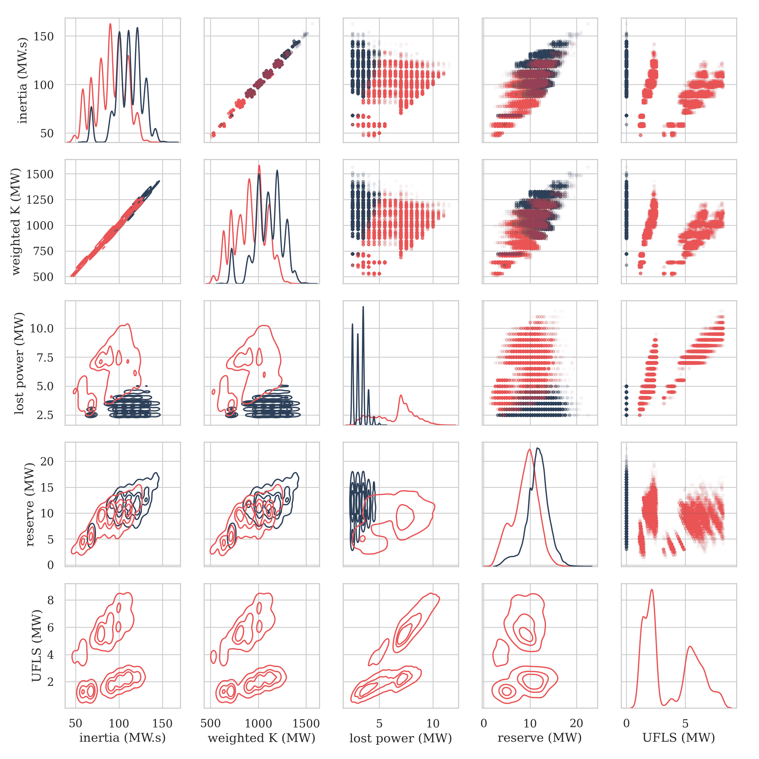
Figure 3: KDE and scatter plot of the features and the labels.

Figure 3 gives a good insight into the distribution of the data and how smooth the data is. This figure clearly shows the complexity of the problem at hand. As the final purpose is to use the estimation of UFLS in the operational planning process, it’s important to estimate the blue incidents in fig. 3 as exactly zero, and not a small number. Although the general relation between the features shown in fig. 3 and the amount of UFLS is complex and non-linear, some trades can be spotted. It seems that the incidents with no UFLS (in blue), and the incidents with some UFLS (in red) cannot be easily distinguished with only one feature. The combination of all features will distinguish blue and red dots with better accuracy. That’s another reason to use methods like logistic regression for splitting the nodes, rather than decision trees that rely on one feature to apply the splits. Both of the methods that were introduced in the methodology (Tobit model and proposed regression tree) are applied to the dataset in order to estimate UFLS.

III-B Learning Process

To train and evaluate the models, the dataset from section III-A is divided randomly into a training dataset (80% of the data) and a test dataset (20% of the data). The learning process is done using the training dataset, and the evaluation is done using the test dataset.

III-B1 With Regression Tree

A grid search is performed to find the optimum tree structure. Different UFLS thresholds for splitting are tried in a loop, starting from zero and with 0.1 MW steps, and the one that leads to overall minimum MAE is chosen. Looking at the distribution of the amount of UFLS in fig. 3 three groups of data can be distinguished: incidents with zero UFLS, incidents with small UFLS (between 0 to 4 MW), and incidents with big UFLS (between 4 to 8 MW). Considering this observation and after performing a grid search to find $c$, the tree structure shown in fig. 4 achieves small MAE while being simple.

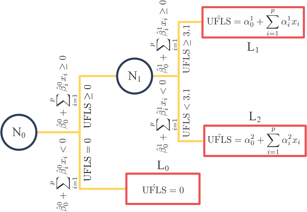
Figure 4: Proposed regression tree with minimum overall MAE.

On the node N₀ the data is classified into positive UFLS and zero UFLS. The split containing zeros doesn’t need any further classification as all of them are equal to zero. On the node N₁ the remaining points are classified into UFLS bigger than 3.1 MW and smaller than 3.1 MW. The estimated amount of UFLS is presented by its corresponding linear regression on each leaf. The obtained data of this tree structure is presented in table I. The scores that are shown in this table are the result of applying the model trained by the training dataset, on the test dataset.

TABLE I: The data of the trained tree.

	intercept	$\times\mathcal{H}_{g}$	$\times\mathcal{K}_{g}$	$\times P_{g}$	$\times\mathcal{R}_{g}$	score
N0	$\beta_{0}^{0}$=1	$\beta_{1}^{0}$=0.516	$\beta_{2}^{0}$=-0.158	$\beta_{3}^{0}$=28.957	$\beta_{4}^{0}$=-1.176	acc=98.8%
N1	$\beta_{0}^{1}$=1	$\beta_{1}^{1}$=-0.003	$\beta_{2}^{1}$=0.004	$\beta_{3}^{1}$=-0.726	$\beta_{4}^{1}$=0.048	acc=94.7%
L0	$\alpha_{0}^{0}$=0	$\alpha_{1}^{0}$=0	$\alpha_{2}^{0}$=0	$\alpha_{3}^{0}$=0	$\alpha_{4}^{0}$=0	MAE =0
L1	$\alpha_{0}^{1}$=-0.104	$\alpha_{1}^{1}$=0.019	$\alpha_{2}^{1}$=0.0001	$\alpha_{3}^{1}$=0.106	$\alpha_{4}^{1}$=-0.057	MAE =0.037 MW
L2	$\alpha_{0}^{2}$=0.006	$\alpha_{1}^{2}$=0.026	$\alpha_{2}^{2}$=-0.002	$\alpha_{3}^{2}$=0.870	$\alpha_{4}^{2}$=-0.176	MAE =0.272 MW

The final MAE of this process will be partly due to the classification errors on the nodes and the regression error on the leaves. In fig. 5 the classification error on different leaves is presented.

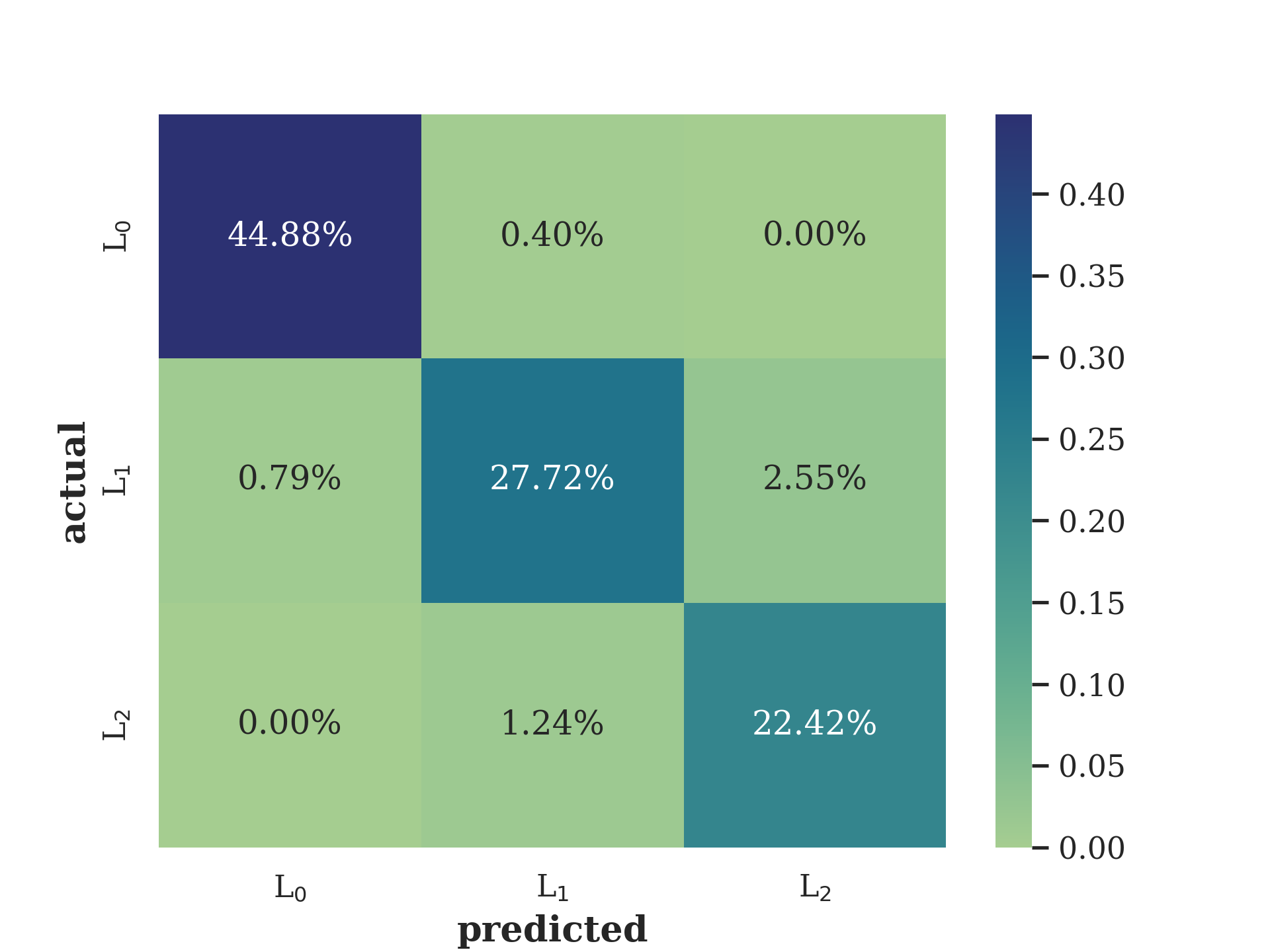
Figure 5: The classification confusion matrix for each class.

The diagonal squares show the percentage of true positive classifications for each class. For example, $95.02\%$ of the whole data has been classified correctly (sum of the diagonal squares). $0.79\%$ of the samples on L₁ are incorrectly classified as L₀. $0.40\%$ of L₀ samples are incorrectly classified as L₁, and so on.

The UFLS for all the samples that are assigned to L₀ is estimated as zero and for L₁ and L₂ linear regression is applied. The residuals (predicted value minus observed labels) of the estimation on the test dataset are shown in fig. 6.

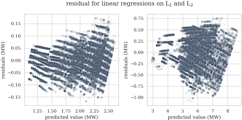
Figure 6: The residual for the regression applied on L₁ and L₂.

Considering the complexity of the problem at hand, and being limited to using linear models, the accuracy is acceptable. The prediction error for the samples in L₁ is always less than 0.15 MW and for L₂ is always less than 1 MW. Note that the samples on L₂ are bigger than the samples on L₁.

Now considering all of the classifications and regression applied in the suggested tree structure, it’s possible to look at the residuals for the whole process, shown in fig. 7.

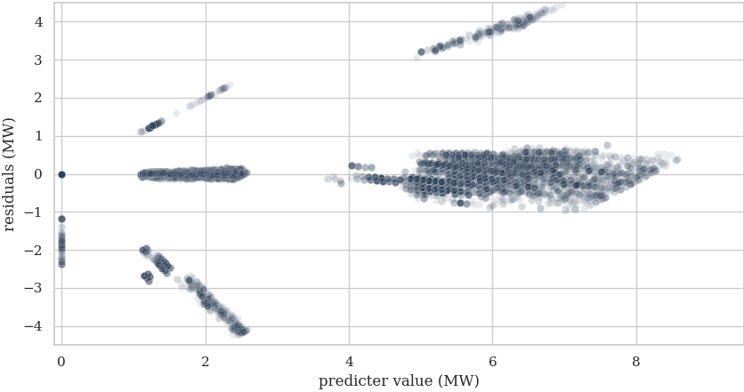
Figure 7: The residual for the suggested regression tree.

Other than regression errors, errors due to misclassification are evident. The bigger residuals are because of the misclassification. That’s why more complicated tree structures wouldn’t improve the overall accuracy in this case. The MAE of the whole process on the test dataset is 0.213 MW. The trained tree can be represented as MILP with the addition of 18 new constraints, 3 continuous variables, and 3 binary variables for every observation.

III-B2 With Tobit Model

The training dataset is trained with the Tobit model (section II-C2). Then it’s applied to the test dataset. The residuals are shown in fig. 8.

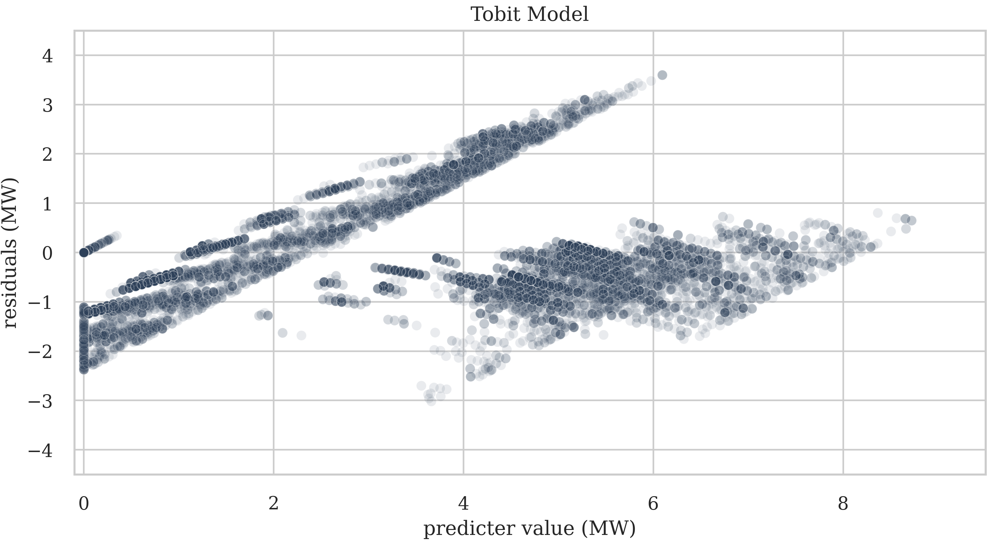
Figure 8: Residuals of the test dataset. The training dataset is trained with Tobit model.

The model has successfully distinguished most of the zero UFLS incidents and pushed them to the negative side so they will be equal to zero in the model. As the model tries to fit all of the positive UFLS incidents with one line, the error is high for some incidents. The overall MAE of the model on the test dataset is 0.4967 MW. The advantage of this model is being easy to implement as MILP. Here is the trained Tobit model,

$$\hat{\text{UFLS}}=\begin{cases}-0.702-0.027\mathcal{H}_{g}-0.001\mathcal{K}_{g}\\ +1.382P_{g}-0.132\mathcal{R}_{g}&\text{if it's}>0\\ 0&\text{otherwise}\end{cases}$$ (12)

According to the eq. 11 the term in eq. 12 can be represented as MILP with the introduction of 2 new binaries and 3 constraints for each observation.

IV Conclusion

In this paper, a ML-based approach for estimating UFLS in power systems is presented. By leveraging a carefully generated dataset and applying two suggested ML algorithms, the proposed regression tree, and the Tobit model, the relationship between relevant features and UFLS labels is learned. The trained model demonstrated accurate and effective UFLS estimation, providing valuable insights for operational planning, that will lead to frequency response improvement, reserve allocation optimization, and cost reduction. Applying the methodology to the La Palma island power system showcased its practicality and reliability, highlighting the potential for integrating UFLS estimation into the scheduling optimization problem. While the MILP representation of the Tobit model is computationally simpler, the accuracy of the suggested binary tree structure is superior. Future research avenues may focus on integrating this methodology into the actual operational planning problems like UC and ED.

Exploring additional features, investigating alternative ML algorithms, and considering the impact of varying system configurations can further enhance the accuracy and applicability of UFLS estimation. To follow up on the findings of this paper, the proposed models should be implemented in operational planning problems, like UC, to further prove its benefits.

References

- [1] V. Trovato, A. Bialecki, and A. Dallagi, “Unit commitment with inertia-dependent and multispeed allocation of frequency response services,” IEEE Transactions on Power Systems, vol. 34, no. 2, pp. 1537–1548, 2018.
- [2] L. Badesa, F. Teng, and G. Strbac, “Simultaneous scheduling of multiple frequency services in stochastic unit commitment,” IEEE Transactions on Power Systems, vol. 34, no. 5, pp. 3858–3868, 2019.
- [3] M. Paturet, U. Markovic, S. Delikaraoglou, E. Vrettos, P. Aristidou, and G. Hug, “Stochastic unit commitment in low-inertia grids,” IEEE Transactions on Power Systems, vol. 35, no. 5, pp. 3448–3458, 2020.
- [4] M. Shahidehpour, T. Ding, Q. Ming, J. P. Catalao, and Z. Zeng, “Two-stage chance-constrained stochastic unit commitment for optimal provision of virtual inertia in wind-storage systems,” IEEE Transactions on Power Systems, 2021.
- [5] C. Ferrandon-Cervantes, B. Kazemtabrizi, and M. C. Troffaes, “Inclusion of frequency stability constraints in unit commitment using separable programming,” Electric Power Systems Research, vol. 203, p. 107669, 2022.
- [6] D. T. Lagos and N. D. Hatziargyriou, “Data-driven frequency dynamic unit commitment for island systems with high res penetration,” IEEE Transactions on Power Systems, vol. 36, no. 5, pp. 4699–4711, 2021.
- [7] Y. Zhang, H. Cui, J. Liu, F. Qiu, T. Hong, R. Yao, and F. Li, “Encoding frequency constraints in preventive unit commitment using deep learning with region-of-interest active sampling,” IEEE Transactions on Power Systems, vol. 37, no. 3, pp. 1942–1955, 2021.
- [8] M. Rajabdorri, E. Lobato, and L. Sigrist, “Robust frequency constrained uc using data driven logistic regression for island power systems,” IET Generation, Transmission & Distribution, vol. 16, no. 24, pp. 5069–5083, 2022.
- [9] M. Rajabdorri, B. Kazemtabrizi, M. Troffaes, L. Sigrist, and E. Lobato, “Inclusion of frequency nadir constraint in the unit commitment problem of small power systems using machine learning,” Sustainable Energy, Grids and Networks, p. 101161, 2023.
- [10] A. Ketabi and M. H. Fini, “An underfrequency load shedding scheme for islanded microgrids,” International Journal of Electrical Power & Energy Systems, vol. 62, pp. 599–607, 2014.
- [11] J. Laghari, H. Mokhlis, M. Karimi, A. H. A. Bakar, and H. Mohamad, “A new under-frequency load shedding technique based on combination of fixed and random priority of loads for smart grid applications,” IEEE Transactions on Power Systems, vol. 30, no. 5, pp. 2507–2515, 2014.
- [12] C. Wang, S. Chu, Y. Ying, A. Wang, R. Chen, H. Xu, and B. Zhu, “Underfrequency load shedding scheme for islanded microgrids considering objective and subjective weight of loads,” IEEE Transactions on Smart Grid, 2022.
- [13] S. M. S. Kalajahi, H. Seyedi, and K. Zare, “Under-frequency load shedding in isolated multi-microgrids,” Sustainable Energy, Grids and Networks, vol. 27, p. 100494, 2021.
- [14] K. Mehrabi, S. Afsharnia, and S. Golshannavaz, “Toward a wide-area load shedding scheme: Adaptive determination of frequency threshold and shed load values,” International Transactions on Electrical Energy Systems, vol. 28, no. 1, p. e2470, 2018.
- [15] C. Li, Y. Wu, Y. Sun, H. Zhang, Y. Liu, Y. Liu, and V. Terzija, “Continuous under-frequency load shedding scheme for power system adaptive frequency control,” IEEE Transactions on Power Systems, vol. 35, no. 2, pp. 950–961, 2019.
- [16] Y. Tofis, S. Timotheou, and E. Kyriakides, “Minimal load shedding using the swing equation,” IEEE Transactions on Power Systems, vol. 32, no. 3, pp. 2466–2467, 2016.
- [17] S. S. Silva Jr and T. M. Assis, “Adaptive underfrequency load shedding in systems with renewable energy sources and storage capability,” Electric Power Systems Research, vol. 189, p. 106747, 2020.
- [18] R. Hooshmand and M. Moazzami, “Optimal design of adaptive under frequency load shedding using artificial neural networks in isolated power system,” International Journal of Electrical Power & Energy Systems, vol. 42, no. 1, pp. 220–228, 2012.
- [19] H. Golpîra, H. Bevrani, A. R. Messina, and B. Francois, “A data-driven under frequency load shedding scheme in power systems,” IEEE Transactions on Power Systems, vol. 38, no. 2, pp. 1138–1150, 2022.
- [20] G. W. Chang, C.-S. Chuang, T.-K. Lu, and C.-C. Wu, “Frequency-regulating reserve constrained unit commitment for an isolated power system,” IEEE Transactions on power systems, vol. 28, no. 2, pp. 578–586, 2012.
- [21] M. Sedighizadeh, M. Esmaili, and S. M. Mousavi-Taghiabadi, “Optimal joint energy and reserve scheduling considering frequency dynamics, compressed air energy storage, and wind turbines in an electrical power system,” Journal of Energy Storage, vol. 23, pp. 220–233, 2019.
- [22] F. Pérez-Illanes, E. Álvarez-Miranda, C. Rahmann, and C. Campos-Valdés, “Robust unit commitment including frequency stability constraints,” Energies, vol. 9, no. 11, p. 957, 2016.
- [23] D. Maragno, H. Wiberg, D. Bertsimas, S. I. Birbil, D. d. Hertog, and A. Fajemisin, “Mixed-integer optimization with constraint learning,” arXiv preprint arXiv:2111.04469, 2021.
- [24] J. Tobin, “Estimation of relationships for limited dependent variables,” Econometrica: journal of the Econometric Society, pp. 24–36, 1958.
- [25] A. Jung, Machine Learning: The Basics, 2018. [Online]. Available: http://arxiv.org/abs/1805.05052
- [26] L. Sigrist, E. Lobato, F. M. Echavarren, I. Egido, and L. Rouco, Island power systems, 2016.
- [27] S. Verwer, Y. Zhang, and Q. C. Ye, “Auction optimization using regression trees and linear models as integer programs,” Artificial Intelligence, vol. 244, pp. 368–395, 2017.