MS-TP-23-47

TUM-HEP-1486-23

Soft-photon spectra and the LBK theorem

R. Balsach^♭,(a), D. Bonocore^♯,(b), A. Kulesza^♭,(c)

^♭ Institut für Theoretische Physik, Westfälische Wilhelms-Universität Münster, Wilhelm-Klemm-Straße 9, D-48149 Münster, Germany

^♯ Technical University of Munich, TUM School of Natural Sciences,

Physics Department T31, James-Franck-Straße 1, D-85748, Garching, Germany

The study of next-to-leading-power (NLP) corrections in soft emissions continues to attract interest both in QCD and in QED. Soft-photon spectra in particular provide a clean case-study for the experimental verification of the Low-Burnett-Kroll (LBK) theorem. In this paper we study the consistency of the LBK theorem in the context of an ambiguity arising from momentum-conservation constraints in the computation of non-radiative amplitudes. We clarify that this ambiguity leads to various possible formulations of the LBK theorem, which are all equivalent up to power-suppressed effects (i.e. beyond the formal accuracy of the LBK theorem). We also propose a new formulation of the LBK theorem with a modified shifted kinematics which facilitates the numerical computation of non-radiative amplitudes with publicly available tools. Furthermore, we present numerical results for soft-photon spectra in the associated production of a muon pair with a photon, both in $e^{+}e^{-}$ annihilation and proton-proton collisions.

(a) rbalsach@uni-muenster.de
(b) domenico.bonocore@tum.de
(c) anna.kulesza@uni-muenster.de

1 Introduction

Perturbative calculations are the cornerstone of theoretical predictions for high energy physics experiments. The expansion in the coupling constant is arguably the most important example, with the expansion terms denoted as leading order (LO), next-to-leading order (NLO), and so forth. For processes involving several scales, a larger number of dimensionless parameters can be small in particular kinematic limits, hence other expansions are possible. A case that has received substantial attention is the study of power corrections to the strict soft and/or collinear limit, whose expansion terms are conventionally denoted as leading power (LP), next-to-leading power (NLP), etc.

The theoretical foundations of NLP emissions date back to the theorems of Low, Burnett and Kroll (LBK) [1, 2] (see also [3, 4]), which continue to be reformulated and generalized also in the recent years [12, 13, 14, 15, 16, 17, 18, 19, 20, 21, 22, 23, 24, 25, 26, 27, 28, 29, 30, 31, 32, 33, 34, 35, 36, 37]. In particle phenomenology, these subleading effects have mainly attracted attention due to their potential relevance for QCD resummation. Indeed, it is well-known that infrared divergences due to unresolved soft and collinear radiation yield logarithms in the cross-section that become large when approaching some kinematic threshold, thus spoiling the predictive power of finite-order perturbation theory. The goal of the traditional (i.e. LP) resummation program is to reorganize the towers of these logarithms at a given logarithmic accuracy to all-orders in perturbation theory. In this context, subleading corrections due to emissions of gluons (and quarks) give rise to NLP logarithms which, although power-suppressed in the threshold limit, could give significant contribution to the cross-section. In the last decade, a considerable effort has been invested in this direction [42, 43, 44, 45, 46, 47, 48, 49, 50].

The soft limit in the photon bremsstrahlung [51, 52, 53, 54, 55] provides another probe of NLP effects. In this case, the study of the photon spectrum gives direct access to the individual terms of NLP soft theorems, unlike the QCD resummation case, where one is blind to the energy of the undetected gluon since its momentum is integrated over the whole phase space. In fact, although the LBK theorem is very old and the conditions that ensure the soft limit for a given process are known in terms of a well-defined hierarchy of scales, to the best of our knowledge, no study in the literature has studied numerically what is the resolution in energy and momentum of a soft photon that one has to reach in order for NLP effects to be measurable.

This question is not a mere theoretical exercise. Soft-photon spectra in hadronic decays have been puzzling physicists for years. The discrepancy between the LP prediction and the observed yields of photons produced together with hadrons is outstanding and the results of the measurements remain not understood at present [56, 57, 58, 59, 60, 61, 62, 63, 64]. Moreover, there are plans for an upgrade of the ALICE detector at the Large Hadron Collider that would enable the possibility of scrutinizing photons at ultra-soft energies [65, 66]. In order to shed light on these discrepancies and correctly interpret data from future measurements, it is therefore of the utmost importance to have reliable theoretical predictions, including also NLP corrections as first proposed in this context in [28]. With this long-term goal in mind, in this paper we study the tree-level form of the LBK theorem for the production of a photon in association with a $\mu^{+}\mu^{-}$ pair in $e^{+}e^{-}$ and $pp$ collisions.

To analyse the soft-photon spectrum, one has to evaluate the expressions given by the LBK theorem. In fact, several issues must be addressed, both analytically and numerically. Most notably, as it has been already pointed out in [28], the traditional form of the theorem expressed through derivatives of the non-radiative amplitude is not optimal. Indeed, the non-radiative amplitude depends on a set of unphysical momenta that violates momentum conservation when the soft-photon momentum $k\neq 0$. This is problematic since, by definition, photon spectra are calculated for a non-vanishing momentum $k$. To overcome this issue, the strategy proposed first for two massless legs in [27] and then generalized in [28] for an arbitrary number of (massless or massive) legs, appears promising. The strategy relies on removing the derivatives of the non-radiative amplitude by computing such amplitude on momenta which are slightly shifted in value. Remarkably, the sum of these momenta shifts is equal to the soft-photon momentum, so that momentum conservation is restored. The price to pay for this trick is that the shifted momenta do not fulfill the on-shell conditions. This issue prevents the calculation of the non-radiative amplitude with most of the available public tools which can be used for the numerical evaluation of matrix elements. It is one of the goals of this paper to explicitly show how the momenta of the external particle can be kept on-shell by proposing a modified version of the shifts that are equivalent to the ones discussed in [28] up to NNLP corrections.

The observation of the dependence of the amplitude on non-physical momenta at NLP is an old one, and it was first discussed by Burnett and Kroll [2]. More recent and detailed discussions on this aspect can be found in [24] (see also [31]). Despite the long history and the large body of papers which studied, reformulated and generalized the LBK theorem, the issue of having non-physical momenta in the non-radiative amplitude led some authors [35, 36, 37] to question the validity of all known formulations of the theorem and to propose a modified version. In this paper, we argue that such criticism has no valid foundation by explicitly showing that the formulation in [35] is equivalent at NLP to the ones previously derived in the literature. More generally, we prove the invariance of the LBK theorem at NLP under a specific transformation of the non-radiative amplitude, which leads to many equivalent formulations that differ by NNLP corrections. As a consequence, the ambiguities contained in the LBK theorem due to violation of momentum conservation in the non-radiative amplitude are power-suppressed beyond the formal validity of the theorem.

Besides the issue of evaluating the non-radiative processes using physical on-shell momenta, other technical aspects must be addressed in a numerical implementation. In fact, the integration over phase space becomes unstable in the soft limit. To overcome these instabilities, the numerical results of this work have been generated with a program specifically targeted to treat these extreme phase-space configurations. In addition, to obtain NLP predictions for an arbitrary process that can be compared with experimental data, one wishes to calculate the non-radiative amplitude using general-purpose event generators. Thus, in this work, we demonstrate that with our modified shifted momenta it is possible to obtain predictions for the radiative amplitude in the soft-photon limit, using non-radiative amplitudes that are automatically generated.

The structure of this paper is as follows. In Section 2 we discuss the LBK theorem in all formulations that will be relevant for the numerical implementation: the one with derivatives, the one with unmodified shifts and the one with modified shifts. In doing so, we thoroughly analyse the ambiguities in the computation of the non-radiative process when the theorem is expressed through derivatives of the non-radiative amplitude. Section 3 contains numerical results for the $e^{+}e^{-}\to\mu^{+}\mu^{-}\gamma$ and $pp\to\mu^{+}\mu^{-}\gamma$ processes. Specifically, after comparing numerical results based on the aforementioned three versions of the LBK theorem, we study the predictive power of the soft approximation at LP and NLP in various kinematic ranges. We conclude in Section 4 with a brief discussion.

2 LBK theorem and shifted kinematics

We begin this section with a compact review of known results on the LBK theorem. More specifically, in Section 2.1 we recall the traditional form of the theorem in terms of derivatives of the non-radiative amplitude, while in Section 2.3 we recall the equivalent form of the theorem with shifted kinematics, recently introduced in [27] and [28]. The reason for reviewing these known forms of the theorem (apart from the sake of comprehensibility and the need to fix the notation) is twofold. On the one hand, we discuss how an intrinsic ambiguity in the computation of non-radiative processes does not invalidate the traditional formulation of the theorem, which has been recently questioned [35, 36, 37]. On the other hand, we want to stress the virtue of shifting the kinematics, which removes such ambiguity by restoring momentum conservation. We then present a new formulation of the theorem in Section 2.4, where the shifts are modified in order to keep the external lines on the mass shell.

2.1 Traditional LBK formulation

(a)

(b)

(c)

Figure 1: Diagram (a) corresponds to the non-radiative amplitude $\cal H$, where the hard blob $H$ represent an unknown hard interaction. Diagrams (b) and (c) represent respectively the external and internal contribution to the radiative amplitude $\cal A$.

We consider a generic scattering amplitude ${\cal H}(p_{1},\dots,p_{n})$ where $N$ particles of hard momenta $p_{1},\dots,p_{N}$ scatter into $M$ particles of hard momenta $p_{N+1},\dots,p_{N+M}$, with $n=N+M$. The particles interact via an unspecified hard dynamics which can be represented diagrammatically by the dashed blob ${H}(p_{1},\dots,p_{n})$, as in fig. 1. For spinning particles $H$ is equal to the full scattering amplitude ${\cal H}$ stripped off of the external-state wave functions, while for scalars one trivially has ${\cal H}=H$.

In the radiative process $N\to M+\gamma$, the bremsstrahlung amplitude ${\cal A}(p_{1},\dots,p_{n},k)$ includes a photon of momentum $k$ in the final state. For reasons that will become clearer in the next sections, it is convenient to introduce a parameter $\eta=1$ for initial particles ($1\leq i\leq N$) and $\eta=-1$ for final particles ($N<i\leq n$), so that momentum conservation reads

$$\sum_{i=1}^{N}p_{i}-\sum_{i=N+1}^{N+M}p_{i}=\sum_{i=1}^{n}\eta_{i}p_{i}=k~{}.$$ (2.1)

In this way, momenta are incoming for particles in the initial states and outgoing for particles in the final states. We also denote with $Q_{i}$ the charge of the $i$-th particle. In the following, we assume that the momenta $p_{i}$ appearing both in the non-radiative (i.e. elastic) amplitude ${\cal H}(p_{1},\dots,p_{n})$ and in the radiative (i.e. inelastic) ${\cal A}(p_{1},\dots,p_{n},k)$ fulfill momentum conservation in the radiative configuration, as in eq. 2.1. We will discuss this aspect in detail in Section 2.2.

The radiative process can be represented diagrammatically by two classes of diagrams, as depicted in fig. 1. In the first one, the emitted photon is attached to one of the external lines. In the second one, the photon couples directly to some internal line of the unspecified hard subdiagram ${H}$. We denote the two corresponding radiative amplitudes (stripped off of the photon polarization vector $\epsilon_{\mu}(k)$) as ${\cal A}_{\text{ext}}^{\mu}$ and ${\cal A}_{\text{int}}^{\mu}$, respectively. We begin with the former.

Without loss of generality, we restrict the analysis to the case of an external emission from an initial-state fermion-antifermion pair of charge $Q_{1}=-Q_{2}\equiv Q$ and momenta $p_{1}$ and $p_{2}$, respectively, satisfying $p_{1}+p_{2}=k$. The sum of the diagrams corresponding to the two emissions reads

$${\cal A}_{\text{ext}}^{\mu}(p_{1},p_{2},k)= \bar{v}(p_{2}){H}(p_{1}-k,p_{2})\frac{i(\not{p}_{1}-\not{k}+m)}{(p_{1}-k)^{2}-m^{2}}(-iQ\gamma^{\mu})u(p_{1})$$

$$+\bar{v}(p_{2})(-iQ\gamma^{\mu})\frac{i(-\not{p}_{2}+\not{k}+m)}{(p_{2}-k)^{2}-m^{2}}{H}(p_{1},p_{2}-k)u(p_{1})~{}.$$ (2.2)

In the limit where the photon momentum $k$ is small compared to the hard momenta $p_{1}$ and $p_{2}$, we can expand in $k$ both the fermion propagators and the hard subdiagram ${H}$. After using the Dirac equation, enforcing the on-shell condition $k^{2}=0$ and neglecting terms proportional to $k^{\mu}$ that vanish by gauge invariance, we get

$${\cal A}_{\text{ext}}^{\mu}(p_{1},p_{2},k) =Q\bar{v}(p_{2}){H}(p_{1},p_{2})\left(-\frac{p_{1}^{\mu}}{p_{1}\cdot k}+\frac{p_{2}^{\mu}}{p_{2}\cdot k}+\frac{ik_{\nu}S^{\mu\nu}}{p_{1}\cdot k}\right)u(p_{1})$$

$$\quad+Q\bar{v}(p_{2})\frac{ik_{\nu}S^{\mu\nu}}{p_{2}\cdot k}{H}(p_{1},p_{2})u(p_{1})+Q\frac{p^{\mu}_{1}}{p_{1}\cdot k}k^{\nu}\bar{v}(p_{2})\frac{\partial{H}(p_{1},p_{2})}{\partial p_{1}^{\nu}}u(p_{1})$$

$$\quad-Q\frac{p^{\mu}_{2}}{p_{2}\cdot k}k^{\nu}\bar{v}(p_{2})\frac{\partial{H}(p_{1},p_{2})}{\partial p_{2}^{\nu}}u(p_{1})\,\,+\,\,{\cal O}(k)~{},$$ (2.3)

where we defined $S^{\mu\nu}=\frac{i}{4}\commutator{\gamma^{\mu}}{\gamma^{\nu}}$ and we exploited the functional dependence of ${H}$ by setting

$$\frac{\partial{H}(p_{1}-k,p_{2})}{\partial k^{\nu}}\Big{|}_{k=0}=-\frac{\partial{H}(p_{1},p_{2})}{\partial p^{\nu}_{1}}~{}.$$ (2.4)

At this point we should note that in order to derive eq. 2.3 we have expanded eq. 2.2 in $k$ while keeping all the other momenta fixed, in analogy with Low’s derivation in [1]. Mathematically, one can regard the r.h.s. of eq. 2.2 as a function defined on the entire space spanned by the vectors $\{p_{1},p_{2},k\}$, where the vectors $p_{1}$ and $p_{2}$ are not restricted to the surface $p_{1}+p_{2}=k$. Although the result of such expansion is then defined for arbitrary momenta $p_{1}$ and $p_{2}$, eventually we are of course only interested in the physical value of the expanded function on the momentum-conservation surface. An alternative approach, followed e.g. by Burnett and Kroll [2] and more recently by [35, 36, 37], consists of expanding eq. 2.2 on the momentum-conservation surface by inserting a dependence over $k$ in the momenta $p_{1}(k)$ and $p_{2}(k)$. The parametrization of the momenta $p_{1}(k)$ and $p_{2}(k)$, which are not fixed, is then only constrained by $p_{1}(k)+p_{2}(k)=k$. The two approaches yield equivalent expressions on the momentum-conservation constraint up to power-corrections in the expansion.

To proceed further, one has to compute the internal emission contribution ${\cal A}_{\text{int}}$. However, since in general one cannot know how the photon couples to the internal hard subdiagrams, one is seemingly prevented from an explicit calculation of ${\cal A}_{\text{int}}$. However, gauge invariance comes to the rescue, since

$$k_{\mu}\left({\cal A}_{\text{ext}}^{\mu}+{\cal A}_{\text{int}}^{\mu}\right)=0~{}.$$ (2.5)

From this, we deduce that

$${\cal A}_{\text{int}}^{\mu} =-\sum_{i=1}^{2}Q_{i}\bar{v}(p_{2})\frac{\partial{H}(p_{1},p_{2})}{\partial p_{i\,\mu}}u(p_{1})+K^{\mu}~{},$$ (2.6)

where $K^{\mu}$ is a gauge invariant term ($k\cdot K=0$). A power counting analysis reveals that at the tree level $K^{\mu}$ is power-suppressed at NLP and can be set to zero.

Therefore, combining eq. 2.3 and eq. 2.6 we get the final form for the LBK theorem for the radiative amplitude ${\cal A}(p_{1},p_{2},k)$, which reads

$${\cal A}(p_{1},p_{2},k)= -\epsilon_{\mu}(k)\sum_{i=1}^{2}Q_{i}\,\frac{p_{i}^{\mu}}{p_{i}\cdot k}\,{\cal H}(p_{1},p_{2})-\epsilon_{\mu}(k)\sum_{i=1}^{2}Q_{i}\,\bar{v}(p_{2})G^{\mu\nu}_{i}\,\frac{\partial{H}(p_{1},p_{2})}{\partial p_{i}^{\nu}}u(p_{1})$$

$$+\epsilon_{\mu}(k)Q\,\bar{v}(p_{2})\left[{H}(p_{1},p_{2})\frac{ik_{\nu}S^{\mu\nu}}{p_{1}\cdot k}+\frac{ik_{\nu}S^{\mu\nu}}{p_{2}\cdot k}{H}(p_{1},p_{2})\right]u(p_{1})~{},$$ (2.7)

where we have introduced the following tensor

$$G^{\mu\nu}_{i}=g^{\mu\nu}-\frac{(2p_{i}-k)^{\mu}k^{\nu}}{2p_{i}\cdot k}=g^{\mu\nu}-\frac{p_{i}^{\mu}k^{\nu}}{p_{i}\cdot k}+{\cal O}(k)~{}.$$ (2.8)

The first term in eq. 2.7 represents the well-known LP factorization in terms of the eikonal factor $p\cdot\epsilon/(p\cdot k)$. The remaining terms correspond to NLP corrections.

A generalization of the calculation above to an arbitrary number of initial or final state particles is straightforward, although the final result is not quite compact since one has to distinguish the four cases where the (anti-)fermion is in the initial or final state. A short-hand notation that is quite common in the literature on scattering amplitudes [15, 16, 17, 18, 19, 20, 21] consists of factoring out the spin generator and the derivatives from the non-radiative amplitude, yielding

$${\cal A}(p_{1},\dots,p_{n},k) =\left({\cal S}_{\text{LP}}+{\cal S}_{\text{NLP}}\right){\cal H}(p_{1},\dots,p_{n})~{},$$ (2.9)

where

$${\cal S}_{\text{LP}}=-\sum_{i=1}^{n}\eta_{i}\,Q_{i}\,\frac{p_{i}\cdot\epsilon(k)}{p_{i}\cdot k}~{},\qquad{\cal S}_{\text{NLP}}=-\sum_{i=1}^{n}\eta_{i}\,Q_{i}\,\frac{ik_{\nu}J_{i}^{\mu\nu}\epsilon_{\mu}(k)}{p_{i}\cdot k}~{}.$$ (2.10)

Here, $J^{\mu\nu}_{i}=S^{\mu\nu}_{i}+L^{\mu\nu}_{i}$ is the total angular momentum, while $L^{\mu\nu}_{i}=i\left(p_{i}^{\mu}\frac{\partial}{\partial p_{i\nu}}-p_{i}^{\nu}\frac{\partial}{\partial p_{i\mu}}\right)$ is the orbital angular momentum which is related to the tensor $G^{\mu\nu}$ via $G^{\mu\nu}_{i}\,\frac{\partial}{\partial p_{i}^{\nu}}=i\frac{k_{\nu}}{p_{i}\cdot k}L^{\mu\nu}_{i}$. However, one should not be fooled by the simplicity of eq. 2.9, since $J^{\mu\nu}$ is not a simple multiplicative factor but rather an operator that contains derivatives and gamma matrices. The derivatives act on the hard coefficient ${H}$ only (not the full amplitude $\cal H$), while the spin generator must be inserted in the correct order within the spinors, as shown in eq. 2.7 for the simple case of an initial state fermion-antifermion pair.

Things become much simpler for the squared unpolarized amplitude $\overline{|{\cal A}|}^{2}$, since all NLP corrections can be recast in terms of derivatives of the squared non-radiative amplitude, as first shown in [2]. This can be seen again by considering the simple case of two charged incoming particles as in eq. 2.7, where NLP corrections correspond to a derivative contribution (second term) and a spin contribution (third and fourth term). When squaring and averaging over the polarizations, the non-radiative amplitude reads simply

$$\overline{|{\cal H}(p_{1},p_{2})|}^{2} =\Tr\left[{(\not{p}_{2}-m)}{H}(p_{1},p_{2}){(\not{p}_{1}+m)}\overline{H}(p_{1},p_{2}))\right]~{},$$ (2.11)

where we defined $\overline{H}=\gamma^{0}{H}^{{\dagger}}\gamma^{0}$. For the radiative amplitude instead one has the following schematic structure at NLP

$${|{\cal A}(p_{1},p_{2},k)|}^{2} =|{\cal S}_{\text{LP}}|^{2}{|{\cal H}(p_{1},p_{2})|}^{2}+2\real\left({\cal S}_{\text{LP}}{\cal H}(p_{1},p_{2}){\cal S}_{\text{NLP}}^{\dagger}{\cal H}^{\dagger}(p_{1},p_{2})\right)~{},$$ (2.12)

where ${\cal S}_{\text{LP}}$ and ${\cal S}_{\text{NLP}}$ have been defined in eq. 2.9. The second term in eq. 2.12 corresponds to the interference between the LP factor and either the derivative or the spin contribution as in eq. 2.7. For an emission from the leg with momentum $p_{1}$, the spin term becomes

$$\Tr\left[(\not{p}_{2}-m){H}(p_{1},p_{2})\left(\frac{\not{k}\gamma_{\mu}}{{2}p_{1}\cdot k}(\not{p}_{1}+m)+(\not{p}_{1}+m)\frac{\gamma_{\mu}\not{k}}{{2}p_{1}\cdot k}\right)\overline{H}(p_{1},p_{2}))\right]\sum_{i}\eta_{i}{Q_{i}}\frac{p_{i}^{\mu}}{p_{i}\cdot k}~{}.$$ (2.13)

Up to terms proportional to $k^{\mu}$ one then has

$$\frac{\not{k}\gamma^{\mu}}{{2}p_{1}\cdot k}(\not{p}_{1}+m)+(\not{p}_{1}+m)\frac{\gamma^{\mu}\not{k}}{{2}p_{1}\cdot k}\,\,=\,\,-\gamma^{\mu}+\frac{p_{1}^{\mu}}{p_{1}\cdot k}\not{k}\,\,=\,\,-G^{\mu\nu}_{1}\frac{\partial}{\partial p^{\nu}_{1}}(\not{p}_{1}+m)~{}.$$ (2.14)

Recalling that derivatives in eq. 2.7 act on the hard function only, we conclude that both the spin and the orbital contribution combine into derivatives of the full squared non-radiative amplitude $\overline{|{\cal H}(p_{1},p_{2})|}^{2}$. Hence we obtain

$$\overline{\left|{\cal A}(p_{1},p_{2},k)\right|}^{2} =Q^{2}\sum_{ij=1}^{2}\frac{p_{i}\cdot p_{j}}{(p_{i}\cdot k)(p_{j}\cdot k)}\overline{\left|{\cal H}(p_{1},p_{2})\right|}^{2}+Q^{2}\sum_{ij=1}^{2}\frac{p_{i\,\mu}}{p_{i}\cdot k}G_{j}^{\mu\nu}\frac{\partial}{\partial p_{j}^{\nu}}\overline{\left|{\cal H}(p_{1},p_{2})\right|}^{2}~{}.$$ (2.15)

Although so far we have considered fermions, the result above holds also in the case of spin $0$ and spin $1$ charged particles. In the former case, the spin generator vanishes, hence it is obvious that NLP terms include only the derivative contribution. For spin $1$ one can exploit the gauge invariance of the amplitude to set $\sum_{\lambda}\epsilon_{\mu}^{(\lambda)}(k)\epsilon_{\nu}^{(\lambda)}(k)=-g_{\mu\nu}$, which does not depend on any momenta and therefore $\frac{\partial}{\partial p}|{\cal H}|=\frac{\partial}{\partial p}|{H}|$, leaving again only a derivative contribution.

Finally, we note that eq. 2.15 can be trivially generalized to an arbitrary number $n$ of external (charged or neutral) particles. One simply has to repeat the derivation above for each particle-antiparicle pair, paying special care to whether the particles are in the initial or final states. Thus, the general form for the LBK theorem in the traditional formulation reads

$$\overline{\left|{\cal A}(p_{1},\dots,p_{n},k)\right|}^{2}= -\sum_{ij=1}^{n}\eta_{i}\eta_{j}Q_{i}Q_{j}\frac{p_{i}\cdot p_{j}}{(p_{i}\cdot k)(p_{j}\cdot k)}\overline{\left|{\cal H}(p_{1},\dots,p_{n})\right|}^{2}$$

$$-\sum_{ij=1}^{n}\eta_{i}Q_{i}Q_{j}\frac{p_{i\,\mu}}{p_{i}\cdot k}G_{j}^{\mu\nu}\frac{\partial}{\partial p_{j}^{\nu}}\overline{\left|{\cal H}(p_{1},\dots,p_{n})\right|}^{2}~{},$$ (2.16)

where we used $\eta_{j}^{2}=1$. In Section 2.3 and Section 2.4 we will discuss two alternative forms of the theorem that do not involve derivatives. Before doing so, in the next section we analyse an important property of eq. 2.16.

2.2 Non-radiative amplitude and unphysical momenta

In the traditional form of the theorem of eq. 2.16, the non-radiative amplitude
${\cal H}(p_{1},\dots,p_{n})$ is affected by an ambiguity related to the fact that it must be evaluated outside the physical region. Indeed, in order for ${\cal H}(p_{1},\dots,p_{n})$ to represent a physical process with no photon radiation, the momenta $p_{i}$ should fulfill $\sum_{i}\eta_{i}p_{i}=0$. However, the momenta $p_{i}$ that have been introduced in eq. 2.1 fulfill momentum conservation in the radiative amplitude ${\cal A}(p_{1},\dots,p_{n},k)$, i.e. $\sum_{i}\eta_{i}p_{i}=k$. Therefore, in eq. 2.16 we are in fact evaluating $\mathcal{H}$ using radiative momenta, which for $k\neq 0$ are unphysical for the non-radiative process and thus induce an unphysical ambiguity in the final result. It is the aim of this section to demonstrate that the use of unphysical momenta in the non-radiative amplitude does not invalidate the consistency of eq. 2.16 at LP and NLP.

We start with the observation that every amplitude, and in particular the non-radiative amplitude of the LBK theorem $\mathcal{H}(p_{1},\ldots,p_{n})$, is intrinsically ambiguous if momentum conservation is not imposed. In fact, one can always find a function $\Delta$ such that the transformation

$${\mathcal{H}}(p_{1},\ldots,p_{n})\to\mathcal{H}(p_{1},\ldots,p_{n})+\Delta(p_{1},\ldots,p_{n})$$ (2.17)

leads to the exact same physics, as long as $\Delta$ fulfills

$$\Delta(p_{1},\ldots,p_{n})\,\delta\left(\sum_{i}\eta_{i}p_{i}\right)=0~{}.$$ (2.18)

We would like to exploit this property to show that eq. 2.16 does not depend on $\Delta$, up to NNLP corrections. To do so, we have to assign a scaling in $k$ to $\Delta$ in eq. 2.17. In this regard, we note that momentum conservation for the radiative amplitude must be fulfilled in order for eq. 2.16 to give physical results. Therefore, what matters for the invariance of eq. 2.16 under eq. 2.17 is the value of $\Delta$ on the momentum-conservation surface $\sum_{i}\eta_{i}p_{i}=k$. By imposing this constraint, the momenta $p_{i}$ can be effectively interpreted as functions $p_{i}(k)$, with an arbitrary functional dependence over $k$, constrained only by total momentum conservation. This induces an implicit dependence of $\Delta(p_{1},\ldots,p_{n})$ over $k$ through the momenta $p_{i}(k)$, such that $\Delta$ can be expanded in $k$. Therefore, we can now check whether the r.h.s. of eq. 2.16 is invariant at NLP under the transformation of eq. 2.17 on the momentum-conserving surface $\sum_{i}\eta_{i}p_{i}=k$. Let us consider the LP and NLP cases separately. To simplify the discussion, we will first consider the form of the LBK theorem at the amplitude level as in eq. 2.9 and eq. 2.10 in the scalar case only. We will then discuss how the generalization for the squared amplitude (which is valid also in the spinning case) follows analogously.

To check whether the LBK theorem in the form of eq. 2.9 and eq. 2.10 is invariant under eq. 2.17 at LP, one has to verify that

$$\left(\sum_{i}\eta_{i}Q_{i}\frac{p^{\mu}_{i}(k)}{p_{i}(k)\cdot k}\right)\Delta(p_{1}(k),\ldots,p_{n}(k))=\order{1},$$ (2.19)

or alternatively

$$\Delta(p_{1}(k),\ldots,p_{n}(k))=O(k)~{}.$$ (2.20)

The key point here is to notice that the limit $k\to 0$ implies the expression $\sum_{i}\eta_{i}p_{i}=0$. Then, from eq. 2.18 one concludes that $\Delta\to 0$ for $k\to 0$. Since in this paper we are restricting the scope of our analysis to a tree-level calculation, where the absence of non-analytic terms allows a Laurent expansion in $k$, we conclude that $\Delta$ is at worst of $\mathcal{O}(k)$ and hence eq. 2.20 is fulfilled, thus validating the theorem at LP.

At NLP we have to modify the consistency condition of eq. 2.19 as follows

$$\sum_{i}\eta_{i}Q_{i}\left[\frac{p_{i}^{\mu}(k)}{k\cdot p_{i}(k)}\Delta(p_{1}(k),\ldots,p_{n}(k))+\eta_{i}G_{i}^{\mu\nu}\partialderivative{\Delta(p_{1}(k),\ldots,p_{n}(k))}{p_{i}^{\nu}}\right]=\order{k}~{},$$ (2.21)

where $\mathcal{O}(k)$ in the r.h.s. represent NNLP corrections. In order to verify this condition, once again we introduce a $k$ dependence in $\Delta(p_{1},\ldots,p_{n})$ via $p_{i}(k)$. Given that we have to deal with derivatives, it is convenient to make the dependence on $k$ explicit by defining a new function $\tilde{\Delta}_{\mu}(p_{1},\ldots,p_{n},k)$ which is constrained on the momentum-conservation surface by

$$k^{\mu}\tilde{\Delta}_{\mu}(p_{1},\ldots,p_{n},k)\,\,\delta\left(\sum_{i}\eta_{i}p_{i}-k\right)={\Delta}(p_{1}(k),\ldots,p_{n}(k))\,\,\delta\left(\sum_{i}\eta_{i}p_{i}-k\right)~{}.$$ (2.22)

By enforcing the delta constraints of eq. 2.22, one can effectively substitute $k=k(p)=\sum_{i}\eta_{i}p_{i}$ in $k^{\mu}\tilde{\Delta}_{\mu}$. Therefore, the following relation between the derivatives of $\Delta$ and $\tilde{\Delta}_{\mu}$ can be found

$$\partialderivative{\Delta(p_{1},\ldots,p_{n})}{p_{j}^{\mu}} =\frac{d}{dp_{j}^{\mu}}\left(k^{\nu}(p)\tilde{\Delta}_{\nu}(p_{1},\ldots,p_{n},k(p))\right)$$

$$=\eta_{j}\tilde{\Delta}_{\mu}(p_{1},\ldots,p_{n},k(p))+k^{\nu}(p)\partialderivative{\tilde{\Delta}_{\nu}(p_{1},\ldots,p_{n},k(p))}{p_{j}^{\mu}}$$

$$\quad+\eta_{j}k^{\nu}(p)\partialderivative{\tilde{\Delta}_{\nu}(p_{1},\ldots,p_{n},k(p))}{k^{\mu}}$$

$$=\eta_{j}\tilde{\Delta}_{\mu}(p_{1},\ldots,p_{n},k(p))+\order{k}~{},$$ (2.23)

where in the last equality we dropped terms of order $\order{k}$, using the fact that $\tilde{\Delta}_{\mu}=\order{1}$. At this point eq. 2.21 follows straightforwardly. Indeed, the l.h.s. of eq. 2.21 becomes

$$\sum_{i}\eta_{i}Q_{i}\left[\frac{p_{i}^{\mu}}{k\cdot p_{i}}k^{\nu}\tilde{\Delta}_{\nu}(p_{1},\ldots,p_{n},k)+\eta_{i}\left(g^{\mu\nu}-\frac{p_{i}^{\mu}k^{\nu}}{p_{i}\cdot k}\right)\eta_{i}\tilde{\Delta}_{\nu}(p_{1},\ldots,p_{n},k)\right]+\order{k}~{}.$$ (2.24)

For a given $i$, thanks to eq. 2.19 and eq. 2.22, all terms in eq. 2.24 are NLP. However, because $\eta_{i}^{2}=1$, there is a cancellation between the terms in eq. 2.24, yielding

$$\left(\sum_{i}\eta_{i}Q_{i}\right)\tilde{\Delta}^{\mu}(p_{1},\ldots,p_{n},k)+\order{k}~{}.$$ (2.25)

Finally, given that $\sum_{i}\eta_{i}Q_{i}=0$ by charge conservation, only a residual $\mathcal{O}(k)$ (i.e. NNLP) term remains, as required by eq. 2.21. We then conclude that the NLP theorem at the amplitude level as in eq. 2.9 and eq. 2.10 is invariant under eq. 2.17 on the surface $\sum_{i}\eta_{i}p_{i}=k$ and thus it is consistent also when the corresponding non-radiative amplitude is evaluated with unphysical momenta.

A crucial step in the derivation above is the cancellation of NLP ambiguities between the LP term and the derivative term. To make the general arguments discussed above more concrete and see this cancellation explicitly, in Appendix A we consider the soft bremsstrahlung in a simple case of a $2\to 2$ non-radiative process involving only scalar particles. This discussion is also meant to clarify the relation with the work of [35, 37, 36] where the validity of the traditional form of the LBK theorem has been questioned.

The generalization of the previous arguments to the squared-matrix elements of
eq. 2.16 straightforwardly carries over, by simply adjusting the correct power counting in $k$. More specifically, one has to check that eq. 2.16 remains invariant under
$\overline{|{\cal H}|}^{2}\to\overline{|{\cal H}|}^{2}+\Delta$. At LP this is equivalent to showing that

$$\left(\sum_{ij}\eta_{i}\eta_{j}Q_{i}Q_{j}\frac{p_{i}(k)\cdot p_{j}(k)}{p_{i}(k)\cdot k\,\,p_{j}(k)\cdot k}\right)\Delta(p_{1}(k),\ldots,p_{n}(k))=\order{k^{-1}},$$ (2.26)

while at NLP the consistency condition reads

$$\sum_{ij}\eta_{i}\eta_{j}Q_{i}Q_{j}\Bigg{(}\frac{p_{i}(k)\cdot p_{j}(k)}{p_{i}(k)\cdot k\,\,p_{j}(k)\cdot k}\Delta(p_{1}(k),\ldots,p_{n}(k))$$

$$\quad+\frac{p_{j\,\mu}(k)}{p_{j}(k)\cdot k}\eta_{i}G_{i}^{\mu\nu}\partialderivative{\Delta(p_{1}(k),\ldots,p_{n}(k))}{p_{i}^{\nu}}\Bigg{)}=\order{1}~{}.$$ (2.27)

Both conditions can be verified with the same arguments as outlined above, thus showing that the r.h.s. of eq. 2.16 does not depend on $\Delta$ at LP and NLP. Therefore, even though the non-radiative amplitude is evaluated with unphysical momenta, the formulation of the theorem as in eq. 2.16 is consistent at NLP.

Finally, we note that the arbitrariness in the evaluation of the non-radiative function with non-physical momenta was already observed by Burnett and Kroll in their original work [2]. In fact, Burnett and Kroll proposed a prescription to evaluate the non-radiative ampitude by shifting the unphysical momenta by an arbitrary quantity that restore momentum conservation in the elastic amplitude. The argument we have presented here, instead, is more general. By exploiting the invariance at NLP of the non-radiative amplitude under eq. 2.17 we have proven that eq. 2.16 is consistent without the need to restore momentum conservation. In fact, one could restrict the transformations of eq. 2.17 to the special case of linear shifts on the external momenta. Then, the proposal of Burnett and Kroll would correspond to the specific case of shifts that fulfill momentum conservation in the elastic configuration. In order to shed light on the relation between the general argument of this section and the strategy of Burnett and Kroll, in Appendix B we discuss the invariance of eq. 2.16 in the special case where eq. 2.17 can be represented by linear transformations of the momenta.

2.3 From derivatives to shifts

In the previous section we have verified that the traditional form of the LBK theorem with derivatives of the non-radiative process is consistent at NLP, since non-physical ambiguities arising in the computation of the non-radiative process are NNLP. Still, the dependence of eq. 2.16 on an unphysical non-radiative amplitude seems unsatisfactory. In particular, if one intends to automatically generate the amplitude of the non-radiative process using publicly available tools, having a form of the theorem that is defined from scratch for physical amplitudes with momenta that fulfill momentum conservation is desirable. The non-radiative process is then computed for physical momenta and is thus unambiguous. Hence, it is natural to ask whether it is possible to find a simpler formulation of the theorem which is particularly suitable for numerical implementations.

The answer is yes, as proposed in [28], building on previous work in QCD [27]. It stems from the fact that since derivatives are the generators of translations, one can convert the term with derivatives in the LBK theorem into momentum shifts in the non-radiative amplitude. In fact, one can write eq. 2.16 as

$$\overline{\left|\mathcal{A}(p_{1},\dots,p_{n},k)\right|}^{2} =\overline{\left|{\cal S}_{\text{LP}}\right|}^{2}\left[1+\sum_{j}\delta p_{j}^{\nu}\partialderivative{p_{j}^{\nu}}\right]\overline{\left|\mathcal{H}(p_{1},\dots,p_{n})\right|}^{2}~{},$$ (2.28)

where the shifts $\delta p_{i}$ are to be determined, while from eq. 2.10

$$\overline{\left|{\cal S}_{\text{LP}}\right|}^{2}=-\sum_{ij=1}^{n}\eta_{i}\eta_{j}Q_{i}Q_{j}\frac{p_{i}\cdot p_{j}}{(p_{i}\cdot k)(p_{j}\cdot k)}~{}.$$ (2.29)

By comparison with eq. 2.16, we deduce

$$\delta p_{j}^{\nu} =Q_{j}\left(\sum_{k,l}\eta_{k}\eta_{l}Q_{k}Q_{l}\frac{p_{k}\cdot p_{l}}{(p_{k}\cdot k)(p_{l}\cdot k)}\right)^{-1}\sum_{i}\left(\frac{\eta_{i}Q_{i}p_{i\mu}}{k\cdot p_{i}}\right)G_{j}^{\mu\nu}~{}.$$ (2.30)

Thus, one obtains

$$\overline{\left|\mathcal{A}(p_{1},\dots,p_{n},k)\right|}^{2} =\overline{\left|{\cal S}_{\text{LP}}\right|}^{2}\overline{\left|\mathcal{H}(p_{1}+\delta p_{1},\dots,p_{n}+\delta p_{n})\right|}^{2}~{},$$ (2.31)

i.e. a form of the LBK theorem without derivatives and with a single LP soft factor.

We note immediately that $\delta p_{j}^{\nu}=\order{k}$, hence the shifts vanish at LP, as expected. Another crucial property that can be readily verified is that

$$\sum_{j}\eta_{j}\delta p_{j}^{\mu}=-k^{\mu}~{}.$$ (2.32)

Therefore, recalling that $\sum_{j}\eta_{j}p_{j}^{\mu}=k^{\mu}$, we deduce that momentum conservation is restored in the non-radiative amplitude of eq. 2.31, which can be then computed without the ambiguities discussed in the previous section.

Note also that by getting rid of the derivatives, we obtained a form of the theorem with just a single positive-defined term. Naturally, as long as the soft expansion is meaningful, we expect the derivative term in eq. 2.16 to be small w.r.t. the LP term. Thus, for soft-photon momenta, also eq. 2.16 remains positive, as expected for a cross-section. Still, for a theorem whose scope is to extend the range of validity of the soft approximation to larger soft momenta, the formulation in eq. 2.31 seems more elegant, since it ensures that the cross-section remains positive. We will come back to this point in Section 3.

Finally, one can easily verify that the momenta shifts are orthogonal to each momentum, i.e.

$$\delta p_{j}\cdot p_{j}=0~{}.$$ (2.33)

This implies that

$$(p_{j}+\delta p_{j})^{2}=m_{j}^{2}+\order{k^{2}}~{},$$ (2.34)

thus fulfilling the on-shell condition up NLP. We notice however that the condition is violated already at NNLP. More precisely, one can verify that

$$(\delta p_{j})^{2} =Q^{2}_{j}\left(\sum_{k,l}\eta_{k}\eta_{l}Q_{k}Q_{l}\frac{p_{k}\cdot p_{l}}{(p_{k}\cdot k)(p_{l}\cdot k)}\right)^{-1}\neq 0~{},$$ (2.35)

hence masses do get shifted by a non-zero NNLP amount for non-vanishing $k$. This feature might be problematic when using automatically generated amplitudes, since most of the public tools typically require momenta to be exactly on-shell. In the next section we discuss how to overcome this problem.

2.4 Modified shifted kinematics

We seek another expression for $\delta p_{i}$ that ensures that masses are not shifted, without spoiling the NLP terms of the LBK theorem. Hence we require the new definition for $\delta p_{i}$ to fulfill the following conditions:

1. it conserves momentum to all orders in $k$, i.e.

   $$\sum_{i}\eta_{i}\delta p_{i}+k=0~{},$$ (2.36)

2. it fulfills the on-shell condition to all orders in $k$, i.e.

   $$(p_{i}+\delta p_{i})^{2}=m_{i}^{2}~{},$$ (2.37)

3. it reduces to eq. 2.30 up to NNLP corrections, i.e.

   $$\delta p_{j}^{\nu}=-Q_{j}\left(\overline{\left|{\cal S}_{\text{LP}}\right|}^{2}\right)^{-1}\sum_{i}\left(\frac{\eta_{i}Q_{i}}{k\cdot p_{i}}\right)\left(p_{i}^{\nu}-\frac{p_{i}\cdot p_{j}}{p_{j}\cdot k}k^{\nu}\right)+\order{k^{2}}~{}.$$ (2.38)

We can find such definition by considering the following ansatz,

$$\delta p_{i}^{\mu}=\sum_{j}A_{ij}p_{j}^{\mu}+B_{i}k^{\mu}~{},$$ (2.39)

and, by imposing the constraints (i)-(iii), subsequently determine the unknown coefficients $A_{ij}$ and $B_{i}$ . It turns out that these conditions are not too restrictive and one is free to select a single solution. Details of this calculation can be found in Appendix C. The final result reads

$$\delta p_{i}^{\mu}=AQ_{i}\sum_{j}\frac{\eta_{j}Q_{j}}{k\cdot p_{j}}p_{j\nu}G^{\nu\mu}_{i}+\frac{1}{2}\frac{A^{2}Q^{2}_{i}{\overline{\left|{\cal S}_{\text{LP}}\right|}^{2}}}{p_{i}\cdot k}k^{\mu}~{},$$ (2.40)

with

$$A=\frac{1}{\chi}\left(\sqrt{1-\frac{2\chi}{\overline{\left|{\cal S}_{\text{LP}}\right|}^{2}}}-1\right)~{},\qquad\chi=\sum_{i}\frac{\eta_{i}Q^{2}_{i}}{p_{i}\cdot k}~{},$$ (2.41)

and $\overline{\left|{\cal S}_{\text{LP}}\right|}^{2}$ defined in eq. 2.29. It is straightforward to check that the conditions of eq. 2.36, eq. 2.37 and eq. 2.38 are satisfied by this solution. Indeed, eq. 2.40 reduces to eq. 2.30 up to NNLP corrections and therefore it still correctly reproduces the LBK theorem at NLP. Moreover, both momentum conservation and the on-shell condition hold to all-orders in the soft expansion.

The price to pay is that we need to introduce spurious NNLP terms in the hard momenta, which unavoidably affect the numerical evaluation of the non-radiative amplitude $\cal H$, hence the prediction for the photon spectra. However, one should bear in mind that the sensitivity of $\cal H$ to NNLP effects is not a feature that belongs only to the modified kinematics. We encountered it also in the other two versions of the LBK theorem. Specifically, in the traditional form with derivatives, $\cal H$ is not uniquely defined. Thus, even though the NLP ambiguities cancel, as we showed in Section 2.2, NNLP spurious terms do survive. In the formulation with unmodified shifted kinematics, although there are no unphysical ambiguities due to violation of momentum conservation, when going from eq. 2.28 to eq. 2.31 we are implicitly adding spurious NNLP terms. Hence eq. 2.31 is also valid only up to NLP.

More generally, we note that a residual arbitrariness in the final result due to missing higher-order terms is a feature common to all perturbative expansions. In fact, choosing a specific definition for the modified shifts in eq. 2.31 corresponds to the choice of a “scheme”, which is specified by the inclusion of power-suppressed (i.e. beyond NLP) terms. In this regard, we note that the modified shifts make this scheme-dependence transparent, since the choice is process-independent. Instead, in the traditional formulation of the LBK theorem of eq. 2.16, $\cal H$ is not univocally determined and thus the (hidden) scheme-dependence corresponds to the choice of a specific functional form for the amplitude. This choice is obviously process-dependent.

The question that remains is what is the role of these NNLP effects in a numerical computation of photon spectra, i.e. what is the version of the LBK theorem that gives the best approximation of the exact radiative process. Among other things, we investigate these aspects in the next section.

3 Numerical predictions for $e^{+}e^{-}\to\mu^{+}\mu^{-}\gamma$ and $pp\to\mu^{+}\mu^{-}\gamma$

In the following, we present a numerical study of the spectra of soft photons produced in association with a muon pair in $e^{+}e^{-}$ and $pp$ collisions. The cross-sections for the $ij\to\mu^{+}\mu^{-}(+\gamma)$ processes ($ij=e^{+}e^{-},\,q\bar{q}$) are calculated at the tree level, including both $Z$ and $\gamma$ exchange. We consider the $e^{+}e^{-}$ collisions at the center-of-mass (c.m.) energy of 91 GeV, i.e. the LEP1 collision energy, at which the measurements of photon spectra were carried out by the DELPHI collaboration[57]. The $pp$ collisions are considered at 14 TeV c.m. energy. To ensure that we are not sensitive to any infrared effects other than that related to the soft photon, we impose kinematical cuts on the transverse momentum of the muons, $p_{T,\mu}>10$ GeV, pseudorapidity of all final state particles, $|\eta_{i}|<2.5$, as well as the photon-muon separation, $\Delta R>0.4$. The photon distributions are computed with an in-house code using the VEGAS+ algorithm [69] for performing the phase-space integration. In the case of $pp$ collisions, we make use of LHAPDF6[70] and choose to evaluate the cross sections with NNPDF4.0[71] LO set of parton distribution functions. The tree-level amplitudes for the non-radiative and (exact) radiative amplitudes are either generated by MadGraph5@NLO[72] or calculated analytically. All exact (i.e. obtained without imposing the soft-photon approximation) results have been cross-checked against numerical results generated using the SHERPA event generator.

The exact predictions and the predictions to which we refer to as NLP are obtained by integrating the exact matrix elements or their particular NLP approximation over the full 3-particle phase space. At this point, we note that one could also consider the expansion of the phase-space factor in powers of the soft momentum and truncate it at LP or NLP depending on whether the matrix elements are evaluated at NLP or LP, respectively. However, as discussed in the last section, the soft approximation of the matrix elements based on the LBK theorem in all its forms receives NNLP contributions. Therefore, integrating over the full phase space leads to the same level of accuracy. On the other hand, our LP predictions are obtained by imposing momentum conservation on all external particles other than the photon, which effectively corresponds to truncating the expansion of the phase-space factor at LP and calculating the LP term of the non-radiative amplitude on such external momenta.

We begin with a comparison of numerical predictions for the $e^{+}e^{-}\to\mu^{+}\mu^{-}\gamma$ process obtained using the NLP approximations of the amplitude derived in the previous chapter, i.e. the traditional form with derivatives of eq. 2.16, the form of eq. 2.31 with the off-shell momenta shifts defined in eq. 2.30, and the form of eq. 2.31 with on-shell shifts defined in eq. 2.40. To this aim, we use the analytic result for the non-radiative amplitude to calculate the derivatives in eq. 2.16 analytically, as well as to compute eq. 2.31 involving the off-shell momenta shifts. We also compare the NLP predictions to the full result where no soft approximation has been applied. The corresponding differential distributions in photon energy $\omega$ are shown in fig. 2, in the range of 1-500 MeV (left plot) and 0.1-10 GeV (right plot). As expected, we observe that all three approaches converge to the exact result in the limit of small $\omega$, and depart from it with growing photon energy. However, the approximation of the exact result provided by the formulation of the LBK theorem involving derivatives, eq. 2.16, is distinctively worse than those based on formulations involving shifting of momenta. While the latter agree with the exact result within 1-2% for $\omega\lesssim 500\text{MeV}$, where one naively expects the soft approximation to work, the former differs from the exact predictions within the same range by up to 6%. Besides, its behaviour is qualitatively different: at $\omega\gtrsim 6\text{GeV}$, the derivative approach gives a non-physical negative result, in contrast to the other predictions which stay positive. This can be understood from eq. 2.16 which is a sum of two not-positive-defined terms and as such can get negative when the expansion breaks down. As the difference between various NLP approximations is due to the NNLP terms, these results clearly show the relevance of the subleading terms beyond the formal accuracy of the LBK theorem.

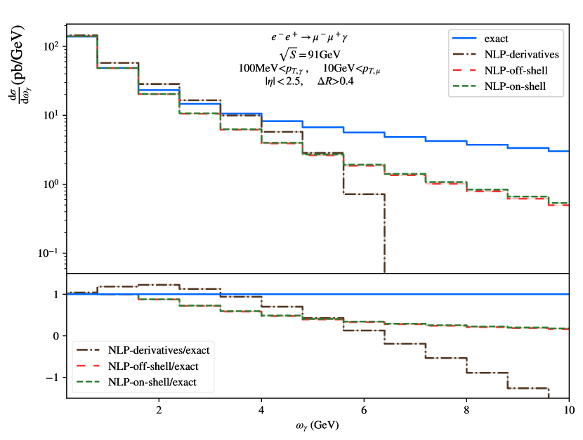
Figure 2: Comparison of the soft-photon energy spectra calculated using three formulations of the LBK theorem discussed in this paper with the exact (i.e. no soft expansion) result for the process $e^{-}e^{+}\to\mu^{-}\mu^{+}\gamma$ at $\sqrt{s}=91$ GeV.

We also see that the NLP approximations of the photon spectrum calculated using the non-radiative amplitude with momenta shifted on-shell or off-shell perform equally well for the photon energies considered here, indicating that the NNLP effects introduced in the on-shell shifts are not significant. Since the formulation with momenta shifted on-shell enables sourcing the amplitude subroutines from a wide range of public tools, we employ this formulation in further studies.

The NLP distributions in photon energy $\omega_{\gamma}$ and transverse momentum $p_{T,\gamma}$, obtained using the radiative amplitude with on-shell momenta eq. 2.40, are then compared to the LP and exact predictions in fig. 3 and fig. 4, respectively. In particular, we show distributions for very soft photons with 1 MeV$<\omega_{\gamma},\,p_{T,\gamma}<100$ MeV. As discussed above, the NLP formula relying on shifting momenta on-shell returns predictions which provide a very good approximation of the exact result. Up to the scale of 100 MeV, the difference between the two predictions is at a few per mille level and grows to a 1-2% level for $\omega_{\gamma}$ or $p_{T,\gamma}$ of up to ca. 1 GeV. In contrast, the LP approximation differs from the exact result by up to ca. 2% (6%) and up to ca. 40% (70%) in these two ranges of $\omega_{\gamma}$ ($p_{T,\gamma}$), correspondingly.

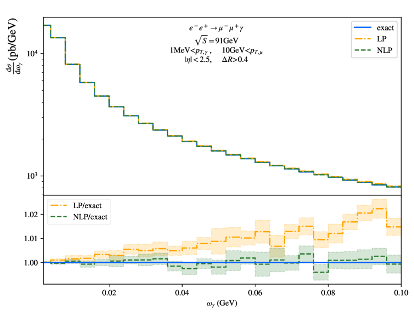
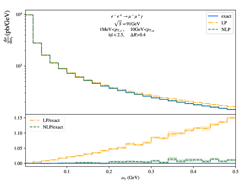
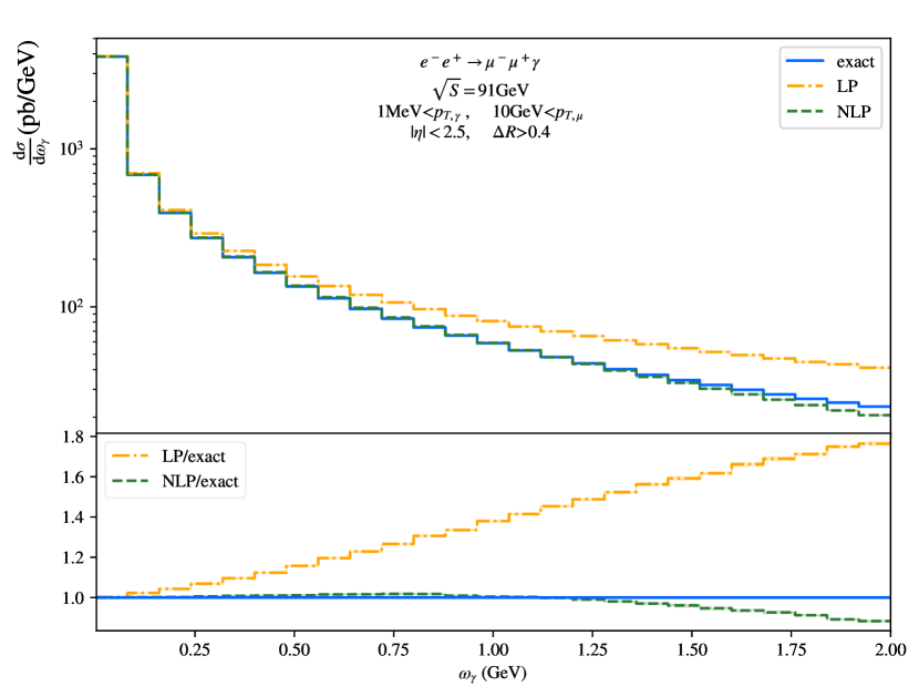
Figure 3: The $\mathrm{LP}$ and $\mathrm{NLP}$ approximations and the exact result for the energy spectrum of the photon in the $e^{-}e^{+}\to\mu^{-}\mu^{+}\gamma$ process at $\sqrt{s}=91$ GeV.

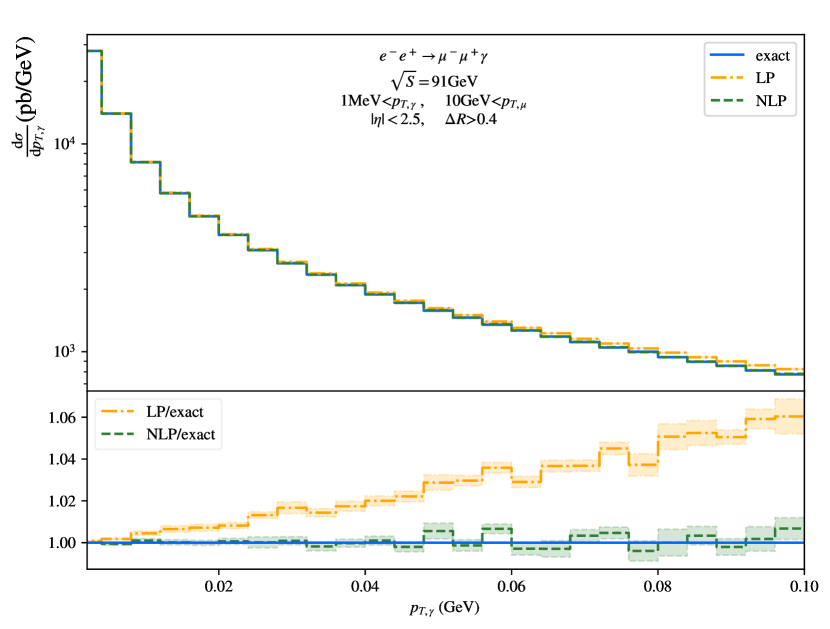
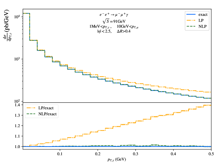
Figure 4: The $\mathrm{LP}$ and $\mathrm{NLP}$ approximations and the exact result for the transverse momentum spectrum of the photon in the $e^{-}e^{+}\to\mu^{-}\mu^{+}\gamma$ process at $\sqrt{s}=91$ GeV.

Next, we study the soft-photon spectra in the process $pp\to\mu^{+}\mu^{-}\gamma$. The differential distributions in photon energy and transverse momentum are shown in fig. 5 and fig. 6, respectively. The photon energy spectrum in fig. 5 is presented in both the partonic c.m. frame and the laboratory frame. No perceptible difference is observed between the results in the two frames for our choice of kinematical cuts. Perhaps not surprisingly, the behaviour of the LP and NLP approximations is very similar to the one found for the $e^{+}e^{-}$ collisions. Quantitatively, however, in the ranges of $\omega_{\gamma}$ and $p_{T,\gamma}$ studied here, the LP and NLP predictions appear to be relatively closer to the exact results than in the $e^{+}e^{-}$ case. To be more precise, within an accuracy of roughly $10\%$, the LP spectrum deviates from the exact result for $\omega_{\gamma}\gtrsim 400$MeV, $p_{T,\gamma}\gtrsim 150$MeV ($e^{+}e^{-}$) and $\omega_{\gamma}\gtrsim 1$GeV, $p_{T,\gamma}\gtrsim 500$MeV ($pp$). The NLP predictions reach this level of deviation only at $p_{T,\gamma}\gtrsim 1$ GeV in the $e^{+}e^{-}$ case, and at $p_{T,\gamma}\gtrsim 10$ GeV in the $pp$ case, i.e. outside of the soft regime.

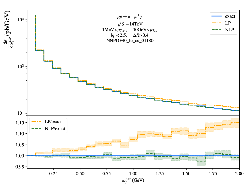
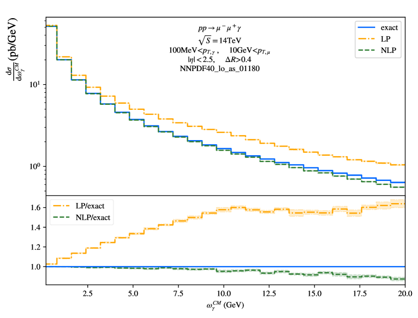
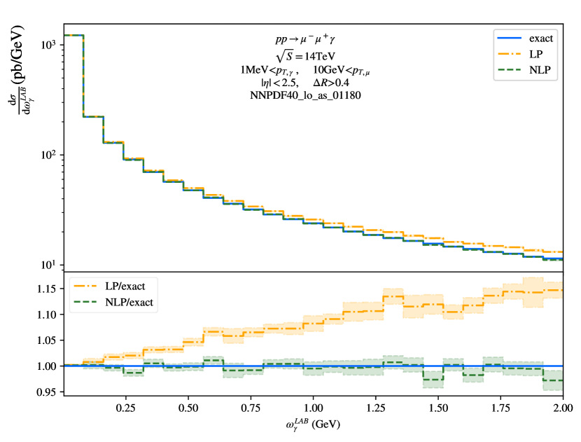
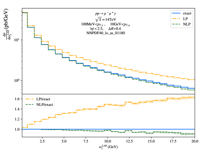
Figure 5: The $\mathrm{LP}$ and $\mathrm{NLP}$ approximations and the exact result for the energy spectrum of the photon in the partonic c.m. frame (top row) and the laboratory frame (bottom row) in the $pp\to\mu^{-}\mu^{+}\gamma$ process at $\sqrt{s}=14$ TeV.

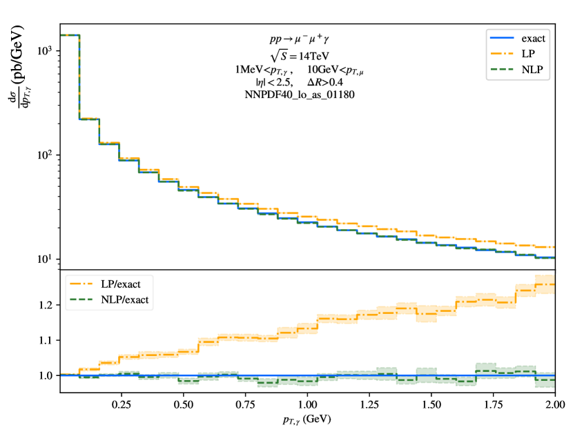
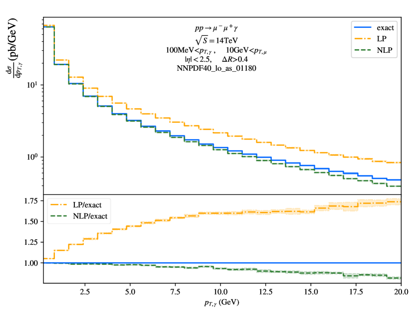
Figure 6: The $\mathrm{LP}$ and $\mathrm{NLP}$ approximations and the exact result for the transverse momentum spectrum of the photon in the $pp\to\mu^{-}\mu^{+}\gamma$ process at $\sqrt{s}=14$ TeV.

4 Conclusions

In this paper, we have presented an extensive study of the LBK theorem and its implications on numerical predictions for the soft-photon spectra.

First, motivated by recent discussions in the literature[35, 36, 37], we have addressed the consistency of the LBK theorem. As known for a long time, in the original formulation of the theorem[1] the non-radiative amplitude is calculated on a set of unphysical momenta. Seen in the most general way, this violation of momentum conservation leads to an ambiguity in the functional form of the non-radiative amplitude. We have provided a proof that the aforementioned ambiguity can only affect the expansion of the radiative amplitude starting from NNLP in soft-photon energy, i.e. beyond the formal accuracy of the LBK theorem, thus proving the validity of the LBK theorem at NLP. In doing so, we have generalized the remark by Burnett and Kroll by observing an invariance of the theorem at NLP under a specific transformation of the non-radiative amplitude. The consequence of this invariance is the presence of many equivalent forms of the LBK theorem, which include the original formulation by Low as one possibility.

Among the different versions of the theorem, for practical reasons, it is particularly attractive to consider those that restore momentum conservation in the calculation of the non-radiative amplitude. Such restoration can be achieved by reformulating the LBK theorem in terms of the non-radiative amplitude calculated on momenta which values are modified wrt. the momenta of the radiative amplitude. The modification that has been put forward in the literature [27, 67, 28] relies on adding small shifts of the order of the soft-photon momentum $k$. Apart from reviewing the derivation of the reformulated LBK theorem in terms of shifted momenta, we have proposed expressions for the momenta shifts which not only restore momentum conservation, but also ensure that each of the shifted momenta is on-shell. In this way, we facilitate the generation and numerical calculation of the non-radiative amplitude with a wide range of publicly available tools.

We have also studied the quality of the soft approximation provided by the LBK theorem in its various formulations on the example of the $e^{+}e^{-}\to\mu^{+}\mu^{-}\gamma$ process, analysed at LEP1 energies. We have found a remarkable improvement in the quality of the approximation for the formulations involving shifts w.r.t. the formulation of the theorem with derivatives, although we have considered the latter only for a specific form of the non-radiative amplitude. Depending on the required quality of the approximation, NNLP effects can be thus numerically relevant and the form of the LBK theorem used to calculate the NLP approximation of the soft-photon spectra needs to be chosen carefully. In this regard, our studies indicate that the formulations involving shifts should be preferred. Notably, for the implementation involving on-shell shifts, we have used the amplitudes generated by the MadGraph5 code, in this way demonstrating the feasibility of the calculations for a wide range of processes, given a corresponding phase-space integrating code is available.

Despite the long history of the LBK theorem, to the best of our knowledge, no study in the literature has explicitly identified when power-suppressed effects become visible in the soft-photon spectra. In order to address this question, we compared the exact, LP and NLP results for the $e^{+}e^{-}\to\mu^{+}\mu^{-}\gamma$ process at the LEP1 energy of $91$ GeV and the $pp\to\mu^{+}\mu^{-}\gamma$ process at the LHC energy of $14$ TeV. We have studied various ranges of photon energy and transverse momentum. For the cases studied here, the quality of the NLP approximation in a reasonably soft regime is of the order of, or better than, one percent, even though the specific results depend on the process, observable and the analysis set-up. The quality of the LP approximation is significantly worse, meaning that for measurements where a precision of a few percent can be reached in the soft regime, the LP might not provide a good enough approximation. Correspondingly, our results suggest that in order to access the power-suppressed terms, a percent-level precision is needed, especially in the case of the $pp\to\mu^{+}\mu^{-}\gamma$ process at the LHC. Obviously, this is only a crude estimate. A more precise statement would require a careful analysis of all theoretical and experimental uncertainties.

The results of this work open up the possibility of many follow-up analyses. The two processes we studied here involve simple leptonic final states and central rapidity photons. Given that the excess in the soft-photon spectrum was observed for $e^{+}e^{-}$ collisions in hadronic final states, it would be interesting to investigate the impact of NLP corrections on the predictions for the associated photon production with jets. In this regard, it would also be interesting to extend the analysis by including QCD corrections at 1-loop[28], which will be relevant for both initial and final state hadrons. In the long run, the studies need to be extended to $pp$ collisions resulting in various hadronic final states with photons at forward rapidities, as planned to be investigated with the ALICE 3 detector[66].

Appendix A Case study: $2\to 2$ scattering

In this section we apply the general arguments of Section 2.2 concerning the traditional form of the LBK theorem with derivatives to the simple case of photon bremsstrahlung in pion scattering. In doing so, we compare with the analysis of Lebiedowicz, Nachmann, Szczurek (LNS) [35], showing that their result is equivalent to the traditional form of the LBK theorem and with previous studies in the literature.

A.1 LBK theorem for $\pi^{-}\pi^{0}\to\pi^{-}\pi^{0}\gamma$

Following [1] and [35], and using the notation established in [35], we consider the following process:

$$\pi^{-}(p_{a})\pi^{0}(p_{b})\to\pi^{-}(p^{\prime}_{1})\pi^{0}(p^{\prime}_{2})\gamma(k)~{},$$

with

$$p_{a}+p_{b}=p^{\prime}_{1}+p^{\prime}_{2}+k~{}.$$

For this process, the LBK theorem in the form of eq. 2.7, adapted to the case of scalar particles, reads

$$\mathcal{A}^{\mu}(p_{a},p_{b},p^{\prime}_{1},p^{\prime}_{2},k) =e\left[\frac{p_{a}^{\mu}}{k\cdot p_{a}}\mathcal{H}(p_{a},p_{b},p^{\prime}_{1},p^{\prime}_{2})+G_{a}^{\mu\nu}\partialderivative{\mathcal{H}(p_{a},p_{b},p^{\prime}_{1},p^{\prime}_{2})}{p_{a}^{\nu}}\right]$$

$$\phantom{=}-e\left[\frac{p_{1}^{\prime\mu}}{k\cdot p^{\prime}_{1}}\mathcal{H}(p_{a},p_{b},p^{\prime}_{1},p^{\prime}_{2})-G_{1}^{\mu\nu}\partialderivative{\mathcal{H}(p_{a},p_{b},p^{\prime}_{1},p^{\prime}_{2})}{p_{1}^{\prime\nu}}\right]+\order{k}$$

$$=e\left[\frac{p_{a}^{\mu}}{k\cdot p_{a}}-\frac{p_{1}^{\prime\mu}}{k\cdot p^{\prime}_{1}}+G_{a}^{\mu\nu}\partialderivative{p_{a}^{\nu}}+G_{1}^{\mu\nu}\partialderivative{p^{\prime\nu}_{1}}\right]\mathcal{H}(p_{a},p_{b},p^{\prime}_{1},p^{\prime}_{2})+\order{k}~{}.$$ (A.1)

To show the ambiguity in the calculation of the non-radiative amplitude with radiative kinematics, we consider the following two choices for $\mathcal{H}$:

$$\mathcal{H}_{1}=\mathcal{H}(s^{\prime}_{L},t_{1}),\qquad\mathcal{H}_{2}=\mathcal{H}(s^{\prime}_{L},t_{2})~{},$$ (A.2)

where we defined

$$s^{\prime}_{L}=p_{a}\cdot p_{b}+p^{\prime}_{1}\cdot p^{\prime}_{2},\qquad t_{1}=(p_{a}-p^{\prime}_{1})^{2},\qquad t_{2}=(p_{b}-p^{\prime}_{2})^{2}.$$ (A.3)

Here, $\mathcal{H}(s_{L},t)$ is the amplitude for the non-radiative process $\pi^{-}(p_{a})\pi^{0}(p_{b})\to\pi^{-}(p_{1})\pi^{0}(p_{2})$. Obviously, $p_{a}+p_{b}=p_{1}+p_{2}$, so in the elastic limit $t_{1}=(p_{a}-p_{1})^{2}$ and $t_{2}=(p_{b}-p_{2})^{2}$, hence we have $t_{1}=t_{2}$, and thus $\mathcal{H}_{1}=\mathcal{H}_{2}$.

Now we consider

$$\partialderivative{\mathcal{H}_{i}}{p_{a}^{\nu}} =\partialderivative{\mathcal{H}_{i}}{s^{\prime}_{L}}\partialderivative{s^{\prime}_{L}}{p_{a}^{\nu}}+\partialderivative{\mathcal{H}_{i}}{t_{i}}\partialderivative{t_{i}}{p_{a}^{\nu}},$$

$$\partialderivative{\mathcal{H}_{i}}{p^{\prime\nu}_{1}} =\partialderivative{\mathcal{H}_{i}}{s^{\prime}_{L}}\partialderivative{s^{\prime}_{L}}{p^{\prime\nu}_{1}}+\partialderivative{\mathcal{H}_{i}}{t_{i}}\partialderivative{t_{i}}{p^{\prime\nu}_{1}}~{},$$ (A.4)

where no sum over the index $i=1,2$ has been assumed. The derivatives of $s^{\prime}_{L}$ in eq. A.4 read

$$\partialderivative{s^{\prime}_{L}}{p_{a}^{\nu}}=p_{b\nu},\qquad\partialderivative{s^{\prime}_{L}}{p^{\prime\nu}_{1}}=p^{\prime}_{2\nu}~{}.$$

The terms with derivatives of $t_{i}$ are different for $i=1,2$, and are given by

$$\partialderivative{t_{1}}{p^{\nu}_{a}}=2(p_{a}-p^{\prime}_{1})_{\nu},\qquad\partialderivative{t_{1}}{p^{\prime\nu}_{1}}=-2(p_{a}-p^{\prime}_{1})_{\nu},\qquad\partialderivative{t_{2}}{p^{\nu}_{a}}=\partialderivative{t_{2}}{p^{\prime\nu}_{1}}=0~{}.$$ (A.5)

Putting the above equations together we obtain two seemingly distinct forms for the LBK theorem, depending on whether we take ${\cal H}={\cal H}_{1}$ or ${\cal H}={\cal H}_{2}$ in eq. A.1. They read

$$\mathcal{A}^{\mu}(p_{a},p_{b},p^{\prime}_{1},p^{\prime}_{2},k)=e\Bigg{[} \left(\frac{p_{a}^{\mu}}{k\cdot p_{a}}-\frac{p_{1}^{\prime\mu}}{k\cdot p^{\prime}_{1}}\right)+\left(p_{b}^{\mu}-\frac{p_{b}\cdot k}{p_{a}\cdot k}p_{a}^{\mu}+p^{\prime\mu}_{2}-\frac{p^{\prime}_{2}\cdot k}{p^{\prime}_{1}\cdot k}p^{\prime\mu}_{1}\right)\partialderivative{s^{\prime}_{L}}$$

$$-2(p_{a}-p^{\prime}_{1})\cdot k\left(\frac{p_{a}^{\mu}}{k\cdot p_{a}}-\frac{p_{1}^{\prime\mu}}{k\cdot p^{\prime}_{1}}\right)\partialderivative{t_{1}}\Bigg{]}\mathcal{H}_{1}+\order{k}~{},$$

$$\mathcal{A}^{\mu}(p_{a},p_{b},p^{\prime}_{1},p^{\prime}_{2},k)=e\Bigg{[} \left(\frac{p_{a}^{\mu}}{k\cdot p_{a}}-\frac{p_{1}^{\prime\mu}}{k\cdot p^{\prime}_{1}}\right)$$

$$+\left(p_{b}^{\mu}-\frac{p_{b}\cdot k}{p_{a}\cdot k}p_{a}^{\mu}+p^{\prime\mu}_{2}-\frac{p^{\prime}_{2}\cdot k}{p^{\prime}_{1}\cdot k}p^{\prime\mu}_{1}\right)\partialderivative{s^{\prime}_{L}}\Bigg{]}\mathcal{H}_{2}+\order{k}~{}.$$ (A.6)

If one ignores the fact that $\mathcal{H}_{1}$ and $\mathcal{H}_{2}$ are not the same, the two expressions indeed yield different results, thus seemingly invalidating the LBK theorem. However, by relating $\mathcal{H}_{1}$ and $\mathcal{H}_{2}$, the difference disappears at NLP. In fact, one has

$$\mathcal{H}_{2}=\mathcal{H}(s^{\prime}_{L},t_{2})=\mathcal{H}(s^{\prime}_{L},t_{1})+(t_{2}-t_{1})\partialderivative{\mathcal{H}(s^{\prime}_{L},t_{1})}{t_{1}}+\order{k^{2}}~{}.$$ (A.7)

Using then the expression

$$t_{2}-t_{1}=(p_{b}-p^{\prime}_{2})^{2}-(p_{a}-p^{\prime}_{1})^{2}=(p_{a}-p^{\prime}_{1}-k)^{2}-(p_{a}-p^{\prime}_{1})^{2}=-2k\cdot(p_{a}-p^{\prime}_{1})+\order{k^{2}}~{},$$ (A.8)

we get

$$\mathcal{H}_{2}=\mathcal{H}_{1}-2k\cdot(p_{a}-p^{\prime}_{1})\partialderivative{\mathcal{H}_{1}}{t_{1}}+\order{k^{2}}~{},$$ (A.9)

which accounts for the difference between the two previous expressions. This is the cancellation we saw in Section 2.2, where we proved it in the general case.

A.2 Comparison between LNS and the original work of Low

The soft bremsstrahlung in pion scattering has been computed also by the authors of ref. [35]. Their final result, which is given by eq. (3.27) of their paper, reads

$$\mathcal{A}^{\mu}= e\mathcal{H}(s_{L},t)\left[\frac{p_{a}^{\mu}}{p_{a}\cdot k}-\frac{p^{\prime\mu}_{1}}{p^{\prime}_{1}\cdot k}\right]+2e\partialderivative{\mathcal{H}(s_{L},t)}{s_{L}}\left[p_{b}^{\mu}-\frac{p_{b}\cdot k}{p_{a}\cdot k}p_{a}^{\mu}\right]$$

$$-2e\partialderivative{\mathcal{H}(s_{L},t)}{t}\left[(p_{a}-p_{1})\cdot k-p_{a}\cdot l_{1}\right]\left[\frac{p_{a}^{\mu}}{p_{a}\cdot k}-\frac{p^{\mu}_{1}}{p_{1}\cdot k}\right]+\order{k}~{},$$ (A.10)

where the non-radiative amplitude $\cal H$ is written as a function of the two variables $s_{L}$ and $t$

$$s_{L}=p_{a}\cdot p_{b}+p_{1}\cdot p_{2},\qquad t=(p_{a}-p_{1})^{2}=(p_{b}-p_{2})^{2}.$$ (A.11)

The momenta fulfill the relations

$$p_{a}+p_{b}=p_{1}+p_{2}=p^{\prime}_{1}+p^{\prime}_{2}+k$$ (A.12)

and $l_{i}$ are defined as a shift between $p$ and $p^{\prime}$ as follows:

$$l_{i}=p_{i}-p^{\prime}_{i}.$$ (A.13)

As done in [1], here we set $k^{2}=0$ and drop all terms proportional to $k^{\mu}$ since we assume all final states to be on-shell.

The authors of [35] compare then Section A.2 to the one derived by Low in ref. [1], which they report in eq. (3.29) of their paper. It reads

$$\tilde{\mathcal{A}}^{\mu}=e\mathcal{H}(s_{L},t)\left[\frac{p_{a}^{\mu}}{p_{a}\cdot k}-\frac{p^{\mu}_{1}}{p_{1}\cdot k}\right]+e\partialderivative{\mathcal{H}(s_{L},t)}{s_{L}}\left[p_{b}^{\mu}-\frac{p_{b}\cdot k}{p_{a}\cdot k}p_{a}^{\mu}+p_{2}^{\mu}-\frac{p_{2}\cdot k}{p_{1}\cdot k}p_{1}^{\mu}\right]+\order{k}~{}.$$ (A.14)

They conclude that, while the LP terms agree, there is a discrepancy in the NLP terms. We first point out that (A.14) does not precisely coincide with the result given by Low in equation (2.16) of [1]. In fact, by looking at eq. (2.1) and eq. (2.16) in [1], one concludes that the correct expression should be

$$\mathcal{A}^{\mu}=e\mathcal{H}(s^{\prime}_{L},t_{2})\left[\frac{p_{a}^{\mu}}{p_{a}\cdot k}-\frac{p^{\prime\mu}_{1}}{p^{\prime}_{1}\cdot k}\right]+e\partialderivative{\mathcal{H}(s^{\prime}_{L},t_{2})}{s^{\prime}_{L}}\left[p_{b}^{\mu}-\frac{p_{b}\cdot k}{p_{a}\cdot k}p_{a}^{\mu}+p^{\prime\mu}_{2}-\frac{p^{\prime}_{2}\cdot k}{p^{\prime}_{1}\cdot k}p^{\prime\mu}_{1}\right]+\order{k}~{},$$ (A.15)

with $s^{\prime}_{L}$ and $t_{2}$ defined as in eq. A.3. This form of the LBK theorem is indeed what we obtained in eq. A.6.

A careful comparison of expressions Section A.2 and eq. A.15 shows that they are in perfect agreement with each other, up to $\order{k}$. To simplify the comparison, it is worth noticing that $p$ and $p^{\prime}$ are equal up to $\order{k}$ corrections. Therefore, to order $\order{k}$, the difference between $p$ and $p^{\prime}$ is only relevant for the first term, and eq. A.15 can be rewritten as

$$\mathcal{A}^{\mu}=e\mathcal{H}(s^{\prime}_{L},t_{2})\left[\frac{p_{a}^{\mu}}{p_{a}\cdot k}-\frac{p^{\prime\mu}_{1}}{p^{\prime}_{1}\cdot k}\right]+e\partialderivative{\mathcal{H}(s_{L},t)}{s_{L}}\left[p_{b}^{\mu}-\frac{p_{b}\cdot k}{p_{a}\cdot k}p_{a}^{\mu}+p^{\mu}_{2}-\frac{p_{2}\cdot k}{p_{1}\cdot k}p^{\mu}_{1}\right]+\order{k}~{}.$$ (A.16)

To compare Section A.2 with eq. A.16 it is necessary to use the formula

$$\mathcal{H}(s^{\prime}_{L},t_{2})=\mathcal{H}(s_{L},t)+\delta s^{\prime}_{L}\partialderivative{\mathcal{H}}{s_{L}}+\delta t_{2}\partialderivative{\mathcal{H}}{t}~{},$$ (A.17)

where we defined

$$\delta s^{\prime}_{L} =s^{\prime}_{L}-s_{L}=p^{\prime}_{1}\cdot p^{\prime}_{2}-p_{1}\cdot p_{2}=(p_{1}-l_{1})\cdot(p_{2}-l_{2})-p_{1}\cdot p_{2}$$

$$=-(l_{1}\cdot p_{2}+l_{2}\cdot p_{1})+\order{k^{2}}=-(p_{1}+p_{2})\cdot k+\order{k^{2}}$$

$$=-(p_{a}+p_{b})\cdot k+\order{k^{2}}~{},$$

$$\delta t_{2} =t_{2}-t=(p_{b}-p^{\prime}_{2})^{2}-(p_{b}-p_{2})^{2}=(p_{b}-p_{2}+l_{2})^{2}-(p_{b}-p_{2})^{2}$$

$$=2l_{2}\cdot(p_{b}-p_{2})+\order{k^{2}}=-2(k-l_{1})\cdot(p_{a}-p_{1})+\order{k^{2}}$$

$$=-2\left[(p_{a}-p_{1})\cdot k-p_{a}\cdot l_{1}\right]+\order{k^{2}}~{}.$$ (A.18)

Here we used the relations $p_{1}\cdot l_{2}=p_{1}\cdot k$ and $p_{2}\cdot l_{1}=p_{2}\cdot k$, which can be derived from the two relations $l_{1}+l_{2}=k$ and $p_{i}\cdot l_{i}=0$ (i.e. eq. (3.17) and eq. (3.22) in [35]).

Inserting now eq. A.17 into eq. A.16, we see that the term proportional to $\mathcal{H}$ is identical to the one in Section A.2. Additionally, the term proportional to $\partialderivative{\mathcal{H}}{t}$ is given by

$$e\delta t_{2}\partialderivative{\mathcal{H}}{t}\left[\frac{p_{a}^{\mu}}{p_{a}\cdot k}-\frac{p^{\prime\mu}_{1}}{p^{\prime}_{1}\cdot k}\right]=-2e\partialderivative{\mathcal{H}}{t}\left[(p_{a}-p_{1})\cdot k-p_{a}\cdot l_{1}\right]\left[\frac{p_{a}^{\mu}}{p_{a}\cdot k}-\frac{p^{\prime\mu}_{1}}{p^{\prime}_{1}\cdot k}\right]~{}.$$ (A.19)

The r.h.s. of eq. A.19 coincides with the third term in Section A.2 after dropping the prime in the last parenthesis (this is possible because this term is already a NLP term, and thus the difference due to replacing $p$ with $p^{\prime}$ is a NNLP effect). Finally, the term proportional to $\partialderivative{\mathcal{H}}{s_{L}}$ has now the following expression

$$e\delta s^{\prime}_{L}\partialderivative{\mathcal{H}}{s_{L}}\left[\frac{p_{a}^{\mu}}{p_{a}\cdot k}-\frac{p^{\mu}_{1}}{p_{1}\cdot k}\right]+e\partialderivative{\mathcal{H}}{s_{L}}\left[p_{b}^{\mu}-\frac{p_{b}\cdot k}{p_{a}\cdot k}p_{a}^{\mu}+p^{\mu}_{2}-\frac{p_{2}\cdot k}{p_{1}\cdot k}p^{\mu}_{1}\right]~{},$$ (A.20)

where again the prime in the first term can dropped because $\delta s^{\prime}_{L}$ is already of order $\order{k}$. After some algebra, it is easy to show that this term reads

$$2e\partialderivative{\mathcal{H}}{s_{L}}\left[p_{b}^{\mu}-k\cdot p_{b}\frac{p_{a}^{\mu}}{p_{a}\cdot k}\right]~{},$$ (A.21)

in perfect agreement with the second term in Section A.2. Therefore, the LNS result (Section A.2) and Low’s original result (eq. A.15) are completely equivalent at NLP.

We note also that although here we focused on pion scattering, we expect analogous arguments to hold for the proton scattering discussed in [37, 36].

A.3 Comparison between LNS and other literature

A comparison between the result of LNS, i.e. Section A.2, and the previous literature has been carried out in the appendix of [35]. It is claimed there that all previous known forms of the LBK theorem are problematic. In particular, LNS claim that the result of reference [24] is not consistent, since it depends on an arbitrary quantity, as discussed below. However, a careful analysis shows that this claim has no valid foundation, since the dependence on such quantity vanishes.

The argument in [35] is the following. In [24] Low’s theorem is written in a form that depends on the following four quantities:

$$I_{1} =\left(-l_{1}\cdot\partialderivative{p_{1}}-l_{2}\cdot\partialderivative{p_{2}}-k\cdot\partialderivative{p_{a}}\right)\mathcal{H}(p_{a},p_{b},p_{1},p_{2})~{},$$

$$I_{2} =\left(-l_{1}\cdot\partialderivative{p_{1}}-l_{2}\cdot\partialderivative{p_{2}}+k\cdot\partialderivative{p_{1}}\right)\mathcal{H}(p_{a},p_{b},p_{1},p_{2})~{},$$

$$I_{3}^{\mu} =\partialderivative{\mathcal{H}(p_{a},p_{b},p_{1},p_{2})}{p_{a\mu}},\qquad I_{4}^{\mu}=\partialderivative{\mathcal{H}(p_{a},p_{b},p_{1},p_{2})}{p_{1\mu}}~{}.$$ (A.22)

If one then restricts the analysis to an amplitude $\mathcal{H}$ that depends solely on the quantity $p_{a}^{2}+p_{1}^{2}-p_{b}^{2}-p_{2}^{2}$, as done in [35], the elastic amplitude is given by a constant, since

$$\mathcal{H}(p_{a},p_{b},p_{1},p_{2})=f(p_{a}^{2}+p_{1}^{2}-p_{b}^{2}-p_{2}^{2})=f(m_{a}^{2}+m_{1}^{2}-m_{b}^{2}-m_{2}^{2})\equiv f_{0}.$$ (A.23)

Thus, the derivatives of the elastic amplitude vanish and the final result only depends on the value of $f_{0}$. However, if one considers the corresponding expressions in eq. A.22, they become

$$I_{1}=-2(k\cdot p_{a})f^{\prime}_{0},\qquad I_{2}=2(k\cdot p_{1})f^{\prime}_{0},\qquad I_{3}^{\mu}=2p_{a}^{\mu}f^{\prime}_{0},\qquad I_{4}^{\mu}=2p_{1}^{\mu}f^{\prime}_{0}~{}.$$ (A.24)

Therefore, in eq. A.24 there is a dependence on $f^{\prime}_{0}$ (the derivative of $f$ evaluated on non-radiative momenta). $f^{\prime}_{0}$ is an arbitrary quantity, which seems to invalidate the consistency of the result in [24].

To see why this argument does not imply an inconsistency of the LBK theorem in the form given in ref. [24], a more detailed analysis of the complete expressions is needed. A direct comparison between [24] and [35] is unfortunately not possible, since the processes under consideration are different ($e^{-}\pi^{0}\to e^{-}\pi^{0}$ for ref. [24], and $\pi^{-}\pi^{0}\to\pi^{-}\pi^{0}$ for LNS). The comparison thus requires a dictionary to relate the theorems with fermions and scalar fields, respectively, which is summarized in Table 1.

Gervais	Lebiedowicz, Nachtmann, Szczurek
$\frac{1}{\not{p}-m}$	$\frac{1}{p^{2}-m^{2}}$
$\gamma_{\mu}$	$p_{\mu}+p^{\prime}_{\mu}$
$u,v,\bar{u},\bar{v}$	$1$
$p_{1}$, $p^{\prime}_{1}$	$p_{a}$
$k_{1}$, $k^{\prime}_{1}$	$p_{b}$
$p_{2}$	$p^{\prime}_{1}$
$k_{2}$	$p^{\prime}_{2}$
$p^{\prime}_{2}$	$p_{1}$
$k^{\prime}_{2}$	$p_{2}$
$q$	$k$
$\eta_{1}$, $\xi_{1}$	0
$\xi_{2}$	$-l_{1}$
$\eta_{2}$	$-l_{2}$

Table 1: Relation between the notations used in [24] and [35].

After carefully taking this translation into account, Low’s theorem in the notation of ref. [24] (see equation (20) there) reads

$$\mathcal{A}^{\mu}=e\left(\frac{p_{1}^{\prime\mu}}{p^{\prime}_{1}\cdot k}-\frac{p_{a}^{\mu}}{p_{a}\cdot k}\right)\mathcal{H}(p_{a},p_{b},p_{1},p_{2})-e\left(\frac{p_{a}^{\mu}}{p_{a}\cdot k}I_{1}-\frac{p_{1}^{\mu}}{p_{1}\cdot k}I_{2}+I_{3}^{\mu}+I_{4}^{\mu}\right)~{}.$$ (A.25)

In particular, it is worth noting that the expression for $I_{i}$ in eq. A.25 enter via the following combinations

$$p_{a}^{\mu}I_{1}+(p_{a}\cdot k)I^{\mu}_{3},\qquad p_{1}^{\mu}I_{2}-(p_{1}\cdot k)I_{4}^{\mu}~{}.$$ (A.26)

Therefore, after inserting the expressions of eq. A.24 in eq. A.25, the dependence on $f_{0}^{\prime}$ vanishes. Hence, for the case of eq. A.23 studied in this section, eq. A.25 is consistent with other formulations of the LBK theorem, such as LNS (Section A.2) and Low’s (eq. A.15).

Appendix B LBK invariance under momenta transformation

We consider here the invariance under eq. 2.17 in the case where $\Delta$ arises from linear transformations of the momenta in $\cal H$. Specifically, we prove that, at NLP, eq. 2.16 is invariant under the following transformation,

$${\cal H}(p_{1},\dots,p_{n})\to{\cal H}(\tilde{p}_{1},\dots,\tilde{p}_{n})~{},$$ (B.1)

with

$$\tilde{p}_{i}(k)=p_{i}+c_{i}k+\order{k^{2}},$$ (B.2)

where the coefficients $c_{i}$ are arbitrary. To verify the invariance, let us apply eq. B.1 to eq. 2.16. We get

$$\overline{|{\cal A}(p_{1},\dots,p_{n},k)|}^{2} =\sum_{ij=1}^{n}(-\eta_{i}\eta_{j}Q_{i}Q_{j})\frac{p_{i}\cdot p_{j}}{p_{i}\cdot k\,p_{j}\cdot k}\overline{|{\cal H}(\tilde{p}_{1},\dots,\tilde{p}_{n})|}^{2}$$

$$\quad+\sum_{ij=1}^{n}(-\eta_{i}\eta_{j}Q_{i}Q_{j})\frac{p_{i\,\mu}}{p_{i}\cdot k}\eta_{j}\left(g^{\mu\nu}-\frac{p^{\mu}_{j}k^{\nu}}{p_{j}\cdot k}\right)\frac{d}{dp_{j}^{\nu}}\overline{|{\cal H}(\tilde{p}_{1},\dots,\tilde{p}_{n})|}^{2}~{},$$ (B.3)

where partial derivatives have been replaced with total derivatives due to the non-trivial functional dependence inside the non-radiative amplitude. The function $\overline{|\cal H|}^{2}$ can be simply expanded in $k$ by using the functional dependence of eq. B.2, to get

$$\overline{|{\cal H}(\tilde{p}_{1},\dots,\tilde{p}_{n})|}^{2}=\overline{|{\cal H}(p_{1},\dots,p_{n})|}^{2}+k^{\mu}\sum_{i}c_{i}\frac{\partial}{\partial p_{i}^{\mu}}\overline{|{\cal H}(p_{1},\dots,p_{n})|}^{2}+\order{k^{2}}~{}.$$ (B.4)

To proceed further, we note that so far momentum conservation has not been imposed. We can do so by making the dependence over the momenta $p_{i}$ explicit in the soft momentum, i.e. by enforcing $k^{\mu}\to k^{\mu}(p_{1},\dots,p_{n})=\sum_{i}\eta_{i}p_{i}^{\mu}$. Subsequently, by differentiating eq. B.4 we get

$$\frac{d}{dp_{j}^{\nu}}\overline{|{\cal H}(\tilde{p}_{1},\dots,\tilde{p}_{n})|}^{2} =\frac{\partial}{\partial p_{j}^{\nu}}\overline{|{\cal H}(p_{1},\dots,p_{n})|}^{2}+\delta_{\nu}^{\mu}\eta_{j}\sum_{i}c_{i}\frac{\partial}{\partial p^{\mu}_{i}}\overline{|{\cal H}(p_{1},\dots,p_{n})|}^{2}+{\mathcal{O}}(k)~{}.$$ (B.5)

Note that since eq. B.4 is expanded up to $\order{k^{2}}$, we have to truncate eq. B.5 to $\order{k}$ because differentiating $k$ w.r.t the momenta $p_{i}$ reduces the order of the expansion. In particular, $\frac{d\order{k^{2}}}{dp_{j}^{\nu}}=\order{k}$. This is not a problem, since the l.h.s. of eq. B.5 is multiplied by an expression which is suppressed w.r.t. the other term in eq. B.3 by one power of $k$. Therefore, plugging eq. B.4 and eq. B.5 into eq. B.3 we get

$$\overline{|{\cal A}(p_{1},\dots,p_{n},k)|}^{2}= \sum_{ij=1}^{n}(-\eta_{i}\eta_{j}Q_{i}Q_{j})\frac{p_{i}\cdot p_{j}}{p_{i}\cdot k\,p_{j}\cdot k}\overline{|{\cal H}(p_{1},\dots,p_{n})|}^{2}$$

$$+\sum_{ij=1}^{n}(-\eta_{i}\eta_{j}Q_{i}Q_{j})\frac{p_{i\,\mu}}{p_{i}\cdot k}\eta_{j}\left(g^{\mu\nu}-\frac{p^{\mu}_{j}k^{\nu}}{p_{j}\cdot k}\right)\frac{\partial}{\partial p_{j}^{\nu}}\overline{|{\cal H}(p_{1},\dots,p_{n})|}^{2}$$

$$+R(c_{i})~{},$$ (B.6)

where

$$R(c_{i}) =\sum_{ij=1}^{n}(-\eta_{i}\eta_{j}Q_{i}Q_{j})\frac{p_{i}\cdot p_{j}}{p_{i}\cdot k\,p_{j}\cdot k}k^{\mu}\sum_{m}c_{m}\frac{\partial}{\partial p^{\mu}_{m}}\overline{|{\cal H}(p_{1},\dots,p_{n})|}^{2}$$

$$\quad+\sum_{ij=1}^{n}(-\eta_{i}\eta_{j}Q_{i}Q_{j})\frac{p^{i}_{\mu}}{p_{i}\cdot k}\eta_{j}\left(g^{\mu\nu}-\frac{p^{\mu}_{j}k^{\nu}}{p_{j}\cdot k}\right)\eta_{j}\sum_{m}c_{m}\frac{\partial}{\partial p^{\nu}_{m}}\overline{|{\cal H}(p_{1},\dots,p_{n})|}^{2}+{\cal O}(1)~{}.$$ (B.7)

To prove the invariance of eq. 2.16 under eq. B.1 at NLP, we have to show that the remainder term $R(c_{i})$, which depends on the arbitrary coefficients $c_{i}$, is ${\cal O}(1)$ (i.e. NNLP). This follows straightforwardly by first noting that, thanks to $\eta^{2}_{j}=1$, the term in the first line of eq. B.7 cancels with the analogous term in the second line. The term proportional to $g^{\mu\nu}$ then vanishes since $\sum_{j}\eta_{j}Q_{j}=0$ by charge conservation, thus leaving $R(c_{i})={\cal O}(1)$, as desired.

Having established that the LBK theorem in the form of eq. 2.16 is invariant under eq. B.1 at NLP, the consistency of the theorem (i.e. the possibility to evaluate $\cal H$ on a set of unphysical momenta as in eq. 2.16) follows as a corollary. In fact, the invariance under eq. B.1 guarantees that at NLP there is an infinite number of equivalent forms of the theorem, one for each choice of the coefficients $c_{i}$. In particular, the unphysical momenta of eq. 2.16 corresponds to the trivial transformation with $c_{i}=0$. On the other hand, we can choose $c_{i}$ so that momentum conservation for non-radiative amplitude is restored (as in the strategy of Burnett and Kroll), i.e.

$$\sum_{i}\eta_{i}c_{i}=-1~{},\qquad\sum_{i}\eta_{i}\tilde{p}_{i}=0~{}.$$ (B.8)

Therefore, the form of the theorem in eq. 2.16 where $\cal H$ is evaluated on a set of unphysical momenta is equivalent, up to NNLP corrections, to the form where momentum conservation is restored (and thus no ambiguity is present).

Note that although the argument presented in this appendix is quite general, it fails when the invariance of the amplitude cannot be represented by linear shifts. A simple example is given by a constant amplitude that does not depend on the external momenta. In that case, for the consistency of eq. 2.16 one has to rely on the more general argument of Section 2.2.

Appendix C Calculation of the modified shifts

We show here the calculation that leads to the expression in eq. 2.40. We consider the conditions (i)-(iii) of eq. 2.36, eq. 2.37 and eq. 2.38. The most general form for $\delta p_{i}$ reads

$$\delta p_{i}^{\mu}=\sum_{j}A_{ij}^{\mu\nu}p_{j\nu}+B_{i}^{\mu\nu}k_{\nu}.$$ (C.1)

However, it is enough for our purposes to consider

$$\delta p_{i}^{\mu}=\sum_{j}A_{ij}p_{j}^{\mu}+B_{i}k^{\mu}.$$ (C.2)

We can further restrict our ansatz by assuming the set $\{p_{i}^{\mu},k^{\mu}\}$ to be linearly independent. Although clearly not true in general, this is not a problem since we are only interested in finding a single solution. With this assumption, we can now insert eq. C.2 into eq. 2.36, eq. 2.37 and eq. 2.38 to determine the coefficients $A_{ij}$ and $B_{i}$. We get

1. $$\sum_{i,j}\eta_{i}A_{ij}p_{j}^{\mu}+\left(\sum_{i}\eta_{i}B_{i}+1\right)k^{\mu}=0~{},$$ (C.3)

   which gives

   $$\sum_{i}\eta_{i}A_{ij}=0,\quad\sum_{i}\eta_{i}B_{i}=-1~{}.$$ (C.4)

2. $$\left(\sum_{j}\left(\delta_{ij}+A_{ij}\right)p_{j}^{\mu}+B_{i}k^{\mu}\right)^{2}=m^{2}~{},$$ (C.5)

   which gives

   $$\sum_{j,k}\left(2\delta_{ij}A_{ik}+A_{ij}A_{ik}\right)(p_{j}\cdot p_{k})+2\sum_{j}\left(\delta_{ij}B_{i}+A_{ij}B_{i}\right)(p_{j}\cdot k)=0~{}.$$ (C.6)

3. $$A_{ij} =-Q_{i}\left(\overline{\left|{\cal S}_{\text{LP}}\right|}^{2}\right)^{-1}\frac{\eta_{j}Q_{j}}{k\cdot p_{j}}+\order{k^{2}}~{},$$

   $$B_{i} =Q_{i}\left(\overline{\left|{\cal S}_{\text{LP}}\right|}^{2}\right)^{-1}\sum_{j}\left(\frac{\eta_{j}Q_{j}}{k\cdot p_{j}}\right)\frac{p_{j}\cdot p_{i}}{p_{i}\cdot k}+\order{k}=-\sum_{j}A_{ij}\frac{p_{i}\cdot p_{j}}{p_{i}\cdot k}+\order{k}~{}.$$ (C.7)

As we can see, the conditions given by eq. C.4, eq. C.6 and eq. C.7 are not too restrictive. Thus, we still have the freedom to select a single solution by introducing a scalar coefficient $A$ such that we have

$$A_{ij}=AQ_{i}\frac{\eta_{j}Q_{j}}{k\cdot p_{j}}~{}.$$ (C.8)

Then, the condition $\sum_{i}\eta_{i}A_{ij}=0$ is immediately satisfied by charge conservation. The remaining conditions now yield

$$\sum_{i}\eta_{i}B_{i}=-1~{},$$ (C.9)

$$2AQ_{i}\sum_{j}\eta_{j}Q_{j}\frac{p_{i}\cdot p_{j}}{k\cdot p_{j}}-A^{2}Q^{2}_{i}\overline{\left|{\cal S}_{\text{LP}}\right|}^{2}+2B_{i}(p_{i}\cdot k)=0~{},$$ (C.10)

$$A=\frac{-1}{\overline{\left|{\cal S}_{\text{LP}}\right|}^{2}}+\order{k^{3}}\qquad B_{i}=\frac{Q_{i}}{\overline{\left|{\cal S}_{\text{LP}}\right|}^{2}}\sum_{j}\frac{\eta_{j}Q_{j}}{k\cdot p_{j}}\frac{p_{i}\cdot p_{j}}{p_{i}\cdot k}+\order{k}~{}.$$ (C.11)

We can finally determine the coefficients $A$ and $B_{i}$. Specifically, for the coefficients $B_{i}$ we can use eq. C.10, which yields

$$B_{i}=-AQ_{i}\sum_{j}\eta_{j}Q_{j}\frac{p_{i}\cdot p_{j}}{(p_{i}\cdot k)(p_{j}\cdot k)}+\frac{1}{2}\frac{A^{2}Q^{2}_{i}\overline{\left|{\cal S}_{\text{LP}}\right|}^{2}}{p_{i}\cdot k}~{}.$$ (C.12)

Assuming the behaviour of $A$ given in eq. C.11, the second term in eq. C.12 is $\order{k}$, so $B_{i}$ have the correct limit given in eq. C.11. To determine $A$, we can use eq. C.9, which yields

$$1 =-\sum_{i}\eta_{i}B_{i}=A\sum_{i,j}\eta_{i}Q_{i}\eta_{j}Q_{j}\frac{p_{i}\cdot p_{j}}{(p_{i}\cdot k)(p_{j}\cdot k)}-\frac{A^{2}\overline{\left|{\cal S}_{\text{LP}}\right|}^{2}}{2}\sum_{i}\frac{\eta_{i}Q^{2}_{i}}{p_{i}\cdot k}$$

$$=-A\overline{\left|{\cal S}_{\text{LP}}\right|}^{2}-\frac{A^{2}\overline{\left|{\cal S}_{\text{LP}}\right|}^{2}}{2}\sum_{i}\frac{\eta_{i}Q^{2}_{i}}{p_{i}\cdot k},$$ (C.13)

which is a quadratic equation. Defining $\chi=\sum_{i}\frac{\eta_{i}Q^{2}_{i}}{p_{i}\cdot k}$, we find that

$$A=\frac{1}{\chi}\left(-1\pm\sqrt{1-\frac{2\chi}{\overline{\left|{\cal S}_{\text{LP}}\right|}^{2}}}\right).$$ (C.14)

Only the $+$ solution has the correct behaviour at low $k$. Combining thus eq. C.2, eq. C.8, eq. C.12 and eq. C.14, we find the expression for the modified shifts as given by eq. 2.40.

References

- [1] F. E. Low, “Bremsstrahlung of very low-energy quanta in elementary particle collisions,” Phys. Rev. 110 (1958) 974–977.
- [2] T. H. Burnett and N. M. Kroll, “Extension of the low soft photon theorem,” Phys. Rev. Lett. 20 (1968) 86.
- [3] M. Gell-Mann and M. L. Goldberger, “Scattering of low-energy photons by particles of spin 1/2,” Phys. Rev. 96 (1954) 1433–1438.
- [4] J. S. Bell and R. Van Royen, “On the Low-Burnett-Kroll theorem for soft-photon emission,” Nuovo Cim. A 60 (1969) 62–68.
- [5] H. Hannesdottir and M. D. Schwartz, “ -Matrix for massless particles,” Phys. Rev. D 101 (2020), no. 10, 105001, 1911.06821.
- [6] N. Agarwal, L. Magnea, C. Signorile-Signorile, and A. Tripathi, “The infrared structure of perturbative gauge theories,” Phys. Rept. 994 (2023) 1–120, 2112.07099.
- [7] T. McLoughlin, A. Puhm, and A.-M. Raclariu, “The SAGEX review on scattering amplitudes chapter 11: soft theorems and celestial amplitudes,” J. Phys. A 55 (2022), no. 44, 443012, 2203.13022.
- [8] X. Feal, A. Tarasov, and R. Venugopalan, “QED as a many-body theory of worldlines: General formalism and infrared structure,” Phys. Rev. D 106 (2022), no. 5, 056009, 2206.04188.
- [9] W. Chen, M.-x. Luo, T.-Z. Yang, and H. X. Zhu, “Soft Theorem to Three Loops in QCD and Super Yang-Mills Theory,” 2309.03832.
- [10] F. Herzog, Y. Ma, B. Mistlberger, and A. Suresh, “Single-soft emissions for amplitudes with two colored particles at three loops,” 2309.07884.
- [11] Y. Ma, G. Sterman, and A. Venkata, “Soft photon theorem in QCD with massless quarks,” 2311.06912.
- [12] V. Del Duca, “High-energy bremsstrahlung theorems for soft photons,” Nucl. Phys. B345 (1990) 369–388.
- [13] E. Laenen, G. Stavenga, and C. D. White, “Path integral approach to eikonal and next-to-eikonal exponentiation,” JHEP 03 (2009) 054, 0811.2067.
- [14] D. Bonocore, “Asymptotic dynamics on the worldline for spinning particles,” JHEP 02 (2021) 007, 2009.07863.
- [15] F. Cachazo and A. Strominger, “Evidence for a New Soft Graviton Theorem,” 1404.4091.
- [16] A. Strominger, “Lectures on the Infrared Structure of Gravity and Gauge Theory,” 1703.05448.
- [17] E. Casali, “Soft sub-leading divergences in Yang-Mills amplitudes,” JHEP 08 (2014) 077, 1404.5551.
- [18] Z. Bern, S. Davies, and J. Nohle, “On Loop Corrections to Subleading Soft Behavior of Gluons and Gravitons,” Phys. Rev. D90 (2014), no. 8, 085015, 1405.1015.
- [19] A. J. Larkoski, D. Neill, and I. W. Stewart, “Soft Theorems from Effective Field Theory,” JHEP 06 (2015) 077, 1412.3108.
- [20] H. Luo, P. Mastrolia, and W. J. Torres Bobadilla, “Subleading soft behavior of QCD amplitudes,” Phys. Rev. D 91 (2015), no. 6, 065018, 1411.1669.
- [21] S. He, Y.-t. Huang, and C. Wen, “Loop Corrections to Soft Theorems in Gauge Theories and Gravity,” JHEP 12 (2014) 115, 1405.1410.
- [22] D. Bonocore, E. Laenen, L. Magnea, S. Melville, L. Vernazza, and C. D. White, “A factorization approach to next-to-leading-power threshold logarithms,” JHEP 06 (2015) 008, 1503.05156.
- [23] M. Beneke, A. Broggio, S. Jaskiewicz, and L. Vernazza, “Threshold factorization of the Drell-Yan process at next-to-leading power,” JHEP 07 (2020) 078, 1912.01585.
- [24] H. Gervais, “Soft Photon Theorem for High Energy Amplitudes in Yukawa and Scalar Theories,” Phys. Rev. D95 (2017), no. 12, 125009, 1704.00806.
- [25] A. Laddha and A. Sen, “Logarithmic Terms in the Soft Expansion in Four Dimensions,” JHEP 10 (2018) 056, 1804.09193.
- [26] E. Laenen, J. Sinninghe Damsté, L. Vernazza, W. Waalewijn, and L. Zoppi, “Towards all-order factorization of QED amplitudes at next-to-leading power,” Phys. Rev. D 103 (2021), no. 3, 034022, 2008.01736.
- [27] V. Del Duca, E. Laenen, L. Magnea, L. Vernazza, and C. D. White, “Universality of next-to-leading power threshold effects for colourless final states in hadronic collisions,” JHEP 11 (2017) 057, 1706.04018.
- [28] D. Bonocore and A. Kulesza, “Soft photon bremsstrahlung at next-to-leading power,” Phys. Lett. B 833 (2022) 137325, 2112.08329.
- [29] M. Beneke, P. Hager, and R. Szafron, “Gravitational soft theorem from emergent soft gauge symmetries,” JHEP 03 (2022) 199, 2110.02969.
- [30] M. Beneke, P. Hager, and R. Szafron, “Soft-Collinear Gravity and Soft Theorems,” 2210.09336.
- [31] T. Engel, A. Signer, and Y. Ulrich, “Universal structure of radiative QED amplitudes at one loop,” JHEP 04 (2022) 097, 2112.07570.
- [32] T. Engel, “The LBK theorem to all orders,” JHEP 07 (2023) 177, 2304.11689.
- [33] T. Engel, “Multiple soft-photon emission at next-to-leading power to all orders,” 2311.17612.
- [34] M. Czakon, F. Eschment, and T. Schellenberger, “Subleading Effects in Soft-Gluon Emission at One-Loop in Massless QCD,” 2307.02286.
- [35] P. Lebiedowicz, O. Nachtmann, and A. Szczurek, “High-energy scattering without and with photon radiation,” Phys. Rev. D 105 (2022), no. 1, 014022, 2107.10829.
- [36] P. Lebiedowicz, O. Nachtmann, and A. Szczurek, “Soft-photon theorem for pion-proton elastic scattering revisited,” 2307.12673.
- [37] P. Lebiedowicz, O. Nachtmann, and A. Szczurek, “Soft-Photon Theorem for Pion-Proton Scattering: Next to Leading Term,” 2307.13291.
- [38] I. Moult, L. Rothen, I. W. Stewart, F. J. Tackmann, and H. X. Zhu, “N -jettiness subtractions for at subleading power,” Phys. Rev. D97 (2018), no. 1, 014013, 1710.03227.
- [39] R. Boughezal, A. Isgrò, and F. Petriello, “Next-to-leading-logarithmic power corrections for -jettiness subtraction in color-singlet production,” Phys. Rev. D 97 (2018), no. 7, 076006, 1802.00456.
- [40] P. Banerjee, T. Engel, N. Schalch, A. Signer, and Y. Ulrich, “Bhabha scattering at NNLO with next-to-soft stabilisation,” Phys. Lett. B 820 (2021) 136547, 2106.07469.
- [41] A. Broggio et al., “Muon-electron scattering at NNLO,” JHEP 01 (2023) 112, 2212.06481.
- [42] I. Moult, I. W. Stewart, G. Vita, and H. X. Zhu, “First Subleading Power Resummation for Event Shapes,” JHEP 08 (2018) 013, 1804.04665.
- [43] N. Bahjat-Abbas, D. Bonocore, J. Sinninghe Damsté, E. Laenen, L. Magnea, L. Vernazza, and C. White, “Diagrammatic resummation of leading-logarithmic threshold effects at next-to-leading power,” JHEP 11 (2019) 002, 1905.13710.
- [44] Z. L. Liu, B. Mecaj, M. Neubert, and X. Wang, “Factorization at subleading power, Sudakov resummation, and endpoint divergences in soft-collinear effective theory,” Phys. Rev. D 104 (2021), no. 1, 014004, 2009.04456.
- [45] M. Beneke, A. Broggio, M. Garny, S. Jaskiewicz, R. Szafron, L. Vernazza, and J. Wang, “Leading-logarithmic threshold resummation of the Drell-Yan process at next-to-leading power,” JHEP 03 (2019) 043, 1809.10631.
- [46] L. Cieri, C. Oleari, and M. Rocco, “Higher-order power corrections in a transverse-momentum cut for colour-singlet production at NLO,” Eur. Phys. J. C 79 (2019), no. 10, 852, 1906.09044.
- [47] N. Agarwal, M. van Beekveld, E. Laenen, S. Mishra, A. Mukhopadhyay, and A. Tripathi, “Next-to-leading power corrections to the event shape variables,” 2306.17601.
- [48] A. Broggio, S. Jaskiewicz, and L. Vernazza, “Threshold factorization of the Drell-Yan quark-gluon channel and two-loop soft function at next-to-leading power,” 2306.06037.
- [49] V. Ravindran, A. Sankar, and S. Tiwari, “Resummed next-to-soft corrections to rapidity distribution of Higgs boson to NNLO+NNLL¯,” Phys. Rev. D 108 (2023), no. 1, 014012, 2205.11560.
- [50] G. Sterman and W. Vogelsang, “Power corrections to electroweak boson production from threshold resummation,” Phys. Rev. D 107 (2023), no. 1, 014009, 2208.00937.
- [51] H. Bethe and W. Heitler, “On the Stopping of fast particles and on the creation of positive electrons,” Proc. Roy. Soc. Lond. A 146 (1934) 83–112.
- [52] F. Bloch and A. Nordsieck, “Note on the Radiation Field of the electron,” Phys. Rev. 52 (1937) 54–59.
- [53] L. D. Landau and I. Pomeranchuk, “Limits of applicability of the theory of bremsstrahlung electrons and pair production at high-energies,” Dokl. Akad. Nauk Ser. Fiz. 92 (1953) 535–536.
- [54] J. D. Jackson, Classical Electrodynamics. Wiley, 1998.
- [55] X. Feal and R. A. Vazquez, “Transverse spectrum of bremsstrahlung in finite condensed media,” Phys. Rev. D 99 (2019), no. 1, 016002, 1810.02645.
- [56] DELPHI Collaboration, J. Abdallah et al., “Evidence for an excess of soft photons in hadronic decays of Z0,” Eur. Phys. J. C 47 (2006) 273–294, hep-ex/0604038.
- [57] DELPHI Collaboration, J. Abdallah et al., “Observation of the Muon Inner Bremsstrahlung at LEP1,” Eur. Phys. J. C 57 (2008) 499–514, 0901.4488.
- [58] DELPHI Collaboration, J. Abdallah et al., “Study of the Dependence of Direct Soft Photon Production on the Jet Characteristics in Hadronic Decays,” Eur. Phys. J. C 67 (2010) 343–366, 1004.1587.
- [59] Brussels-CERN-Genoa-Mons-Nijmegen-Serpukhov Collaboration, P. V. Chliapnikov, E. A. De Wolf, A. B. Fenyuk, L. N. Gerdyukov, Y. Goldschmidt-Clermont, V. M. Ronzhin, and A. Weigend, “Observation of Direct Soft Photon Production in Interactions at 70-GeV/,” Phys. Lett. B 141 (1984) 276–280.
- [60] EHS/NA22 Collaboration, F. Botterweck et al., “Direct soft photon production in K+ p and pi+ p interactions at 250-GeV/c,” Z. Phys. C 51 (1991) 541–548.
- [61] SOPHIE/WA83 Collaboration, S. Banerjee et al., “Observation of direct soft photon production in pi- p interactions at 280-GeV/c,” Phys. Lett. B 305 (1993) 182–186.
- [62] WA91 Collaboration, A. Belogianni et al., “Confirmation of a soft photon signal in excess of QED expectations in pi- p interactions at 280-Gev/c,” Phys. Lett. B 408 (1997) 487–492, hep-ex/9710006.
- [63] A. Belogianni et al., “Observation of a soft photon signal in excess of QED expectations in p p interactions,” Phys. Lett. B 548 (2002) 129–139.
- [64] A. Belogianni et al., “Further analysis of a direct soft photon excess in pi- p interactions at 280-GeV/c,” Phys. Lett. B 548 (2002) 122–128.
- [65] D. Adamová et al., “A next-generation LHC heavy-ion experiment,” 1902.01211.
- [66] ALICE Collaboration, “Letter of intent for ALICE 3: A next-generation heavy-ion experiment at the LHC,” 2211.02491.
- [67] M. van Beekveld, W. Beenakker, E. Laenen, and C. D. White, “Next-to-leading power threshold effects for inclusive and exclusive processes with final state jets,” JHEP 03 (2020) 106, 1905.08741.
- [68] M. van Beekveld, A. Danish, E. Laenen, S. Pal, A. Tripathi, and C. D. White, “Next-to-soft radiation from a different angle,” 2308.12850.
- [69] G. P. Lepage, “Adaptive multidimensional integration: VEGAS enhanced,” J. Comput. Phys. 439 (2021) 110386, 2009.05112.
- [70] A. Buckley, J. Ferrando, S. Lloyd, K. Nordström, B. Page, M. Rüfenacht, M. Schönherr, and G. Watt, “LHAPDF6: parton density access in the LHC precision era,” Eur. Phys. J. C 75 (2015) 132, 1412.7420.
- [71] NNPDF Collaboration, R. D. Ball et al., “The path to proton structure at 1% accuracy,” Eur. Phys. J. C 82 (2022), no. 5, 428, 2109.02653.
- [72] J. Alwall, R. Frederix, S. Frixione, V. Hirschi, F. Maltoni, O. Mattelaer, H. S. Shao, T. Stelzer, P. Torrielli, and M. Zaro, “The automated computation of tree-level and next-to-leading order differential cross sections, and their matching to parton shower simulations,” JHEP 07 (2014) 079, 1405.0301.