DiffTune-MPC: Closed-Loop Learning for Model Predictive Control

Abstract

Model predictive control (MPC) has been applied to many platforms in robotics and autonomous systems for its capability to predict a system’s future behavior while incorporating constraints that a system may have. To enhance the performance of a system with an MPC controller, one can manually tune the MPC’s cost function. However, it can be challenging due to the possibly high dimension of the parameter space as well as the potential difference between the open-loop cost function in MPC and the overall closed-loop performance metric function. This paper presents DiffTune-MPC, a novel learning method, to learn the cost function of an MPC in a closed-loop manner. The proposed framework is compatible with the scenario where the time interval for performance evaluation and MPC’s planning horizon have different lengths. We show the auxiliary problem whose solution admits the analytical gradients of MPC and discuss its variations in different MPC settings. Simulation results demonstrate the capability of DiffTune-MPC and illustrate the influence of constraints (from actuation limits) on learning.

I Introduction

With the advancement of computational power in embedded systems and the development of general-purpose solvers (e.g., acados, ACADO, CasADi), Model Predictive Control (MPC) is being applied to more and more platforms in robotics and autonomous systems. Effective implementation of MPC requires a well-designed cost function, a dynamical model with appropriate fidelity, realistic constraints accounting for the physical limits of the system, and sufficient computation power for real-time solutions of the MPC.

When an MPC is applied for different tasks, one may need to design the cost function for each task to suit its individual characteristics (e.g., trajectory tracking tasks for hover or aggressive maneuvers for quadrotors). A common approach is to tune the parameters in a cost function with a given structure, e.g., with weight matrices $Q$ and $R$ following the convention in a linear quadratic regulator (LQR). The challenges in manually tuning the $Q$ and $R$ matrices come from the following two aspects:

1. Dimension: In the simplest case where $Q$ and $R$ are reduced to diagonal matrices, the parameter space’s dimension equals the sum of the state’s and control’s dimensions, making manual tuning a challenging task, especially when the state is high-dimensional ($\geq$ 12 for 3D rigid-body dynamics).

2. Difference between the cost function for MPC and loss function for MPC’s performance: The cost function in MPC reflects the predictive cost in an open-loop fashion: at each sample time, an MPC is solved for a sequence of control actions into a future horizon, where all – except for the first control actions – are open-loop and not applied for controlling the system. On the contrary, the loss function is for evaluating the performance of the MPC as a function of the closed-loop states (and control actions). In practice, the relationship between the cost function parameters and the performance judged by the loss function is complex and nonlinear. Furthermore, the loss function can be defined over a long horizon specified by an arbitrary task, whereas the cost in MPC is defined over a shorter horizon to enable real-time solutions.

To address the challenges in the manual tuning of MPC’s cost function, we propose to learn the cost function’s parameters for a given task using DiffTune [1], an auto-tuning method for closed-loop control systems. DiffTune formulates the auto-tuning problem as a parameter optimization problem that can handle different horizons in the loss function (for performance) and cost function (for control). It has been previously demonstrated on explicitly differentiable controllers whose Jacobian can be conveniently obtained by autodifferentiation. In this work, we extend DiffTune to implicitly differentiable MPC controllers. The analytical gradients of the MPC policy are obtained by the implicit differentiation proposed in [2], which is based on the implicit function theorem and Karush–Kuhn–Tucker (KKT) conditions. We first show how to differentiate a linear MPC problem (with quadratic cost, linear dynamics, and linear inequality constraints) by solving an auxiliary linear MPC. Then, we extend it to a nonlinear MPC and show how to differentiate it utilizing the auxiliary MPC. We validate our approach in simulations, where we show the efficacy of DiffTune for MPC subject to both linear and nonlinear dynamical systems and compare our closed-loop learning to an existing open-loop learning scheme.

We summarize our contributions as follows: 1. We propose a novel closed-loop learning scheme for MPC controllers, where the horizon for performance evaluation of an arbitrary task (using a loss function) is typically longer than MPC’s planning horizon (capped for real-time solution). Our formulation allows for a flexible learning scheme where the two horizons can differ. This is a significant improvement compared to the existing open-loop MPC learning schemes [2, 3], where the horizon of the loss function must be shorter than or equal to the MPC’s horizon due to the open-loop design.

2. Our differentiation of the MPC is based on a general formulation of a linear MPC that contains linear inequalities of state and control, which extends the boxed constraints on control actions only studied in [2]. We provide an auxiliary linear MPC problem, the solution of which provides the analytical gradient of the (applied) control action to the parameters of interest.

The remainder of the paper is organized as follows: Sections II and III review related work and background, respectively. Section IV describes our method for differentiating MPC based on a general linear MPC formulation. Section V shows the simulation results on a unicycle model with linear inequality constraints, a quadrotor model, and a 1D double integrator model. Finally, Section VI concludes the paper.

II Related Work

Auto-tuning, in general, can be formulated as a parameter optimization problem that looks for an optimal parameter to minimize a loss function subject to a given controller. It can be considered as a special case of learning for control, where the structure of the controller comes from physics (e.g., by Lyapunov or conventional design) rather than a generic neural network. If the system model is available, then one can leverage the model information to infer optimal parameter choice, e.g., using gradient descent [4, 1, 5, 6]. If the model is unavailable, then one needs to query the system’s performance from a chosen set of parameters to determine the next choice of the parameter. For example, the authors of [7, 8] propose to use Bayesian optimization to search for an optimal parameter by treating the mapping from parameter to loss as a Gaussian process. The parameters are iteratively chosen as the minimizer with the maximum likelihood. The authors of [9] use the Metropolis-Hastings sampling to generate random parameters and selectively keep one parameter at each trial to continue the sampling procedure. A data-driven approach is proposed in [10], which consists of a system identification module, an objective specification module, and a feedback control synthesis module, where the controller is optimized end-to-end using Bayesian optimization. Such an approach has been applied to control a challenging soft robot platform [11].

Learning for MPC has been a trending topic in recent years owing to the hardware and software advancement in deploying and training MPC-related algorithms. The concept of differentiable MPC is initially discussed in [2] and later extended to general optimal control problems [12, 3] from the perspective of Pontryagin’s maximum principle and robust MPC [13]. The structural similarity between optimal control and reinforcement learning (RL) has made differentiable MPC a bridge to connect the two worlds [14]. The authors of [15] propose to use the actor-critic method to learn the parameters of an MPC policy, which combines the long-term learning capability of the actor-critic RL and the short-term control capability by MPC. One particular direction for learning-based MPC uses learning to enhance the model’s quality for better prediction performance (and thus control performance). Various approaches [16, 17, 18, 19, 20] have been proposed to learn the residual dynamics and show promising performance for quadrotor control.

In contrast to previous work [2, 12] on parameter learning of optimal control (OC) problems in an open-loop fashion, our approach tackles parameter learning of an MPC problem in a closed-loop fashion. In an open-loop setting, [2, 12] formulate the loss for training as a function of the optimal states and control actions that are obtained from solving the OC problem once. This design restricts the loss function’s horizon to shorter or equal to the MPC’s horizon, limiting suitable applications (e.g., imitation learning) because the loss’s horizon for an arbitrary task is usually much longer than the MPC’s planning horizon. In a closed-loop setting, our loss function is defined over a closed-loop system’s state and control actions, which allows for a broad set of learning applications where the loss’s horizon is way longer than the MPC’s horizon (which cannot be handled by open-loop learning [2, 12]).

In addition to the different problem formulation and application scenarios discussed above, our approach has novelties in terms of differentiating the OC problem. The differentiable OC presented in previous work [2] is based on an LQR with boxed constraints for control actions only. We extend it to a more general case of LQR with linear inequality constraints, capable of handling state constraints for safety requirements and likely coupled control(-state) constraints. Towards the incorporation of constraints, our OC problem’s formulation is similar to [3] albeit with different solution and differentiation techniques. The results in [3] augment the constraints (excluding the dynamics) to the cost function using barrier functions and thus resort to Pontryagin’s differentiable programming [12] to solve the OC as well as find the analytical gradients. In this procedure, one needs to manually select the barriers’ multipliers for a tradeoff between constraint tightness and cost minimization. In addition, augmenting the constraints to soft constraints makes the resulting solution only an approximate one for the original problem. In contrast, our method is based on the KKT condition of an MPC to satisfy the hard constraints. The KKT-based formulation is also general enough to use off-the-shelf MPC solvers (e.g., acados) to obtain both the MPC solution and the analytical gradient.

III Background

III-A Notation

For a matrix $A$, we use $\underline{A}$ to denote its vectorized form (by column). We use $[\bm{v}]_{j}$ to denote the $j$-th element of vector $\bm{v}$. Similarly, $[A]_{i,:}$, $[A]_{:,j}$ and $[A]_{i,j}$ denote the $i$-th row, $j$-th column, and element on $i$-th row and $j$-th column of the matrix $A$, respectively. The matrix $I_{n}$ denotes an $n$-dimensional identity matrix. The vector $\mathbf{1}_{n}$ denotes an $n$-dimensional vector with all elements being 1. The vector $\bm{e}_{i}^{n}$ denotes an $n$-dimensional unit vector with the $i$-th element being 1.

III-B Controller auto-tuning and DiffTune

Consider a discrete-time dynamical system

$$\bm{x}_{k+1}=f(\bm{x}_{k},\bm{u}_{k}),$$ (1)

where $\bm{x}_{k}\in\mathbb{R}^{n}$ and $\bm{u}_{k}\in\mathbb{R}^{m}$ are the state and control, respectively, and the initial state $\bm{x}_{0}$ is known. The control is generated by a feedback controller that tracks a desired state $\bar{\bm{x}}_{k}\in\mathbb{R}^{n}$ such that

$$\bm{u}_{k}=h(\bm{x}_{k},\bar{\bm{x}}_{k},\bm{\theta}),$$ (2)

where $\bm{\theta}\in\Theta$ denotes the controller’s parameters, and $\Theta$ represents a feasible set of parameters that can be analytically or empirically determined for a system’s stability. We assume that the state $\bm{x}_{k}$ can be measured directly or, if not, an appropriate state estimator is used. Furthermore, we assume that the dynamics (1) and controller (2) are differentiable, i.e., the Jacobians $\nabla_{\bm{x}}f$, $\nabla_{\bm{u}}f$, $\nabla_{\bm{x}}h$, and $\nabla_{\bm{\theta}}h$ exist, which widely applies to general systems.

The controller learning/auto-tuning task adjusts $\bm{\theta}$ to minimize an evaluation criterion, denoted by a loss function $L(\cdot)$, which is a function of the desired states, actual states, and control actions over a time interval of length $N$. An illustrative example is the quadratic loss of the tracking error and control-effort penalty, where $L(\bm{x}_{1:N},\bar{\bm{x}}_{1:N},\bm{u}_{0:N-1};\bm{\theta})=\sum_{k=1}^{N}\lVert\bm{x}_{k}-\bar{\bm{x}}_{k}\rVert^{2}+\sum_{k=0}^{N-1}\lambda\lVert\bm{u}_{k}\rVert^{2}$ with $\lambda>0$ being the penalty coefficient. We will use the short-hand notation $L(\bm{\theta})$ for conciseness in the rest of the paper.

To summarize, we formulate the controller learning/auto-tuning problem as the following parameter optimization problem

$$\underset{\bm{\theta}\in\Theta}{\text{minimize}} L(\bm{\theta})$$

subject to $$\bm{x}_{k+1}=f(\bm{x}_{k},\bm{u}_{k}),\ {x}_{0}\text{ given},$$

$$\bm{u}_{k}=h(\bm{x}_{k},\bar{\bm{x}}_{k},\bm{\theta}),\ k\in\{0,1,\dots,N-1\}.$$

We solve the above problem by DiffTune, which uses a projected gradient descent algorithm [21] to update the parameters iteratively:

$$\bm{\theta}\leftarrow\mathcal{P}_{\Theta}(\bm{\theta}-\alpha\nabla_{\bm{\theta}}L).$$ (3)

To obtain the gradient $\nabla_{\bm{\theta}}L$, we start with the chain rule:

$$\nabla_{\bm{\theta}}L=\sum_{k=1}^{N}\frac{\partial L}{\partial\bm{x}_{k}}\frac{\partial\bm{x}_{k}}{\partial\bm{\theta}}+\sum_{k=0}^{N-1}\frac{\partial L}{\partial\bm{u}_{k}}\frac{\partial\bm{u}_{k}}{\partial\bm{\theta}}.$$ (4)

The gradients $\partial L/\partial\bm{x}_{k}$ and $\partial L/\partial\bm{u}_{k}$ can be determined once $L$ is chosen, and we use sensitivity propagation to obtain the sensitivity states $\partial\bm{x}_{k}/\partial\bm{\theta}$ and $\partial\bm{u}_{k}/\partial\bm{\theta}$ by:

$$\frac{\partial\bm{x}_{k+1}}{\partial\bm{\theta}}= (\nabla_{\bm{x}_{k}}f+\nabla_{\bm{u}_{k}}f\nabla_{\bm{x}_{k}}h)\frac{\partial\bm{x}_{k}}{\partial\bm{\theta}}+\nabla_{\bm{u}_{k}}f\nabla_{\bm{\theta}}h,$$ (5a)

$$\frac{\partial\bm{u}_{k}}{\partial\bm{\theta}}= \nabla_{\bm{x}_{k}}h\frac{\partial\bm{x}_{k}}{\partial\bm{\theta}}+\nabla_{\bm{\theta}}h,$$ (5b)

with $\partial\bm{x}_{0}/\partial\bm{\theta}=0$.

Here, the notations $\nabla_{\bm{x}_{k}}f$, $\nabla_{\bm{u}_{k}}f$, $\nabla_{\bm{x}_{k}}h$, and $\nabla_{\bm{\theta}}h$ mean the Jacobians $\partial f/\partial\bm{x}$, $\partial f/\partial\bm{u}$, $\partial h/\partial\bm{x}$, and $\partial h/\partial\bm{\theta}$ is evaluated at the state $\bm{x}_{k}$ and control $\bm{u}_{k}$. We allow the state $\bm{x}_{k}$ to come from sensor measurements or state estimation, which permits data collected from a real system or simulated noisy system (beyond the data collected by rolling out the dynamics (1)).

III-C Model Predictive Control

Model predictive control determines a sequence of control actions at every step that minimizes a cost criterion subject to system dynamics and other constraints on the states and control inputs. The problem is repeatedly solved when new state measurement becomes available, and the first optimal control action is implemented for the closed-loop control. In general, an MPC problem has the following form:

$$\underset{\bm{x}_{1:T},\bm{u}_{1:T}}{\text{minimize}} \sum_{t=1}^{T}\mathcal{C}_{t}(\bm{x}_{t},\bm{u}_{t})$$

subject to $$\bm{x}_{t+1}=f(\bm{x}_{t},\bm{u}_{t}),\ \bm{x}_{1}=\bm{x}_{\text{init}},$$

$$\bm{x}_{t}\in\mathcal{X}_{t},\ \bm{u}_{t}\in\mathcal{U}_{t},$$ (P)

where $\mathcal{X}_{t}$ and $\mathcal{U}_{t}$ stand for feasible sets of states and control actions at time $t$. The simplest case of an MPC would be an LQR, i.e., $\mathcal{C}_{t}(\bm{x}_{t},\bm{u}_{t})=\frac{1}{2}(\bm{x}_{t}-\bar{\bm{x}}_{t})^{\top}Q_{t}(\bm{x}_{t}-\bar{\bm{x}}_{t})+\frac{1}{2}(\bm{u}_{t}-\bar{\bm{u}}_{t})^{\top}R_{t}(\bm{u}_{t}-\bar{\bm{u}}_{t})$ and $f(\bm{x}_{t},\bm{u}_{t})=A_{t}\bm{x}_{t}+B_{t}\bm{u}_{t}$ in MPC, where $Q_{t},R_{t},A_{t},B_{t}$ are matrices with appropriate dimensions. No other constraints are enforced in LQR.

Remark 1

Note that we distinguish the time indices used in DiffTune ($k$ and $N$ for closed-loop systems) and in MPC ($t$ and $T$ for open-loop MPC solution). For the closed-loop system, at time $k$, the instantaneous state $\bm{x}_{k}$ is set to $\bm{x}_{\text{init}}$ in (III-C). Once the (III-C) is solved, its initial optimal control action $\bm{u}_{1}^{\star}$ is set as $\bm{u}_{k}$ for the closed-loop system. Furthermore, the horizon $N$ of the performance evaluation in DiffTune is generally much larger than the horizon $T$ in (III-C).

IV Method

We learn an MPC controller following a given loss function by auto-tuning the parameter $\bm{\theta}$ in the cost function (e.g., $Q$ and $R$ for quadratic cost) using DiffTune. Following the sensitivity propagation in (5), at each time $k$, we need to know the Jacobians $\partial h/\partial\bm{\theta}$ and $\partial h/\partial\bm{x}_{k}$, which are the sensitivity of the controller to the parameter $\bm{\theta}$ and instantaneous state $\bm{x}_{k}$. In the setting of using MPC as a controller $h$ at step $k$, we have $\partial h/\partial\bm{\theta}=\partial\bm{u}_{1}^{\star}/\partial\bm{\theta}$ and $\partial h/\partial\bm{x}_{k}=\partial\bm{u}_{1}^{\star}/\partial\bm{x}_{\text{init}}$, where $\bm{u}_{1}^{\star}$ is the first optimal control action obtained by solving problem (III-C) with the initial state $\bm{x}_{\text{init}}=\bm{x}_{k}$. We will leverage the KKT conditions and implicit differentiation to obtain the gradients as illustrated in [2]. We start with differentiating a linear MPC problem and discuss the differentiation of a nonlinear MPC in the end. Considering the page limit, we only present the main results in this section. The complete derivation and analysis can be found in the Appendix.

IV-A Differentiating a Linear MPC

By linear MPC, we refer to the following problem

$$\underset{\bm{\tau}_{1:T}}{\text{minimize}} \sum_{t=1}^{T}\frac{1}{2}\bm{\tau}_{t}^{\top}C_{t}\bm{\tau}_{t}+\bm{c}_{t}^{\top}\bm{\tau}_{t}$$

subject to $$\bm{x}_{t+1}=F_{t}\bm{\tau}_{t}+\bm{f}_{t},\ \bm{x}_{1}=\bm{x}_{\text{init}},$$

$$G_{t}\bm{\tau}_{t}\leq\bm{l}_{t},$$ (LMPC)

where $\bm{\tau}_{t}=[\begin{smallmatrix}\bm{x}_{t}\\ \bm{u}_{t}\end{smallmatrix}]\in\mathbb{R}^{n+m}$ is the composite state-control to be optimized; $C_{t}\in\mathbb{R}^{(n+m)\times(n+m)}$ and $\bm{c}_{t}\in\mathbb{R}^{n+m}$ are the cost function parameters; $F_{t}=[A_{t}\ B_{t}]\in\mathbb{R}^{n\times(n+m)}$; $\bm{f}_{t}\in\mathbb{R}^{n}$ stands for residuals in the dynamics; and $G_{t}\in\mathbb{R}^{g\times(n+m)}$ and $\bm{l}_{t}\in\mathbb{R}^{g}$ stand for $g$ number of inequalities on the state and control actions. Although a more general form of inequality constraints for $\bm{\tau}_{t}$ of all $t\in\{1,2,\dots,T\}$ can be incorporated, we stick to the form displayed in (LMPC) where the linear inequality constraints are separable by $t$. The commonly used boxed constraint on the control action is a special case of the form used in $G_{t}\bm{\tau}_{t}\leq h_{t}$, where $G_{t}=[\begin{smallmatrix}0&I_{m}\\ 0&-I_{m}\end{smallmatrix}]$ and $h_{t}=[\begin{smallmatrix}u_{\max}\mathbf{1}_{m}\\ -u_{\min}\mathbf{1}_{m}\end{smallmatrix}]$ define the bounds of each element of the control to be bounded by $u_{\max}$ and $u_{\min}$, respectively.

Problem (LMPC) is a quadratic program (QP) and can be solved efficiently with off-the-shelf solvers. Once we get the optimal solution $\{\bm{\tau}_{t}^{\star}\}_{t=1:T}$, we can proceed to solve the following auxiliary problem for the gradients $\partial\bm{u}_{1}^{\star}/\partial[C_{t}]_{i,j}$, $\partial\bm{u}_{1}^{\star}/\partial[\bm{c}_{t}]_{i}$, and $\partial\bm{u}_{1}^{\star}/\partial[\bm{x}_{\text{init}}]_{i}$:

$$\underset{\tilde{\bm{\tau}}_{1:T}}{\text{minimize}} \sum_{t=1}^{T}\frac{1}{2}\tilde{\bm{\tau}}_{t}^{\top}C_{t}\tilde{\bm{\tau}}_{t}+\tilde{\bm{c}}_{t}^{\top}\tilde{\bm{\tau}}_{t}$$

subject to $$\tilde{\bm{x}}_{t+1}=F_{t}\tilde{\bm{\tau}}_{t},\ \tilde{\bm{x}}_{1}=\tilde{\bm{x}}_{\text{init}},$$

$$[G_{t}]_{\mathcal{I}_{t,\text{act}}}\tilde{\bm{\tau}}_{t}=0,$$ (LMPC-Grad)

where $[G_{t}]_{\mathcal{I}_{t,\text{act}}}$ denote the rows of $G_{t}$ where the inequality $G_{t}\bm{\tau}_{t}\leq\bm{l}_{t}$ is active at the optimal solution $\bm{\tau}_{t}^{\star}$, i.e., $[G_{t}]_{\mathcal{I}_{t,\text{act}}}\bm{\tau}_{t}^{\star}=[\bm{l}_{t}]_{\mathcal{I}_{t,\text{act}}}$. Denote the first optimal control action of (LMPC-Grad) by $\tilde{\bm{u}}_{1}^{\star}$. The analytical gradients for (LMPC) can be obtained by computing $\tilde{\bm{u}}_{1}^{\star}$ from (LMPC-Grad) with the coefficients $\tilde{\bm{c}}_{t}$ and $\tilde{\bm{x}}_{\text{init}}$ listed in Table I. For details in the derivation of (LMPC-Grad) for computing the analytical gradient, see Appendix C.

TABLE I: To get target gradients of (LMPC) with $(C_{t},\bm{c}_{t})$-parametrization in the left column, one can solve (LMPC-Grad) with coefficients $\tilde{\bm{c}}_{t}$ and $\tilde{\bm{x}}_{\text{init}}$ specified in the right column. The solution $\tilde{\bm{u}}_{1}^{\star}$ of (LMPC-Grad) equals the gradient in the left column. Note that the values in the column of $\tilde{\bm{c}}_{t}$ are specifically for time step $t$ from the target parameters $C_{t}$ and $\bm{c}_{t}$, and for all other time steps $t^{\prime}\neq t$, we have $\tilde{\bm{c}}_{t^{\prime}}=0$.

Target gradients in	Coefficients in (LMPC-Grad)
(LMPC)	$\tilde{\bm{c}}_{t}$	$\tilde{\bm{x}}_{\text{init}}$
$\frac{\partial\bm{u}_{1}^{\star}}{\partial[{C}_{t}]_{i,j}}$	$[\bm{\tau}_{t}^{\star}]_{j}\bm{e}_{i}^{n+m}$	$0$
$\frac{\partial\bm{u}_{1}^{\star}}{\partial[\bm{c}_{t}]_{i}}$	$\bm{e}_{i}^{n+m}$	$0$
$\frac{\partial\bm{u}_{1}^{\star}}{\partial[\bm{x}_{\text{init}}]_{i}}$	$0$	$\bm{e}_{i}^{n}$

Remark 2

The analytical gradient obtained by solving (LMPC-Grad) is computationally cheaper than a numerical gradient obtained by finite difference. Since (LMPC-Grad) is a QP with equality constraints only (solving such a problem reduces to solving a linear system of equations [22]), (LMPC-Grad) takes less time to solve than the original problem (LMPC) which contains inequality constraints. If one wants to get the analytical gradient of $\bm{u}_{1}^{\star}$ to $M$ scalar parameters in (LMPC), then one needs to solve (LMPC-Grad) $M$ times. However, if one wants to get the numerical gradient, then one has to solve at least $M$ times (LMPC) with single-direction perturbations for $M$ parameters and perform finite difference. Besides, the quality of the numerical gradient depends on the size of the perturbation, determining which can be an individual problem of study.

In the problem setting of DiffTune, when differentiating (LMPC) through solving (LMPC-Grad), we only need $\tilde{\bm{\tau}}_{1}$ (more specifically $\tilde{\bm{u}}_{1}$). Hence, if $\bm{u}_{1}^{\star}$ is active at some constraints (i.e., $\mathcal{I}_{1,\text{act}}\neq\emptyset$), then the gradient of (LMPC) $\partial\bm{u}_{1}^{\star}/\partial\bm{\theta}$ (for $\bm{\theta}$ being an arbitrary scalar element of $C_{t}$ or $\bm{c}_{t}$) satisfies

$$[G_{1}]_{\mathcal{I}_{1,\text{act}}}\tilde{\bm{\tau}}_{1}=[G_{1}]_{\mathcal{I}_{1,\text{act}}}\left[\begin{smallmatrix}\frac{\partial\bm{x}_{1}^{\star}}{\partial\bm{\theta}}\\ \frac{\partial\bm{u}_{1}^{\star}}{\partial\bm{\theta}}\end{smallmatrix}\right]=0.$$ (6)

Consider a simple example of a scalar control $\bm{u}_{1}$ to be upper bounded by $\bm{u}_{\max}$, where $G_{t}=[0\ 1]$ and $\bm{l}_{t}=\bm{u}_{\max}$ for all $t$. If $\bm{u}_{1}^{\star}=\bm{u}_{\max}$, then $\partial\bm{u}_{1}^{\star}/\partial\bm{\theta}=0$, indicating the inefficacy of manipulating $\bm{u}_{1}^{\star}$ by tweaking $\bm{\theta}$ since $\bm{u}_{1}^{\star}$ will remain $\bm{u}_{\max}$ when $\bm{\theta}$ is perturbed locally. A detailed discussion on active constraints and corresponding gradients is available in Appendix C. We will show the degraded efficiency in learning when control saturation happens in simulation.

Remark 3

Handling the analytical gradient of (LMPC) with constraint $G_{t}\bm{\tau}_{t}\leq\bm{l}_{t}$ using $[G_{t}]_{\mathcal{I}_{t,\text{act}}}\tilde{\bm{\tau}}_{t}=0$ in (LMPC-Grad) is instructional to the differentiation of control policies that have control constraints (e.g., saturation) in the form of $G\bm{u}\leq l$. Many controllers are designed without constraints, like PID. However, when these controllers are implemented on real-world physical systems, strict adherence to state and/or input constraints is often required due to the actuator limitations or safety considerations. Mathematically, these constraint-adhering controller can be formulated as $h=\mathfrak{c}_{G,l}\circ h_{0}$, which is a composition of the constraining operator $\mathfrak{c}_{G,l}$ and an arbitrary constraint-free policy $h_{0}$, where

$$\mathfrak{c}_{G,l}(\bm{u})= \text{\ }\underset{\hat{\bm{u}}}{\text{argmin}}\text{\ }\lVert\bm{u}-\hat{\bm{u}}\rVert$$

$$\text{subject to}\text{\ }G\hat{\bm{u}}\leq l.$$ (7)

Following the notation of control policy in (2), we have $h(\bm{x},\bar{\bm{x}},\bm{\theta})=\mathfrak{c}_{G,l}(h_{0}(\bm{x},\bar{\bm{x}},\bm{\theta}))$ for $\bar{\bm{x}}$ being the reference state and $\bm{\theta}$ being the parameters to be learned. To obtain $\partial h/\partial\bm{\theta}$ for learning, one can apply chainrule by $\frac{\partial h}{\partial\bm{\theta}}=\frac{\partial\mathfrak{c}_{G,l}(\bm{u})}{\partial\bm{u}}\frac{\partial h_{0}(\bm{x},\bar{\bm{x}},\bm{\theta})}{\partial\bm{\theta}}$. Since (7) can be treated as an extremely simplified (LMPC) (with $T$ reduced to 1 and $\bm{x}$ removed from $\bm{\tau}$), one can solve for the corresponding (LMPC-Grad) for $\partial\mathfrak{c}_{G,l}(\bm{u})/\partial\bm{u}$. For example, for upper bound constraint $\bm{u}\leq\bm{u}_{\max}$, if $\bm{u}^{\star}=\bm{u}_{\max}$ then $\partial\mathfrak{c}_{G,l}(\bm{u})/\partial\bm{u}=0$, which further indicates $\partial h/\partial\bm{\theta}=0$. This observation extends our conclusion right before this remark in the sense that control saturation can degrade learning efficiency for general controllers with constraints due to zero gradient at the time of saturation.

IV-B Linear MPC with interpretable quadratic cost function

Although the $(C_{t},\bm{c}_{t})$-parametrization is general enough, its physical meaning is not as clear as the conventional $(Q_{t},R_{t})$-parametrization. By $(Q_{t},R_{t})$-parametrization, we consider the cost function of the form $\mathcal{C}_{t}(\bm{x}_{t},\bm{u}_{t})=\frac{1}{2}(\bm{x}_{t}-\bar{\bm{x}}_{t})^{\top}Q_{t}(\bm{x}_{t}-\bar{\bm{x}}_{t})+\frac{1}{2}(\bm{u}_{t}-\bar{\bm{u}}_{t})^{\top}R_{t}(\bm{u}_{t}-\bar{\bm{u}}_{t})$, where $\bar{\bm{x}}_{t}$ and $\bar{\bm{u}}_{t}$ are the reference state and control to be tracked. In this case, the parameters to be learned are $Q_{t}\in\mathbb{R}^{n\times n}$ and $R_{t}\in\mathbb{R}^{m\times m}$, and this cost function associates with the one in (LMPC) by $C_{t}=\text{diag}(Q_{t},R_{t})$ and $\bm{c}_{t}=-[\begin{smallmatrix}Q_{t}&\\ &R_{t}\end{smallmatrix}]\bar{\bm{\tau}_{t}}$ for $\bar{\bm{\tau}}_{t}=[\begin{smallmatrix}\bar{\bm{x}}_{t}\\ \bar{\bm{u}}_{t}\end{smallmatrix}]$. Similar to Table I, if one wants to solve for $\partial\bm{u}_{1}^{\star}/\partial[Q_{t}]_{i,j}$ and $\partial\bm{u}_{1}^{\star}/\partial[R_{t}]_{i,j}$, then one can simply plug in $\tilde{\bm{c}}_{t}$ into problem (LMPC-Grad) as indicated in Table II and solve (LMPC-Grad) for the target gradients.

TABLE II: To get target gradients of (LMPC) with $(Q_{t},R_{t})$-parametrization in the left column, one can solve (LMPC-Grad) with coefficients $\tilde{\bm{c}}_{t}$ and $\tilde{\bm{x}}_{\text{init}}$ specified in the right column. The solution $\tilde{\bm{u}}_{1}^{\star}$ of (LMPC-Grad) equals the gradient of (LMPC) in the left column.

Target gradients in	Coefficients in (LMPC-Grad)
(LMPC)	$\tilde{\bm{c}}_{t}$	$\tilde{\bm{x}}_{\text{init}}$
$\frac{\partial\bm{u}_{1}^{\star}}{\partial[{Q}_{t}]_{i,j}}$	$\begin{bmatrix}[\bm{x}_{t}^{\star}-\bar{\bm{x}}_{t}]_{j}\bm{e}_{i}^{n}\\ 0\end{bmatrix}$	$0$
$\frac{\partial\bm{u}_{1}^{\star}}{\partial[{R}_{t}]_{i,j}}$	$\begin{bmatrix}0\\ [\bm{u}_{t}^{\star}-\bar{\bm{u}}_{t}]_{j}\bm{e}_{i}^{m}\end{bmatrix}$	$0$

IV-C Nonlinear MPC

The linear MPC problem discussed above does not cover practical control problems in reality, where one can have general nonlinear dynamics, costs, and constraints. For such nonlinear MPC problems, we consider the following formulation:

$$\underset{\bm{\tau}_{1:T}}{\text{minimize}} \sum_{t=1}^{T}\mathcal{C}_{\bm{\theta},t}(\bm{\tau}_{t})$$

subject to $$\bm{x}_{t+1}=f(\bm{\tau}_{t}),\ \bm{x}_{1}=\bm{x}_{\text{init}},$$

$$g(\bm{\tau}_{t})\leq 0,$$ (NMPC)

where the nonlinear cost function $\mathcal{C}_{\bm{\theta},t}$ is parameterized by $\bm{\theta}$, $f$ is the nonlinear dynamics, and $g$ is the nonlinear inequality constraint function.

One common way to solve this nonlinear optimization problem is to treat it as nonlinear programming and apply sequential quadratic programming (SQP) [22], which iteratively generates and optimizes the following approximate problem:

$$\underset{\bm{\tau}_{1:T}}{\text{minimize}} \sum_{t=1}^{T}\frac{1}{2}\bm{\tau}_{t}^{\top}\nabla^{2}\mathcal{C}_{\bm{\theta},t}^{p}\bm{\tau}_{t}+(\nabla\mathcal{C}_{\bm{\theta},t}^{p}-\nabla^{2}\mathcal{C}_{\bm{\theta},t}^{p}\bm{\tau}_{t}^{p})^{\top}\bm{\tau}_{t}$$

subject to $$\bm{x}_{t+1}=\nabla f^{p}\bm{\tau}_{t}+f^{p}-\nabla f^{p}\bm{\tau}_{t}^{p},\ \bm{x}_{1}=\bm{x}_{\text{init}},$$

$$\nabla g^{p}\bm{\tau}_{t}\leq\nabla g^{p}\bm{\tau}_{t}^{p}-g^{p},$$ (L-NMPC)

where the nonlinear cost function and constraints are Taylor-expanded at the $p$-th iteration’s optimal solution $\{\bm{\tau}_{t}^{p}\}_{t=1:T}$ to the second and first order, respectively. All the differentiation denoted by $\nabla$ is with respect to $\bm{\tau}_{t}$, with superscript 2 indicating the Hessian. The superscript $p$ indicates that the function is evaluated at the optimal solution of (L-NMPC) obtained in the $p$-th iteration. The solution to the displayed (L-NMPC), denoted by $\{\bm{\tau}_{t}^{p+1}\}_{t=1:T}$, is used in the Taylor expansion to form the $(p+1)$-th iteration of SQP.

Problem (L-NMPC) has the identical form to that of (LMPC). When the SQP terminates at the $\mathcal{N}$-th iteration, we take $\{\bm{\tau}_{t}^{\mathcal{N}}\}_{t=1:T}$ as the optimal solution to (IV-C) and use (LMPC-Grad) to compute the gradients. Leveraging the chain rule, we can get the target gradients $\partial\bm{u}_{1}^{\star}/\partial\bm{\theta}$ and $\partial\bm{u}_{1}^{\star}/\partial\bm{x}_{\text{init}}$ for DiffTune.

Remark 4

For the cost function of (IV-C), the quadratic cost with $(Q_{t},R_{t})$-parametrization in Section IV-B is often used for an interpretable cost function. In this case, $\nabla^{2}\mathcal{C}_{\bm{\theta},t}^{\mathcal{N}}$ and $(\nabla\mathcal{C}_{\bm{\theta},t}^{\mathcal{N}}-\nabla^{2}\mathcal{C}_{\bm{\theta},t}^{\mathcal{N}}\bm{\tau}_{t}^{\mathcal{N}})$ in the cost function of (L-NMPC) reduce to $2\text{diag}(Q_{t},R_{t})$ and $-2[(Q_{t}\bar{\bm{x}}_{t}^{\mathcal{N}})^{\top}\ (R_{t}\bar{\bm{u}}_{t}^{\mathcal{N}})^{\top}]^{\top}$, respectively. Correspondingly, the computation of $\partial\bm{u}_{1}^{\star}/\partial[Q_{t}]_{i,j}$ and $\partial\bm{u}_{1}^{\star}/\partial[R_{t}]_{i,j}$ reduces to the case covered in Section IV-B.

V Simulation results

In this section, we implement DiffTune to learn MPCs on different dynamical systems. We intend to answer the following questions through the simulation study: 1. How does DiffTune perform for learning MPC controllers with linear and nonlinear dynamics? 2. How do the constraints on the control actions influence the learning’s performance? 3. How does our closed-loop learning compare to open-loop learning [2] when tested on a closed-loop trajectory tracking task?

We use the following three dynamical systems: a unicycle model with linear inequality constraints on the control action, a quadrotor with 6 DoF nonlinear dynamics, and a 1D double-integrator system with box constraints for control actions. We use the interpretable quadratic cost function, i.e., $(Q,R)$-parametrization, within the MPC formulation for all experiments. The loss function $L$ is set to be the accumulated tracking error squared of the closed-loop system to the reference trajectory unless specified otherwise. We only learn the diagonal elements of $Q$ and $R$ matrices and restrict them to be bounded within [0.01,1000]. We solve the main MPC problem using acados [23]. For solving (LMPC-Grad), we use acados if the original MPC problem has linear (time-invariant) dynamics and use MATLAB’s quadprog otherwise (because acados does not support linear time-varying system of the form in (L-NMPC)). All computations are done on a computer with an Intel i9-12900F CPU.

V-A Unicycle

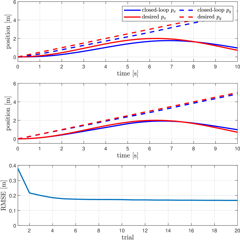
Figure 1: DiffTune for NMPC with a unicycle model. The top and middle rows show the tracking performance of the closed-loop system before and after using DiffTune, respectively. The bottom row shows the RMSE history over learning trials.

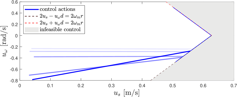
Figure 2: Optimal closed-loop control actions through the learning trials. The lightest and darkest blue curves stand for trials 1 and 20, respectively.

We first apply DiffTune to learn an NMPC with the following nonlinear unicycle model:

$$\dot{p}_{x}=\cos(\theta)u_{s},\ \dot{p}_{y}=\sin(\theta)u_{s},\ \dot{\theta}=u_{\omega},$$ (8)

where the system state $\bm{x}=[p_{x},p_{y},\theta]^{\top}$ includes the horizontal position $p_{x}$, vertical position $p_{y}$, and heading angle $\theta$, and the control action $\bm{u}=[u_{s},u_{\omega}]^{\top}$ includes the speed $u_{s}$ and angular velocity $u_{\omega}$. The unicycle has a differential drive with two wheels (radius $r=0.1$ m) of distance $d=0.5$ m in between. The maximum angular velocity for each wheel is set to $\omega_{m}=2\pi$ rad/s. Considering the geometry and the angular velocity limit of each wheel above, we can define the following linear inequalities on the control action $\bm{u}$:

$$-2\omega_{m}r\leq 2u_{s}+u_{w}d\leq 2\omega_{m}r,$$ (9)

$$-2\omega_{m}r\leq 2u_{s}-u_{w}d\leq 2\omega_{m}r.$$ (10)

We command the following reference trajectory for tracking: $\bar{\bm{x}}_{t}=[1-\cos(0.5t),0.5t,\arctan(1/{\sin(0.5t)})]^{\top}$. The NMPC problem has a planning horizon of 0.5 s with 0.05 s sample time ($T=10$), and $Q$ and $R$ are initialized to be $I_{3}$ and $I_{2}$, respectively. A total horizon of $10$ s ($N=200$) is considered for the closed-loop system. We apply DiffTune for 20 trials with a learning rate set to $\alpha=0.01$. The simulation results are shown in Figs. 1 and 2. Figure 1 shows the comparison of tracking performance before and after learning, as well as the RMSE reduction through the trials. It can be observed that the tracking performance has improved with the RMSE reduced from 0.38 to 0.17 m. The RMSE remains unchanged towards the end because the diagonal elements of $Q$ and $R$ reach the boundary. The evolution of the closed-loop control actions is shown in Fig. 2. Learning mainly influences the control actions in the first half of the horizon in each trial, where one can see the gradually shifted control actions for faster rotation $u_{w}$. For the remaining time in the horizon, the control actions are constrained to stay on the boundary of the feasible set, indicating limited performance improvement owing to the physical limits of the system.

V-B Quadrotor

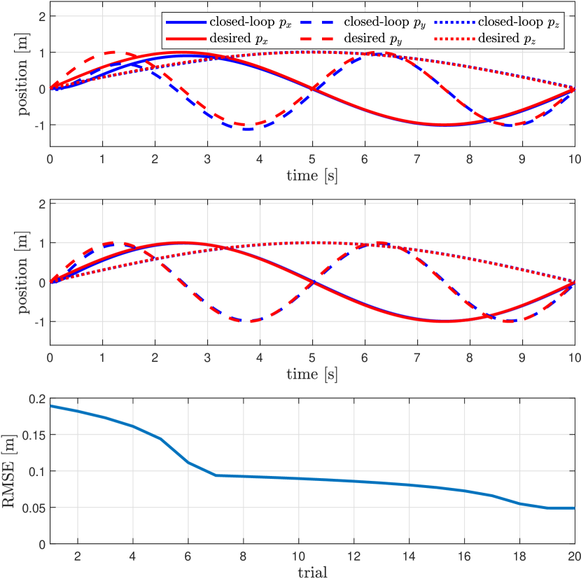
(a) 3D Figure 8 trajectory

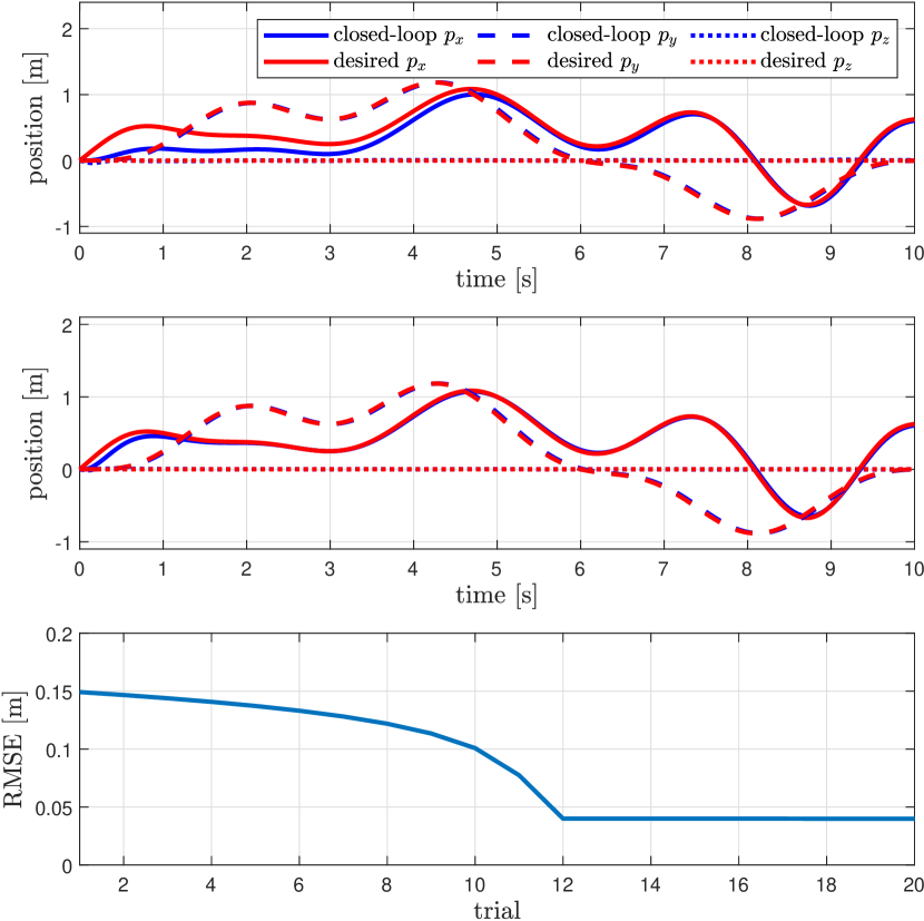
(b) Minimum-snap trajectory

Figure 3: Learning NMPC for quadrotor trajectory tracking on two trajectories. The top and middle rows show the tracking performance of the closed-loop system before and after using DiffTune. The bottom row shows the RMSE history over learning trials.

We apply DiffTune to learn an NMPC for quadrotor trajectory tracking. The nonlinear 6 DoF rigid body dynamics are given as follows:

$$\dot{\bm{p}}= \bm{v},\ \dot{\bm{v}}=m^{-1}f\bm{z}_{B}+\bm{g},$$ (11)

$$\dot{\bm{q}}= \frac{1}{2}\bm{q}\otimes[0\ \bm{\omega}^{\top}]^{\top},\ \dot{\bm{\omega}}=J^{-1}(\bm{M}-\bm{\omega}\times J\bm{\omega}),$$ (12)

where the state $\bm{x}=[{\bm{p}}^{\top}\ {\bm{v}}^{\top}\ {\bm{q}}^{\top}\ {\bm{\omega}}^{\top}]^{\top}$ and $\bm{p}=[p_{x},p_{y},p_{z}]^{\top}\in\mathbb{R}^{3}$, $\bm{v}\in\mathbb{R}^{3}$ denote the position and velocity of the quadrotor, both represented in the inertial frame, $\bm{q}\in\mathbb{S}^{3}$ is the quaternion representing the rotation from the inertial frame to the body frame (with $\otimes$ denoting the quaternion product), and $\bm{\omega}\in\mathbb{R}^{3}$ represents the angular velocity in body frame. The gravitational acceleration is denoted by $\bm{g}=[0\ 0\ -g]^{\top}$ (we use the ENU coordinate for both the body and inertial frame). The vector $\bm{z}_{B}$ is the unit vector aligning with the $z$-axis of the body frame, represented in the inertial frame. The control $\bm{u}$ contains four individual rotor thrusts and thus determines the total thrust ${f_{T}}$ and moment $\bm{M}\in\mathbb{R}^{3}$. The quadrotor has parameters $m=0.03$ kg and $J=10^{-5}\text{diag}(1.43,1.43,2.89)$ kgm².

Here, we command two reference trajectories: one is a 3D figure 8 trajectory, and the other one is a polynomial trajectory generated using minimum-snap optimization [24]. For both trajectories, the NMPC problem has a planning horizon of 0.5 s with 0.05 s sample time ($T=10$), and $Q$ and $R$ are initialized to be $I_{13}$ and $I_{4}$, respectively. A total horizon of $10$ s ($N=200$) is considered for the closed-loop system. We apply DiffTune for 20 trials with a learning rate set to $\alpha=0.05$. The simulation results are shown in Fig. 3. It can be observed that DiffTune can efficiently improve the tracking performance on these two trajectories by learning 17 parameters simultaneously.

Note that for the RMSE plot in Fig. 3(a), there are two sudden slope changes at trial 7 and trial 19. This is because at trial 7, one parameter in $Q$ reaches the minimum value of 0.01, and at trial 19, another parameter in $Q$ reaches the minimum value, and these two parameters affect the tracking performance the most. Thus, the RMSE cannot be further decreased and stays at the same value after trial 19. Similarly, for RMSE in Fig. 3(b), the key parameter affecting the tracking performance reaches the minimum value at trial 12, and thus the RMSE has stayed constant since then.

V-C Double Integrator

We use a simple linear system to illustrate the impact of control saturation on learning. Consider a 1D double-integrator system with friction

$$\dot{\bm{x}}(t)=\begin{bmatrix}\dot{p}(t)\\ \dot{v}(t)\end{bmatrix}=\begin{bmatrix}0&1\\ 0&-0.05\end{bmatrix}\bm{x}(t)+\begin{bmatrix}0\\ 1\end{bmatrix}u(t).$$ (13)

We command the following reference trajectory for tracking $\bar{\bm{x}}(t)=[1+t-\cos(t),\ 1+\sin(t)]^{\top}$. We consider the boxed constraint $|u|\leq u_{bd}$ for control constraints. We choose $u_{bd}=1,2,4$ to reflect the different magnitudes of constrained control actions. A total horizon of 10 s is considered with time intervals of 0.01 s for discretization. The planning horizon of MPC is 0.2 s ($T=20$). We apply DiffTune to these three cases for 20 trials each with the loss function set to the accumulated tracking error squared and learning rate $\alpha=0.1$. The optimal closed-loop control actions in the last trial are shown in Fig. 4(a), where the saturation at the beginning lasts for a shorter period for a bigger value of $u_{bd}$. Correspondingly, the tracking error has a larger reduction for larger values of $u_{bd}$ as shown in Fig. 4(b). This observation validates our earlier analysis in Section IV-A, where active constraints (saturated control) cap performance improvement by learning. Tighter constraints imply more frequent control saturation, which impedes the auto-tuning to improve tracking performance because saturation is a physical limitation that is beyond what learning is for.

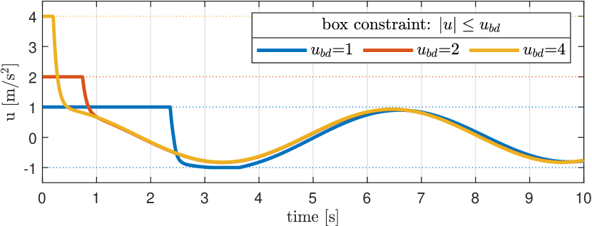
(a) Closed-loop optimal control in the final trial. Dashed lines indicate the boundary $u_{bd}$ of control actions.

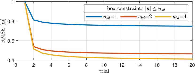
(b) RMSE reduction

Figure 4: Optimal control actions and RMSE reduction subject to box constraints with different levels of tightness $u_{bd}$. Tighter constraints imply more frequent control saturation, which impedes the learning from improving tracking performance.

V-D Comparison with Open-loop Learning [2]

We compare the tracking performance of a closed-loop system using an MPC with parameters trained in closed-loop by DiffTune-MPC and in open-loop by [2]. We use the same 1D double-integrator system (13) as the one used in Section V-C without control constraints. The learning goal for MPC is to track a reference trajectory $\bar{\bm{x}}(t)=[1+t-\cos(t),\ 1+\sin(t)]^{\top}$ for 10 s. The planning horizon of MPC is 1s. According to the open-loop nature of [2], the horizon of loss must be shorter than or equal to MPC’s horizon in open-loop learning. Thus, we define the horizons of the RMSE loss for the open-loop and closed-loop learning to be 1 s ($N=100$) and 10 s ($N=1000$), respectively. Nevertheless, we use RMSE as the loss function to average out the tracking errors on intervals with different lengths. Specifically, RMSE$=(\frac{1}{N}\sum_{i=1}^{N}(p_{i}-\bar{p}_{i})^{2})^{1/2}$ for $N$ being the horizon of the open-loop learning loss or closed-loop learning loss. Furthermore, we strive for a fair comparison by setting the same learning rate $\alpha=0.1$ and 20 trials for each learning scheme. Subsequently, the learned parameters are used in an MPC controller to track the same trajectory in a closed-loop manner for 10 s. The tracking error (measured by RMSE over the entire 10 s trajectory) of the parameters learned by DiffTune is 0.019 m, which is 12.5x smaller than the error 0.239 m with the open-loop method [2].

VI Conclusion

In this paper, we develop a closed-loop learning scheme for MPC using DiffTune. We learn the parameters in the cost function to improve the closed-loop system’s performance specified by a loss function that is different than the MPC’s cost function. To use DiffTune, we need the gradient of the first optimal control action with respect to the initial state and parameters of the cost function in the MPC problem. Our derivation is centered on a linear MPC problem with linear inequality constraints (to incorporate safety requirements of physical limitations of the system). We show that the linear-MPC-based differentiation can be applied to a nonlinear MPC that is solved via SQP. We validate our approach in simulation for systems with linear and nonlinear dynamics. We also show the limited performance improvement by learning when a system experiences control saturation both in analysis and by simulation. Lastly, we show the benefit of using DiffTune to learn the MPC cost function’s parameters for a better closed-loop performance than open-loop learning. Future work will investigate the usage of DiffTune for learning subject to multiple trajectories or tasks for improved generalization of the learned parameters.

Appendix

We show how the auxiliary problem (LMPC-Grad) is derived using the KKT condition in the Appendix. We start with an LQR and then cover the case with a general linear MPC (an LQR with linear inequality constraints).

VI-A Differentiation of an LQR

We start the illustration of obtaining the gradient of an LQR’s first optimal control action to the parameters of interest (cost coefficients and initial state). Consider the following LQR problem, where we stick to the same notation as in [2]:

$$\underset{\bm{\tau}_{1:T}}{\text{minimize}} \sum_{t=1}^{T}\frac{1}{2}\bm{\tau}_{t}^{\top}C_{t}\bm{\tau}_{t}+\bm{c}_{t}^{\top}\bm{\tau}_{t}$$

subject to $$\bm{x}_{t+1}=F_{t}\bm{\tau}_{t}+\bm{f}_{t},\ \bm{x}_{1}=\bm{x}_{\text{init}},$$ (P1)

where $\bm{\tau}_{t}=[\begin{smallmatrix}\bm{x}_{t}\\ \bm{u}_{t}\end{smallmatrix}]\in\mathbb{R}^{n+m}$ is the composite state-control, $F_{t}=[\begin{smallmatrix}A_{t}&B_{t}\end{smallmatrix}]\in\mathbb{R}^{n\times(n+m)}$, and $\bm{f}_{t}\in\mathbb{R}^{n}$ stands for residuals in the dynamics. With the Lagrangian

$$\mathcal{L}(\bm{\tau},\bm{\lambda}) =\sum_{t=1}^{T}\left(\frac{1}{2}\bm{\tau}^{\top}C_{t}\bm{\tau}_{t}+\bm{c}_{t}^{\top}\bm{\tau}_{t}\right)$$

$$+\sum_{t=0}^{T-1}\bm{\lambda}_{t}^{\top}(F_{t}\bm{\tau}_{t}+\bm{f}_{t}-\bm{x}_{t+1}),$$ (14)

where $\bm{\lambda}_{t}\in\mathbb{R}^{n}$ is the vector of the Lagrangian multipliers associated with the dynamics constraints, and $F_{0}=0$ and $\bm{f}_{0}=\bm{x}_{\text{init}}$ in the Lagrangian above. The solution to the LQR problem is obtained at the fixed point of the Lagrangian, i.e., when

$$\nabla_{\bm{\tau}_{t}}\mathcal{L}(\bm{\tau}^{\star},\bm{\lambda}^{\star})=C_{t}\bm{\tau}_{t}^{\star}+\bm{c}_{t}+F_{t}^{\top}\bm{\lambda}_{t}^{\star}-\begin{bmatrix}\bm{\lambda}^{\star}_{t-1}\\ 0\end{bmatrix}=0.$$ (15)

Following this relation, we can derive the costate dynamics

$$\bm{\lambda}_{T-1}^{\star}= C_{T,\bm{x}}\bm{x}_{T}^{\star}+\bm{c}_{T,\bm{x}},$$ (16)

$$\bm{\lambda}_{t}^{\star}= F_{t+1,\bm{x}}^{\top}\bm{\lambda}_{t+1}+C_{t+1,\bm{x}}\bm{x}_{t+1}^{\star}+\bm{c}_{t+1,\bm{x}},$$ (17)

for $t\in\{0,1,\dots,T-2\}$. The notation $C_{\cdot,\bm{x}}$, $F_{\cdot,\bm{x}}$, and $\bm{c}_{\cdot,\bm{x}}$ stands for the first $n$ columns of $C_{\cdot}$ and $F_{\cdot}$, and first $n$ rows of $\bm{c}_{\cdot}$, respectively. The original dynamics, costate dynamics, and the initial state allow for writing the KKT factorization in (18), where $K$ is the KKT factorization matrix.

$$\underbrace{\begin{bmatrix}\begin{array}[]{cc|cc|c|cc}&-[\begin{smallmatrix}I&0\end{smallmatrix}]&&&&&\\ -[\begin{smallmatrix}I\\ 0\end{smallmatrix}]&C_{1}&F_{1}^{\top}&&&&\\ &F_{1}&&-[\begin{smallmatrix}I&0\end{smallmatrix}]&&&\\ &&-[\begin{smallmatrix}I\\ 0\end{smallmatrix}]&C_{2}&&&\\ &&&&\ddots&&\\ &&&&&F_{T-1}^{\top}&\\ &&&&&&-[\begin{smallmatrix}I&0\end{smallmatrix}]\\ &&&&&-[\begin{smallmatrix}I\\ 0\end{smallmatrix}]&C_{T}\end{array}\end{bmatrix}}_{:=K}\left[\begin{array}[]{c}\bm{\lambda}_{0}^{\star}\\ \bm{\tau}_{1}^{\star}\\ \hline\cr\bm{\lambda}_{1}^{\star}\\ \bm{\tau}_{2}^{\star}\\ \hline\cr\vdots\\ \hline\cr\bm{\lambda}_{T-1}^{\star}\\ \bm{\tau}_{T}^{\star}\end{array}\right]=\begin{bmatrix}-\bm{x}_{\text{init}}\\ -\bm{c}_{1}\\ -\bm{f}_{1}\\ -\bm{c}_{2}\\ \vdots\\ -\bm{c}_{T-1}\\ -\bm{f}_{T-1}\\ -\bm{c}_{T}.\end{bmatrix}$$ (18)

To obtain the derivatives $\partial\bm{u}_{1}^{\star}/\partial\underline{C}_{t}$ and $\partial\bm{u}_{1}^{\star}/\partial\bm{c}_{t}$, we will take a look at the matrix differential of original dynamics, costate dynamics, and boundary conditions:

$$\text{d}\bm{x}_{t+1}= \text{d}F_{t}\bm{x}_{t}+F_{t}\text{d}\bm{x}_{t}+\text{d}\bm{f}_{t},$$ (19a)

$$\text{d}\bm{\lambda}_{t}^{\star}= \text{d}F_{t+1,\bm{x}}^{\top}\bm{\lambda}_{t+1}+F_{t+1,\bm{x}}^{\top}\text{d}\bm{\lambda}_{t+1}+\text{d}C_{t+1,\bm{x}}\bm{\tau}_{t+1}^{\star}$$

$$+C_{t+1,\bm{x}}\text{d}\bm{\tau}_{t+1}^{\star}+\text{d}\bm{c}_{t+1,\bm{x}},$$ (19b)

$$\text{d}\bm{x}_{1}= \text{d}\bm{x}_{\text{init}},$$ (19c)

$$\text{d}\bm{\lambda}_{T-1}^{\star}= \text{d}C_{T,\bm{x}}\bm{x}_{T}^{\star}+C_{T,\bm{x}}\text{d}\bm{x}_{T}^{\star}+\text{d}\bm{c}_{T,\bm{x}}.$$ (19d)

The KKT factorization for (19) can be presented as follows:

$$K\begin{bmatrix}\text{d}\bm{\lambda}_{0}^{\star}\\ \text{d}\bm{\tau}_{1}^{\star}\\ \text{d}\bm{\lambda}_{1}^{\star}\\ \text{d}\bm{\tau}_{2}^{\star}\\ \vdots\\ \text{d}\bm{\lambda}_{T-1}^{\star}\\ \text{d}\bm{\tau}_{T}^{\star}\end{bmatrix}=\begin{bmatrix}-\text{d}\bm{x}_{\text{init}}\\ -\text{d}\bm{c}_{1}-\text{d}C_{1}\bm{\tau}_{1}^{\star}-\text{d}F_{1}^{\top}\bm{\lambda}_{1}^{\star}\\ -\text{d}\bm{f}_{1}-\text{d}F_{1}\bm{\tau}_{1}^{\star}\\ -\text{d}\bm{c}_{2}-\text{d}C_{2}\bm{\tau}_{2}^{\star}-\text{d}F_{2}^{\top}\bm{\lambda}_{2}^{\star}\\ \vdots\\ -\text{d}\bm{c}_{T-1}-\text{d}C_{T-1}\bm{\tau}_{T-1}^{\star}-\text{d}F_{T-1}^{\top}\bm{\lambda}_{T-1}^{\star}\\ -\text{d}\bm{f}_{T-1}-\text{d}F_{T-1}\bm{\tau}_{T-1}^{\star}\\ -\text{d}\bm{c}_{T}-\text{d}C_{T}\bm{\tau}_{T}^{\star}\end{bmatrix}.$$ (20)

We start with the Jacobian $\partial\bm{u}_{1}^{\star}/\partial\bm{x}_{\text{init}}$ because it is simpler than the other two Jacobians. We set the differentials $\text{d}C_{t}$, $\text{d}\bm{c}_{t}$, $\text{d}F_{t}$, and $\text{d}\bm{f}_{t}$ to zero for $t\in\{1,2,\dots,T\}$ in (20) and we have

$$K\begin{bmatrix}\frac{\partial\bm{\lambda}_{0}^{\star}}{\partial\bm{x}_{\text{init}}}\\ \frac{\partial\bm{\tau}_{1}^{\star}}{\partial\bm{x}_{\text{init}}}\\ \vdots\\ \frac{\partial\bm{\lambda}_{T-1}^{\star}}{\partial\bm{x}_{\text{init}}}\\ \frac{\partial\bm{\tau}_{T}^{\star}}{\partial\bm{x}_{\text{init}}}\end{bmatrix}=\begin{bmatrix}-I_{n}\\ 0\\ \vdots\\ 0\\ 0\end{bmatrix},$$ (21)

where the target Jacobian $\partial\bm{u}_{1}^{\star}/\partial\bm{x}_{\text{init}}$ is contained within $\partial\bm{\tau}_{1}^{\star}/\partial\bm{x}_{\text{init}}$ such that

$$\frac{\partial\bm{\tau}_{1}^{\star}}{\partial\bm{x}_{\text{init}}}=\begin{bmatrix}\frac{\partial\bm{x}_{1}^{\star}}{\partial\bm{x}_{\text{init}}}\\ \frac{\partial\bm{u}_{1}^{\star}}{\partial\bm{x}_{\text{init}}}\end{bmatrix}.$$ (22)

If we compare the form and match the terms of (21) to the KKT factorization of the original problem in (18), then we can obtain $\partial\bm{u}_{1}^{\star}/\partial\bm{x}_{\text{init}}$ by solving the following auxiliary LQR problem

$$\underset{\tilde{\bm{\tau}}_{1:T}}{\text{minimize}} \sum_{t=1}^{T}\frac{1}{2}\tilde{\bm{\tau}}_{t}^{\top}\tilde{C}_{t}\tilde{\bm{\tau}}_{t}+\tilde{\bm{c}}_{t}^{\top}\tilde{\bm{\tau}}_{t}$$

subject to $$\tilde{\bm{x}}_{t+1}=\tilde{F}_{t}\tilde{\bm{\tau}}_{t}+\tilde{\bm{f}}_{t},\ \tilde{\bm{x}}_{1}=\tilde{\bm{x}}_{\text{init}}.$$ (LQR-Aux)

The gradient $\partial\bm{u}_{1}^{\star}/\partial[\bm{x}_{\text{init}}]_{j}$ can be solved from (VI-A) following the observations below. By (21), we have

$$K\begin{bmatrix}\frac{\partial\bm{\lambda}_{0}^{\star}}{\partial[\bm{x}_{\text{init}}]_{j}}\\ \frac{\partial\bm{\tau}_{1}^{\star}}{\partial[\bm{x}_{\text{init}}]_{j}}\\ \vdots\\ \frac{\partial\bm{\lambda}_{T-1}^{\star}}{\partial[\bm{x}_{\text{init}}]_{j}}\\ \frac{\partial\bm{\tau}_{T}^{\star}}{\partial[\bm{x}_{\text{init}}]_{j}}\end{bmatrix}=\begin{bmatrix}-I_{n}\\ 0\\ \vdots\\ 0\\ 0\end{bmatrix}_{:,j}.$$ (23)

Matching (23) with (18), $\partial\bm{u}_{1}^{\star}/\partial[\bm{x}_{\text{init}}]_{j}$ can be solved via (VI-A) with $\tilde{C}_{t}=C_{t}$, $\tilde{\bm{c}}_{t}=0$, $\tilde{F}_{t}=F_{t}$ , $\tilde{\bm{f}}_{t}=0$, and $\tilde{\bm{x}}_{\text{init}}=[I_{n}]_{:,j}=\bm{e}_{j}^{n}$.

Similarly, for the Jacobian $\partial\bm{u}_{1}^{\star}/\partial\underline{C}_{t}$, we start with

$$\text{d}C_{t}\bm{\tau}_{t}^{\star}=((\bm{\tau}_{t}^{\star})^{\top}\otimes I_{n+m})\text{d}\underline{C}_{t}$$ (24)

using the vectorization (with Kronecker product) formula $\underline{ABC}=(C^{\top}\otimes A)\underline{B}$. This equation will lead to the factorization

$$K\begin{bmatrix}*\\ \partial\bm{\tau}_{1}^{\star}/\partial\underline{C}_{t}\\ *\end{bmatrix}=\begin{bmatrix}0\\ \vdots\\ \begin{bmatrix}-(\bm{\tau}_{t}^{\star})^{\top}\otimes I_{n+m}\end{bmatrix}\\ 0\\ \vdots\end{bmatrix}.$$ (25)

Matching (25) with (18), given any specific $t$, the derivative $\partial\bm{u}_{1}^{\star}/\partial[C_{t}]_{i,j}$ can be solved from (VI-A) with $\tilde{C}_{t}=C_{t}$, $\tilde{F}_{t}=F_{t}$, $\tilde{\bm{f}}_{t}=0$ for all $t$, $\tilde{\bm{x}}_{\text{init}}=0$, and $\tilde{\bm{c}}_{t}=[(\bm{\tau}_{t}^{\star})^{\top}\otimes I_{n+m}]_{:,(i-1)(n+m)+j}=[\bm{\tau}_{t}^{\star}]_{j}\bm{e}_{i}^{n+m}$ for this specific $t$ and $\tilde{\bm{c}}_{t^{\prime}}=0$ for all $t^{\prime}\neq t$. Likewise, if one wants to get $\partial\bm{u}_{1}^{\star}/\partial[\bm{c}_{t}]_{i}$, then it suffices to solve (VI-A) with $\tilde{\bm{c}}_{t}=\bm{e}^{n+m}_{i}$ and $\tilde{\bm{c}}_{t^{\prime}}=0$ for all $t^{\prime}\neq t$.

VI-B Differentiation of an LQR with $(Q,R)$-parametrization

In this case, we use the $(Q,R)$-parameterization with coefficients of the $Q_{t}\in\mathbb{R}^{n\times n}$ and $R_{t}\in\mathbb{R}^{m\times m}$ matrices in the cost function, which are composited as $C_{t}=\text{diag}(Q_{t},R_{t})$ following the notation in (VI-A). Note that $\bm{c}_{t}$ also contains the coefficients of $Q_{t}$ and $R_{t}$ such that $\bm{c}_{t}=-[\begin{smallmatrix}Q_{t}&\\ &R_{t}\end{smallmatrix}]\bar{\bm{\tau}_{t}}$ for $\bar{\bm{\tau}}_{t}=[\begin{smallmatrix}\bar{\bm{x}}_{t}\\ \bar{\bm{u}}_{t}\end{smallmatrix}]$.

For $\partial\bm{u}_{1}^{\star}/\partial\underline{Q}_{t}$, one can apply the same methodology as applied in the previous subsection. Note that

$$\text{d}C_{t}\bm{\tau}_{t}^{\star}+\text{d}\bm{c}_{t}= \begin{bmatrix}\text{d}Q_{t}(\bm{x}_{t}^{\star}-\bar{\bm{x}}_{t})\\ \text{d}R_{t}(\bm{u}_{t}^{\star}-\bar{\bm{u}}_{t})\end{bmatrix}$$ (26)

$$= \begin{bmatrix}\left((\bm{x}_{t}^{\star}-\bar{\bm{x}}_{t})^{\top}\otimes I_{n}\right)\text{d}\underline{Q}_{t}\\ \left((\bm{u}_{t}^{\star}-\bar{\bm{u}}_{t})^{\top}\otimes I_{m}\right)\text{d}\underline{R}_{t}\end{bmatrix}$$ (27)

If $Q_{t}$ is symmetric, then $\text{d}Q_{t}(\bm{x}_{t}^{\star}-\bar{\bm{x}}_{t})=\dfrac{1}{2}\left((\bm{x}_{t}^{\star}-\bar{\bm{x}}_{t})^{\top}\otimes I_{n}+I_{n}\otimes(\bm{x}_{t}^{\star}-\bar{\bm{x}}_{t})^{\top}\right)\text{d}\underline{Q}_{t}$ (the same conclusion applies to a symmetric matrix $R_{t}$). Hence, we have

$$K\begin{bmatrix}*\\ \partial\bm{\tau}_{1}^{\star}/\partial[{Q}_{t}]_{i,j}\\ *\end{bmatrix}=\begin{bmatrix}0\\ \vdots\\ \begin{bmatrix}-(\bm{x}_{t}^{\star}-\bar{\bm{x}}_{t})^{\top}\otimes I_{n}\\ 0\end{bmatrix}\\ 0\\ \vdots\end{bmatrix}_{:,(i-1)n+j}.$$ (28)

In other words, the derivative $\partial\bm{u}_{1}^{\star}/\partial[Q_{t}]_{i,j}$ can be solved from (VI-A) with $\tilde{C}_{t}=C_{t}$, $\tilde{F}_{t}=F_{t}$, $\tilde{\bm{f}}_{t}=0$, $\tilde{\bm{x}}_{\text{init}}=0$ for all $t$, and $\tilde{\bm{c}}_{t}=\begin{bmatrix}(\bm{x}_{t}^{\star}-\bar{\bm{x}}_{t})^{\top}\otimes I_{n}\\ 0\end{bmatrix}_{:,(i-1)n+j}=\begin{bmatrix}[\bm{x}_{t}^{\star}-\bar{\bm{x}}_{t}]_{j}\bm{e}_{i}^{n}\\ 0\end{bmatrix}$ for this specific $t$ and $\tilde{\bm{c}}_{t^{\prime}}=0$ for all $t^{\prime}\neq t$. One can apply similar derivations to obtain $\partial\bm{u}_{1}^{\star}/\partial[R_{t}]_{i,j}$ from (VI-A) with $\tilde{\bm{x}}_{\text{init}}=0$ for all $t$, and $\tilde{\bm{c}}_{t}=\begin{bmatrix}0\\ (\bm{u}_{t}^{\star}-\bar{\bm{u}}_{t})^{\top}\otimes I_{n}\end{bmatrix}_{:,(i-1)n+j}=\begin{bmatrix}0\\ [\bm{u}_{t}^{\star}-\bar{\bm{u}}_{t}]_{j}\bm{e}_{i}^{m}\end{bmatrix}$ and $\tilde{\bm{c}}_{t^{\prime}}=0$ for all $t^{\prime}\neq t$.

VI-C Differentiation of an LQR with linear inequality constraints

A slightly enhanced version of LQR includes path constraints on the state and control, e.g., with linear inequalities, which results in the formulation of (LMPC). Following the derivation in Appendix A, we can write the Lagrangian for (LMPC) as

$$\mathcal{L}(\bm{\tau},\bm{\lambda},\bm{\nu})$$

$$= \sum_{t=1}^{T}\left(\frac{1}{2}\bm{\tau}_{t}^{\top}C_{t}\bm{\tau}_{t}+\bm{c}_{t}^{\top}\bm{\tau}_{t}\right)+\sum_{t=0}^{T-1}\bm{\lambda}_{t}^{\top}(F_{t}\bm{\tau}_{t}+\bm{f}_{t}-\bm{x}_{t+1})$$

$$+\sum_{t=1}^{T}\bm{\nu}_{t}^{\top}(G_{t}\bm{\tau}_{t}-\bm{l}_{t}),$$ (29)

where $\bm{\nu}_{t}\in\mathbb{R}^{g}$ is the Lagrange multiplier associated with the inequality constraints. Let $\mathcal{I}_{t,\text{act}}\subseteq\{1,2,\dots,g\}$ denote the rows where the inequality $G_{t}\bm{\tau}_{t}\leq\bm{l}_{t}$ is active, i.e., $[G_{t}]_{\mathcal{I}_{t,\text{act}}}\bm{\tau}_{t}=[\bm{l}_{t}]_{\mathcal{I}_{t,\text{act}}}$. Correspondingly, $\mathcal{I}_{t,\text{ina}}=\{1,2,\dots,g\}\setminus\mathcal{I}_{t,\text{act}}$ denotes the inactive constraints, i.e., $[G_{t}]_{\mathcal{I}_{t,\text{ina}}}\bm{\tau}_{t}<[\bm{l}_{t}]_{\mathcal{I}_{t,\text{ina}}}$ Following the complementary slackness [25], we know the following condition holds at the optimality point:

$$[\bm{\nu}_{t}]_{\mathcal{I}_{t,\text{ina}}}=0,\quad[G_{t}]_{\mathcal{I}_{t,\text{ina}}}\bm{\tau}_{t}-[\bm{l}_{t}]_{\mathcal{I}_{t,\text{ina}}}<0,$$ (30)

$$[G_{t}]_{\mathcal{I}_{t,\text{act}}}\bm{\tau}_{t}-[\bm{l}_{t}]_{\mathcal{I}_{t,\text{act}}}=0,\quad[\bm{\nu}_{t}]_{\mathcal{I}_{t,\text{act}}}>0.$$ (31)

The costate dynamics for (LMPC) are

$$\bm{\lambda}_{T-1}^{\star}= C_{T,\bm{x}}\bm{x}_{T}^{\star}+\bm{c}_{T,\bm{x}}+G_{T,\bm{x}}^{\top}\bm{\nu}_{T}^{\star},$$ (32)

$$\bm{\lambda}_{t}^{\star}= F_{t+1,\bm{x}}^{\top}\bm{\lambda}_{t+1}+C_{t+1,\bm{x}}\bm{x}_{t+1}^{\star}+\bm{c}_{t+1,\bm{x}}+G_{t,\bm{x}}^{\top}\bm{\nu}_{t}^{\star}.$$ (33)

We can write down the KKT factorization for (LMPC) as shown in (34), with the KKT factorization matrix denoted by $K_{LI}$.

$$\underbrace{\begin{bmatrix}\begin{array}[]{ccc|ccc|c|ccc}&-[\begin{smallmatrix}I&0\end{smallmatrix}]&&&&&&&&\\ -[\begin{smallmatrix}I\\ 0\end{smallmatrix}]&C_{1}&G_{1}^{\top}&F_{1}^{\top}&&&&&&\\ &&I_{\mathcal{I}_{1,\text{ina}}}&&&&&&&\\ &[G_{1}]_{\mathcal{I}_{1,\text{act}}}&&&&&&&&\\ &F_{1}&&&-[\begin{smallmatrix}I&0\end{smallmatrix}]&&&&&\\ &&&-[\begin{smallmatrix}I\\ 0\end{smallmatrix}]&C_{2}&G_{2}^{\top}&&&\\ &&&&&I_{\mathcal{I}_{2,\text{ina}}}&&&&\\ &&&&[G_{2}]_{\mathcal{I}_{2,\text{act}}}&&&&&\\ &&&&&&\ddots&&&\\ &&&&&&&&-[\begin{smallmatrix}I&0\end{smallmatrix}]&\\ &&&&&&&-[\begin{smallmatrix}I\\ 0\end{smallmatrix}]&C_{T}&G_{T}^{\top}\\ &&&&&&&&&I_{\mathcal{I}_{T,\text{ina}}}\\ &&&&&&&&[G_{T}]_{\mathcal{I}_{T,\text{act}}}&\\ \end{array}\end{bmatrix}}_{:=K_{LI}}\left[\begin{array}[]{c}\bm{\lambda}_{0}^{\star}\\ \bm{\tau}_{1}^{\star}\\ \bm{\nu}_{1}^{\star}\\ \hline\cr\bm{\lambda}_{1}^{\star}\\ \bm{\tau}_{2}^{\star}\\ \bm{\nu}_{2}^{\star}\\ \hline\cr\vdots\\ \hline\cr\bm{\lambda}_{T-1}^{\star}\\ \bm{\tau}_{T}^{\star}\\ \bm{\nu}_{t}^{\star}\end{array}\right]=\begin{bmatrix}-\bm{x}_{\text{init}}\\ -\bm{c}_{1}\\ 0_{\mathcal{I}_{1,\text{ina}}}\\ [\bm{l}_{1}]_{\mathcal{I}_{1,\text{act}}}\\ -\bm{f}_{1}\\ -\bm{c}_{2}\\ 0_{\mathcal{I}_{2,\text{ina}}}\\ [\bm{l}_{2}]_{\mathcal{I}_{1,\text{act}}}\\ \vdots\\ -\bm{f}_{T-1}\\ -\bm{c}_{T}\\ 0_{\mathcal{I}_{T,\text{ina}}}\\ [\bm{l}_{t}]_{\mathcal{I}_{T,\text{act}}}.\end{bmatrix}$$ (34)

For the differentials associated with (LMPC), we have

$$K_{LI}\begin{bmatrix}\text{d}\bm{\lambda}_{0}^{\star}\\ \text{d}\bm{\tau}_{1}^{\star}\\ \text{d}\bm{\nu}_{1}^{\star}\\ \vdots\\ \text{d}\bm{\lambda}_{T-1}^{\star}\\ \text{d}\bm{\tau}_{T}^{\star}\\ \text{d}\bm{\nu}_{T}^{\star}\end{bmatrix}=\begin{bmatrix}-\text{d}\bm{x}_{\text{init}}\\ -\text{d}\bm{c}_{1}-\text{d}C_{1}\bm{\tau}_{1}^{\star}-\text{d}F_{1}^{\top}\bm{\lambda}_{1}^{\star}-\text{d}G_{1}^{\top}\bm{\nu}_{1}^{\star}\\ 0_{\mathcal{I}_{1,\text{ina}}}\\ -\text{d}[G_{1}]_{\mathcal{I}_{1,\text{act}}}\bm{\tau}_{1}^{\star}+\text{d}[\bm{l}_{1}]_{\mathcal{I}_{1,\text{act}}}\\ \vdots\\ -\text{d}\bm{f}_{T-1}-\text{d}F_{T-1}\bm{\tau}_{T-1}^{\star}\\ -\text{d}\bm{c}_{T}-\text{d}C_{T}\bm{\tau}_{T}^{\star}-\text{d}G_{T}^{\top}\bm{\nu}_{T}^{\star}\\ 0_{\mathcal{I}_{1,\text{ina}}}\\ -\text{d}[G_{T}]_{\mathcal{I}_{T,\text{act}}}\bm{\tau}_{1}^{\star}+\text{d}[\bm{l}_{t}]_{\mathcal{I}_{T,\text{act}}}\end{bmatrix}$$ (35)

One observation follows from (35): when considering the Jacobians with respect to $C_{t}$ and $\bm{c}_{t}$, then only non-zero differentials on the right-hand side of (35) will be $\text{d}C_{t}$ and $\text{d}\bm{c}_{t}$, which resembles the structure of the right-hand side of (20). This observation indicates that the gradients $\partial\bm{u}_{1}^{\star}/\partial\underline{C}_{t}$ and $\partial\bm{u}_{1}^{\star}/\partial\bm{c}_{t}$ can be obtained following the approach shown before with LQR in Appendix A.

Following the derivation in Appdendix A for (VI-A), one can solve the following auxiliary problem to obtain the gradient for (LMPC):

$$\underset{\tilde{\bm{\tau}}_{1:T}}{\text{minimize}} \sum_{t=1}^{T}\frac{1}{2}\tilde{\bm{\tau}}_{t}^{\top}\tilde{C}_{t}\tilde{\bm{\tau}}_{t}+\tilde{\bm{c}}_{t}^{\top}\tilde{\bm{\tau}}_{t}$$

subject to $$\tilde{\bm{x}}_{t+1}=\tilde{F}_{t}\tilde{\bm{\tau}}_{t}+\tilde{\bm{f}}_{t},\ \tilde{\bm{x}}_{1}=\tilde{\bm{x}}_{\text{init}},$$

$$\tilde{G}_{t}\tilde{\bm{\tau}}_{t}=\tilde{\bm{l}}_{t}.$$ (LMPC-Aux)

Specifically, to obtain the gradient $\partial\bm{u}_{1}^{\star}/\partial[C_{t}]_{i,j}$, one only needs to solve (LMPC-Aux) with $\tilde{C}_{t}=C_{t}$, $\tilde{\bm{c}}_{t}=\begin{bmatrix}(\bm{\tau}_{1}^{\star})^{\top}\otimes I_{n+m}\end{bmatrix}_{:,(i-1)(n+m)+j}=[\bm{\tau}_{t}^{\star}]_{j}\bm{e}_{i}^{n+m}$, $\tilde{\bm{f}}_{t}=0$, $\tilde{\bm{x}}_{\text{init}}=0$, $\tilde{G}_{t}=[G_{t}]_{\mathcal{I}_{t,\text{act}}}$, and $\tilde{\bm{l}}_{t}=0$. Likewise, to solve for the gradient $\partial\bm{u}_{1}^{\star}/\partial[\bm{c}_{t}]_{i}$, we can solve the problem (LMPC-Aux) with $\tilde{C}_{t}=C_{t}$, $\tilde{\bm{c}}_{t}=\bm{e}_{i}^{n+m}$, $\tilde{\bm{f}}_{t}=0$, $\tilde{\bm{x}}_{\text{init}}=0$, $\tilde{G}_{t}=[G_{t}]_{\mathcal{I}_{t,\text{act}}}$, and $\tilde{\bm{l}}_{t}=0$. To solve for $\partial\bm{u}_{1}^{\star}/\partial[\bm{x}_{\text{init}}]_{j}$, one can solve (LMPC-Aux) with $\tilde{C}_{t}=C_{t}$, $\tilde{\bm{c}}_{t}=0$, $\tilde{\bm{f}}_{t}=0$, $\tilde{\bm{x}}_{\text{init}}=\bm{e}_{j}^{n}$, $\tilde{G}_{t}=[G_{t}]_{\mathcal{I}_{t,\text{act}}}$, and $\tilde{\bm{l}}_{t}=0$. These results are summarized in (LMPC-Grad) and Table I in the text.

Note that the inequality constraints $G_{t}\bm{\tau}_{t}\leq\bm{l}_{t}$ in (LMPC) are turned into an equality constraint $\tilde{G}_{t}\tilde{\bm{\tau}}_{t}=\tilde{\bm{l}}_{t}$ in (LMPC-Aux), where the latter equality constraint only holds for those time indices $t$ with the constraint being active at the optimal solution $\bm{\tau}_{t}^{\star}$, i.e., $\tilde{G}_{t}=[G_{t}]_{\mathcal{I}_{t,\text{act}}}$. The inactive constraints (at the optimal solution of (LMPC)) are not considered in (LMPC-Aux) because the optimal solution of (LMPC) is “locally unconstrained” at the inactive constraints, i.e., removing the inactive constraints will not change the optimal solution. Therefore, the inactive constraints $[G_{t}]_{\mathcal{I}_{t,\text{ina}}}$ are not inherited from (LMPC) to (LMPC-Grad), and only active constraints show up in (LMPC-Grad) in the form of $\tilde{G}_{t}\tilde{\bm{\tau}}_{t}=0$ for $\tilde{G}_{t}=[G_{t}]_{\mathcal{I}_{t,\text{act}}}$.

References

- [1] S. Cheng, M. Kim, L. Song, Z. Wu, S. Wang, and N. Hovakimyan, “Difftune: Auto-tuning through auto-differentiation,” under revision for IEEE Transactions on Robotics, arXiv preprint arXiv:2209.10021, 2023.
- [2] B. Amos, I. Jimenez, J. Sacks, B. Boots, and J. Z. Kolter, “Differentiable MPC for end-to-end planning and control,” in Proceedings of the 32nd Conference on Neural Information Processing Systems, vol. 31, Montreal, Canada, 2018.
- [3] W. Jin, S. Mou, and G. J. Pappas, “Safe Pontryagin differentiable programming,” Advances in Neural Information Processing Systems, vol. 34, pp. 16 034–16 050, 2021.
- [4] H. Parwana and D. Panagou, “Recursive feasibility guided optimal parameter adaptation of differential convex optimization policies for safety-critical systems,” arXiv:2109.10949, 2021.
- [5] S. Cheng, L. Song, M. Kim, S. Wang, and N. Hovakimyan, “Difftune+: Hyperparameter-free auto-tuning using auto-differentiation,” in Learning for Dynamics and Control Conference. PMLR, 2023, pp. 170–183.
- [6] A. R. Kumar and P. J. Ramadge, “DiffLoop: Tuning PID controllers by differentiating through the feedback loop,” in Proceedings of the 55th Annual Conference on Information Sciences and Systems, Baltimore, MD, USA, 2021, pp. 1–6.
- [7] F. Berkenkamp, A. P. Schoellig, and A. Krause, “Safe controller optimization for quadrotors with Gaussian processes,” in Proceedings of IEEE International Conference on Robotics and Automation, Stockholm, Sweden, 2016, pp. 491–496.
- [8] R. R. Duivenvoorden, F. Berkenkamp, N. Carion, A. Krause, and A. P. Schoellig, “Constrained Bayesian optimization with particle swarms for safe adaptive controller tuning,” IFAC-PapersOnLine, vol. 50, no. 1, pp. 11 800–11 807, 2017.
- [9] A. Loquercio, A. Saviolo, and D. Scaramuzza, “Autotune: Controller tuning for high-speed flight,” IEEE Robotics and Automation Letters, vol. 7, no. 2, pp. 4432–4439, 2022.
- [10] W. Edwards, G. Tang, G. Mamakoukas, T. Murphey, and K. Hauser, “Automatic tuning for data-driven model predictive control,” in Proceedings of the IEEE International Conference on Robotics and Automation, Xi’an, China, 2021, pp. 7379–7385.
- [11] W. D. Null, W. Edwards, D. Jeong, T. Tchalakov, J. Menezes, K. Hauser et al., “Automatically-tuned model predictive control for an underwater soft robot,” IEEE Robotics and Automation Letters, 2023.
- [12] W. Jin, Z. Wang, Z. Yang, and S. Mou, “Pontryagin differentiable programming: An end-to-end learning and control framework,” in Proceedings of the 34th Conference on Neural Information Processing Systems, vol. 33, Vancouver, Canada, 2020, pp. 7979–7992.
- [13] A. Oshin and E. A. Theodorou, “Differentiable robust model predictive control,” arXiv preprint arXiv:2308.08426, 2023.
- [14] M. Zanon and S. Gros, “Safe reinforcement learning using robust MPC,” IEEE Transactions on Automatic Control, vol. 66, no. 8, pp. 3638–3652, 2020.
- [15] A. Romero, Y. Song, and D. Scaramuzza, “Actor-critic model predictive control,” arXiv preprint arXiv:2306.09852, 2023.
- [16] G. Torrente, E. Kaufmann, P. Föhn, and D. Scaramuzza, “Data-driven mpc for quadrotors,” IEEE Robotics and Automation Letters, vol. 6, no. 2, pp. 3769–3776, 2021.
- [17] K. Y. Chee, T. Z. Jiahao, and M. A. Hsieh, “KNODE-MPC: A knowledge-based data-driven predictive control framework for aerial robots,” IEEE Robotics and Automation Letters, vol. 7, no. 2, pp. 2819–2826, 2022.
- [18] K. Y. Chee, T. C. Silva, M. A. Hsieh, and G. J. Pappas, “Enhancing sample efficiency and uncertainty compensation in learning-based model predictive control for aerial robots,” arXiv preprint arXiv:2308.00570, 2023.
- [19] T. Z. Jiahao, K. Y. Chee, and M. A. Hsieh, “Online dynamics learning for predictive control with an application to aerial robots,” in Conference on Robot Learning. PMLR, 2023, pp. 2251–2261.
- [20] A. Saviolo, G. Li, and G. Loianno, “Physics-inspired temporal learning of quadrotor dynamics for accurate model predictive trajectory tracking,” IEEE Robotics and Automation Letters, vol. 7, no. 4, pp. 10 256–10 263, 2022.
- [21] N. Parikh, S. Boyd et al., “Proximal algorithms,” Foundations and Trends® in Optimization, vol. 1, no. 3, pp. 127–239, 2014.
- [22] P. T. Boggs and J. W. Tolle, “Sequential quadratic programming,” Acta numerica, vol. 4, pp. 1–51, 1995.
- [23] R. Verschueren, G. Frison, D. Kouzoupis, J. Frey, N. van Duijkeren, A. Zanelli, B. Novoselnik, T. Albin, R. Quirynen, and M. Diehl, “acados – a modular open-source framework for fast embedded optimal control,” Mathematical Programming Computation, Oct 2021.
- [24] D. Mellinger and V. Kumar, “Minimum snap trajectory generation and control for quadrotors,” in Proceedings fo the International Conference on Robotics and Automation, Shanghai, China, 2011, pp. 2520–2525.
- [25] S. P. Boyd and L. Vandenberghe, Convex optimization. Cambridge university press, 2004.