Four state deterministic cellular automaton rule emulating random diffusion

Abstract

We show how to construct a deterministic nearest-neighbour cellular automaton (CA) with four states which emulates diffusion on a one-dimensional lattice. The pseudo-random numbers needed for directing random walkers in the diffusion process are generated with the help of rule 30. This CA produces density profiles which agree very well with solutions of the diffusion equation, and we discuss this agreement for two different boundary and initial conditions. We also show how our construction can be generalized to higher dimensions.

1 Introduction

Modeling of diffusion processes with cellular automata (CA) is almost as old as the field of cellular automata itself. Lattice gas automata models [7] can simulate diffusion of real gas [4] very realistically and they were extensively studied in the last several decades, thus abundant literature of the subject exists, including monographs and textbooks [5, 11, 13, 16]. Various models of diffusion using lattice gases were investigated in recent years, for example [1, 9, 10]

Lattice gas automata are relatively complicated compared to “classical” CA. Even in the simplest HPP model [7] there are up to four particles per lattice site and each particle is characterized by one of the four allowed velocity vectors. Moreover, the update step consists of two substeps, movement of particles in the direction of the velocity vector followed by the collisions step when the directions of velocity vectors of some particles are changed. In more advanced models, such as, for example, reactive lattice gas automata [2, 15], there are three substeps, namely interaction, randomization and propagation. In the randomization substep the call to a pseudo-random generator is required for each lattice node.

In contrast to the above, in regular CA there are no velocity vectors attached to particles, and the update is done in a single time step with no need of substeps. The lattice sites change their state simultaneously at each time step according to a specified local rule which is purely deterministic, thus there is no need to call a random number generator.

We argue that for some applications it would be advantageous to have such a simple deterministic nearest-neighbour cellular automaton mimicking diffusion process, so that it could be used as a building block for various “complexity engineering” tasks. For example, it could be used to constructs solutions of classification problems in which diffusive spreading of agents is required, like in recently proposed “diffusive” solution of density classification problem [6].

What we would like to discuss in this paper, therefore, is a model of diffusion which is not based on lattice gas automata but rather on “classical” cellular automata. It is a model of an assembly of random walkers which perform random walk on a lattice following exclusion principle, that is, one lattice site can be occupied by only one walker at a time.

2 Construction of the rule

Consider one dimensional lattice with lattice sites being either empty (state 0) or occupied by a single particle (state 1). All particles simultaneously and independently of each other decide whether to move to the left or to the right, with the same probability 0.5 in either direction. We then simultaneously move every particle to the desired position if it is empty, otherwise the particle stays in the same place. If two particles want to move to the same empty spot, only one of them, randomly selected, is allowed to do so. This process, which constitutes a single time step, is then repeated for as many time steps as desired.

In order to describe the process more formally, let us denote by $s_{i}$ the state of the lattice site $i$, and let $X_{i}$ denote binary random variable attached to site $i$. All variables $X_{i}$ should be independent and identically distributed such that $Pr\left(X_{i}=0\right)=Pr\left(X_{i}=1\right)=1/2$. We give the following interpretation to values of random variables $X_{i}$. If $s_{i}=1$, then $X_{i}=1$ ($X_{i}=0$) means that movement of the particle from site $i$ to the right (left) is allowed. If $s_{i}=0$, then $X_{i}=1$ ($X_{i}=0$) means that arrival from the right (left) of site $i$ is allowed. If movement or arrival is not allowed, the particle does not move. With this notation, the state of the site $i$ at the next time step, denoted by $s_{i}^{\prime}$, can be expressed as follows.

$$s_{i}^{\prime}=s_{i}-\underbrace{s_{i}X_{i}\left(1-s_{i+1}\right)\left(1-X_{i+1}\right)}_{move\,\,to\,\,the\,\,right}-\underbrace{s_{i}\left(1-X_{i}\right)\left(1-s_{i-1}\right)X_{i-1}}_{move\,\,to\,\,the\,\,left}$$

$$+\underbrace{\left(1-s_{i}\right)\left(1-X_{i}\right)s_{i-1}X_{i-1}}_{arrive\,\,from\,\,the\,\,left}+\underbrace{\left(1-s_{i}\right)X_{i}s_{i+1}\left(1-X_{i+1}\right)}_{arrive\,\,from\,\,the\,\,right}$$ (1)

The above equation can be simplified,

$$s_{i}^{\prime}=s_{i}+X_{i}X_{i-1}s_{i}-X_{i}X_{i-1}s_{i-1}+X_{i}X_{i+1}x_{i}-X_{i}X_{i+1}s_{i+1}$$

$$-X_{i}s_{i}+X_{i}s_{i+1}-X_{i-1}s_{i}+X_{i-1}s_{i-1}.$$ (2)

It is also easy to verify that for periodic boundary conditions on a lattice of length $L$,

$$\sum_{i=0}^{L-1}s_{i}^{\prime}=\sum_{i=0}^{L-1}s_{i},$$

meaning that the number of particles is conserved.

Eq. (2) represents a probabilistic cellular automaton, and if we had a way to simulate $X_{i}$ by some pseudo-random process, we could constructs a purely deterministic CA. This can be done by using elementary rule 30 [12, 17],

$$X_{i}^{\prime}=f_{30}(X_{i-1},X_{i},X_{i+1}),$$ (3)

where $f_{30}$ denotes local function of rule 30, which can be written as

$$f_{30}(x_{0},x_{1},x_{2})=(x_{0}+x_{1}+x_{2}+x_{1}x_{2})\mod 2.$$ (4)

This means that at each site $i$ we have two binary state variables, $s_{i}$ and $X_{i}$, evolving, respectively, according to eqs. (2) and (3). We can combine them together by introducing another variable,

$$y_{i}=2s_{i}+X_{i},$$

so that we obtain CA with four states, $y_{i}\in\{0,1,2,3\}$. This is a fully deterministic nearest neighbour CA given by

$$y_{i}^{\prime}=f(y_{i-1},y_{i},y_{i+1}),$$

where $f:\{0,1,2,3\}^{3}\rightarrow\{0,1,2,3\}$ is defined in the Table 1. Let us call $\{0,1\}$ lower states and $\{2,3\}$ upper states. Lower states represent empty sites, while upper states sites occupied by particles. Of course this mean that empty cell can be in two states (0 or 1) and a particle can be in two states as well (2 or 3). These “internal” states are used only for generation of random numbers.

Table 1: Rule table for the diffusive rule with four states. The entries represent $(y_{i-1},y_{i},y_{i+1})\rightarrow y_{i}^{\prime}$.

(0,0,0) $\rightarrow$ 0	(1,0,0) $\rightarrow$ 1	(2,0,0) $\rightarrow$ 0	(3,0,0) $\rightarrow$ 3
(0,0,1) $\rightarrow$ 1	(1,0,1) $\rightarrow$ 0	(2,0,1) $\rightarrow$ 1	(3,0,1) $\rightarrow$ 2
(0,0,2) $\rightarrow$ 0	(1,0,2) $\rightarrow$ 1	(2,0,2) $\rightarrow$ 0	(3,0,2) $\rightarrow$ 3
(0,0,3) $\rightarrow$ 1	(1,0,3) $\rightarrow$ 0	(2,0,3) $\rightarrow$ 1	(3,0,3) $\rightarrow$ 2
(0,1,0) $\rightarrow$ 1	(1,1,0) $\rightarrow$ 0	(2,1,0) $\rightarrow$ 1	(3,1,0) $\rightarrow$ 0
(0,1,1) $\rightarrow$ 1	(1,1,1) $\rightarrow$ 0	(2,1,1) $\rightarrow$ 1	(3,1,1) $\rightarrow$ 0
(0,1,2) $\rightarrow$ 3	(1,1,2) $\rightarrow$ 2	(2,1,2) $\rightarrow$ 3	(3,1,2) $\rightarrow$ 2
(0,1,3) $\rightarrow$ 1	(1,1,3) $\rightarrow$ 0	(2,1,3) $\rightarrow$ 1	(3,1,3) $\rightarrow$ 0
(0,2,0) $\rightarrow$ 2	(1,2,0) $\rightarrow$ 1	(2,2,0) $\rightarrow$ 2	(3,2,0) $\rightarrow$ 3
(0,2,1) $\rightarrow$ 3	(1,2,1) $\rightarrow$ 0	(2,2,1) $\rightarrow$ 3	(3,2,1) $\rightarrow$ 2
(0,2,2) $\rightarrow$ 2	(1,2,2) $\rightarrow$ 1	(2,2,2) $\rightarrow$ 2	(3,2,2) $\rightarrow$ 3
(0,2,3) $\rightarrow$ 3	(1,2,3) $\rightarrow$ 0	(2,2,3) $\rightarrow$ 3	(3,2,3) $\rightarrow$ 2
(0,3,0) $\rightarrow$ 1	(1,3,0) $\rightarrow$ 0	(2,3,0) $\rightarrow$ 1	(3,3,0) $\rightarrow$ 0
(0,3,1) $\rightarrow$ 3	(1,3,1) $\rightarrow$ 2	(2,3,1) $\rightarrow$ 3	(3,3,1) $\rightarrow$ 2
(0,3,2) $\rightarrow$ 3	(1,3,2) $\rightarrow$ 2	(2,3,2) $\rightarrow$ 3	(3,3,2) $\rightarrow$ 2
(0,3,3) $\rightarrow$ 3	(1,3,3) $\rightarrow$ 2	(2,3,3) $\rightarrow$ 3	(3,3,3) $\rightarrow$ 2

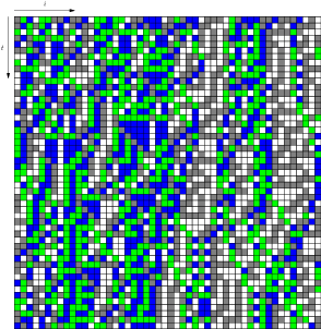
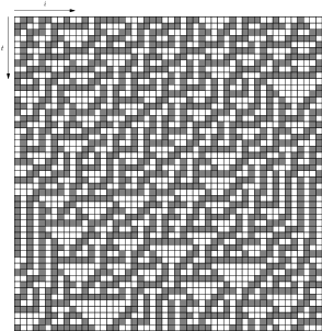
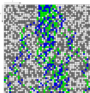
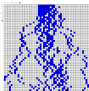
(a) (b)
(c) (d)

Figure 1: Spatiotemporal patterns for lattice with periodic boundary conditions and length $L=50$. (a) Random initial condition. (b) Random initial condition with only 0s and 1s. (c) Initial condition with block of 10 cells in upper states in the middle, lower states elsewhere; every 10th step is shown. (d) Identical pattern as in (c) but with lower states colored white and upper states blue.

Figure 1 shows examples of spatiotemporal patterns produced by this rule, with upper states shown in blue/green and lower states in grey/white. Random walk performed by individual particles is clearly visible. If we start with a lattice with all sites in lower states, the well known pattern produced by rule 30 can be observed (Fig. 1b).

We will now demonstrate that by taking the appropriate limit, eq. (2) actually leads to the partial differential equation known as diffusion or heat equation. Let $\rho_{i}=\langle s_{i}\rangle$, where the angle bracket denotes the expected value. Taking expected value of both sides of the eq. (2) we obtain

$$\rho_{i}^{\prime}=\rho_{i}+\frac{1}{4}\rho_{i}-\frac{1}{4}\rho_{i-1}+\frac{1}{4}\rho_{i}-\frac{1}{4}\rho_{i+1}-\frac{1}{2}\rho_{i}+\frac{1}{2}\rho_{i+1}-\frac{1}{2}\rho_{i}+\frac{1}{2}\rho_{i-1},$$ (5)

where we used the fact that $\langle X_{i}\rangle=1/2$ for all $i$. The above then simplifies to

$$\rho_{i}^{\prime}=\frac{1}{2}\rho_{i}+\frac{1}{4}\rho_{i+1}+\frac{1}{4}\rho_{i-1}.$$ (6)

We can write this as

$$\rho_{i}^{\prime}-\rho_{i}=\frac{1}{4}\left(\rho_{i+1}-2\rho_{i}+\frac{1}{4}\rho_{i-1}\right).$$ (7)

Let us now suppose that the system is updated in discrete time steps, where the time interval between updates is $\tau$. Moreover, let the spacing between lattice sites be $\epsilon$. If we divide both sides of the above equation by $\tau$ and multiply its right hand side by $\frac{\epsilon^{2}}{\epsilon^{2}}$ we obtain

$$\frac{\rho_{i}^{\prime}-\rho_{i}}{\tau}=\frac{\epsilon^{2}}{4\tau}\frac{\rho_{i+1}-2\rho_{i}+\rho_{i-1}}{\epsilon^{2}}.$$ (8)

It is now clear that the left hand side corresponds to numerical approximation of the first derivative of $\rho$ with respect to time, while the right hand side corresponds to the numerical approximation of the second derivative of $\rho$ with respect to the spatial coordinate. If we take the limit of both sides with $\epsilon\rightarrow 0$ and, at the same time, allowing $\tau$ tend to zero in such a way that $\epsilon^{2}/\tau$ remains constant, we get

$$\frac{\partial\rho}{\partial t}=D\frac{\partial^{2}\rho}{\partial x^{2}},$$ (9)

where $D=\epsilon^{2}/4\tau$, $x=i\epsilon$ represents spatial coordinate, and $t=k\tau$ represents time with $k$ denoting time step, $k\in\{0,1,2,\ldots\}$. This is indeed the diffusion equation. We will now show that orbits of our rule defined in Table 1 approximate solutions of eq. (9) remarkably well.

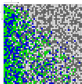
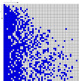
(a) (b)

Figure 2: (a) Spatiotemporal patterns for lattice with fixed boundary conditions and length $L=50$. Left end is the source of particles and the right end is kept empty. (a) Identical pattern as in (a) but with lower states colored white and upper states blue. Only every 10-th step is shown.

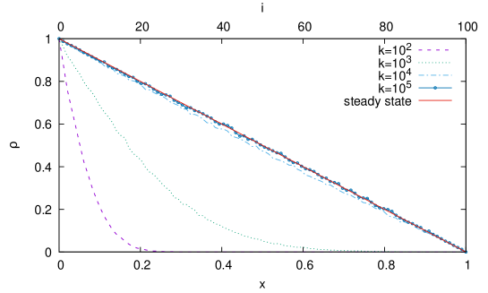
Figure 3: Density profiles obtained by numerical experiments for finite lattice ($L=100$) with inhomogeneous boundary conditions. Left end is the source of particles and the Right end is always empty. Vertical axis represents density obtained after $k$ iterations, averaged over $10^{4}$ runs.

(a)

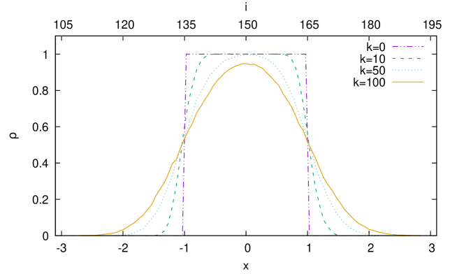
(b)

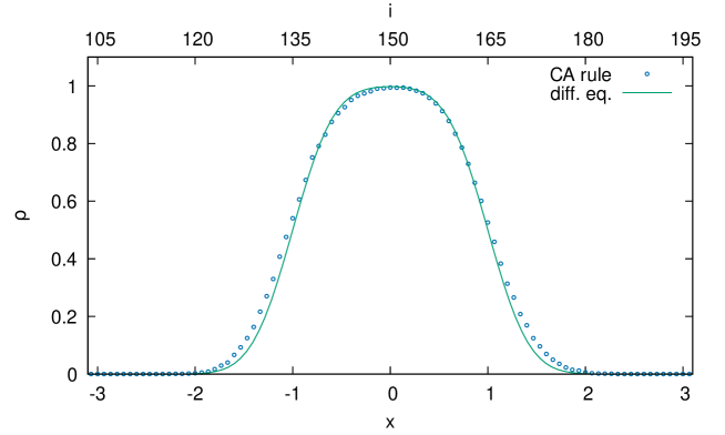
Figure 4: (a) Development of density profile for lattice of length $L=300$ with particles initially located only at $i=135,136,\ldots 165$. Vertical axis represents density obtained after $k$ iterations, averaged over $10^{4}$ runs. (b) Density profile for CA for $k=50$ compared with solution of the diffusion equation given by eq. (11).

3 Experiments

We will consider two numerical experiments highlighting the quality of the rule of Table 1. The first one is usually described in PDE textbooks as a heated finite bar with inhomogeneous boundary conditions [3]. We will consider finite lattice of size $L$ with fixed boundaries where the leftmost site is always occupied by a particle and the rightmost site is always empty. Figure 2 shows the corresponding spatiotemporal patterns. We computed numerical approximations of $\rho_{i}$ by obtaining average value of $s_{i}$ after $k$ iterations, where the average is obtained by repeating the simulation $10^{4}$ times. Defining $x=i/L$ we then plotted $\rho$ versus $x$ for various values of $k$. Results are shown in Figure 3.

Let us compare the results with solution of eq 9 with boundary conditions $\rho(0,t)=1$, $\rho(1,t)=0$, given by the following [3] infinite series,

$$\rho(x,t)=1-x-\frac{2}{\pi}\,\sum_{n=1}^{\infty}\frac{1}{n}{\rm exp}\left({-{{{n}^{2}{\pi}^{2}Dt}}}\right)\sin\left({n\pi x}\right).$$ (10)

One can see that as $t\to\infty$, corresponding to our $k\to\infty$, the density profile should tend to a straight line, $\rho(x,\infty)=1-x$, labelled in Figure 3 as “steady state” line. For $k=10^{5}$ the experimental density profile almost overlaps with $1-x$, confirming that the approximation of eq. (9) by rule of Table 1 is indeed very good.

The second experiment we will describe is the case of the initial configuration where all the particles are placed in a solid block in the middle of the lattice, just like in Figure 1c and 1d. We again computed average densities using $10^{4}$ runs, and the results are shown in Figure 4a. We used lattice of $300$ sites with only 30 sites occupied initially, for $i=135,136,\ldots,165$, the rest being empty. Spatial variable $i$ (upper axis) is rescaled as $x=(i-150)/15$ (lower axis), so that $x=-1$ corresponds to $i=135$ and $x=1$ corresponds $i=165$. The rescaling was done to compare the CA density profiles with solution of eq. (9) with initial condition

$$\rho(x,0)=\begin{cases}1\quad&\text{if}\,|x|<1,\\ 0\quad&\text{otherwise,}\\ \end{cases}$$

which, following [8], is given as

$$\rho(x,t)=\frac{1}{2\sqrt{D\pi t}}\int_{-1}^{1}\exp\left(-\frac{(x-v)^{2}}{4Dt}\right)\,dv={\frac{1}{2}{\rm erf}\left({\frac{x+1}{2\sqrt{Dt}}}\right)}-\frac{1}{2}{{\rm erf}\left({\frac{x-1}{2\sqrt{Dt}}}\right)}.$$ (11)

For $k=50$, we compared the numerically obtained density profile (shown in Figure 4a as dotted line) with the corresponding solution of the diffusion equation given by eq. 11. In Figure 4b, the density profile obtained by the CA rule for $k=50$ is shown together with the corresponding graph of the right hand side of eq. (11). We can again see very good agreement of both, although there are slight discrepancies in the intervals around $x=\pm 1.5$. Given that we are comparing orbits of the discrete process with solution of the continuous PDF, the agreement is still quite remarkable.

4 Two-dimensional rule

It is not difficult to construct the deterministic diffusion rule in higher dimensions, following the method outlined in the first section. As an example, we will show two-dimensional version of the rule of Table 1. In this case, two independent pseudo-random variables $X_{i,j}$ and $Y_{i,j}$ are needed, controlling the movement in, respectively, horizontal and vertical direction. These variables can be obtained by using the rule 30 applied in horizontal and vertical direction,

$$X_{i,j}^{\prime} =f_{30}(X_{i-1,j},X_{i,j},X_{i+1,j}),$$ (12)

$$Y_{i,j}^{\prime} =f_{30}(Y_{i,j-1},Y_{i,j},Y_{i,j+1}).$$ (13)

The two-dimensional diffusive rule is then given by

$$s_{i,j}^{\prime}=s_{i,j}-\underbrace{s_{i,j}X_{i,j}(1-s_{i+1,j})(1-X_{i+1,j})Y_{i,j}Y_{i+1,j}}_{move\,\,to\,\,the\,\,right}$$

$$-\underbrace{s_{i,j}(1-X_{i,j})(1-s_{i-1,j})X_{i-1,j}Y_{i,j}Y_{i-1,j}}_{move\,\,to\,\,the\,\,left}$$

$$+\underbrace{(1-s_{i,j})(1-X_{i,j})s_{i-1,j}X_{i-1,j}Y_{i,j}Y_{i-1,j}}_{arrive\,\,from\,\,the\,\,left}$$

$$+\underbrace{(1-s_{i,j})X_{i,j}s_{i+1,j}(1-X_{i+1,j})Y_{i,j}Y_{i+1,j}}_{arrive\,\,from\,\,the\,\,right}$$

$$-\underbrace{s_{i,j}X_{i,j}(1-s_{i,j+1})(1-X_{i,j+1})(1-Y_{i,j})(1-Y_{i,j+1})}_{move\,\,to\,\,the\,\,top}$$

$$-\underbrace{s_{i,j}(1-X_{i,j})(1-s_{i,j-1})X_{i,j-1}(1-Y_{i,j})(1-Y_{i,j-1})}_{move\,\,to\,\,the\,\,bottom}$$

$$+\underbrace{(1-s_{i,j})(1-X_{i,j})s_{i,j-1}X_{i,j-1}(1-Y_{i,j})(1-Y_{i,j-1})}_{arrive\,\,from\,\,the\,\,bottom}$$

$$+\underbrace{(1-s_{i,j})X_{i,j}s_{i,j+1}(1-X_{i,j+1})(1-Y_{i,j})(1-Y_{i,j+1})}_{arrive\,\,from\,\,the\,\,top}.$$

We can then introduce variable

$$y_{i,j}=4s_{i,j}+2Y_{i,j}+X_{i,j},$$

and with this new variable we will obtain deterministic cellular automaton with 8 states and von Neumann neighbourhood, where lower states $\{0,1,2,3\}$ correspond to empty sites and upper states $\{4,5,6,7\}$ to occupied sites. The rule table of this rule consists of $8^{5}=32768$ entries, thus it cannot be reproduced here. Nevertheless, using compression tool for CA rules included with Golly software [14], this rule table can be reduced to 94 transitions using 31 variables. The .rule file for Golly program is available from the author, allowing to perform interactive experiments with the rule. Results of one of such experiments are shown in Figure 5, where we used only two colors, white for low states and blue for high states. This is done to emphasize the dynamics of the diffusion process and to “hide” the generation of random variables by two embedded rules 30.

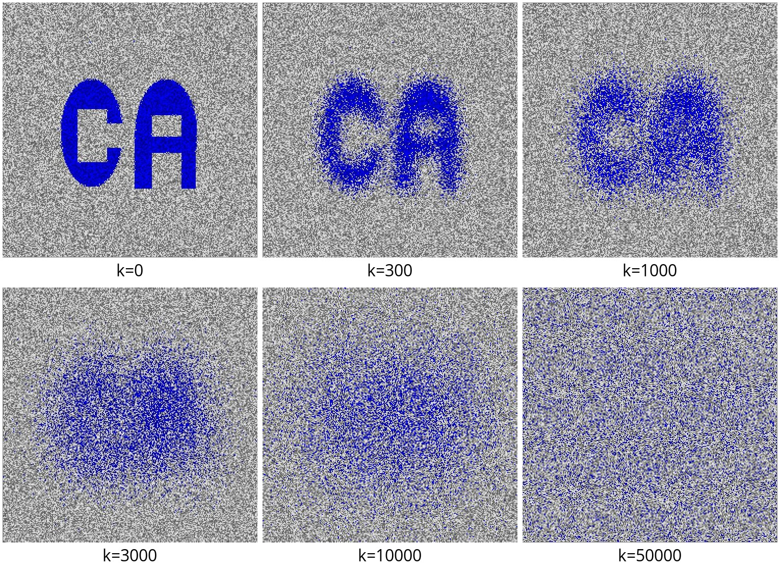
Figure 5: Patterns produced by two-dimensional diffusive rule starting from the initial image depicting letters “CA” on a lattice $250\times 250$ with periodic boundary conditions. States 0–3 are shown as shades of gray and states 4-7 as shades of blue.

5 Conclusions

Deterministic nearest-neighbour cellular automaton modelling diffusion process with very high fidelity can easily be constructed providing that sufficient number of states is employed, and in $d$ dimensions $2^{d+1}$ states are needed. This brings an interesting question and research challenge: could one construct realistic diffusion model with smaller number of states? In particular, in one dimension, can we construct a nearest-neighbour CA rule with only 3 states (instead of our 4), yet emulating diffusion process with similar quality as the rule presented here? The answer is most likely no, yet one would have to formulate the problem in a more rigorous fashion first in order to give the definitive answer. What is certain is that it cannot be done with two states, as none of the elementary CA rules exhibits sufficient diffusion-like properties.

Acknowledgements: the author acknowledges financial support from the Discovery Grant by National Science and Engineering Council of Canada.

References

- [1] Arita, C., Krapivsky, P.L., Mallick, K.: Bulk diffusion in a kinetically constrained lattice gas. Journal of Physics A Mathematical General 51(12), 125002 (2018)
- [2] Boon, J.P., Dab, D., Kapral, R., Lawniczak, A.T.: Lattice gas automata for reactive systems. Physics Reports 273(2), 55–148 (1996)
- [3] Boyce, W.E., DiPrima, R.C.: Elementary Differential Equations and Boundary Value Problems, pp. 582–583. John Wiley and Sons, Inc., New York (2001)
- [4] Chopard, B., Droz, M.: Cellular automata model for the diffusion equation. Journal of Statistical Physics 64, 859–892 (08 1991)
- [5] Chopard, B., Droz, M.: Cellular Automata Modeling of Physical Systems. Cambridge University Press, Cambridge (1998)
- [6] Fukś, H.: Solving two-dimensional density classification problem with two probabilistic cellular automata. Journal of Cellular Automata 10(1–2), 149–160 (2015)
- [7] Hardy, J., Pomeau, Y., de Pazzis, O.: Time evolution of a two-dimensional classical lattice system. Phys. Rev. Lett. 31, 276–279 (1973)
- [8] Kreyszig, E.: Advanced Engineering Mathematics, p. 570. John Wiley and Sons, Inc., New York (2011)
- [9] Medenjak, M., Klobas, K., Prosen, T.: Diffusion in deterministic interacting lattice systems. Phys. Rev. Let. 119(11), 110603 (2017)
- [10] Nava-Sedeño, J.M., Hatzikirou, H., Klages, R., Deutsch, A.: Cellular automaton models for time-correlated random walks: derivation and analysis. Scientific Reports 7, Art. no. 16952 (2017)
- [11] Rothman, D.H., Zaleski, S.: Lattice-Gas Cellular Automata: Simple Models of Complex Hydrodynamics. Cambridge University Press (1997)
- [12] Shin, S.H., Yoo, K.Y.: Analysis of 2-state, 3-neighborhood cellular automata rules for cryptographic pseudorandom number generation. In: 2009 International Conference on Computational Science and Engineering. vol. 1, pp. 399–404 (2009)
- [13] Succi, S.: The Lattice Boltzmann Equation: For Fluid Dynamics and Beyond. Clarendon Press (2001)
- [14] Trevorrow, A., Rokicki, T.: Golly (2022), http://golly.sourceforge.net/
- [15] Voroney, J.P., Lawniczak, A.T.: Construction, mathematical description and coding of reactive lattice-ggas cellular automaton. Simulation Practice and Theory 7, 657–689 (2000)
- [16] Wolf-Gladrow, D.: Lattice-Gas Cellular Automata and Lattice Boltzmann Models: An Introduction. Springer, Berlin (2004)
- [17] Wolfram, S.: Random sequence generation by cellular automata. Adv. Appl. Math. 7(2), 123–169 (1986)