Secure Full Duplex Integrated Sensing and Communications

Abstract

The following paper models a secure full duplex (FD) integrated sensing and communication (ISAC) scenario, where malicious eavesdroppers aim at intercepting the downlink (DL) as well as the uplink (UL) information exchanged between the dual functional radar and communication (DFRC) base station (BS) and a set of communication users. The DFRC BS, on the other hand, aims at illuminating radar beams at the eavesdroppers in order to sense their physical parameters, while maintaining high UL/DL secrecy rates. Based on the proposed model, we formulate a power efficient secure ISAC optimization framework design, which is intended to guarantee both UL and DL secrecy rates requirements, while illuminating radar beams towards eavesdroppers. The framework exploits artificial noise (AN) generation at the DFRC BS, along with UL/DL beamforming design and UL power allocation. We propose a beamforming design solution to the secure ISAC optimization problem. Finally, we corroborate our findings via simulation results and demonstrate the feasibility, as well as the superiority of the proposed algorithm, under different situations. We also reveal insightful trade-offs achieved by our approach.

I Introduction

Research has begun to put together a theoretical vision of 6G by looking at potential future services and applications, identifying market demands, and highlighting disruptive technologies [1]. For instance, massive machine type communications (mMTC) expects deploying one million low-price, low-power, and short-range devices, while ultra-reliable low latency communications (URLLC) targets one milli-second latency to serve mission-critical applications such as autonomous driving and remote robotic surgery. Thanks to 6G, the physical and digital worlds will be cohesively and intimately linked, eventually permeating every aspect of our lives. For that, every network provider that attempts to be trustworthy must address issues including not only high data rates and reliability but also security and privacy. According to [2], security is a state that arises from the creation and maintenance of protective measures that allow an organization to carry out its purpose or fulfill its crucial duties despite the dangers presented by threats to its usage of systems. Privacy, on the other hand, is the freedom from intrusion into a person’s private life or affairs when that intrusion is caused by the unauthorized or unlawful collection and use of data about that person [3]. Today, 5G security is a stand-alone architecture, but 6G will shift from a security-only focus to a more comprehensive view of trustworthiness, so it is crucial to integrate security capabilities with sensing and communication (SAC).

A vital component to enable future 6G systems is integrated sensing and communications (ISAC), where a common signal is used for SAC. To further highlight potential jeopardies of unsecure systems, the channel state information (CSI) contains enough details revealing critical information on a personal level from both SAC perspectives. For example, acquiring CSI reveals user keystroke information to malicious eavesdroppers [4], as well as the means to decode communicating data [5]. In particular, it is shown in [6] that a strong correlation between keystroke gestures and CSI fluctuations actually exists. In turn, broadcasting CSI information can invade privacy and create many security concerns within wireless networks. To address this problem, efforts have been made to secure wirelessly transmitted information. An instance is [7], where authors highlight the importance of privacy and the need to treat sensing parameters, in a private manner. For this, a CSI fuzzer was proposed so that only the intended receiver can perform CSI estimation, thanks to an artificial channel response added to each orthogonal frequency-division multiplexing (OFDM) transmit symbol. As a result, the receiver would estimate the overall channel impulse response, which is a cascaded version of the physical channel and the artificial one. Given the knowledge of the latter, the receiver can estimate the former. Moreover, wireless transmissions are also vulnerable to security-type attacks, for example, spoofing, due to its broadcast nature. Cryptographic approaches do offer a certain level of security in the network, however, the rapid developments made in computing power devices show that even the most mathematically complex secret key-based techniques can be broken, especially when quantum computing becomes a reality [8]. Therefore, an extra level of security should rely on physical layer design, without the need for secret-key exchange, to maintain secure transmissions especially when both SAC information are revealed to malicious users.

I-A Existing work

To begin with, [9] introduces artificial noise injection to enhance the secrecy rate of the system. In precise, artificial noise is added to the signal of interest to enrich the precoding design with additional degrees of freedom to enhance the channel capacity towards legitimate users, while deteriorating it towards malicious ones. For example, [10] leverage artificial noise injection for a single user (SU) case, where the base station (BS), termed Alice, communicates with the intended communication user, termed Bob, in the presence of a malicious eavesdropper, termed Eve. Although the work aims at maximizing the secrecy rate of the system, the problem is cast as a classical beamforming maximization problem because Eve’s rate is treated as a nuisance term throughout the optimization process, due to no prior knowledge of Eve’s CSI. Furthermore, [11] use artificial noise injection, also referred to as masked beamforming therein, for multi-user, multiple-input, multiple-output (MU-MIMO) downlink (DL) systems in the presence of only one eavesdropper and outdated CSI, whereas [12] assumes perfect CSI. The work in [13] studies hybrid cooperative beamforming strategies tailored for two-way relay networks, with the help of artificial noise injection. It has been found that the scheme not only provides extra array gain, but also blocks the jamming signal from interfering with legitimate users. In addition, the work in [14] proposes a signal-to-leakage-plus-noise ratio (SLNR) design for secure and multi-beam beamforming under a transmit power budget constraint for DL satellite communications. In addition to artificial noise, randomized beamforming was introduced in [15], where all, except the last, beamforming weights are randomized and follow realizations of the Gaussian distribution. The last element allows the legitimate user to perform secure communications, while making it impossible for malicious users to perform channel estimation. Researchers have also considered improving security performances through reconfigurable intelligent surface (RIS) technology [16, 17, 18, 19, 20]. For example, a Stackelberg game has been formulated in [16] to address energy harvesting concerns for a secure wireless powered communication network, with the aid of RIS technology. Also, [17] utilizes an RIS to improve the secrecy rate of a two-way network, and [18] makes use of RIS for non-orthogonal multiple access (NOMA). Besides beamforming on a physical layer level to maintain secrecy, efforts have also been made to maintain physical layer security through channel coding. For example, [21] investigated the application of low-density generator matrix (LDGM), a special type of low-density parity-check (LDPC), on Gaussian wiretap channels. Another instance is [22], where an LDPC variant is proposed with finite block lengths that can be combined with cryptographic codes to enhance communication security. Polar codes were also studied in the context of physical layer security [23, 24]. The aforementioned work exclusively centers on securing communication signals conveying communication information, addressing the paramount concern for security at the physical layer due to the intrinsic broadcast characteristic of wireless signals. This concern has multiplied following the advent of ISAC, creating additional security problems. Indeed, integrating sensing capabilities via communication networks unlocks unprecedented new vulnerabilities and security concerns to illegitimate sensing that must be dealt with. More specifically, ISAC signals are designed to contain both sensing, as well as communication information. Therefore, when intending to sense targets, the ISAC signal being reused for sensing would be optimized to reach the target with certain radar power characteristics. If the dual-functional radar and communication (DFRC) or ISAC BS does not account for possible suspicious activities arising due to malicious targets, then ISAC technology can be deemed insecure because of the natural communication information contained within the ISAC signal, which can be intercepted by unauthorized targets. Hence, it is crucial to model ISAC systems in the presence of potential eavesdroppers so that ISAC systems operate at their full effective capacity. Moreover, it is worth noting that efforts are being made to propose secure ISAC techniques. For example, [25] considers a single eavesdropper case, leveraging artificial noise to secure the transmitted ISAC signal from the DFRC BS for half-duplex communications, as there are no users participating in the uplink (UL), and the sensing radar design is done separately via a radar-only problem. The work in [26, 27] models a physical layer security NOMA-aided ISAC system, which exploits artificial noise (AN). In particular, a secure precoding approach was designed by maximizing the sum secrecy rate for different users through artificial jamming, and simultaneously utilizing the NOMA signals for target detection. Therefore, the DFRC/ISAC BS and users must account for revealing minimal communication information in their transmitted ISAC signal in the directions of those possibly malicious targets. Towards this security concern, the main new technical challenge when designing ISAC waveforms in full duplex (FD) cases is to carefully optimize the corresponding ISAC beamformers and the ISAC AN statistics in order to attain the three main functionalities in FD ISAC, namely sensing, communication and secrecy performance, simultaneously. In contrast to recent work on FD ISAC, our work is the first to address security concerns that can arise within FD ISAC. In this paper, we are interested in secure FD ISAC systems. The FD operation refers to a wireless system in which the same time and frequency resources are used by the DFRC BS transmitting and receiving signals from multiple DL/UL users, as well as the sensing echo. From the perspective of secure ISAC, the DFRC BS optimally transmits a secure ISAC signal, containing confidential communication information, and is also designed for secure sensing tasks, whereby sensing beams are formed towards the malicious targets through power focusing, while smartly camouflaging the communication information. Simultaneously, within the same resources, the DFRC BS receives the UL signal from communication users, superimposed onto the sensing echo. This FD operation facilitates concurrent bi-directional communication and sensing. Moreover, the FD ISAC model herein models various sources of interference arising due to the FD nature of the problem, such as the FD self interference (SI) and the UL-to-DL interference. The work in [28] has addressed FD communication ISAC from a power optimization and beamforming perspective; nonetheless, there are many differences that we want to highlight. From a sensing point of view, we have adopted the integrated sidelobe to mainlobe ratio (ISMR) radar metric to optimize the sensing performance, which can then enable us to illuminate multiple eavesdroppers, and at the same time reveal minimal communication information towards the mainlobes specified within the ISMR. The ISMR has a desirable impact not only on target detection, but also on localization performance, where power focusing can be done through the mainlobes pointing towards the eavesdroppers, while keeping low sidelobes to suppress unwanted returns, such as signal-dependent interference and clutter. Furthermore, our model captures the presence of possible malicious targets within the scene, which then enables us to define secrecy constraints for the FD ISAC scenario in both UL and DL. For this, we have adopted an AN approach, where additional parameters have to be involved in order to optimize the AN statistics, hence investing power into AN generation. Therefore, the beamformers herein, in conjunction with AN statistics and UL power levels, are designed not only to enhance communication rates, but also to improve UL and DL secrecy rates, and concisely illuminate signal power in target directions without revealing the communication information embedded in the transmitted ISAC signal. In addition, the work in [29] mainly focuses on an FD ISAC setting to model the “echo-miss” problem, which is a case arising from strong residual SI that can dominate the radar echo, hence missing the backscattered echo due to target presence. To solve this, the authors in [29] proposes an optimization problem to satisfy UL/DL communication data rates and generate transmit, receive and post-SI beamformers. It is worth noting that our work also differs in several aspects. First, the sensing metric adopted in [29] is the radar beampattern power output for one and only one target, without acknowledging clutter components. Second, and as previously mentioned, we model potential communication leaks onto multiple radar targets, which then allows us to define relevant security metrics such as UL and DL secrecy rates in our FD ISAC scheme.

I-B Contributions and Insights

This work focuses on a secure FD design, where the DFRC BS transmitting ISAC signals, designed for SAC, aims at simultaneously securing the ISAC signal in the DL and UL, in the presence of multiple eavesdroppers. To that purpose, we have summarized our contributions as follows.

• Multi-user Secure Full Duplex Model. We model an FD scenario that accommodates multiple legitimate DL and multiple legitimate UL communication users associated with a DFRC BS. Moreover, we assume multiple malicious eavesdroppers that are capable of intercepting both DL and UL communication signals exchanged between the users and DFRC BS.

• Secure ISAC Optimization Framework. Due to the FD protocol, we leverage artificial noise injection not only to improve the secrecy in the DL, but also in the UL, hence deteriorating eavesdroppers reception for both UL/DL signals. As will be shown, the artificial noise aids in creating radar beams toward the eavesdroppers so that the DFRC BS can physically sense the eavesdroppers. A power-efficient secure ISAC optimization problem is designed to achieve all the aforementioned tasks.

• Solution via successive convex approximations. Due to the non-convex nature of the secure ISAC optimization problem at hand, we resort to a successive convex approximation (SCA) technique, which enables us to exploit the non-convex optimization problem and solve it as a series of convex optimization problems. The resulting algorithm is iterative and converges with a few iterations.

• Extensive simulation results. We present extensive simulation results that demonstrate the superiority, as well as the potential of the proposed design and algorithm with respect to benchmarks, in terms of secrecy rates, and total power consumption of the FD system.

Furthermore, we unveil some important insights, i.e.

• The proposed algorithm enjoys fast convergence properties, as it requires as little as $20$ iterations to settle at a stable solution.

• We prove $\operatorname{rank}$-one optimality of the DL beamforming vectors at each iteration of the proposed SCA method. Indeed, this property is highly desired when a $\operatorname{rank}$ relaxation has been imposed at some point of an optimization problem. The advantage here is that there is no longer a necessity for post-processing methods, such as Gaussian randomization, to approximation $\operatorname{rank}-$one solutions.

• For a fixed number of eavesdroppers, the secrecy rate can settle to a stable value regardless of the number of UL and DL communication users. As compared to state-of-the-art methods, the secrecy rate can be controlled through design parameters making it less sensitive to the number of UL and DL users.

• We unveil fruitful trade-offs in terms of secure communications versus radar sensing that can be achieved with the proposed method. We show through simulations that decreasing ISMR to achieve better radar sensing performance deteriorates the secrecy performance. In addition to secure ISAC trade-offs, we also discuss power-secrecy trade-offs.

I-C Organization and Notations

The detailed structure of this paper is given as follows: Section II presents the full-duplex system model and the key performance indicators adopted in this paper. In Section III, we formulate a suitable optimization framework tailored for the secure FD ISAC design problem. The proposed algorithm is presented in Section IV. Our simulation findings are given in Section V. Finally, we conclude the paper in Section VI.

Notation: Upper-case and lower-case boldface letters denote matrices and vectors, respectively. $(.)^{T}$, $(.)^{*}$, and $(.)^{H}$ represent the transpose, the conjugate, and the transpose-conjugate operators. The statistical expectation is denoted as $\mathbb{E}\{\}$. For any complex number $z\in\mathbb{C}$, the magnitude is denoted as $|z|$, its angle is $\angle z$. The $\ell_{2}$ norm of a vector $\boldsymbol{x}$ is denoted as $\|\boldsymbol{x}\|$. The matrix $\boldsymbol{I}_{N}$ is the identity matrix of size $N\times N$. The zero-vector is $\boldsymbol{0}$. For matrix indexing, the $(i,j)^{th}$ entry of matrix $\boldsymbol{A}$ is denoted by $[\boldsymbol{A}]_{i,j}$ and its $j^{th}$ column is denoted as $[\boldsymbol{A}]_{:,j}$. The operator $\operatorname{EVD}$ stands for eigenvalue decomposition. The projector operator onto the space spanned by the columns of matrix $\boldsymbol{A}\in\mathbb{C}^{N\times M}$ is $\boldsymbol{P}_{\boldsymbol{A}}$ and the corresponding orthogonal projector is $\boldsymbol{P}_{\boldsymbol{A}}^{\perp}\triangleq\boldsymbol{I}-\boldsymbol{A}(\boldsymbol{A}^{H}\boldsymbol{A})^{-1}\boldsymbol{A}^{H}$. The $[x]^{+}$ operator returns the maximum between $x$ and $0$. A positive semi-definite matrix is denoted as $\boldsymbol{A}\succeq\boldsymbol{0}$ and a vector $\boldsymbol{x}$ with all non-negative entries is denoted as $\boldsymbol{x}\succeq\boldsymbol{0}$. The all-ones vector of appropriate dimensions is denoted by $\boldsymbol{1}$.

II System Model

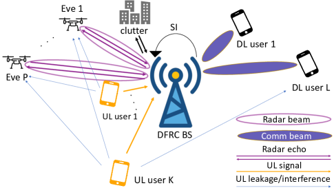
Figure 1: A practical FD ISAC scenario, in the presence of multiple malicious eavesdroppers intending to intrude on UL and DL communications between legitimate UL/DL users and a DFRC BS. Note that only one UL-to-DL interfering component is depicted, due to presentation sake.

II-A Full Duplex Radar and Communication Model

Let us assume an FD ISAC scenario, where a threat of intercepting data by malicious eavesdroppers exists in the scene. To this extent, let us first consider a DFRC BS, equipped with $N_{T}$ transmitting antennas and $N_{R}$ receiving antennas displaced via a mono-static radar setting with no isolation between both arrays. In baseband, the DFRC BS transmits the following $N_{T}\times 1$ secure ISAC signal vector

$$\boldsymbol{x}=\boldsymbol{V}\boldsymbol{s}+\boldsymbol{w},$$ (1)

where $\boldsymbol{V}\in\mathbf{C}^{N_{T}\times L}$ is the DFRC beamforming matrix, where its $\ell^{th}$ column is loaded with the beamforming vector dedicated towards the $\ell^{th}$ communication user. In addition, the total number of communication users in the DL is denoted by $L$. Moreover, $\boldsymbol{s}$ is the transmit data symbols, where its $\ell^{th}$ entry is the data symbol intended to the $\ell^{th}$ communication DL user. In what follows, the symbols are assumed to be independent with unit variance, i.e. $\mathbb{E}(\boldsymbol{s}\boldsymbol{s}^{H})=\boldsymbol{I}_{L}$. Furthermore, a superimposed AN vector, which is assumed to be independent from the signal $\boldsymbol{s}$, is transmitted via the following statistical characteristics,

$$\boldsymbol{w}\sim\mathcal{N}(\boldsymbol{0},\boldsymbol{W}),$$ (2)

where $\boldsymbol{W}\succeq\boldsymbol{0}$ stands for the spatial AN covariance matrix, which is not given and, needs to be computed. Also, $\boldsymbol{w}$ and $\boldsymbol{s}$ are assumed to be independent of one another. Note that $\operatorname{tr}(\boldsymbol{W})$ would then reflect the total transmit power invested on AN. It is worth noting that the secure ISAC signal $\boldsymbol{x}$ is not only intended for the DL users, but also is designed to be a radar signal through $\boldsymbol{V}$. Hence, $\boldsymbol{V}$ is designed for DFRC beamforming to maintain good communication properties, while preserving some radar properties that will be clarified in the paper. Moreover, the secure ISAC signal $\boldsymbol{x}$ is ”secure” in a sense that it is AN-aided through $\boldsymbol{w}$ as defined in equation (2). It is pertinent to highlight that vector $\boldsymbol{w}$ serves a dual purpose, being employed not only for AN purposes but also to augment the degrees-of-freedom (DoF) of the transmitted signal, thereby improving sensing performance. More precisely, and in what follows, the optimization process involves the participation of the covariance of $\boldsymbol{w}$, i.e. $\boldsymbol{W}$, to achieve a desired ISMR, which has positive reverberations on target detection and localization performance. We note that, as per ISAC design, this model does not specifically separate the communication and sensing signals, and so regards them as part of the same signal. Hence, the single-antenna DL communication users receive the following signal

$${y}^{\tt{DL}}_{\ell}=\sum\nolimits_{k=1}^{K}q_{k,\ell}v_{k}+\boldsymbol{h}_{r,\ell}^{H}\boldsymbol{x}+n_{\ell},\quad\ell=1\ldots L$$ (3)

where $\boldsymbol{h}_{r,\ell}$ denotes the millimeter wave (mmWave) channel between the $\ell^{th}$ DL communication user and the DFRC BS modeled as [30]

$$\boldsymbol{h}_{r,\ell}=\sqrt{\frac{\kappa_{\ell}}{\kappa_{\ell}+1}}\boldsymbol{h}_{r,\ell}^{\tt{LoS}}+\sqrt{\frac{1}{\kappa_{\ell}+1}}\boldsymbol{h}_{r,\ell}^{\tt{NLoS}}\in\mathbb{C}^{N_{T}\times 1},$$

where $\kappa_{\ell}$ is the Rician $K$-factor of the $\ell^{th}$ user. Moreover, $\boldsymbol{h}_{r,\ell}^{\tt{LoS}}$ is the line of sight (LoS) component between the $\ell^{th}$ user and the DFRC BS. In addition, the non line of sight (NLoS) component consists of $N_{\mathrm{cl}}$ clusters as follows

$$\boldsymbol{h}_{r,\ell}^{\tt{NLoS}}=\sqrt{\frac{1}{\sum_{q=1}^{N_{\mathrm{cl}}}N_{q}}}\sum_{q=1}^{N_{\mathrm{cl}}}\sum_{r=1}^{N_{q}}u_{q,r}\boldsymbol{a}_{N_{T}}(\varphi_{q,r}),$$

where $N_{q}$ is the number of propagation paths within the $q^{th}$ clusters. In addition, $u_{q,r}$ and $\varphi_{q,r}$ denote the path attenuation and angle of departures of the $r^{th}$ propagation path within the $q^{th}$ cluster. As the number of clusters grows, the path attenuation coefficients and angles between users and the DFRC BS become randomly distributed. Consequently, we model the entries of $\boldsymbol{h}_{r,\ell}^{\tt{NLoS}}$ as independently and identically distributed (i.i.d) complex Gaussian random variables [30]. In addition, $q_{k,\ell}$ is the channel coefficient between the $k^{th}$ UL communication user and the $\ell^{th}$ DL user. The interference caused by UL onto DL can be detrimental when DL/UL users are nearby one another. Moreover, the $k^{th}$ UL symbol formed by the $k^{th}$ user and intended towards the DFRC BS is denoted as $v_{k}\in\mathbb{C}$. The power level of $v_{k}$ is $\mathbb{E}(|v_{k}|^{2})=p_{k},\forall k$. Due to clutter presence, a portion of the DL signal scatters away from the clutter towards the DL communication users. Therefore, the DL channels $\boldsymbol{h}_{r,\ell}$ account for clutter. We can re-express (3) as

$${y}^{\tt{DL}}_{\ell}=\boldsymbol{h}_{r,\ell}^{H}\boldsymbol{v}_{\ell}s_{\ell}+\sum\limits_{k=1}^{K}q_{k,\ell}v_{k}+\sum\limits_{\begin{subarray}{c}\ell^{{}^{\prime}}\neq\ell\end{subarray}}^{L}\boldsymbol{h}_{r,\ell}^{H}\boldsymbol{v}_{\ell^{{}^{\prime}}}s_{\ell^{{}^{\prime}}}+\boldsymbol{h}_{r,\ell}^{H}\boldsymbol{w}+n_{\ell},$$ (4)

where the first term represents the desired part of the received signal, the second term reflects the UL-to-DL interference, the third term is the multi-user interference, the fourth noise is the jamming AN signal part and $n_{\ell}$ is zero-mean additive white Gaussian noise (AWGN) noise with variance $\sigma_{\ell}^{2}$, i.e. $n_{\ell}\sim\mathcal{N}(0,\sigma_{\ell}^{2})$.

The eavesdroppers are not only intercepting the UL signals, but also the DFRC BS DL signals. Thus, the signal at the $p^{th}$ eavesdroppers can be written as

$$y_{p}^{\tt{Eve}}=\sum\nolimits_{k=1}^{K}g_{k,p}v_{k}+\alpha_{p}\boldsymbol{a}_{N_{T}}^{H}(\theta_{p})\boldsymbol{x}+z_{p},\quad p=1\ldots P$$ (5)

where $g_{k,p}$ is the complex channel coefficient between the $k^{th}$ UL communication user and the $p^{th}$ eavesdroppers. Moreover, $\alpha_{p}$ corresponds to the path-loss complex coefficient between the DFRC BS and the $p^{th}$ eavesdropper and $\boldsymbol{a}(\theta)$ is the steering vector pointing towards angle $\theta$, i.e.

$$\boldsymbol{a}_{N_{T}}(\theta) =\begin{bmatrix}a_{1}(\theta)&\ldots&a_{N_{T}}(\theta)\end{bmatrix}^{T},$$ (6)

$$\boldsymbol{a}_{N_{R}}(\theta) =\begin{bmatrix}a_{1}(\theta)&\ldots&a_{N_{R}}(\theta)\end{bmatrix}^{T}.$$ (7)

For example, in a uniform linear antenna (ULA) setting, we have that $a_{n}(\theta)=e^{j\frac{2\pi}{\lambda}(n-1)d\sin(\theta)}$, where $\lambda$ is the wavelength. The eavesdropper angle of arrivals are denoted as $\theta_{p}$. Moreover, the AWGN at the $p^{th}$ eavesdropper is $z_{p}$, which is modeled as zero-mean and variance $\sigma_{p}^{2}$, i.e. $z_{p}\sim\mathcal{N}(0,\sigma_{p}^{2})$. We would like to highlight the relationship between the received signal at the $\ell^{th}$ legitimate DL user in (3) (equivalently (4)) and the eavesdropper in (5). We first note that both legitimate and eavesdroppers receive the UL signals, as well as the DFRC ISAC signal $\boldsymbol{x}$. However, a different channel model is adopted between the DFRC-DL, i.e. $\boldsymbol{h}_{r,\ell}$, and DFRC-eavesdropper, i.e. $\boldsymbol{a}(\theta_{p})$. This is because we regard eavesdroppers as radar targets, where a strong and dominant LoS component exists between the DFRC and the eavesdroppers (Rician channel with large $K-$factor) for localization and tracking applications. This model is applicable to scenarios involving unmanned aerial vehicles [31], [32]. More specifically, the DFRC aims at inferring additional sensing information about eavesdropping targets in the scene (such as delay and doppler), without exposing the communication information embedded within the transmit ISAC signal, $\boldsymbol{x}$. Meanwhile, a set of $K$ UL communication users associated with the DFRC BS co-exist. It is important to note that while the DFRC BS transmits a secure signal vector $\boldsymbol{x}$, it concomitantly collects the UL signals, along with other components that we shall clarify in this section, as well. Furthermore, let $\boldsymbol{h}_{t,k}$ be the UL channel vector between the $k^{th}$ UL communication user and the DFRC BS. For Rayleigh fading, the UL channels $\boldsymbol{h}_{t,k}$ also account for the clutter present in the environment, where part of the channel propagates towards the clutter and back to the DFRC BS. To this end, the signal received by the DFRC BS due to the single-antenna UL users is $\sum\nolimits_{k=1}^{K}\boldsymbol{h}_{t,k}v_{k}$.

We summarize the system model in Fig. 1, which shows a group of UL and DL legitimate communication users associated with a DFRC BS. In addition, a group of eavesdroppers listen to UL and DL signal exchanges. Note that the DL signal is an ISAC signal with the DFRC BS highlights beams towards the eavesdroppers in order to acquire physical sensing information about the eavesdroppers. Moreover, due to FD operation, the simulateneous transmission of signal vector $\boldsymbol{x}$ is ”leaked” to the receiving unit of the DFRC BS, in a form of loop interference channel. This phenomenon is referred to as SI and is one crucial component when targeting FD behavior, in particular when the transmitting and receiving units of the DFRC BS are colocated, without isolation. Indeed, the receiving unit sees an SI component of $\sqrt{\beta}\boldsymbol{H}_{\tt{SI}}\in\mathbb{C}^{N_{R}\times N_{T}}$, where $\beta$ models the residual SI power and under the direct-coupling channel model for self-interference, we have [33]

$$[\boldsymbol{H}_{\tt{SI}}]_{i,j}=\exp\Big{(}j2\pi\frac{d_{i,j}}{\lambda}\Big{)},$$ (8)

contains the phases introduced between each pair of transmitting and receiving antennas. Note that $d_{i,j}$ is the distance between the $i^{th}$ receive and $j^{th}$ transmit antennas. Furthermore, the DFRC BS aims at illuminating radar power towards the $P$ eavesdroppers. So, the echo can be modeled as

$$\boldsymbol{y}_{r}=\sum\nolimits_{p=1}^{P}\gamma_{p}\boldsymbol{a}_{N_{R}}(\theta_{p})\boldsymbol{a}_{N_{T}}^{H}(\theta_{p})\boldsymbol{x}+\boldsymbol{c}.$$ (9)

The complex amplitude due to the $p^{th}$ eavesdropper is $\gamma_{p}$ and $\boldsymbol{c}\sim\mathcal{N}(\boldsymbol{0},\boldsymbol{R}_{c})$ is the clutter including the reflected signal from the UL/DL communication users [34]. The clutter covariance matrix $\boldsymbol{R}_{c}\in\mathbb{C}^{N_{R}\times N_{R}}$ capturing all environmental clutter effects is assumed to be constant. The eavesdropper AoAs are assumed to be knowns. This a priori knowledge can be acquired through a previous estimation stage, whereby the DFRC BS uses this knowledge to design a secure FD ISAC signal. Indeed, the DFRC BS aims at estimating additional sensing parameters, like the delay for distance estimation and doppler for speed estimation, which is of interest for localization and tracking applications. In assuming partial knowledge through AoAs, the DFRC BS can further optimize its transmit signal so that the received echo is good enough, from a localization accuracy perspective [34], to further estimate/track additional sensing parameters, e.g. delay and doppler. Other ISAC works that utilize AoA target knowledge include [31] and [34]. It is worth noting that, in equation (9), due to the collocated transmit and receiving units, the AoA and AoD are the same, as vectors $\boldsymbol{a}_{N_{R}}(\theta_{p})$ and $\boldsymbol{a}_{N_{T}}^{T}(\theta_{p})$ appearing in the echo are parametrized through the same angle. Finally, the received signal at the DFRC BS is

$$\boldsymbol{y}^{\tt{DFRC}}=\sum\nolimits_{k=1}^{K}\boldsymbol{h}_{t,k}v_{k}+\boldsymbol{y}_{r}+\sqrt{\beta}\boldsymbol{H}_{\tt{SI}}\boldsymbol{x}+\boldsymbol{n}.$$ (10)

In summary, the first part in (10) is the signal due to the $K$ UL communication users. The second part highlights the received echo from the $P$ eavesdroppers, as well as environmental clutter. The third part is the SI. Finally, the AWGN vector is $\boldsymbol{n}\sim\mathcal{N}(\boldsymbol{0},\sigma_{n}^{2}\boldsymbol{I}_{N_{R}})$.

II-B Key Performance Indicators

In order to address the secure ISAC FD, it is vital to define key performance indicators (KPIs) that turn out to be essential for assessing the performance of the overall system, as well as designing a suitable optimization framework.

II-B1 Communication Achievable Rates

First, we define the signal to interference plus noise ratio (SINR) of the $\ell^{th}$ DL communication user. Based on equation (4), and under the assumption of independent symbols, we can write

$$\begin{split}&\operatorname{SINR}_{\ell}^{\tt{DL}}\\ &=\frac{\mathbb{E}\big{[}|\boldsymbol{h}_{r,\ell}^{H}\boldsymbol{v}_{\ell}s_{\ell}|^{2}\big{]}}{\sum\limits_{\begin{subarray}{c}k=1\end{subarray}}^{K}\mathbb{E}[|q_{k,\ell}v_{k}|^{2}]+\sum\limits_{\begin{subarray}{c}\ell^{{}^{\prime}}=1\\ \ell^{{}^{\prime}}\neq\ell\end{subarray}}^{L}\mathbb{E}\big{[}|\boldsymbol{h}_{r,\ell}^{H}\boldsymbol{v}_{\ell^{{}^{\prime}}}s_{\ell^{{}^{\prime}}}|^{2}\big{]}+\mathbb{E}\big{[}|\boldsymbol{h}_{r,\ell}^{H}\boldsymbol{w}|^{2}\big{]}+\sigma_{\ell}^{2}},\end{split}$$ (11)

which can also be expressed as

$$\boxed{\operatorname{SINR}_{\ell}^{\tt{DL}}=\frac{\boldsymbol{h}_{r,\ell}^{H}\boldsymbol{V}_{\ell}\boldsymbol{h}_{r,\ell}}{\sum\limits_{\begin{subarray}{c}k=1\end{subarray}}^{K}p_{k}|q_{k,\ell}|^{2}+\sum\limits_{\begin{subarray}{c}\ell^{{}^{\prime}}=1\\ \ell^{{}^{\prime}}\neq\ell\end{subarray}}^{L}\boldsymbol{h}_{r,\ell}^{H}\boldsymbol{V}_{\ell^{{}^{\prime}}}\boldsymbol{h}_{r,\ell}+\boldsymbol{h}_{r,\ell}^{H}\boldsymbol{W}\boldsymbol{h}_{r,\ell}+\sigma_{\ell}^{2}},}$$ (12)

where $\boldsymbol{V}_{\ell}=\boldsymbol{v}_{\ell}\boldsymbol{v}^{H}_{\ell}$. In this case, and according to Shannon-theory, the achievable rate of transmission of the $\ell^{th}$ DL communication user is

$$R_{\ell}^{\tt{DL}}=\log_{2}(1+\operatorname{SINR}_{\ell}^{\tt{DL}}),\quad\forall\ell=1\ldots L$$ (13)

Meanwhile, we also define an UL SINR to assess UL communication performance as seen at the DFRC BS. Assuming that the BS applies $K$ beamforming vectors $\boldsymbol{u}_{1}\ldots\boldsymbol{u}_{K}$, we can define a receive SINR quantifying the performance between the $k^{th}$ UL communication user and the DFRC BS as follows

$$\begin{split}&\operatorname{SINR}_{k}^{\tt{UL}}\\ &=\frac{\mathbb{E}[|\boldsymbol{u}_{k}^{H}\boldsymbol{h}_{t,k}v_{k}|^{2}]}{\sum\nolimits_{\begin{subarray}{c}k^{\prime}=1\\ k^{\prime}\neq k\end{subarray}}^{K}\mathbb{E}[|\boldsymbol{u}_{k}^{H}\boldsymbol{h}_{t,k^{\prime}}v_{k^{\prime}}|^{2}]+\mathbb{E}[|\boldsymbol{u}_{k}^{H}\boldsymbol{C}\boldsymbol{x}|^{2}]+\mathbb{E}[|\boldsymbol{u}_{k}^{H}\boldsymbol{c}|^{2}]+\sigma_{n}^{2}},\end{split}$$ (14)

where $\boldsymbol{C}=\sum\nolimits_{p=1}^{P}\gamma_{p}\boldsymbol{a}_{N_{R}}(\theta_{p})\boldsymbol{a}_{N_{T}}^{H}(\theta_{p})+\sqrt{\beta}\boldsymbol{H}_{\tt{SI}}$. After applying the expectation operator, we can rewrite (14) as the equation given in equation (15).

$$\boxed{\operatorname{SINR}_{k}^{\tt{UL}}=\frac{p_{k}\boldsymbol{u}_{k}^{H}\boldsymbol{h}_{t,k}\boldsymbol{h}^{H}_{t,k}\boldsymbol{u}_{k}}{\sum\nolimits_{\begin{subarray}{c}k^{\prime}=1\\ k^{\prime}\neq k\end{subarray}}^{K}p_{k^{\prime}}\boldsymbol{u}_{k}^{H}\boldsymbol{h}_{t,k^{\prime}}\boldsymbol{h}^{H}_{t,k^{\prime}}\boldsymbol{u}_{k}+\boldsymbol{u}_{k}^{H}\boldsymbol{C}\boldsymbol{Q}\boldsymbol{C}^{H}\boldsymbol{u}_{k}+\boldsymbol{u}_{k}^{H}\boldsymbol{R}_{c}\boldsymbol{u}_{k}+\sigma_{n}^{2}\boldsymbol{u}_{k}^{H}\boldsymbol{u}_{k}},}$$ (15)

In (15), $\boldsymbol{Q}=\boldsymbol{V}\boldsymbol{V}^{H}+\boldsymbol{W}$. Similarly, we can define the achievable rate of transmission of the $k^{th}$ UL communication user as

$$R_{k}^{\tt{UL}}=\log_{2}(1+\operatorname{SINR}_{k}^{\tt{UL}}),\quad\forall k=1\ldots K$$ (16)

II-B2 Secrecy Rates

Before we clearly express the secrecy rates, it is important to define the sum-rates per eavesdropper. First, we define a receive SINR between the $p^{th}$ eavesdropper and the $k^{th}$ UL communication user as follows

$$\operatorname{SINR}_{p,k}^{\tt{Eve}}=\frac{\mathbb{E}[|g_{k,p}v_{k}|^{2}]}{\sum\limits_{\begin{subarray}{c}k^{\prime}=1\\ k^{\prime}\neq k\end{subarray}}^{K}\mathbb{E}[|g_{k,p}v_{k}|^{2}]+\mathbb{E}[|\alpha_{p}\boldsymbol{a}_{N_{T}}^{H}(\theta_{p})\boldsymbol{x}|^{2}]+\mathbb{E}[|z_{p}|^{2}]},$$ (17)

which can be re-written as

$$\boxed{\operatorname{SINR}_{p,k}^{\tt{Eve}}=\frac{p_{k}|g_{k,p}|^{2}}{\sum\limits_{\begin{subarray}{c}k^{\prime}=1\\ k^{\prime}\neq k\end{subarray}}^{K}p_{k^{\prime}}|g_{k^{\prime},p}|^{2}+|\alpha_{p}|^{2}\boldsymbol{a}_{N_{T}}^{H}(\theta_{p})\boldsymbol{Q}\boldsymbol{a}_{N_{T}}(\theta_{p})+\sigma_{p}^{2}}.}$$ (18)

Similarly, we can express the receive SINR between the $p^{th}$ eavesdropper and the DFRC BS,

$$\operatorname{SINR}_{p,\tt{DFRC}}^{\tt{Eve}}=\frac{\mathbb{E}[|\alpha_{p}\boldsymbol{a}_{N_{T}}^{H}(\theta_{p})\boldsymbol{Vs}|^{2}]}{\sum\limits_{\begin{subarray}{c}k=1\end{subarray}}^{K}\mathbb{E}[|g_{k,p}v_{k}|^{2}]+\mathbb{E}[|\alpha_{p}\boldsymbol{a}^{H}_{N_{T}}(\theta_{p})\boldsymbol{w}|^{2}]+\mathbb{E}[|z_{p}|^{2}]},$$ (19)

which gives

$$\boxed{\operatorname{SINR}_{p,\tt{DFRC}}^{\tt{Eve}}=\frac{|\alpha_{p}|^{2}\boldsymbol{a}_{N_{T}}^{H}(\theta_{p})\boldsymbol{VV}^{H}\boldsymbol{a}_{N_{T}}(\theta_{p})}{\sum\limits_{\begin{subarray}{c}k=1\end{subarray}}^{K}p_{k}|g_{k,p}|^{2}+|\alpha_{p}|^{2}\boldsymbol{a}_{N_{T}}^{H}(\theta_{p})\boldsymbol{W}\boldsymbol{a}_{N_{T}}(\theta_{p})+\sigma_{p}^{2}},}$$ (20)

Now that we have defined the SINR expressions per eavesdropper, we take a step further to define the worst-case secrecy rates [35, 36, 37] of the system. Since the eavesdroppers are exposed to UL communication signals, as well as DL DFRC signals, we can define two types of worst-case secrecy rates, i.e.

$$\boxed{\operatorname{SR}_{\tt{DL}}=\min_{\ell,p}\Big{[}\log_{2}(1+\operatorname{SINR}_{\ell}^{\tt{DL}})-\log_{2}(1+\operatorname{SINR}_{p,\tt{DFRC}}^{\tt{Eve}})\Big{]}^{+},}$$ (21)

reflecting the worst-case secrecy rate of the system for DL communications, and

$$\boxed{\operatorname{SR}_{\tt{UL}}=\min_{k,p}\Big{[}\log_{2}(1+\operatorname{SINR}_{k}^{\tt{UL}})-\log_{2}(1+\operatorname{SINR}_{p,k}^{\tt{Eve}})\Big{]}^{+},}$$ (22)

reflecting the worst-case secrecy rate of the system for UL communications.

II-B3 Radar Metrics

The DFRC BS aims at performing beam management with each of its transmit vector $\boldsymbol{x}$ in order to maintain highly directional radar transmissions, which are illuminated towards the $P$ eavesdroppers, so as to extract wireless environmental features simultaneously. This allows the DFRC BS to learn physical attributes related to each one of the eavesdroppers.

In this article, we adopt the ISMR key performance indicator (KPI) [38, 39] reporting radar performance of the transmit beampattern. In fact, this ratio measures sidelobe energy to mainlobe energy as follows

$$\operatorname{ISMR}=\frac{\int\nolimits_{\boldsymbol{\Theta}_{s}}\boldsymbol{a}_{N_{T}}^{H}(\theta)\boldsymbol{R}_{\boldsymbol{xx}}\boldsymbol{a}_{N_{T}}(\theta)\ d\theta}{\int\nolimits_{\boldsymbol{\Theta}_{m}}\boldsymbol{a}_{N_{T}}^{H}(\theta)\boldsymbol{R}_{\boldsymbol{xx}}\boldsymbol{a}_{N_{T}}(\theta)\ d\theta}.$$ (23)

where $\boldsymbol{\Theta}_{s}$ and $\boldsymbol{\Theta}_{m}$ are sets containing the directions toward the side-lobe and main-lobe components, respectively. Moreover, $\boldsymbol{R}_{\boldsymbol{xx}}$ represents the transmit covariance matrix. Indeed, using equation (1), we can write

$$\boldsymbol{R}_{\boldsymbol{xx}}=\mathbb{E}(\boldsymbol{x}\boldsymbol{x}^{H})=\boldsymbol{V}\boldsymbol{V}^{H}+\boldsymbol{W}.$$ (24)

The ISMR could be reformulated after integrating over directions as

$$\operatorname{ISMR}=\frac{\operatorname{tr}\big{(}\boldsymbol{R}_{\boldsymbol{xx}}\boldsymbol{A}_{s}\big{)}}{\operatorname{tr}\big{(}\boldsymbol{R}_{\boldsymbol{xx}}\boldsymbol{A}_{m}\big{)}},$$ (25)

where $\boldsymbol{A}_{s/m}=\int\nolimits_{\boldsymbol{\Theta}_{s/m}}\boldsymbol{a}_{N_{T}}(\theta)\boldsymbol{a}_{N_{T}}^{H}(\theta)\ d\theta$. In this paper, we choose $P$ mainlobes to be centered around $\theta_{1}\ldots\theta_{P}$, respectively. The lower and upper bounds of the mainlobes are

$$\Theta_{m}=\bigcup\nolimits_{p=1}^{P}\big{\{}[\theta_{p}-\theta_{p}^{\tt{low}};\theta_{p}-\theta_{p}^{\tt{high}}]\big{\}}.$$ (26)

The ISMR metric aims at concentrating power in the mainlobe region(s), while lowering the power in the sidelobe(s) as much as possible to suppress undesired echo bounces, such as clutter and signal-dependent interference. In optimizing the beams around the target AoAs, while simultaneously attenuating clutter returns, the signal-clutter-noise ratio is improved. As a result, according to [34], the echo return can then be reliably used to estimate additional sensing parameters, such as range based on time of arrival (ToA) information and speed via doppler information. In addition to the supplementary sensing information we can estimate, the ISMR can then be adapted for tracking the targets by integrating a sophisticated tracking method to carefully steer the mainlobes defined through the ISMR. Therefore, the ISMR metric is well-suited for target localization applications and tracking. On the other hand, decreasing sidelobe powers in certain directions is, in some applications, desired in order to attenuate unwanted returns, such as interferers or clutter components. A particular and practical instance of ISMR appeared in [40], where the concept of ISMR is indirectly leveraged. In particular, a radar beamformer is optimized to receive radar signals containing clutter, where the beamformed signal enjoys a high mainlobe and a spatial sidelobe null in the direction of the clutter. But even more, the ISMR allows flexibility in the choice of how wide the mainlobes can get, which can account for uncertainty on the eavesdropper locations. More specifically, the uncertainty on the $p^{th}$ eavesdropper AoA can be accomodated by appropriately configuring $\theta_{p}^{\tt{low}}$ and $\theta_{p}^{\tt{high}}$. It is worth noting that the ISMR has also been adopted in several works, i.e. [41], [42], and [43]. It is worthwhile pausing here and observing that we are faced with a ”push-pull” type problem. On one hand, the DFRC BS aims at probing for energy focusing, in order to extract physical sensing parameters of the eavesdroppers by illuminating simultaneous radar beams centered around locations $\theta_{1}\ldots\theta_{P}$. But, on the other hand, the DFRC BS also aims at revealing minimal communication information towards the malicious eavesdroppers through proper AN covariance design.

III Optimization Framework for Secure ISAC

In this section, we devise an ISAC optimization problem intended for total power minimization that is to be invested on the UL power allocation, DL beamforming, as well as AN generation. We would like to mention that, as highlighted by [44], the ideal case where perfect CSI is available at the transmitter, the achievable secrecy rate can be made arbitrarily large by increasing the transmission power. From a power efficiency perspective, though, we intend to find the best power allocation strategy satisfying the UL and DL achievable secrecy rates. However, to accommodate for ISAC and secrecy rate constraints, power minimization takes place under UL and DL secrecy rates, while guaranteeing a maximum ISMR. Based on this, we propose the following optimization problem,

$$(\mathcal{P}_{1}):\begin{cases}\min\limits_{\{\begin{subarray}{c}\boldsymbol{U},\boldsymbol{V},\boldsymbol{W},\boldsymbol{p}\end{subarray}\}}&\operatorname{tr}(\boldsymbol{VV}^{H})+\operatorname{tr}(\boldsymbol{W})+\sum\nolimits_{k=1}^{K}p_{k}\\ \textrm{s.t.}&\operatorname{SR}_{\tt{DL}}\geq\rho^{\tt{DL}},\\ &\operatorname{SR}_{\tt{UL}}\geq\rho^{\tt{UL}},\\ &\operatorname{ISMR}\leq\operatorname{ISMR}_{\tt{max}},\\ &\boldsymbol{W}\succeq\boldsymbol{0},\ \boldsymbol{p}\succeq\boldsymbol{0}.\\ \end{cases}$$ (27)

For convenience, $\boldsymbol{U}\in\mathbb{C}^{N_{R}\times K}$ contains $\boldsymbol{u}_{k}$ in its $k^{th}$ column and $\boldsymbol{p}$ is a power vector containing $p_{k}$ in its $k^{th}$ entry. We first discuss the optimization problem along with its constraints before solving the problem. In particular, we aim at economizing the total transmit power that is to-be invested in DFRC operation, AN-noise, as well as total power transmitted in the UL over all users. Furthermore, we target a minimum acceptable UL/DL worst-case secrecy rate, captured by the first two constraints, which reflects the amount of information-leakage towards the malicious eavesdroppers. In this context, $\rho^{\tt{DL}}$ and $\rho^{\tt{UL}}$ denote predefined tolerance thresholds for the worst-case secrecy rates in the DL and UL, respectively. Moreover, the optimization should take place under a maximal ISMR, defined hereby through the parameter $\operatorname{ISMR}_{\tt{max}}$, in order to sustain proper radar beams towards the eavesdroppers. This shall guarantee minimum communication information revealed to the eavesdroppers, relative to the DFRC BS and the DL users, while at the same time illuminating beams towards the former. Due to the non-convexity of the secrecy rate constraints, we cast problem (27) as follows

$$(\mathcal{P}_{1.1}):\begin{cases}\min\limits_{\{\begin{subarray}{c}\boldsymbol{U},\boldsymbol{V},\boldsymbol{W},\boldsymbol{p}\end{subarray}\}}&\operatorname{tr}(\boldsymbol{VV}^{H})+\operatorname{tr}(\boldsymbol{W})+\boldsymbol{1}^{T}\boldsymbol{p}\\ \textrm{s.t.}&\operatorname{SINR}_{\ell}^{\tt{DL}}\geq\zeta_{\ell}^{\tt{DL}},\quad\forall\ell,\\ &\operatorname{SINR}_{k}^{\tt{UL}}\geq\zeta_{k}^{\tt{UL}},\quad\forall k,\\ &\operatorname{SINR}_{p,\tt{DFRC}}^{\tt{Eve}}\leq\zeta_{p,\tt{DFRC}}^{\tt{Eve}},\quad\forall p,\\ &\operatorname{SINR}_{p,k}^{\tt{Eve}}\leq\zeta_{p,k}^{\tt{Eve}},\quad\forall p,k\\ &\operatorname{ISMR}\leq\operatorname{ISMR}_{\tt{max}},\\ &\boldsymbol{W}\succeq\boldsymbol{0},\ \boldsymbol{p}\succeq\boldsymbol{0},\\ \end{cases}$$ (28)

where now we define $\zeta_{\ell}^{\tt{DL}}$ and $\zeta_{k}^{\tt{UL}}$ as the minimum accepted SINR of the $\ell^{th}$ DL and $k^{th}$ UL communication users, respectively. Meanwhile, the maximum accepted SINR of the $p^{th}$ eavesdropper relative to the DFRC is $\zeta_{p,\tt{DFRC}}^{\tt{Eve}}$, and the maximum accepted SINR of the $p^{th}$ eavesdropper relative to the $k^{th}$ UL communication user is $\zeta_{p,k}^{\tt{Eve}}$. To see the equivalence between the two problems in equations (27) and (28), we define $LP$ positive real numbers of the form $\{\rho^{\tt{DL}}_{\ell,p}\}_{\begin{subarray}{c}\ell=1\ldots L\\ p=1\ldots P\end{subarray}}$ taking the form of

$$\rho^{\tt{DL}}_{\ell,p}=\log_{2}(1+\zeta_{\ell}^{\tt{DL}})-\log_{2}(1+\zeta_{p,\tt{DFRC}}^{\tt{Eve}}),\quad\forall\ell,p$$ (29)

where $\min\nolimits_{\ell,p}\rho^{\tt{DL}}_{\ell,p}=\rho^{\tt{DL}}$ and $\zeta_{\ell}^{\tt{DL}}>\zeta_{p,\tt{DFRC}}^{\tt{Eve}}$. Next, using the definition of DL worst-case secrecy rate in equation (21) on the first constraint of problem (27), we get

$$\log_{2}(1+\operatorname{SINR}_{\ell}^{\tt{DL}})-\log_{2}(1+\operatorname{SINR}_{p,\tt{DFRC}}^{\tt{Eve}})\geq\rho^{\tt{DL}}_{\ell,p},\quad\forall\ell,p$$ (30)

Finally, using (29) in (30), we can satisfy the first constraint in (27) by upper bounding $\operatorname{SINR}_{\ell}^{\tt{DL}}$ through the first constraint of (28), and lower bounding $\operatorname{SINR}_{p,\tt{DFRC}}^{\tt{Eve}}$ through the third constraint of (28). A similar argument is used by utilizing the definition of the UL worst-case secrecy rate in equation (22) to arrive at the second and fourth constraints appearing in problem (28). In the following section, we propose an iterative method to solve (28).

IV Secure ISAC via Successive Convex Approximations

IV-A Algorithmic Derivation

We start by optimizing with respect to $\boldsymbol{U}$. Note that the only quantities depending on $\boldsymbol{U}$ are $\{\operatorname{SINR}_{k}^{\tt{UL}}\}_{k=1}^{K}$. Therefore, we first aim to maximize all the UL SINRs with respect to $\boldsymbol{U}$. Based on this, we consider

$$\Big{\{}\widehat{\boldsymbol{U}}=\operatorname*{arg\,max}_{\boldsymbol{U}}\sum\limits_{k=1}^{K}\operatorname{SINR}_{k}^{\tt{UL}}\Big{\}}\propto\Big{\{}\widehat{\boldsymbol{u}}_{k}=\operatorname*{arg\,max}_{\boldsymbol{u}_{k}}\operatorname{SINR}_{k}^{\tt{UL}}\Big{\}}.$$ (31)

Note that $\operatorname{SINR}_{k}^{\tt{UL}}$ forms a generalized Rayleigh quotient in $\boldsymbol{u}_{k}$ taking the form of

$$\begin{split}&\operatorname{SINR}_{k}^{\tt{UL}}\\ &=\frac{p_{k}\boldsymbol{u}_{k}^{H}\boldsymbol{h}_{t,k}\boldsymbol{h}^{H}_{t,k}\boldsymbol{u}_{k}}{\boldsymbol{u}_{k}^{H}\Bigg{(}\sum\nolimits_{\begin{subarray}{c}k^{\prime}=1\\ k^{\prime}\neq k\end{subarray}}^{K}p_{k^{\prime}}\boldsymbol{h}_{t,k^{\prime}}\boldsymbol{h}^{H}_{t,k^{\prime}}+\boldsymbol{C}\boldsymbol{Q}\boldsymbol{C}^{H}+\boldsymbol{R}_{c}+\sigma_{n}^{2}\boldsymbol{I}\Bigg{)}\boldsymbol{u}_{k}}.\quad\forall k\end{split}$$ (32)

Following [45], the solution of the optimization problem in (31) is readily obtained via

$$\small\begin{split}\widehat{\boldsymbol{u}}_{k}\propto\max\operatorname{eigvec}\Bigg{[}\Bigg{(}\sum\limits_{\begin{subarray}{c}k^{\prime}=1\\ k^{\prime}\neq k\end{subarray}}^{K}&p_{k^{\prime}}\boldsymbol{h}_{t,k^{\prime}}\boldsymbol{h}^{H}_{t,k^{\prime}}+\boldsymbol{C}\boldsymbol{Q}\boldsymbol{C}^{H}+\boldsymbol{R}_{c}+\sigma_{n}^{2}\boldsymbol{I}\Bigg{)}^{-1}\\ &\boldsymbol{h}_{t,k}\boldsymbol{h}^{H}_{t,k}\Bigg{]},\forall k=1\ldots K.\end{split}$$ (33)

But since $\boldsymbol{h}_{t,k}\boldsymbol{h}^{H}_{t,k}$ is $\operatorname{rank}$-one, then the optimal beamforming vector maximizing the SINR at the $k^{th}$ UL communication user can be expressed as

$$\widehat{\boldsymbol{u}}_{k}=\Bigg{(}\sum\nolimits_{\begin{subarray}{c}k^{\prime}=1\\ k^{\prime}\neq k\end{subarray}}^{K}p_{k^{\prime}}\boldsymbol{h}_{t,k^{\prime}}\boldsymbol{h}^{H}_{t,k^{\prime}}+\boldsymbol{C}\boldsymbol{Q}\boldsymbol{C}^{H}+\boldsymbol{R}_{c}+\sigma_{n}^{2}\boldsymbol{I}\Bigg{)}^{-1}\boldsymbol{h}_{t,k},$$ (34)

Treating $\widehat{\boldsymbol{u}}_{k}$ as nuisance parameters, we plug their expressions back in (28) to get a problem independent of $\boldsymbol{U}$ as

$$(\mathcal{P}_{1.2}):\begin{cases}\min\limits_{\{\begin{subarray}{c}\boldsymbol{V},\boldsymbol{W},\boldsymbol{p}\end{subarray}\}}&\sum\nolimits_{\ell=1}^{L}\operatorname{tr}(\boldsymbol{\boldsymbol{V}}_{\ell})+\operatorname{tr}(\boldsymbol{W})+\boldsymbol{1}^{T}\boldsymbol{p}\\ \textrm{s.t.}&\operatorname{SINR}_{\ell}^{\tt{DL}}\geq\zeta_{\ell}^{\tt{DL}},\quad\forall\ell,\\ &\widehat{\operatorname{SINR}}_{k}^{\tt{UL}}\geq\zeta_{k}^{\tt{UL}},\quad\forall k,\\ &\operatorname{SINR}_{p,\tt{DFRC}}^{\tt{Eve}}\leq\zeta_{p,\tt{DFRC}}^{\tt{Eve}},\quad\forall p,\\ &\operatorname{SINR}_{p,k}^{\tt{Eve}}\leq\zeta_{p,k}^{\tt{Eve}},\quad\forall p,k\\ &\operatorname{ISMR}\leq\operatorname{ISMR}_{\tt{max}},\\ &\boldsymbol{W}\succeq\boldsymbol{0},\ \boldsymbol{p}\succeq\boldsymbol{0},\ \boldsymbol{V}_{\ell}\succeq\boldsymbol{0},\quad\forall\ell\\ &\operatorname{rank}(\boldsymbol{V}_{\ell})=1,\quad\forall\ell\end{cases}$$ (35)

where the UL SINR of the $k^{th}$ user after beamforming as seen by the DFRC BS is given as

$$\begin{split}&\widehat{\operatorname{SINR}}_{k}^{\tt{UL}}\\ &=p_{k}\boldsymbol{h}^{H}_{t,k}\Bigg{(}\sum\limits_{\begin{subarray}{c}k^{\prime}=1\\ k^{\prime}\neq k\end{subarray}}^{K}p_{k^{\prime}}\boldsymbol{h}_{t,k^{\prime}}\boldsymbol{h}^{H}_{t,k^{\prime}}+\boldsymbol{C}\boldsymbol{Q}\boldsymbol{C}^{H}+\boldsymbol{R}_{c}+\sigma_{n}^{2}\boldsymbol{I}\Bigg{)}^{-1}\boldsymbol{h}_{t,k}.\end{split}$$ (36)

Note that we have replaced the term $\operatorname{tr}(\boldsymbol{VV}^{H})$ by $\sum\nolimits_{\ell=1}^{L}\operatorname{tr}(\boldsymbol{\boldsymbol{V}}_{\ell})$, where each $\boldsymbol{\boldsymbol{V}}_{\ell}$ is constrained to be rank-one. The first constraint in (35) is written in terms of traces as,

$$\begin{split}\operatorname{tr}\{\big{(}\frac{1}{\zeta_{\ell}^{\tt{DL}}}\boldsymbol{V}_{\ell}-(\sum\limits_{\begin{subarray}{c}\ell^{{}^{\prime}}\neq\ell\end{subarray}}^{L}\boldsymbol{V}_{\ell^{\prime}}+\boldsymbol{W})\big{)}\boldsymbol{H}_{r,\ell}\}\geq\Big{(}\sum\limits_{\begin{subarray}{c}k=1\end{subarray}}^{K}p_{k}|q_{k,\ell}|^{2}+\sigma_{\ell}^{2}\Big{)},\end{split}$$ (37)

where $\boldsymbol{H}_{r,\ell}=\boldsymbol{h}_{r,\ell}\boldsymbol{h}_{r,\ell}^{H}$, which describes a convex set. The second constraint in (35) is non-convex. To remedy this non-convexity, we resort to the SCA technique to relax the non-convex constraint. Thus, via sequential convex programming in an iterative fashion, we can provide a locally optimal solution. Before we proceed, we write the second constraint in (35) as

$$p_{k}\boldsymbol{h}^{H}_{t,k}\boldsymbol{\Phi}_{k}^{-1}(\boldsymbol{Q},\boldsymbol{p})\boldsymbol{h}_{t,k}\geq\zeta_{k}^{\tt{UL}},\quad\forall k=1\ldots K,$$ (38)

where $\boldsymbol{\Phi}_{k}(\boldsymbol{Q},\boldsymbol{p})=\sum\nolimits_{\begin{subarray}{c}k^{\prime}=1\\ k^{\prime}\neq k\end{subarray}}^{K}p_{k^{\prime}}\boldsymbol{h}_{t,k^{\prime}}\boldsymbol{h}^{H}_{t,k^{\prime}}+\boldsymbol{C}\boldsymbol{Q}\boldsymbol{C}^{H}+\boldsymbol{R}_{c}+\sigma_{n}^{2}\boldsymbol{I}.$ Now, exploring the following first-order Taylor series approximation about a given estimate of $\boldsymbol{\Phi}_{k}^{-1}(\boldsymbol{Q},\boldsymbol{p})$, say $[\boldsymbol{\Phi}_{k}^{(m)}]^{-1}\triangleq\boldsymbol{\Phi}_{k}^{-1}(\boldsymbol{Q}^{(m)},\boldsymbol{p}^{(m)})$, which is the obtained estimate of $\boldsymbol{\Phi}_{k}^{-1}(\boldsymbol{Q},\boldsymbol{p})$ at the $m^{th}$ iteration of the SCA method,

$$\begin{split}&\boldsymbol{h}^{H}_{t,k}\boldsymbol{\Phi}_{k}^{-1}(\boldsymbol{Q},\boldsymbol{p})\boldsymbol{h}_{t,k}\geq\boldsymbol{h}^{H}_{t,k}[\boldsymbol{\Phi}_{k}^{(m)}]^{-1}\boldsymbol{h}_{t,k}\\ &-\boldsymbol{h}^{H}_{t,k}[\boldsymbol{\Phi}_{k}^{(m)}]^{-1}\big{(}\boldsymbol{\Phi}_{k}-\boldsymbol{\Phi}_{k}^{(m)}\big{)}[\boldsymbol{\Phi}_{k}^{(m)}]^{-1}\boldsymbol{h}_{t,k}.\end{split}$$ (39)

Using the above lower-bound to upper-bound $\zeta_{k}^{\tt{UL}}$ for all $k=1\ldots K$, we can write at iteration $m$ the following

$$\begin{split}\boldsymbol{\Lambda}_{k}\leq 0,\ \forall k=1\ldots k.\end{split}$$ (40)

where $\boldsymbol{\Lambda}_{k}=\frac{\zeta_{k}^{\tt{UL}}}{p_{k}}+\boldsymbol{h}^{H}_{t,k}[\boldsymbol{\Phi}_{k}^{(m)}]^{-1}\boldsymbol{\Phi}_{k}[\boldsymbol{\Phi}_{k}^{(m)}]^{-1}\boldsymbol{h}_{t,k}-2\boldsymbol{h}^{H}_{t,k}[\boldsymbol{\Phi}_{k}^{(m)}]^{-1}\boldsymbol{h}_{t,k}$. The first order derivatives of $\boldsymbol{\Lambda}_{k}$ are

$$\frac{\partial\boldsymbol{\Lambda}_{k}}{\partial p_{k}} =-\frac{\zeta_{k}^{\tt{UL}}}{p_{k}^{2}},$$

$$\frac{\partial\boldsymbol{\Lambda}_{k}}{\partial p_{k^{\prime}}} =\boldsymbol{h}^{H}_{t,k}[\boldsymbol{\Phi}_{k}^{(m)}]^{-1}\boldsymbol{h}_{t,k^{\prime}}\boldsymbol{h}_{t,k^{\prime}}^{H}[\boldsymbol{\Phi}_{k}^{(m)}]^{-1}\boldsymbol{h}_{t,k},\quad\forall k^{\prime}\neq k,$$

$$\frac{\partial\boldsymbol{\Lambda}_{k}}{\partial\boldsymbol{V}_{\ell}} =\frac{\partial\boldsymbol{\Lambda}_{k}}{\partial\boldsymbol{W}}=\boldsymbol{C}^{H}[\boldsymbol{\Phi}_{k}^{(m)}]^{-1}\boldsymbol{h}_{t,k}\boldsymbol{h}_{t,k}^{H}[\boldsymbol{\Phi}_{k}^{(m)}]^{-1}\boldsymbol{C},\quad\forall\ell.$$

As the expression $\boldsymbol{\Lambda}_{k}$ is twice differentiable, we can see that from the above expressions, all second-order derivatives are zero, except for

$$\frac{\partial^{2}\boldsymbol{\Lambda}_{k}}{\partial p_{k}^{2}}=\frac{2\zeta_{k}^{\tt{UL}}}{p_{k}^{3}}.$$ (41)

This means that the Hessian $\nabla^{2}\boldsymbol{\Lambda}_{k}$ is an all-zero matrix except for $\frac{2\zeta_{k}^{\tt{UL}}}{p_{k}^{3}}$ at its $k^{th}$ diagonal entry. Therefore, $\nabla^{2}\boldsymbol{\Lambda}_{k}\succeq\boldsymbol{0}$ if and only if $\frac{2\zeta_{k}^{\tt{UL}}}{p_{k}^{3}}\geq 0$, which is valid since the powers $p_{k}$ are constrained to be positive and $\zeta_{k}^{\tt{UL}}$ is a given positive quantity. Finally, we conclude that $\boldsymbol{\Lambda}_{k}$ is convex in $\boldsymbol{p}$, $\boldsymbol{V}_{1}\ldots\boldsymbol{V}_{L}$ and $\boldsymbol{W}$. Moreover, the third constraint in (35) is written as

$$\begin{split}&\frac{1}{\zeta_{p,\tt{DFRC}}^{\tt{Eve}}}|\alpha_{p}|^{2}\boldsymbol{a}_{N_{T}}^{H}(\theta_{p})\Big{(}\sum\nolimits_{\ell=1}^{L}\operatorname{tr}(\boldsymbol{\boldsymbol{V}}_{\ell})\Big{)}\boldsymbol{a}_{N_{T}}(\theta_{p})\\ &\leq\sum\nolimits_{\begin{subarray}{c}k=1\end{subarray}}^{K}p_{k}|g_{k,p}|^{2}+|\alpha_{p}|^{2}\boldsymbol{a}_{N_{T}}^{H}(\theta_{p})\boldsymbol{W}\boldsymbol{a}_{N_{T}}(\theta_{p})+\sigma_{p}^{2},\end{split}$$ (42)

where, as done on the objective function, we have replaced $\boldsymbol{VV}^{H}$ with $\sum\nolimits_{\ell=1}^{L}\operatorname{tr}(\boldsymbol{\boldsymbol{V}}_{\ell})$. Furthermore, the fourth constraint in (35) can be expressed as follows

$$\begin{split}&\frac{1}{\zeta_{p,k}^{\tt{Eve}}}p_{k}|g_{k,p}|^{2}\\ &-\Big{(}\sum\limits_{\begin{subarray}{c}k^{\prime}\neq k\end{subarray}}^{K}p_{k^{\prime}}|g_{k^{\prime},p}|^{2}+|\alpha_{p}|^{2}\boldsymbol{a}_{N_{T}}^{H}(\theta_{p})\boldsymbol{Q}\boldsymbol{a}_{N_{T}}(\theta_{p})+\sigma_{p}^{2}\Big{)}\leq 0.\end{split}$$ (43)

Finally, dropping the $\operatorname{rank}-$one constraint in the $m^{th}$ iteration of the SCA method, the optimization problem in (35) can be translated to (46). As shall be seen in the next section, the $\operatorname{rank}-$one relaxation does not introduce a sub-optimality due to the special structure of the optimization problem in hand.

Note that problem $(\mathcal{P}_{1.3}^{(m)})$ is a convex optimization problem and can be readily solved via classical solvers, e.g., the CVX toolbox in MATLAB. Before we summarize our SCA-based algorithm, we introduce an optimality theorem related to the optimization problem at hand, which will further aid us at generating the beamforming vectors. The implicit presence of perfect CSI knowledge at all given nodes in an ISAC system is a simplifying assumption. In reality, this knowledge cannot be perfect as inaccurate estimation and quantization errors, as well as outdated channel effects, are part of transmit and receive paths. The imperfect CSI case can be accommodated as part of this design by leveraging the ellipsoidal error model on the available CSI vectors. For example, we can model $\boldsymbol{h}_{r,\ell}=\widehat{\boldsymbol{h}}_{r,\ell}+\Delta\boldsymbol{h}_{r,\ell}$, where $\|\boldsymbol{E}_{r,\ell}^{\frac{1}{2}}\Delta\boldsymbol{h}_{r,\ell}\|\leq 1$ for all $\ell$. Here, $\boldsymbol{E}_{r,\ell}$ controls the ellipsoidal shape of the CSI perturbation set on the $\ell^{th}$ DL channel. A similar model can be adopted for all other links. Furthermore, a block cyclic coordinate descent (BCCD) type algorithm can be further devised due to the decoupled nature of some constraints that follow due to the imperfect CSI formulation. However, due to lack of space, we defer the imperfect CSI extension of the proposed secure FD ISAC problem as part of our future work.

Algorithm 1 SCA-based method to optimize (27)

  

  Input: $\{\zeta_{\ell}^{\tt{DL}},\boldsymbol{h}_{r,\ell},\sigma_{\ell}\}_{\ell=1}^{L}$, $\{\zeta_{k}^{\tt{UL}},\boldsymbol{h}_{t,k}\}_{k=1}^{K}$, $\{\zeta_{p,\tt{DFRC}}^{\tt{Eve}},\gamma_{p},\theta_{p},\sigma_{p},\alpha_{p}\}_{p=1}^{P}$, $\{\zeta_{p,k}^{\tt{Eve}},g_{k,p}\}_{p,k=1}^{P,K}$, $\operatorname{ISMR}_{\tt{max}}$, $\beta$, $\boldsymbol{H}_{\tt{SI}}$, $\boldsymbol{A}_{s}$, $\boldsymbol{A}_{m}$.

  Initialize:

        Set $m=0$, $\boldsymbol{V}_{\ell}^{(0)}=\boldsymbol{I}$, $\boldsymbol{W}^{(0)}=\boldsymbol{0}$, $\boldsymbol{p}^{(0)}=\frac{1}{K}\boldsymbol{1}$.

        Compute $\boldsymbol{C}=\sum\nolimits_{p=1}^{P}\gamma_{p}\boldsymbol{a}_{N_{R}}(\theta_{p})\boldsymbol{a}_{N_{T}}^{H}(\theta_{p})+\sqrt{\beta}\boldsymbol{H}_{\tt{SI}}$.

  while $m<M_{iter}$

        Solve $(\mathcal{P}_{1.3}^{(m)})$ in (46) to get $\boldsymbol{V}_{\ell}^{(m+1)},\boldsymbol{W}^{(m+1)},\boldsymbol{p}^{(m+1)}$.

        Update $\boldsymbol{Q}^{(m+1)}$ as $\boldsymbol{Q}^{(m+1)}=\sum\nolimits_{\ell=1}^{L}\boldsymbol{V}_{\ell}^{(m+1)}+\boldsymbol{W}^{(m+1)}$.

        Update $\boldsymbol{\Phi}_{k}^{(m+1)}$ for all $k$ as

        $m\leftarrow m+1$

        $\boldsymbol{\Phi}_{k}^{(m)}=\sum\limits_{\begin{subarray}{c}k^{\prime}=1\\ k^{\prime}\neq k\end{subarray}}^{K}p_{k^{\prime}}^{(m)}\boldsymbol{h}_{t,k^{\prime}}\boldsymbol{h}^{H}_{t,k^{\prime}}+\boldsymbol{C}\boldsymbol{Q}^{(m)}\boldsymbol{C}^{H}+\boldsymbol{R}_{c}+\sigma_{n}^{2}\boldsymbol{I}$.

  set $\widehat{\boldsymbol{Q}}=\boldsymbol{Q}^{(m)}$, $\widehat{\boldsymbol{W}}=\boldsymbol{W}^{(m)}$, $\widehat{\boldsymbol{p}}=\boldsymbol{p}^{(m)}$, $\{\widehat{\boldsymbol{V}}_{\ell}={\boldsymbol{V}}_{\ell}^{(m)}\}_{\ell=1}^{L}$.

  for $k=1\ldots K$

        $\widehat{\boldsymbol{u}}_{k}=\Bigg{(}\sum\limits_{\begin{subarray}{c}k^{\prime}=1\\ k^{\prime}\neq k\end{subarray}}^{K}\widehat{p}_{k^{\prime}}\boldsymbol{h}_{t,k^{\prime}}\boldsymbol{h}^{H}_{t,k^{\prime}}+\boldsymbol{C}\widehat{\boldsymbol{Q}}\boldsymbol{C}^{H}+\boldsymbol{R}_{c}+\sigma_{n}^{2}\boldsymbol{I}\Bigg{)}^{-1}\boldsymbol{h}_{t,k}$.

  for $\ell=1\ldots L$

        $\lambda_{\ell}\boldsymbol{v}_{\ell}\boldsymbol{v}_{\ell}^{H}\leftarrow\operatorname{EVD}\big{(}{\boldsymbol{V}}_{\ell}^{(M_{iter})}\big{)}$.

        $\widehat{\boldsymbol{V}}_{[:,\ell]}\leftarrow\sqrt{\lambda_{\ell}}\boldsymbol{v}_{\ell}$.

  return $\{\widehat{\boldsymbol{u}}_{k}\}_{k=1}^{K}$, $\widehat{\boldsymbol{W}}$, $\widehat{\boldsymbol{p}}$, $\widehat{\boldsymbol{V}}$.

IV-B Optimality

Ideally, we would aim to produce DL $\operatorname{rank}-$one beamforming solutions of the form $\boldsymbol{v}_{\ell}\boldsymbol{v}_{\ell}^{H}$. Otherwise, post-processing procedures are required to produce $\operatorname{rank}$-one approximations of $\boldsymbol{V}_{\ell}$, $\forall\ell$. Accordingly, Gaussian randomization techniques or principle component analysis methods are commonly employed to obtain a suboptimal solution. These approximations include Gaussian randomization [46, 47]. However, in our case, due to the special structure of the problem, we have the following result.

Theorem 1 ($\operatorname{rank}$-one Optimality): At the $m^{th}$ iteration of Algorithm 1, consider the optimization problem $(\mathcal{P}_{1.3}^{(m)})$ given in equation (46). Then, for all $\ell=1\ldots L$, the solution of $(\mathcal{P}_{1.3}^{(m)})$ satisfies

$$\operatorname{rank}(\boldsymbol{V}_{\ell}^{(m)})=1,\quad\forall\ell=1\ldots L.$$ (44)

The proof of this theorem is detailed in Appendix A. It turns out that our relaxation is not a ”relaxation”, after all. Given the $\operatorname{rank}-$one optimality of $\operatorname{rank}(\boldsymbol{V}_{1}^{(m)})\ldots\operatorname{rank}(\boldsymbol{V}_{L}^{(m)})$, an eigenvalue decomposition (EVD) suffices to recover $\boldsymbol{V}$. This is achieved as follows

$$\boldsymbol{V}_{[:,\ell]}=\sqrt{\lambda_{\ell}^{(\infty)}}\boldsymbol{v}_{\ell}^{(\infty)},$$ (45)

where $\lambda_{\ell}^{(\infty)}$ and $\boldsymbol{v}_{\ell}^{(\infty)}$ represent the non-zero eigenvalue and its corresponding eigenvector of the final converged quantity given by Algorithm 1, i.e. $\boldsymbol{V}_{\ell}^{(\infty)}$, respectively. The above theorem tells us that the $\operatorname{rank}$-one relaxation does not introduce any sort of sub-optimality onto the relaxed problem. An instance of such an optimality appears in [43], where ISAC beamforming was used to study outage performances in the case of imperfect channel state information. Furthermore, thanks to this theorem, we can now generate the DL beamforming vectors through EVD. To this end, the proposed algorithm is summarized in Algorithm 1.

$$(\mathcal{P}_{1.3}^{(m)}):\begin{cases}\min\limits_{\big{\{}\begin{subarray}{c}\boldsymbol{V}_{1}\ldots\boldsymbol{V}_{L},\\ \boldsymbol{W},\boldsymbol{p}\end{subarray}\big{\}}}&\sum\nolimits_{\ell=1}^{L}\operatorname{tr}(\boldsymbol{\boldsymbol{V}}_{\ell})+\operatorname{tr}(\boldsymbol{W})+\boldsymbol{1}^{T}\boldsymbol{p}\\ \textrm{s.t.}&\frac{1}{\zeta_{\ell}^{\tt{DL}}}\operatorname{tr}(\boldsymbol{V}_{\ell}\boldsymbol{H}_{r,\ell})-\Big{(}\sum\nolimits_{\begin{subarray}{c}k=1\end{subarray}}^{K}p_{k}|q_{k,\ell}|^{2}+\sum\nolimits_{\begin{subarray}{c}\ell^{{}^{\prime}}\neq\ell\end{subarray}}\operatorname{tr}(\boldsymbol{V}_{\ell^{\prime}}\boldsymbol{H}_{r,\ell})+\operatorname{tr}(\boldsymbol{W}\boldsymbol{H}_{r,\ell})+\sigma_{\ell}^{2}\Big{)}\geq 0,\quad\forall\ell=1\ldots L,\\ &\frac{\zeta_{k}^{\tt{UL}}}{p_{k}}+\boldsymbol{h}^{H}_{t,k}[\boldsymbol{\Phi}_{k}^{(m)}]^{-1}\boldsymbol{\Phi}_{k}[\boldsymbol{\Phi}_{k}^{(m)}]^{-1}\boldsymbol{h}_{t,k}-2\boldsymbol{h}^{H}_{t,k}[\boldsymbol{\Phi}_{k}^{(m)}]^{-1}\boldsymbol{h}_{t,k}\leq 0,\quad\forall k=1\ldots K,\\ &\frac{1}{\zeta_{p,\tt{DFRC}}^{\tt{Eve}}}|\alpha_{p}|^{2}\boldsymbol{a}_{N_{T}}^{H}(\theta_{p})\Big{(}\sum\limits_{\ell=1}^{L}\boldsymbol{V}_{\ell}\Big{)}\boldsymbol{a}_{N_{T}}(\theta_{p})\leq\sum\limits_{\begin{subarray}{c}k=1\end{subarray}}^{K}p_{k}|g_{k,p}|^{2}+|\alpha_{p}|^{2}\boldsymbol{a}_{N_{T}}^{H}(\theta_{p})\boldsymbol{W}\boldsymbol{a}_{N_{T}}(\theta_{p})+\sigma_{p}^{2},\quad\forall p=1\ldots P\\ &\frac{1}{\zeta_{p,k}^{\tt{Eve}}}p_{k}|g_{k,p}|^{2}-\Big{(}\sum\nolimits_{\begin{subarray}{c}k^{\prime}\neq k\end{subarray}}p_{k^{\prime}}|g_{k^{\prime},p}|^{2}+|\alpha_{p}|^{2}\boldsymbol{a}_{N_{T}}^{H}(\theta_{p})\boldsymbol{Q}\boldsymbol{a}_{N_{T}}(\theta_{p})+\sigma_{p}^{2}\Big{)}\leq 0,\quad\forall p=1\ldots P,\ k=1\ldots K\\ &\operatorname{tr}\Big{(}(\sum\nolimits_{\ell=1}^{L}\boldsymbol{V}_{\ell}+\boldsymbol{W})\boldsymbol{A}_{s}\Big{)}\leq\operatorname{ISMR}_{\tt{max}}\times\operatorname{tr}\Big{(}(\sum\nolimits_{\ell=1}^{L}\boldsymbol{V}_{\ell}+\boldsymbol{W})\boldsymbol{A}_{m}\Big{)},\\ &\boldsymbol{W}\succeq\boldsymbol{0},\ \boldsymbol{p}\succeq\boldsymbol{0},\ \boldsymbol{V}_{\ell}\succeq\boldsymbol{0},\quad\forall\ell=1\ldots L.\\ \end{cases}$$ (46)

V Simulation Results

In this section, we present our simulation findings. Before we analyze and discuss our results, we mention the simulation parameters and benchmarks used in simulations.

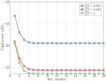
(a) $\sigma_{n}^{2}=-80\operatorname{dBm}$

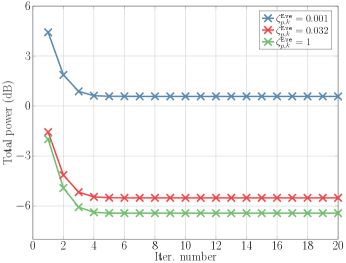
(b) $\sigma_{n}^{2}=-60\operatorname{dBm}$

Figure 2: Convergence behavior of the proposed secure FD ISAC algorithm for different SINR guarantees with $K=2$, $L=1$, and $P=1$. The noise powers for eavesdroppers and DL users are set equally to $\sigma_{\ell}^{2}=-80\operatorname{dBm}$ and $\sigma_{p}^{2}=-80\operatorname{dBm}$.

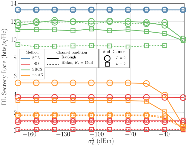
Figure 3: DL secrecy rate as a function of DL noise powers for different values of $L$, channel conditions, and methods. We set $\sigma_{n}^{2}=-80\operatorname{dBm}$ and $\sigma_{p}^{2}=-80\operatorname{dBm}$. The number of antennas is fixed to $N_{T}=N_{R}=12$. The Rician $K-$factor is referred to as $K_{r}$.

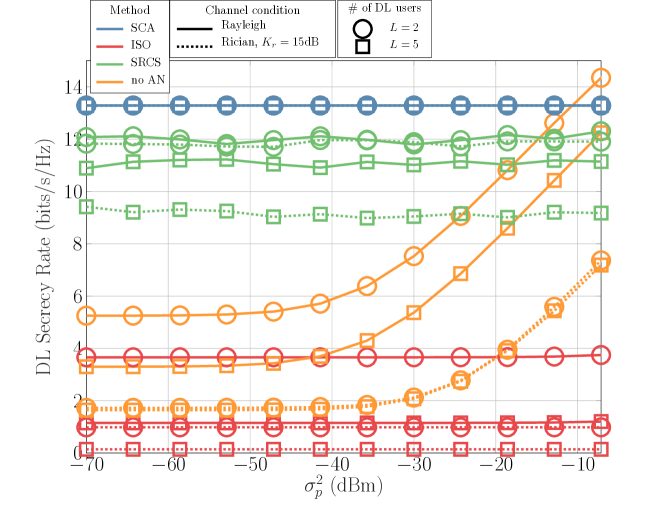
Figure 4: DL secrecy rate as a function of eavesdropper noise powers for different values of $L$, channel conditions, and methods. We set $\sigma_{n}^{2}=-80\operatorname{dBm}$ and $\sigma_{\ell}^{2}=-80\operatorname{dBm}$. The number of antennas is fixed to $N_{T}=N_{R}=12$.

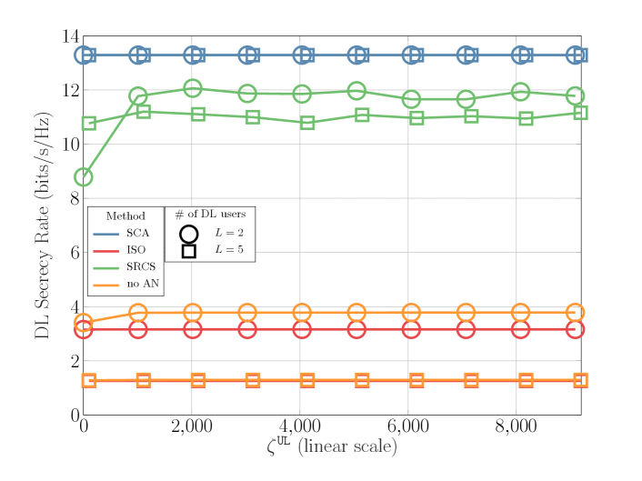
Figure 5: DL secrecy rate as a function of UL SINR requirement for different values of $L$ and methods. The simulation parameters are the same as Fig. 4. The channel distribution is Rayleigh.

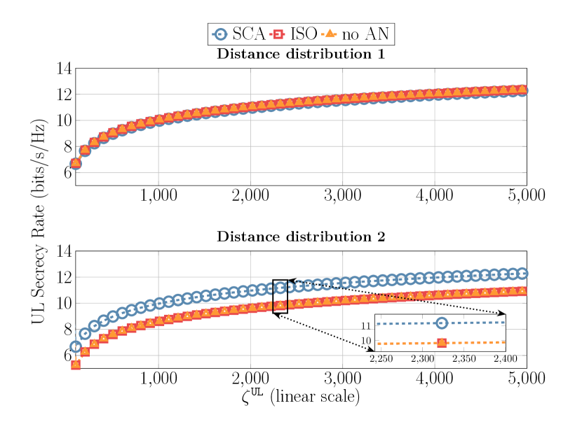
Figure 6: The UL secrecy rate behavior of different schemes for different position/distance distributions of the nodes. The noise powers are set to $\sigma_{n}^{2}=\sigma_{\ell}^{2}=\sigma_{p}^{2}=-80\operatorname{dBm}$. We fix $L=K=5$ legitimate users and $P=2$ eavesdroppers.

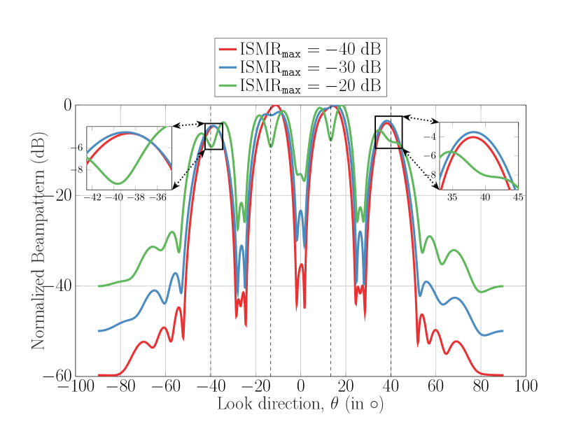
Figure 7: Beampatterns for different ISMR values for $P=4$ eavesdroppers. The noise powers are set to $\sigma_{n}^{2}=\sigma_{\ell}^{2}=\sigma_{p}^{2}=-80\operatorname{dBm}$. The number of transmit antennas is $N_{T}=16$. Vertical dashed lines correspond to eavesdroppers locations.

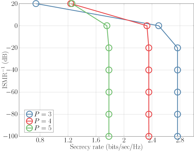
Figure 8: ISMR-secrecy tradeoff for different number of eavesdropping targets. The noise powers are set to $-80\operatorname{dBm}$. The number of antennas is $N_{T}=N_{R}=12$.

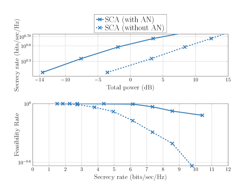
Figure 9: A comparison of the proposed scheme with and without AN. The number of transmit antennas is set to $N_{T}=12$. The noise powers are set to $\sigma_{n}^{2}=\sigma_{\ell}^{2}=\sigma_{p}^{2}=-80\operatorname{dBm}$.

V-A Parameter Setup

Unless otherwise stated, we use the simulation parameters depicted in Table I. Note that we have chosen the users and eavesdroppers to fall within the typical cell radius for mmWave communications, which is $500\operatorname{m}$ [48]. Monte Carlo type simulations have been performed in order to analyze the efficacy of the proposed secure ISAC beamforming and power allocation method. We consider perfect CSI of all nodes in the system, as the case of imperfect CSI is left out for future work. Moreover, the symbols are assumed to be i.i.d and independent from noise realizations. Furthermore, we use Rayleigh [49] and Rician distributions [50] to simulate different channel conditions, with log-normal shadowing of $20\operatorname{dB}$ and free space pathloss. The carrier frequency is centered around $28\operatorname{GHz}$. The transmit and receive array at the DFRC BS follow a ULA fashion, with $N_{T}=N_{R}=12$ antennas and inter-element spacing of $\frac{\lambda}{2}$. In addition, the transmit and receive antenna gains are $25\operatorname{dBi}$. The UL and DL users are equipped with single antennas with antenna gains of $17\operatorname{dBi}$ and $12\operatorname{dBi}$, respectively. The eavesdropper receive antenna gain is set at $12\operatorname{dBi}$. The thermal noise is set to $-174\operatorname{dBm/Hz}$. The residual SI is fixed at $-110\operatorname{dB}$. The DL user, eavesdropper, and UL user positions are set uniformly at $200\operatorname{m}$, $175\operatorname{m}$, and $150\operatorname{m}$, respectively. The DFRC BS transmit power is $40\operatorname{dBm}$.

TABLE I: Simulation Parameters

Parameter	Value
Number of cells	$1$
Cell radius	$200\operatorname{m}$
Transmit power by DFRC	$40\operatorname{dBm}$
DFRC transmit antenna gain	$25\operatorname{dBi}$
UL user antenna gain	$17\operatorname{dBi}$
DFRC receive antenna gain	$25\operatorname{dBi}$
DL receive antenna gain	$12\operatorname{dBi}$
Eavesdropper receive antenna gain	$12\operatorname{dBi}$
Carrier frequency	$28\operatorname{GHz}$
Thermal noise	$-174\operatorname{dBm/Hz}$
Shadowing	log-normal of $20\operatorname{dB}$
Pathloss exponent	$2$ (free space)
Residual SI	$-110\operatorname{dB}$
$N_{T}$, $N_{R}$	12
Antenna geometry	ULA
Antenna spacing	$\frac{\lambda}{2}$
Channel conditions	Rayleigh [49], Rician ($K_{r}=15\operatorname{dB}$) [50]
DL user positions	uniformly at $200\operatorname{m}$
Eavesdropper positions	uniformly at $175\operatorname{m}$
UL user positions	uniformly at $150\operatorname{m}$

V-B Benchmark Schemes

Throughout simulations, we compare our proposed method with the following three schemes:

• The isotropic design [51], denoted as ISO, is a widely used benchmark to show the performance through isotropic power allocation. In the FD case, the power is uniformly distributed across the UL, DL, and AN generation. In particular, we set $\boldsymbol{W}=\frac{P_{\tt{bud}}}{2}\frac{\mathcal{P}_{\boldsymbol{\boldsymbol{H}}_{r}}^{\perp}}{\|\mathcal{P}_{\boldsymbol{\boldsymbol{H}}_{r}}^{\perp}\|^{2}_{F}}$, where $\boldsymbol{\boldsymbol{H}}_{r}\in\mathbb{C}^{N_{T}\times L}$ contains all the DL channel vectors $\{\boldsymbol{h}_{r,\ell}\}_{\ell=1}^{L}$ stacked in the columns of $\boldsymbol{\boldsymbol{H}}_{r}$. This design ensures that legitimate users will not be subject to any interference, however, eavesdroppers’ reception may be harmed. On the other hand, the remaining available power is utilized for eigenbeamforming, i.e. $\boldsymbol{V}_{:,\ell}=\frac{\sqrt{P_{\tt{bud}}}}{\sqrt{2L}}\frac{\boldsymbol{h}_{r,\ell}}{\|\boldsymbol{h}_{r,\ell}\|}$.

• The no-AN design, denoted as no-AN, is intended for communication-only tasks, where zero forcing (ZF) precoding is performed, namely $\boldsymbol{V}=\boldsymbol{H}_{r}(\boldsymbol{H}_{r}^{H}\boldsymbol{H}_{r})^{-1}$ and $\boldsymbol{W}=\boldsymbol{0}$. Moreover, a uniform UL power allocation is given to UL users. This benchmark is indicating when the main focus should be oriented towards communications-only tasks.

• The secure ISAC design [25], denoted as SRCS, represents an optimized ISAC scheme where the optimization method aims at minimizing the signal-to-noise ratio (SNR) towards an eavesdropper, under a communication SINR constraint, a radar constraint and with a given power budget. Note that this method is only applicable for half-duplex communication scenarios.

• SCA without AN is another interesting benchmark, where we run Algorithm 1 by setting $\boldsymbol{W}=\boldsymbol{0}$, and by forming a sub-problem of $(\mathcal{P}_{1.3}^{(m)})$ where $\boldsymbol{W}$ is no longer treated as a variable simply because we set it to $\boldsymbol{0}$. This benchmark is intended to show the importance of AN.

The half-duplex scenario here is conducted with no UL communication users, and is dedicated only for DL secure communications, as well as sensing. Therefore, only DL ISAC tasks are modeled. This is a particular case of the FD ISAC model, i.e. by setting $K=0$. As the proposed method minimizes the power allocated for the secure FD ISAC system, we compute the total power consumed by the proposed method and use that power budget for all other benchmarks and settings, whether half-duplex or full-duplex, in order to have a fair comparison. Note that the power budget allocated to all the above three schemes is taken from the converged final output power of the proposed method. In other words, at each Monte Carlo trial, we first launch the proposed method, read the final power it had utilized, then pass that power budget to all the above three benchmarks to allow for a fair comparison. This is because the secrecy rate can be made arbitrarily large by increasing the transmission power. It is also worth noting that no-AN design and the isotropic AN are optimized for communications and secure communications, respectively. Therefore, no optimization is done regarding forming radar beams towards desired locations for further sensing processing at the DFRC BS.

V-C Simulation Results

Power Consumption

In Fig. 2a, we set $\sigma_{n}^{2}=-80\operatorname{dBm}$, which is a typical mmWave communication system thermal noise value [50] corresponding to a noise figure of $7\operatorname{dB}$, and a power spectral density (PSD) noise floor of $-174\operatorname{dBm/Hz}$. We also set $\sigma_{\ell}^{2}=-80\operatorname{dBm}$ and $\sigma_{p}^{2}=-80\operatorname{dBm}$ as typical noise variances for mmWave communication systems. Furthermore, we fix $K=2$ UL communication users, $L=1$ DL communication user and $P=1$ eavesdropper. In this simulation, we set $\zeta_{p,\tt{DFRC}}^{\tt{Eve}}=10^{-3}$, $\zeta_{\ell}^{\tt{DL}}=1,\forall\ell$ and $\zeta_{k}^{\tt{UL}}=1$. We run algorithm Algorithm 1 and average the obtained total consumed power per iteration over Monte Carlo trials. This simulation reveals how the total consumed power depends on the SINR requirements, as well as the noise variance at the DFRC BS. First of all, we highlight the power consumption as a function of secrecy requirements. More specifically, a more stringent constraint imposed on all the eavesdroppers has a direct impact on the total power consumption for a fixed noise power. Indeed, for a target SINR of $\zeta_{p,k}^{\tt{Eve}}=1$, we observe that the total consumed power settles at about $-26.36\operatorname{dB}$, whereas for a stricter SINR requirement of $\zeta_{p,k}^{\tt{Eve}}=0.032$, the total power converges to $-25.56\operatorname{dB}$, which is an additional $0.8\operatorname{dB}$. Furthermore, setting $\zeta_{p,k}^{\tt{Eve}}=0.001$, the total power converges to $-19.4\operatorname{dB}$, which is an additional $6.16\operatorname{dB}$.

Next, in Fig.2b, we increase the DFRC BS noise power to $\sigma_{n}^{2}=-60\operatorname{dBm}$, which can be attained by either increasing UL bandwidth, or at a high noise floor [52]. We also observe a similar trend regarding the SINR requirement as a function of total power consumed and convergence behaviour. For example, at $\zeta_{p,k}^{\tt{Eve}}=1$, the total consumed power stabilizes at $-6.43\operatorname{dB}$. Decreasing this SINR requirement to $0.032$ increases the total consumed power by $0.92$, i.e. $-5.51\operatorname{dB}$. Finally, a very strict SINR constraint on the eavesdroppers, $\zeta_{p,k}^{\tt{Eve}}=0.001$, consumes $0.58\operatorname{dB}$, which is an additional $6.1\operatorname{dB}$. Besides the SINR requirement, we also note that adding $20\operatorname{dB}$ of noise power is reflected within the total consumed power. For instance, setting $\zeta_{p,k}^{\tt{Eve}}=0.001$ at $\sigma_{n}^{2}=-80\operatorname{dBm}$ requires $20\operatorname{dB}$ less power than the same SINR requirement at $\sigma_{n}^{2}=-60\operatorname{dBm}$. It is also worth noting that the algorithm converges in about $20$ iterations.

DL Secrecy Behaviour

In Fig. 3, the DL secrecy rate is analyzed as a function of $\sigma_{\ell}^{2}$. We set a total of $P=2$ eavesdroppers and $K=9$ legitimate UL users. The number of antennas is fixed to $N_{T}=N_{R}=12$. We have fixed the SINR requirements at $\zeta_{\ell}^{\tt{DL}}=\zeta_{k}^{\tt{UL}}=10^{4}$ and $\zeta_{p,\tt{DFRC}}^{\tt{Eve}}=\zeta_{p,\tt{DFRC}}^{\tt{Eve}}=10^{-5}$, for all $\ell,k,p$. We set $\sigma_{n}^{2}=-80\operatorname{dBm}$ and $\sigma_{p}^{2}=-80\operatorname{dBm}$. It is observed that, regardless of channel conditions, the proposed method settles at about $13.28\operatorname{bits/sec/Hz}$, which is inferred directly from the SINR requirements, i.e. $\log_{2}(1+10^{4})-\log_{2}(1+10^{-5})$. This reveals the consistency of our method regardless of the operating noise power level. The optimized SRCS method is somewhat stable as the DL secrecy rate fluctuates around $11.9\operatorname{bits/sec/Hz}$ for $L=2$ for all channel conditions. As the number of DL users increases, the secrecy rate decreases to around $10.98\operatorname{bits/sec/Hz}$ for Rayleigh channels and $9.31\operatorname{bits/sec/Hz}$ for Rician channel with $15\operatorname{dB}$ Rician factor [50]. This loss compared to the proposed method can be explained by the fact that SRCS is optimized to minimize the eavesdropper SNR towards a given direction and under a power budget constraint. Furthermore, the isotropic method is also stable as, for Rayleigh channels, it attains $3.66\operatorname{bits/sec/Hz}$ for $L=2$ and $0.98\operatorname{bits/sec/Hz}$ for Rician channels with $K_{\tt{r}}=15\operatorname{dB}$. The secrecy rate decreases with increasing $L$ as a drop of $2.51\operatorname{bits/sec/Hz}$ is observed for $L=2$ in case of Rayleigh channels and a drop of $0.84\operatorname{bits/sec/Hz}$ in case of Rician channels. Moreover, the no-AN method depicts a different behavior. More specifically, in cases of high DL SNR, i.e. low $\sigma_{\ell}^{2}$, the no-AN is generally better than the isotropic allocation, as for Rayleigh channels, a $5.2\operatorname{bits/sec/Hz}$ secrecy is attained for $L=2$, and $3.2\operatorname{bits/sec/Hz}$ for $L=5$, whereas secrecy rates of $1.72\operatorname{bits/sec/Hz}$ ($L=2$) and $1.63\operatorname{bits/sec/Hz}$ ($L=5$) is achieved for Rician channels. In the low SNR regime, $\sigma_{\ell}^{2}>-55\operatorname{dBm}$, we see that the DL secrecy rate for no AN decays to zero, as expected. This is because the power is not optimally distributed, and hence the SINR at the eavesdroppers will exceed that of the legitimate users after a certain $\sigma_{\ell}^{2}$. In addition, we highlight two main insights: First, the proposed method performs better than the isotropic and the no-AN methods due to the fact power and beamfomers are optimized to achieve target secrecy rates under minimal power. Second, we interestingly observe that strong LoS channels may be harmful for the secrecy rates, as higher channel correlations are achieved, which can deteriorate the overall secrecy performance.

In Fig. 4, we study the DL secrecy rate performance as a function of noise power at the eavesdroppers. We set the same simulation parameters as those in Fig. 3. A similar trend is noticed for all the methods, except for the no AN case. In particular, when the noise at the eavesdroppers exceeds $-30\operatorname{dBm}$, the DL secrecy rate for the no AN case increases and can outperform the DL secrecy rate of the proposed method. This can be explained by the fact that the scheme without AN utilizes all the available power to optimize the communication performance, without having to worry about the eavesdroppers, which are already experiencing high noise power levels. Therefore, in such a noisy regime, it may be enough to focus on maximizing the DL SINR without allocating power towards AN beamforming. Another point to highlight is that the proposed SCA is optimized to target a minimum acceptable DL SINR regardless of the noise level $\sigma_{p}^{2}$, therefore, in order to achieve a higher secrecy rate, we would have to increase $\rho^{\tt{DL}}$, similar to the simulations corresponding to Fig. 6. SRCS, as well as the proposed method, seek to attain the required SINR values as part of the optimization procedure, whereas the no AN performs ZF precoding and can attain better performance only when the eavesdroppers operate at a high noise power level.

In Fig. 5, our goal is to study the influence of UL SINR requirements on the DL secrecy rate. We fix the same simulation parameters as in Fig. 4. This simulation shows how the UL SINR requirement impacts the DL secrecy rate. The SRCS method, being half-duplex, will profit from all the power spent to improve its DL secrecy rate. But, as observed, the SRCS method settles around $11.96\operatorname{bits/sec/Hz}$ for $L=2$ and $11.07\operatorname{bits/sec/Hz}$ for $L=5$, whereas the proposed method supplies a stable DL secrecy rate of $13.28\operatorname{bits/sec/Hz}$, for any given UL SINR requirement. It is also observed that with increasing number of DL users, all but the proposed method deteriorate in terms of secrecy rate. The DL secrecy rate achieved by the no-AN design method increases with increasing $\rho^{\tt{UL}}$ since more power is being allocated to the system. However, the DL secrecy rate attained by no AN scheme depends on the number of legitimate UL and DL communication users. Generally speaking, the lower $L$ is, the higher the DL secrecy rate that can be achieved.

UL Secrecy behaviour

In Fig. 6, we study the UL secrecy rate behavior versus the SINR requirement on the UL, i.e. $\rho^{\tt{UL}}$. We distinguish two distance/position distributions, where the UL users are placed on a circle of radius $150\operatorname{m}$ for the first distribution, whereas the same UL users are placed on a straight line uniformly distributed on $[1,500]\operatorname{m}$. In the first distribution, the performance of all three methods perform alike, as a uniform power allocation onto the UL users suffices to achieve a desired SINR on the UL users. In the second distribution, however, for the same total consumed power, the proposed SCA method can achieve a better UL secrecy rate, i.e. an additional $1.38\operatorname{bits/sec/Hz}$, as the no-AN and isotropic schemes allocate equal amounts of power to all the UL users. Note that the SRCS method is not present because it is dedicated for half-duplex ISAC communication systems.

ISMR impact on Beampattern Design

In Fig. 7, we study the resulting normalized beampattern after executing Algorithm 1 for different ISMR values. The normalized beampattern is defined as

$$P(\theta)=\frac{\boldsymbol{a}^{H}(\theta)\widehat{\boldsymbol{R}}_{\boldsymbol{x}\boldsymbol{x}}\boldsymbol{a}(\theta)}{\max_{\theta}\boldsymbol{a}^{H}(\theta)\widehat{\boldsymbol{R}}_{\boldsymbol{x}\boldsymbol{x}}\boldsymbol{a}(\theta)},$$ (47)

where $\widehat{\boldsymbol{R}}_{\boldsymbol{x}\boldsymbol{x}}=\widehat{\boldsymbol{V}}\widehat{\boldsymbol{V}}^{H}+\widehat{\boldsymbol{W}}$. We evaluate $P(\theta)$ for different values of $\theta$ in order to obtain the beampattern. For the SINR requirements on the legitimate users, we set $\zeta_{k}^{\tt{UL}}=\zeta_{\ell}^{\tt{DL}}=10^{2}$. As for the DL/UL SINR on evesdroppers, we fix $\zeta_{p,k}^{\tt{Eve}}=\zeta_{p,\tt{DFRC}}^{\tt{Eve}}=0.1$. We also set all noise powers to $-80\operatorname{dBm}$. This simulation shows how the $\operatorname{ISMR}_{\tt{max}}$ can help control the mainlobe to sidelobe ratio power. Indeed, when setting $\operatorname{ISMR}_{\tt{max}}=-30\operatorname{dB}$, we observe that the sidelobe power is roughly $10\operatorname{dB}$ more than the beampattern corresponding to that of $\operatorname{ISMR}_{\tt{max}}=-20\operatorname{dB}$ and $10\operatorname{dB}$ less than that of $\operatorname{ISMR}_{\tt{max}}=-40\operatorname{dB}$. It is worth noting that a less strict ISMR constraint, allows for a higher achievable secrecy, which will be clarified in the next simulation.

Sensing-Secrecy ISAC Trade-off

In Fig. 8, we study the sensing-secrecy trade-off, where the achievable ISMR inverse is plotted against the secrecy rate. All noise powers are set to a level of $-80\operatorname{dBm}$, and the number of antennas is set to $N_{T}=N_{R}=12$. It is revealed that the secrecy rate improves on the expense of increasing the ISMR. Studying the trade-off at extreme cases for $P=3$, we observe that an $\operatorname{ISMR}^{-1}$ can only achieve a secrecy rate of $0.74\operatorname{bits/sec/Hz}$, which is the case of pointy beams where the echo return experiences a power boost good clutter rejection properties, whereas relaxing the $\operatorname{ISMR}^{-1}$ anywhere below $-20\operatorname{dB}$ can achieve a secrecy rate of $2.76\operatorname{bits/sec/Hz}$. Increasing the number of eavesdroppers impacts the tradeoffs, as lower secrecy rates are achieved via the same resources. For instance, an additional evesdropper lowers the secrecy rate to $2.35\operatorname{bits/sec/Hz}$ when $\operatorname{ISMR}^{-1}\leq-20\operatorname{dB}$. We conclude that the $\operatorname{ISMR}_{\tt{max}}$ can also allow us to achieve favorable tradeoffs to attain a desired secrecy rate, while performing radar tasks.

Importance of AN

In Fig. 9, we study the performance of the proposed method with and without AN. In the first subplot of Fig. 9, we study the secrecy rate as a function of total consumed power. We can observe a significant gain in terms of total consumed power for nearly all secrecy rates. For example, a target secrecy rate of $3.79\operatorname{bits/sec/Hz}$ requires $8.35\operatorname{dB}$ without using AN, whereas the same secrecy rate consumes only $-1.92\operatorname{dB}$ for the proposed method with AN, which translates to a total power gain of about $10.27\operatorname{dB}$. This can be explained through the additional subspace created by the AN, which can indeed save notable amounts of power to achieve a desired secrecy rate.

In the second subplot of Fig. 9, we study the feasibility rate of both schemes, which is defined as [43]

$$\operatorname{feasibility\ rate}=\frac{\#\text{ of feasible solutions}}{\#\text{ of cases}}.$$ (48)

It is observed that for secrecy rate below $2.73\operatorname{bits/sec/Hz}$, the feasibility rate of both schemes is nearly $1$, i.e. we can always find beamformers and power values (as well as AN covariance matrix for the scheme with AN) to target the desired secrecy rates. When the secrecy rate goes beyond $2.73\operatorname{bits/sec/Hz}$, we can see that the proposed scheme with AN outperforms that without AN. For instance, for a fixed desired feasibility rate of $0.93$, i.e. a feasible solution can be found $93\%$ of the time, the proposed scheme without AN can only achieve a secrecy rate up to $3.79\operatorname{bits/sec/Hz}$, whereas the proposed scheme with AN can nearly double that secrecy rate to go up to $7.35\operatorname{bits/sec/Hz}$. This is due to the additional degrees of freedom introduced by the AN, which enables us to achieve much higher secrecy rates for more cases.

VI Conclusions and Research Directions

We have provided a FD ISAC system model, where a unified waveform for sensing and secure communications is transmitted in the DL to maintain desired UL and DL secrecy rate performance, whilst guaranteeing desired ISMR radar levels. Under the proposed model, we proposed a power efficient ISAC optimization framework to jointly satisfy UL/DL secrecy rates, under a maximal acceptable ISMR, which further aids the DFRC BS at probing sensing information from the eavesdroppers. The total power minimization problem is intended to economize the overall transmitted UL/DL power and the artificial noise generation power. Due to the intractability introduced by the non-convex problem, we propose iterating via successive convex approximations, which is deemed suitable due to the low number of iterations spent by the method, and its capability in simultaneously guaranteeing UL/DL secrecy rates and ISMR levels. Our results support the effectiveness of the method, as compared to classical secure beamforming approaches and secure ISAC methods. Future work include extensions towards an energy-efficient optimization problem that can also be formulated under the proposed FD ISAC system model. Indeed, energy efficiency emanated as a crucial key performance indicator for the deployment of sustainable and green wireless networks [53]. Furthermore, an extension to the imperfect CSI case will also be part of our future work.

In addition to the security vulnerabilities in future wireless communications mentioned in this paper, the survey in [54] highlights a number of critical problems over beyond 5G (B5G) wireless networks and internet of things (IoT). For instance, edge networks face an onslaught of risks and attacks because of their limited processing power, memory capacity, battery life, and network bandwidth, in addition to threats encountered in IoT, such as impersonation attacks and routing attacks. As highlighted by [54], and references therein, DL-based techniques seem to be a promising approach for future wireless communications, e.g., physical-layer authentication [55]. In some cases, however, learning can be effective for online usage due to its low online complexity, but it can suffer from high computational complexity when training, whereas a fully distributed training approach can suffer from convergence issues due to the partial availability of state information for training. In contrast to a centralized and insecure training approach for wireless communications, edge learning (EL) has been proposed to distribute the implementation of maximum likelihood (ML) algorithms over multiple edge devices, thereby reducing computational complexity and malicious attacks. Furthermore, the use of EL methods in a range of future communication systems, including B5G wireless networks, is also being considered. For instance, [56] aims at communications and privacy protection via federated learning (FL), whereas [57] detects network intrusion. As future work, we can leverage the philosophy of EL in order to distribute the computations of the proposed SCA-based algorithm for minimal power transmissions in secure FD ISAC, which can contribute to lower computations due to the relatively large number of required iterations.

Appendix A Rank-1 Optimality

We start by expressing the Lagrangian function of the optimization problem given at iteration $m$ in (46). It can be expressed as

$$\begin{split}&\mathcal{L}(\boldsymbol{V}_{1}\ldots\boldsymbol{V}_{L},\boldsymbol{W},\boldsymbol{p},\boldsymbol{a},\boldsymbol{b},\boldsymbol{c},\boldsymbol{d},\zeta,\boldsymbol{\Pi}_{0}\ldots\boldsymbol{\Pi}_{L},\boldsymbol{\pi})\\ &=-\sum\limits_{\ell=1}^{L}\operatorname{tr}(\boldsymbol{\boldsymbol{V}}_{\ell})-\operatorname{tr}(\boldsymbol{W})-\boldsymbol{1}^{T}\boldsymbol{p}+\operatorname{tr}(\boldsymbol{\Pi}_{0}\boldsymbol{W})+\sum\limits_{\ell=1}^{L}\operatorname{tr}(\boldsymbol{\Pi}_{\ell}\boldsymbol{V}_{\ell})\\ &+\boldsymbol{\pi}^{T}\boldsymbol{p}+\sum\nolimits_{\ell=1}^{L}a_{\ell}\phi_{1,\ell}+\sum\nolimits_{k=1}^{K}b_{k}\phi_{2,k}+\sum\nolimits_{p=1}^{P}c_{p}\phi_{3,p}\\ &+\sum\nolimits_{p=1}^{P}\sum\nolimits_{k=1}^{K}d_{p,k}\phi_{4,p,k}+\zeta\phi_{5},\end{split}$$

where the Lagrangian dual variables satisfy $a_{\ell}\geq 0,b_{k}\geq 0,c_{p}\geq 0,d_{p,k}\geq 0,\zeta\geq 0,\boldsymbol{\Pi}_{\ell}\succeq\boldsymbol{0}$ for all $\ell,k,p$. The functions $\phi_{1,\ell},\phi_{2,k},\phi_{3,p},\phi_{4,p,k},\phi_{5}$ are obtained by mapping the constraints in (46) under the form $\phi\geq 0$. Due to compact representation, we have omitted the dependence of $\phi$ on the optimization variables and the iteration number $m$. To this extent, we can now define the Lagrange dual function is then defined as follows

$$\begin{split}&g(\boldsymbol{a},\boldsymbol{b},\boldsymbol{c},\boldsymbol{d},\zeta,\boldsymbol{\Pi}_{0}\ldots\boldsymbol{\Pi}_{L},\boldsymbol{\pi})\\ &=\max\limits_{\mathcal{S}}\mathcal{L}(\boldsymbol{V}_{1}\ldots\boldsymbol{V}_{L},\boldsymbol{W},\boldsymbol{p},\boldsymbol{a},\boldsymbol{b},\boldsymbol{c},\boldsymbol{d},\zeta,\boldsymbol{\Pi}_{0}\ldots\boldsymbol{\Pi}_{L},\boldsymbol{\pi}),\end{split}$$ (49)

where the set $\mathcal{S}$ is defined as $\mathcal{S}=\{\boldsymbol{V}_{\ell}\succeq\boldsymbol{0},\boldsymbol{W}\succeq\boldsymbol{0},\boldsymbol{p}\geq\boldsymbol{0}\}$. But since problem $(\mathcal{P}_{1.3}^{(m)})$ is a convex optimization problem with zero duality gap, we can solve the problem via its dual

$$(\mathcal{D}):\min\limits_{\bar{\mathcal{S}}}g(\boldsymbol{a},\boldsymbol{b},\boldsymbol{c},\boldsymbol{d},\zeta,\boldsymbol{\Pi}_{0}\ldots\boldsymbol{\Pi}_{L},\boldsymbol{\pi}),$$ (50)

where $\bar{\mathcal{S}}=\{\zeta\geq 0,\boldsymbol{a},\boldsymbol{b},\boldsymbol{c},\boldsymbol{d},\boldsymbol{\pi}\succeq 0,\boldsymbol{\Pi}_{\ell}\succeq 0,\forall\ell\}$. Let the optimal solution of problem $(\mathcal{D})$ as $\boldsymbol{a}^{\operatorname{opt}},\boldsymbol{b}^{\operatorname{opt}},\boldsymbol{c}^{\operatorname{opt}},\boldsymbol{d}^{\operatorname{opt}},\zeta^{\operatorname{opt}},\boldsymbol{\Pi}_{0}^{\operatorname{opt}}\ldots\boldsymbol{\Pi}_{L}^{\operatorname{opt}},\boldsymbol{\pi}^{\operatorname{opt}}$. This means that the optimal $\ell^{th}$ DL beamforming matrix, the AN covariance matrix, and UL power allocation denoted as $\boldsymbol{V}_{\ell}^{\operatorname{opt}},\boldsymbol{W}^{\operatorname{opt}},\boldsymbol{p}^{\operatorname{opt}}$ also maximizes $\mathcal{L}(\boldsymbol{V}_{1}\ldots\boldsymbol{V}_{L},\boldsymbol{W},\boldsymbol{p},\boldsymbol{a}^{\operatorname{opt}}\ldots\boldsymbol{\pi}^{\operatorname{opt}})$, which means that we can find the optimal solution $\boldsymbol{V}_{\ell}^{\operatorname{opt}}$ by solving the following optimization problem

$$\begin{split}\max\limits_{\boldsymbol{V}_{\ell}\succeq\boldsymbol{0}}\Bigg{\{}&-\operatorname{tr}(\boldsymbol{V}_{\ell})+\frac{a_{\ell}}{\zeta_{\ell}^{\tt{DL}}}\operatorname{tr}(\boldsymbol{V}_{\ell}\boldsymbol{H}_{r,\ell})+\operatorname{tr}(\boldsymbol{\Pi}_{\ell}\boldsymbol{V}_{\ell})\\ &-\sum\nolimits_{k=1}^{K}b_{k}\boldsymbol{h}^{H}_{t,k}[\boldsymbol{\Phi}_{k}^{(m)}]^{-1}\boldsymbol{C}\boldsymbol{V}_{\ell}\boldsymbol{C}^{H}[\boldsymbol{\Phi}_{k}^{(m)}]^{-1}\boldsymbol{h}_{t,k}\\ &-\sum\limits_{p=1}^{P}\big{(}\frac{c_{p}|\alpha_{p}|^{2}}{\zeta_{p,\tt{DFRC}}^{\tt{Eve}}}-\sum\limits_{k=1}^{K}d_{p,k}|\alpha_{p}|^{2}\big{)}\boldsymbol{a}_{N_{T}}^{H}(\theta_{p})\boldsymbol{V}_{\ell}\boldsymbol{a}_{N_{T}}(\theta_{p})\\ &\end{split}{}$$ (51)

where terms that are independent of $\boldsymbol{V}_{\ell}$ are ignored. We can compactly express (51) as follows

$$\max\limits_{\boldsymbol{V}_{\ell}\succeq\boldsymbol{0}}\operatorname{tr}(\Phi\boldsymbol{V}_{\ell})-\operatorname{tr}\Big{\{}(\boldsymbol{I}+\boldsymbol{\Gamma}+\zeta^{\operatorname{opt}}\boldsymbol{A}_{s})\boldsymbol{V}_{\ell}\Big{\}},$$ (52)

where

$$\Phi =\frac{a_{\ell}^{\operatorname{opt}}}{\zeta_{\ell}^{\tt{DL}}}\boldsymbol{H}_{r,\ell}+\boldsymbol{\Upsilon}+\zeta^{\operatorname{opt}}\operatorname{ISMR}_{\tt{max}}\boldsymbol{A}_{m}+\boldsymbol{\Pi}_{\ell}^{\operatorname{opt}},$$ (53)

$$\boldsymbol{\Upsilon} =\sum\nolimits_{p=1}^{P}\sum\nolimits_{k=1}^{K}d_{p,k}^{\operatorname{opt}}|\alpha_{p}|^{2}\boldsymbol{a}_{N_{T}}(\theta_{p})\boldsymbol{a}_{N_{T}}^{H}(\theta_{p}),$$ (54)

Note that (52) is bounded above because both $\Phi$ and $\boldsymbol{I}+\boldsymbol{\Gamma}+\zeta^{\operatorname{opt}}\boldsymbol{A}_{s}$ are positive semi-definite. Now, since $\boldsymbol{I}+\boldsymbol{\Gamma}+\zeta^{\operatorname{opt}}\boldsymbol{A}_{s}\succeq\boldsymbol{0}$, there is a unique Hermitian positive definite matrix $\boldsymbol{R}_{k}^{\frac{1}{2}}$, such that $\boldsymbol{I}+\boldsymbol{\Gamma}+\zeta^{\operatorname{opt}}\boldsymbol{A}_{s}=\boldsymbol{R}^{\frac{1}{2}}\boldsymbol{R}^{\frac{1}{2}}$ [58]. Using square root matrix decomposition, we can write our cost in (52) as

$$\max\limits_{\widetilde{\boldsymbol{V}}_{\ell}\succeq\boldsymbol{0}}\operatorname{tr}\Big{\{}\boldsymbol{R}^{-\frac{1}{2}}\Phi\boldsymbol{R}^{-\frac{1}{2}}\widetilde{\boldsymbol{V}}_{\ell}\Big{\}}-\operatorname{tr}\Big{\{}\widetilde{\boldsymbol{V}}_{\ell}\Big{\}},$$ (55)

where $\widetilde{\boldsymbol{V}}_{\ell}=\boldsymbol{R}^{\frac{1}{2}}\boldsymbol{V}_{\ell}\boldsymbol{R}^{\frac{1}{2}}$. Now, suppose that the optimal solution, denoted hereby as $\widetilde{\boldsymbol{V}}_{\ell}^{\operatorname{opt}}$, is not $\operatorname{rank}$-one, i.e. $\operatorname{rank}$ $S>1$. Then, employing the eigenvalue decomposition, we have that $\widetilde{\boldsymbol{V}}_{\ell}^{\operatorname{opt}}=\sum\nolimits_{n=1}^{S}\beta_{n}\widetilde{\boldsymbol{v}}_{n}\widetilde{\boldsymbol{v}}_{n}^{H}$ where $\beta_{n}\geq 0$ and $\|\widetilde{\boldsymbol{v}}_{n}\|=1$, the cost in (55) can be written as

$$\max\limits_{\|\widetilde{\boldsymbol{v}}_{n}\|=1,\beta_{n}\geq 0}\sum\nolimits_{n=1}^{S}\beta_{n}\big{(}\|\Phi^{\frac{1}{2}}\boldsymbol{R}^{-\frac{1}{2}}\widetilde{\boldsymbol{v}}_{n}\|^{2}-1\big{)}.$$ (56)

Notice that the cost in (56) is upper-bounded as follows

$$\begin{split}&\sum\limits_{n=1}^{S}\beta_{n}\big{(}\|\Phi^{\frac{1}{2}}\boldsymbol{R}^{-\frac{1}{2}}\widetilde{\boldsymbol{v}}_{n}\|^{2}-1\big{)}\leq\sum\limits_{n=1}^{S}\beta_{n}\big{(}\|\Phi^{\frac{1}{2}}\boldsymbol{R}^{-\frac{1}{2}}\widetilde{\boldsymbol{v}}_{\hat{n}}\|^{2}-1\big{)},\end{split}$$

where $\Phi^{\frac{1}{2}}$ is the square root decomposition of $\Phi$. Indeed, we have upper bounded all terms of the form $\|\Phi^{\frac{1}{2}}\boldsymbol{R}^{-\frac{1}{2}}\widetilde{\boldsymbol{v}}_{n}\|^{2}$ by $\|\Phi^{\frac{1}{2}}\boldsymbol{R}^{-\frac{1}{2}}\widetilde{\boldsymbol{v}}_{\hat{n}}\|^{2}$ where $\hat{n}=\operatorname*{arg\,max}\nolimits_{n=1\ldots S}\|\Phi^{\frac{1}{2}}\boldsymbol{R}^{-\frac{1}{2}}\widetilde{\boldsymbol{v}}_{n}\|^{2}$. But, this bound is achieved by the following $\operatorname{rank}$-one form $\widetilde{\boldsymbol{V}}_{\ell}^{\operatorname{rank}-1}=(\sum\nolimits_{n=1}^{S}\beta_{n})\widetilde{\boldsymbol{v}}_{\hat{n}}\widetilde{\boldsymbol{v}}_{\hat{n}}^{H}$, which is a contradiction of the assumption that $S>1$. Therefore, $\widetilde{\boldsymbol{V}}_{\ell}^{\operatorname{opt}}$ has to be $\operatorname{rank}$-1 optimal. Now, since we have ${\boldsymbol{V}}_{\ell}^{\operatorname{opt}}=\boldsymbol{R}^{-\frac{1}{2}}\widetilde{\boldsymbol{V}}_{\ell}^{\operatorname{opt}}\boldsymbol{R}^{-\frac{1}{2}}$, we must also have that ${\boldsymbol{V}}_{\ell}^{\operatorname{opt}}$ is $\operatorname{rank}$-one optimal according to $\operatorname{rank}(\boldsymbol{A}\boldsymbol{B})\leq\min\{\operatorname{rank}(\boldsymbol{A}),\operatorname{rank}(\boldsymbol{B})\}$, which finalizes the proof.

References

- [1] M. Chafii, L. Bariah, S. Muhaidat, and M. Debbah, “Twelve Scientific Challenges for 6G: Rethinking the Foundations of Communications Theory,” IEEE Communications Surveys & Tutorials, vol. 25, no. 2, pp. 868–904, 2023.
- [2] C. W. Dukes, “Committee on National Security Systems (CNSS) Glossary, CNSSI No. 4009,” DoD Ft Meade, 2015.
- [3] S. L. Garfinkel, “Draft (2nd) NIST SP 800-188, De-Identification of Government Datasets,” 2016.
- [4] M. Li, Y. Meng, J. Liu, H. Zhu, X. Liang, Y. Liu, and N. Ruan, “When CSI meets public WiFi: inferring your mobile phone password via WiFi signals,” in Proceedings of the 2016 ACM SIGSAC conference on computer and communications security, 2016, pp. 1068–1079.
- [5] A. Chorti, A. N. Barreto, S. Köpsell, M. Zoli, M. Chafii, P. Sehier, G. Fettweis, and H. V. Poor, “Context-Aware Security for 6G Wireless: The Role of Physical Layer Security,” IEEE Communications Standards Magazine, vol. 6, no. 1, pp. 102–108, 2022.
- [6] Y. Meng, J. Li, H. Zhu, X. Liang, Y. Liu, and N. Ruan, “Revealing Your Mobile Password via WiFi Signals: Attacks and Countermeasures,” IEEE Transactions on Mobile Computing, vol. 19, no. 2, pp. 432–449, 2020.
- [7] X. Jiao, M. Mehari, W. Liu, M. Aslam, and I. Moerman, “Openwifi CSI fuzzer for authorized sensing and covert channels,” in Proceedings of the 14th ACM Conference on Security and Privacy in Wireless and Mobile Networks, 2021, pp. 377–379.
- [8] J. M. Hamamreh, H. M. Furqan, and H. Arslan, “Classifications and Applications of Physical Layer Security Techniques for Confidentiality: A Comprehensive Survey,” IEEE Communications Surveys & Tutorials, vol. 21, no. 2, pp. 1773–1828, 2019.
- [9] S. Goel and R. Negi, “Guaranteeing Secrecy using Artificial Noise,” IEEE Transactions on Wireless Communications, vol. 7, no. 6, pp. 2180–2189, 2008.
- [10] H.-M. Wang, J. Bai, and L. Dong, “Intelligent Reflecting Surfaces Assisted Secure Transmission Without Eavesdropper’s CSI,” IEEE Signal Processing Letters, vol. 27, pp. 1300–1304, 2020.
- [11] M. Pei, J. Wei, K.-K. Wong, and X. Wang, “Masked Beamforming for Multiuser MIMO Wiretap Channels with Imperfect CSI,” IEEE Transactions on Wireless Communications, vol. 11, no. 2, pp. 544–549, 2012.
- [12] P. Zhao, M. Zhang, H. Yu, H. Luo, and W. Chen, “Beamforming design of sum secrecy rate optimization for MU-MISO channel under sum power constraint,” in 2014 Sixth International Conference on Wireless Communications and Signal Processing (WCSP), 2014, pp. 1–6.
- [13] H.-M. Wang, M. Luo, Q. Yin, and X.-G. Xia, “Hybrid Cooperative Beamforming and Jamming for Physical-Layer Security of Two-Way Relay Networks,” IEEE Transactions on Information Forensics and Security, vol. 8, no. 12, pp. 2007–2020, 2013.
- [14] Z. Lin, K. An, H. Niu, Y. Hu, S. Chatzinotas, G. Zheng, and J. Wang, “SLNR-Based Secure Energy Efficient Beamforming in Multibeam Satellite Systems,” IEEE Transactions on Aerospace and Electronic Systems, vol. 59, no. 2, pp. 2085–2088, 2023.
- [15] Q. Li, H. Song, and K. Huang, “Achieving Secure Transmission with Equivalent Multiplicative Noise in MISO Wiretap Channels,” IEEE Communications Letters, vol. 17, no. 5, pp. 892–895, 2013.
- [16] L. Zhai, Y. Zou, J. Zhu, and B. Li, “Improving Physical Layer Security in IRS-Aided WPCN Multicast Systems via Stackelberg Game,” IEEE Transactions on Communications, vol. 70, no. 3, pp. 1957–1970, 2022.
- [17] M. Wijewardena, T. Samarasinghe, K. T. Hemachandra, S. Atapattu, and J. S. Evans, “Physical Layer Security for Intelligent Reflecting Surface Assisted Two–Way Communications,” IEEE Communications Letters, vol. 25, no. 7, pp. 2156–2160, 2021.
- [18] Y. Qi and M. Vaezi, “IRS-Assisted Physical Layer Security in MIMO-NOMA Networks,” IEEE Communications Letters, vol. 27, no. 3, pp. 792–796, 2023.
- [19] Y. Guo, Y. Liu, Q. Wu, Q. Shi, and Y. Zhao, “Enhanced Secure Communication via Novel Double-Faced Active RIS,” IEEE Transactions on Communications, vol. 71, no. 6, pp. 3497–3512, 2023.
- [20] W. Wang, Y. Cao, M. Sheng, J. Tang, N. Zhao, D. Niyato, and K.-K. Wong, “Secure Beamforming for IRS-Enhanced NOMA Networks,” IEEE Wireless Communications, vol. 30, no. 1, pp. 134–140, 2023.
- [21] A. Nooraiepour and T. M. Duman, “Randomized Serially Concatenated LDGM Codes for the Gaussian Wiretap Channel,” IEEE Communications Letters, vol. 22, no. 4, pp. 680–683, 2018.
- [22] D. Klinc, J. Ha, S. W. McLaughlin, J. Barros, and B.-J. Kwak, “LDPC Codes for the Gaussian Wiretap Channel,” IEEE Transactions on Information Forensics and Security, vol. 6, no. 3, pp. 532–540, 2011.
- [23] R. A. Chou, M. R. Bloch, and E. Abbe, “Polar Coding for Secret-Key Generation,” IEEE Transactions on Information Theory, vol. 61, no. 11, pp. 6213–6237, 2015.
- [24] Y. Zhang, A. Liu, C. Gong, G. Yang, and S. Yang, “Polar-LDPC Concatenated Coding for the AWGN Wiretap Channel,” IEEE Communications Letters, vol. 18, no. 10, pp. 1683–1686, 2014.
- [25] N. Su, F. Liu, and C. Masouros, “Secure Radar-Communication Systems With Malicious Targets: Integrating Radar, Communications and Jamming Functionalities,” IEEE Transactions on Wireless Communications, vol. 20, no. 1, pp. 83–95, 2021.
- [26] Z. Yang, D. Li, N. Zhao, Z. Wu, Y. Li, and D. Niyato, “Secure Precoding Optimization for NOMA-Aided Integrated Sensing and Communication,” IEEE Transactions on Communications, vol. 70, no. 12, pp. 8370–8382, 2022.
- [27] D. Li, Z. Yang, N. Zhao, Z. Wu, Y. Li, and D. Niyato, “Joint Precoding and Jamming Design for Secure Transmission in NOMA-ISAC Networks,” in 2022 14th International Conference on Wireless Communications and Signal Processing (WCSP), 2022, pp. 764–769.
- [28] Z. He, W. Xu, H. Shen, D. W. K. Ng, Y. C. Eldar, and X. You, “Full-Duplex Communication for ISAC: Joint Beamforming and Power Optimization,” IEEE Journal on Selected Areas in Communications, vol. 41, no. 9, pp. 2920–2936, 2023.
- [29] Z. Liu, S. Aditya, H. Li, and B. Clerckx, “Joint Transmit and Receive Beamforming Design in Full-Duplex Integrated Sensing and Communications,” IEEE Journal on Selected Areas in Communications, vol. 41, no. 9, pp. 2907–2919, 2023.
- [30] L. Zhao, D. W. K. Ng, and J. Yuan, “Multi-User Precoding and Channel Estimation for Hybrid Millimeter Wave Systems,” IEEE Journal on Selected Areas in Communications, vol. 35, no. 7, pp. 1576–1590, 2017.
- [31] Z. Lyu, G. Zhu, and J. Xu, “Joint Maneuver and Beamforming Design for UAV-Enabled Integrated Sensing and Communication,” IEEE Transactions on Wireless Communications, vol. 22, no. 4, pp. 2424–2440, 2023.
- [32] K. Meng, Q. Wu, J. Xu, W. Chen, Z. Feng, R. Schober, and A. L. Swindlehurst, “UAV-Enabled Integrated Sensing and Communication: Opportunities and Challenges,” IEEE Wireless Communications, pp. 1–9, 2023.
- [33] M. Temiz, E. Alsusa, and M. W. Baidas, “Optimized Precoders for Massive MIMO OFDM Dual Radar-Communication Systems,” IEEE Transactions on Communications, vol. 69, no. 7, pp. 4781–4794, 2021.
- [34] L. Chen, Z. Wang, Y. Du, Y. Chen, and F. R. Yu, “Generalized Transceiver Beamforming for DFRC With MIMO Radar and MU-MIMO Communication,” IEEE Journal on Selected Areas in Communications, vol. 40, no. 6, pp. 1795–1808, 2022.
- [35] J. Huang and A. L. Swindlehurst, “Robust Secure Transmission in MISO Channels Based on Worst-Case Optimization,” IEEE Transactions on Signal Processing, vol. 60, no. 4, pp. 1696–1707, 2012.
- [36] K. Cumanan, Z. Ding, B. Sharif, G. Y. Tian, and K. K. Leung, “Secrecy Rate Optimizations for a MIMO Secrecy Channel With a Multiple-Antenna Eavesdropper,” IEEE Transactions on Vehicular Technology, vol. 63, no. 4, pp. 1678–1690, 2014.
- [37] M. F. Hanif, L.-N. Tran, M. Juntti, and S. Glisic, “On Linear Precoding Strategies for Secrecy Rate Maximization in Multiuser Multiantenna Wireless Networks,” IEEE Transactions on Signal Processing, vol. 62, no. 14, pp. 3536–3551, 2014.
- [38] H. Xu, R. S. Blum, J. Wang, and J. Yuan, “Colocated MIMO radar waveform design for transmit beampattern formation,” IEEE Transactions on Aerospace and Electronic Systems, vol. 51, no. 2, pp. 1558–1568, 2015.
- [39] T. Wei, B. Liao, P. Xiao, and Z. Cheng, “Transmit Beampattern Synthesis for MIMO Radar with One-Bit DACs,” in 2020 28th European Signal Processing Conference (EUSIPCO), 2021, pp. 1827–1830.
- [40] R. Wasiewicz and P. H. Stockmann, “Method and system for adaptively cancelling clutter from the sidelobes of a ground-based radar,” Feb. 3 2015, uS Patent 8,947,294.
- [41] C. Wen, Y. Huang, L. Zheng, W. Liu, and T. N. Davidson, “Transmit Waveform Design for Dual-Function Radar-Communication Systems via Hybrid Linear-Nonlinear Precoding,” IEEE Transactions on Signal Processing, vol. 71, pp. 2130–2145, 2023.
- [42] Z. Cheng, B. Liao, Z. He, J. Li, and J. Xie, “Joint Design of the Transmit and Receive Beamforming in MIMO Radar Systems,” IEEE Transactions on Vehicular Technology, vol. 68, no. 8, pp. 7919–7930, 2019.
- [43] A. Bazzi and M. Chafii, “On Outage-based Beamforming Design for Dual-Functional Radar-Communication 6G Systems,” IEEE Transactions on Wireless Communications, pp. 1–1, 2023.
- [44] S.-C. Lin, T.-H. Chang, Y.-L. Liang, Y.-W. P. Hong, and C.-Y. Chi, “On the Impact of Quantized Channel Feedback in Guaranteeing Secrecy with Artificial Noise: The Noise Leakage Problem,” IEEE Transactions on Wireless Communications, vol. 10, no. 3, pp. 901–915, 2011.
- [45] I. Boukhedimi, A. Kammoun, and M.-S. Alouini, “Coordinated SLNR Based Precoding in Large-Scale Heterogeneous Networks,” IEEE Journal of Selected Topics in Signal Processing, vol. 11, no. 3, pp. 534–548, 2017.
- [46] N. Sidiropoulos, T. Davidson, and Z.-Q. Luo, “Transmit beamforming for physical-layer multicasting,” IEEE Transactions on Signal Processing, vol. 54, no. 6, pp. 2239–2251, 2006.
- [47] X. Li, F. Liu, Z. Zhou, G. Zhu, S. Wang, K. Huang, and Y. Gong, “Integrated Sensing, Communication, and Computation Over-the-Air: MIMO Beamforming Design,” IEEE Transactions on Wireless Communications, vol. 22, no. 8, pp. 5383–5398, 2023.
- [48] B. Ma, H. Shah-Mansouri, and V. W. S. Wong, “Full-Duplex Relaying for D2D Communication in Millimeter Wave-based 5G Networks,” IEEE Transactions on Wireless Communications, vol. 17, no. 7, pp. 4417–4431, 2018.
- [49] Y. Zhang, J. Mu, and J. Xiaojun, “Performance of Multi-Cell mmWave NOMA Networks With Base Station Cooperation,” IEEE Communications Letters, vol. 25, no. 2, pp. 442–445, 2021.
- [50] I. A. Hemadeh, K. Satyanarayana, M. El-Hajjar, and L. Hanzo, “Millimeter-Wave Communications: Physical Channel Models, Design Considerations, Antenna Constructions, and Link-Budget,” IEEE Communications Surveys & Tutorials, vol. 20, no. 2, pp. 870–913, 2018.
- [51] X. Zhou and M. R. McKay, “Secure Transmission With Artificial Noise Over Fading Channels: Achievable Rate and Optimal Power Allocation,” IEEE Transactions on Vehicular Technology, vol. 59, no. 8, pp. 3831–3842, 2010.
- [52] E. Adabi, B. Heydari, M. Bohsali, and A. M. Niknejad, “30 GHz CMOS Low Noise Amplifier,” in 2007 IEEE Radio Frequency Integrated Circuits (RFIC) Symposium, 2007, pp. 625–628.
- [53] S. Buzzi, C.-L. I, T. E. Klein, H. V. Poor, C. Yang, and A. Zappone, “A Survey of Energy-Efficient Techniques for 5G Networks and Challenges Ahead,” IEEE Journal on Selected Areas in Communications, vol. 34, no. 4, pp. 697–709, 2016.
- [54] W. Xu, Z. Yang, D. W. K. Ng, M. Levorato, Y. C. Eldar, and M. Debbah, “Edge Learning for B5G Networks With Distributed Signal Processing: Semantic Communication, Edge Computing, and Wireless Sensing,” IEEE Journal of Selected Topics in Signal Processing, vol. 17, no. 1, pp. 9–39, 2023.
- [55] R. Xie, W. Xu, Y. Chen, J. Yu, A. Hu, D. W. K. Ng, and A. L. Swindlehurst, “A Generalizable Model-and-Data Driven Approach for Open-Set RFF Authentication,” IEEE Transactions on Information Forensics and Security, vol. 16, pp. 4435–4450, 2021.
- [56] L. Zhu, Z. Liu, and S. Han, “Deep leakage from gradients,” Advances in neural information processing systems, vol. 32, 2019.
- [57] J. Hao, J. Liu, W. Wu, F. Tang, and M. Xian, “Secure and Fine-Grained Self-Controlled Outsourced Data Deletion in Cloud-Based IoT,” IEEE Internet of Things Journal, vol. 7, no. 2, pp. 1140–1153, 2020.
- [58] R. A. Horn and C. R. Johnson, Matrix analysis. Cambridge university press, 2012.