A hybrid approach to long-term binary neutron-star simulations

Abstract

One of the main challenges in the numerical modelling of binary neutron-star mergers are long-term simulations of the post-merger remnant over timescales of the order of seconds. When this modeling includes all the aspects of the complex physics accompanying the remnant, the computational costs can easily become enormous. To address this challenge in part, we have developed a novel hybrid approach in which the solution from a general-relativistic magnetohydrodynamics (GRMHD) code solving the full set of the Einstein equations in Cartesian coordinates is coupled with another GRMHD code in which the Einstein equations are solved under the Conformally Flat Condition (CFC). The latter approximation has a long history and has been shown to provide an accurate description of compact objects in non-vacuum spacetimes. An important aspect of the CFC approximation is that the elliptic equations need to be solved only for a fraction of the steps needed for the underlying hydrodynamical/magnetohydrodynamical evolution, thus allowing for a gain in computational efficiency that can be up to a factor of $\sim 6~{}(230)$ in three-dimensional (two-dimensional) simulations. We present here the basic features of the new code, the strategies necessary to interface it when importing both two- and three-dimensional data, and a novel and robust approach to the recovery of the primitive variables. To validate our new framework, we have carried out a number of tests with various coordinates systems and different numbers of spatial dimensions, involving a variety of astrophysical scenarios, including the evolution of the post-merger remnant of a binary neutron-star merger over a timescale of one second. Overall, our results show that the new code, BHAC+, is able to accurately reproduce the evolution of compact objects in non-vacuum spacetimes and that, when compared with the evolution in full general relativity, the CFC approximation reproduces accurately both the gravitational fields and the matter variables at a fraction of the computational costs. This opens the way for the systematic study of the secular matter and electromagnetic emission from binary-merger remnants.

I Introduction

A new era of multi-messenger astronomy combining the detections of gravitational-wave (GW) signals with a variety of electromagnetic counterparts has begun with the detection of the GW170817 event, revealing the merger of a system of binary neutron stars (BNS) The LIGO Scientific Collaboration and The Virgo Collaboration (2017); Abbott et al. (2017); The LIGO Scientific Collaboration et al. (2017). The availability of multi-messenger signals provides multiple opportunities to learn about the equation of state (EOS) governing nuclear matter, to explain the phenomenology behind short gamma-ray bursts and the launching of relativistic jets Rezzolla et al. (2011); Just et al. (2016); Ciolfi (2020); Hayashi et al. (2022), to harvest the rich information coming from the kilonovae signal Metzger et al. (2010); Bovard et al. (2017); Smartt and Chen (2017); Papenfort et al. (2018); Combi and Siegel (2023a); Fujibayashi et al. (2023); Kawaguchi et al. (2023), and to obtain information on the composition of matter accreting around or ejected from these BNS merger systems (see, e.g., Baiotti and Rezzolla (2017); Paschalidis (2017), for some reviews). However, the comprehensive understanding of the physical mechanisms involved in these phenomena necessitates an accurate and realistic description of the highly nonlinear processes that accompany these events. Hence, self-consistent numerical modelling encompassing accurate prescriptions of the Einstein equations, general-relativistic magnetohydrodynamics (GRMHD), radiation hydrodynamics to describe neutrino transport, and the handling of realistic and temperature-dependent EOSs, plays a fundamental role to achieve this comprehensive understanding. These techniques are crucial for capturing the intricate details and the nonlinear dynamics of these systems and ultimately connect them with existing and future observational data.

Three aspects of the numerical modeling have emerged as crucial now that a considerable progress has been achieved in terms of the numerical techniques employed and of the capability of the numerical codes to exploit supercomputing facilities. The first one is represented by the ability to carry out simulations on timescales that are “secular”, that is, significantly longer than the “dynamical” timescale of the inspiral and post-merger. In fact, over secular timescales, processes such as the ejection of matter, the development of a globally oriented magnetic field, or the launching of a jet from the merger remnant can take place Rezzolla et al. (2018); Li et al. (2018); Metzger et al. (2018); Nedora et al. (2019); Combi and Siegel (2023b); Kawaguchi et al. (2023). The second one is the need to have a computational domain that extends to very large distances from the merger remnant, i.e., extending at least to $10^{2}-10^{3}$ $\mathrm{km}$, so as to comprehensively understand the dynamics of the jet and of the ejected matter Bovard et al. (2017); Pavan et al. (2021); Kiuchi et al. (2022); Pais et al. (2022). Finally, achieving extremely high resolution is imperative for accurately resolving MHD effects during the inspiral Giacomazzo et al. (2009) and the associated instabilities after the merger Kiuchi et al. (2014); Carrasco et al. (2020); Chabanov et al. (2023). The combination of these aspects clearly represents a major challenge in the modelling of BNS mergers and calls for new approaches where efficiency in obtaining the solution at intermediate timesteps is optimized.

Essentially all of the numerical schemes that solve the hyperbolic sector of the Einstein field equations require updating the field variables (i.e., the three-metric tensor, the extrinsic curvature tensor, the conformal factor, and the gauge quantities) at each Runge-Kutta substep within a single evolution step. However, an alternative approach involves using a relatively efficient spacetime solver, such as constraint-enforcing approaches with a conformally flat condition (CFC), which do not necessarily require updates at every Runge-Kutta substep or even evolution step. These CFC approaches typically solve the elliptic sector of the Einstein equations only every $3-100$ steps of the underlying hydrodynamical/magnetohydrodynamical evolution, thus allowing, for example, to capture of highest-frequency pulsation modes in rapidly rotating neutron stars Dimmelmeier et al. (2002a); Cordero-Carrión et al. (2009); Cheong et al. (2020); Yip et al. (2023) at a fraction of the computational cost. The CFC approximation has also been successfully used in core-collapse supernovae Dimmelmeier et al. (2002b); Ott et al. (2007); Müller (2015), in rapidly rotating neutron stars Dimmelmeier et al. (2002a); Cordero-Carrión et al. (2009); Cheong et al. (2020, 2021), and in BNS mergers Bauswein et al. (2012, 2021); Lioutas et al. (2022); Blacker et al. (2023). These studies have demonstrated that the CFC approximation achieves good agreement with full general relativity (GR), especially in isolated systems with axisymmetry. It can even reproduce a similar GW spectrum to simulations using full general relativity for post-merger remnants following BNS mergers Bauswein et al. (2012).

Among our ultimate goals – but also that of much of the community interested in binary mergers involving neutron stars – is to investigate the long-term dynamical properties of BNS post-merger remnants exploiting an efficient implementation that maintains high accuracy and a complete description of the microphysics of the neutron-star matter over a duration of approximately $1$ to $10$ seconds. In addition, we need to accomplish this by employing a coordinate system that is optimally adapted to the dynamics of the post-merger object (be it a neutron stars or a black hole), which is mostly axisymmetric (see, e.g., Kastaun and Galeazzi (2015); Hanauske et al. (2017)) and where the outflow is mostly radial and almost spherically symmetric.

To this scope, we here present a novel hybrid approach in which the full numerical-relativity GRMHD code FIL Most et al. (2019a, 2021); Chabanov et al. (2023) is coupled with the versatile, multi-coordinate (spherical, cylindrical or Cartesian) and multi-dimensional GRMHD code BHAC+, which employs the CFC approximation for the dynamics of the spacetime. We recall that BHAC Porth et al. (2017); Olivares et al. (2019); Ripperda et al. (2019) was specifically developed to explore black-hole accretion systems with a stationary spacetime geometry Porth et al. (2019). It possesses robust divergence-cleaning methods Porth et al. (2017) and constraint-transport methods Olivares et al. (2019) for the enforcement of the divergence-free condition of the magnetic field. We here present its further development, BHAC+, which includes a dynamical-spacetime module using the CFC approximation across three different coordinate systems and an efficient and reliable primitive-recovery scheme that is coupled with a finite-temperature tabulated EOS. We also discuss how the coupling between FIL and BHAC+, which employ different formulations of the equations and different sets of coordinates, can be handled robustly and reliably, either when restricting the simulations to two spatial dimensions (2D) or in fully three-dimensional (3D) simulations. More importantly, we show that the hybrid approach provides considerable savings in computational costs, thus allowing for accurate and robust simulations over timescales of seconds in 2D and hundreds of milliseconds in 3D, at a fraction of the computational costs of full-numerical relativity codes.

The paper is organized as follows. In Sec. II, we describe the mathematical formulation of the GRMHD equations in a 3+1 decomposition of the spacetime and the Einstein field equations when expressed under the CFC approximation. Section III is also used to present the numerical methods and implementation details. The results of a series of benchmark tests in various dimensions and physical scenarios are presented in Sec. IV, while we end with a summary and discuss the future aspects in Sec. V. Throughout this paper, unless otherwise stated, we adopt (code) units in which $c=G=M_{\odot}=k_{\rm B}=\epsilon_{0}=\mu_{0}=1$ for all quantities except coordinates. Greek indices indicate spacetime components (from $0$ to $3$), while Latin indices denote spatial components (from $1$ to $3$).

II Mathematical Setup

II.1 Einstein and GRMHD equations

As mentioned in Sec. I, we here present a hybrid approach to BNS merger simulations by combining the solutions obtained from the full numerical-relativity GRMHD code FIL Most et al. (2019a, 2021); Chabanov et al. (2023) with the multi-coordinate and multi-dimensional GRMHD code BHAC+ Porth et al. (2017); Olivares et al. (2019); Ripperda et al. (2019). The main difference between the two codes is in the way they solve the Einstein equations, which is performed in FIL using well-known evolution schemes, such as BSSNOK Shibata and Nakamura (1995); Baumgarte and Shapiro (1999), CCZ4 Alic et al. (2012, 2013), or Z4c Bernuzzi and Hilditch (2010), while BHAC+ employs the CFC approximation with an extended-CFC scheme (xCFC) Cordero-Carrión et al. (2009) (see Sec. III for a short summary). Another difference, but less marked, is in the way the two codes obtain the solutions of the GRMHD equations, where different numerical approaches are employed (again, see Sec. III for additional details). In the interest of compactness, we will not discuss here the spacetime solution adopted by FIL, which is based on well-known techniques reported in the references above. For the same reason, we will not discuss here the details of the mathematical formulation of the GRMHD equations, as these are also well-known and can be found in the works cited above. On the other hand, we will provide in the next section a brief but complete review of the CFC approximation of the Einstein equations.

II.2 The CFC approximation and extended-CFC scheme

Before discussing in detail the practical aspects of our hybrid approach to the BNS-merger problem, it may be useful to briefly recall the basic aspects of the CFC approximation. In this framework, which has been developed over a number of years and has been presented in numerous works (see, e.g., Refs. Dimmelmeier et al. (2002a); Cordero-Carrión et al. (2009)), the spatial three-metric $\gamma_{ij}$ is obtained via a conformal transformation of the type

$$\gamma_{ij}=\psi^{4}\tilde{\gamma}_{ij}\,,$$ (1)

where $\psi$ is the conformal factor and $\tilde{\gamma}_{ij}$ the conformally related metric. As by the name, in the conformally flat approximation, $\tilde{\gamma}_{ij}=f_{ij}$ with $f_{ij}$ being the flat spatial metric, so that

$$\partial_{t}\tilde{\gamma}_{ij}=\partial_{t}f_{ij}=0\,.$$ (2)

Indeed, because of this assumption, which de-facto suppresses any radiative degree of freedom in the Einstein equations, the CFC is also known as the “waveless” approximation. While this may seem rather crude at first and forces the use of the quadrupole formula to evaluate the GW emission from the compact sources that are simulated, a number of studies have shown the robustness of this approach at least when isolated objects that possess a sufficient degree of symmetry are considered. In particular, Ref. Ott et al. (2007) has shown that the CFC approximation works exceptionally well in simulations of multi-dimensional rotating core-collapse supernovae in terms of the hydrodynamical quantities as well as the gravitational waveforms, and by means of the Cotton-York tensor York (1971). In fact, pre-bounce and early post-bounce spacetimes do not deviate from conformal flatness by more than a few percent and such deviations reach up to only $\sim~{}5\%$ in the most extreme cases of rapidly rotating neutron stars Cook et al. (1996), while the frequencies of fundamental oscillation modes of those models deviate even less when compared to full general-relativistic simulations Dimmelmeier et al. (2006). In addition, the dominant frequency contributions in the GW spectrum of BNS post-mergers simulated with the CFC approximation deviate at most of several few percent from the full general-relativistic results obtained with different EOSs Bauswein et al. (2012).

Imposing the CFC approximation, along with the maximal-slicing gauge condition $K:=\gamma^{ij}K_{ij}=0$, where $K^{\mu\nu}$ is the extrinsic curvature, simplifies the Hamiltonian and momentum-constraint equations of the ADM formulation Alcubierre (2006); Rezzolla and Zanotti (2013), reducing them to the following set of coupled nonlinear elliptic differential equations

$$\hat{\Delta}\psi = -2\pi\psi^{5}E-\frac{1}{8}\psi^{5}K_{ij}K^{ij}\,,$$ (3)

$$\hat{\Delta}(\alpha\psi) = 2\pi\alpha\psi^{5}(E+2S)+\frac{7}{8}\alpha\psi^{5}K_{ij}K^{ij}\,,$$ (4)

$$\hat{\Delta}\beta^{i} = 16\pi\alpha\psi^{4}S^{i}+2\psi^{10}K^{ij}\hat{\nabla}_{j}\left(\alpha\psi^{-6}\right)$$ (5)

$$-\frac{1}{3}\hat{\nabla}^{i}\left(\hat{\nabla}_{j}\beta^{j}\right)\,,$$

where $\hat{\Delta}$ and $\hat{\nabla}_{i}$ are the Laplacian and covariant derivative with respect to the flat spatial metric, respectively. Furthermore, Eqs. (3) and (4) employ the following matter-related quantities

$$S_{ij}:=\gamma_{i\mu}\gamma_{j\nu}T^{\mu\nu}\,,$$ (6)

$$S_{j}:=-\gamma_{j\mu}n_{\nu}T^{\mu\nu}\,,$$ (7)

$$S:=\gamma_{ij}S^{ij}\,,$$ (8)

$$E:=n_{\mu}n_{\nu}T^{\mu\nu}\,.$$ (9)

Here, $n_{\mu}$ is the unit timelike vector normal to the spatial hyperspace, $T_{\mu\nu}$ is the energy-momentum tensor, $S_{ij}$ its fully spatial projection, $S$ the trace of $S_{ij}$, $S_{i}$ the momentum flux, and $E$ the energy density. Also appearing in Eqs. (3) and (4) are the gauge functions $\alpha$ and $\beta^{i}$ – which are also referred to as the lapse function and the shift vector, respectively – so that the extrinsic curvature under the CFC approximation reads

$$K_{ij}=\frac{1}{2\alpha}\left(\nabla_{i}\beta_{j}+\nabla_{j}\beta_{i}-\frac{2}{3}\gamma_{ij}\nabla_{k}\beta^{k}\right)\,.$$ (10)

Due to the nonlinearity of the constraint equations, the original CFC system of equations (3)-(10) encounters problems of non-uniqueness in the solution, particularly when the configuration considered is very compact. Additionally, the original CFC system exhibits relatively slow convergence due to the elliptic equation (3) for $\psi$ that relies on the values of $K_{ij}$, which themselves depend on $\psi$ and $\beta^{i}$. Since the equations implicitly depend on each other, this imposes the use of a recursive-solution procedure that typically requires a large number of iterations before obtaining a solution with a sufficiently small error. To avoid these shortcomings, a variant of the original CFC approach, also known as the xCFC scheme, was firstly introduced in Ref. Cordero-Carrión et al. (2009) and since then widely used in Refs. Bucciantini and Del Zanna (2011); Cheong et al. (2020); Ng et al. (2021); Cheong et al. (2021); Leung et al. (2022); Cheong et al. (2022); Servignat et al. (2023); Cheong et al. (2023).

In the xCFC scheme, the traceless part of the conformal extrinsic curvature $\hat{A}^{ij}$ is expressed as

$$\hat{A}^{ij}:=\psi^{10}K^{ij}=(\bm{L}X)^{ij}+\hat{A}^{ij}_{{}_{\rm TT}}\,,$$ (11)

where

$$(\bm{L}X)^{ij}:=\hat{\nabla}^{i}X^{j}+\hat{\nabla}^{j}X^{i}-\frac{2}{3}\hat{\nabla}_{k}X^{k}f^{ij}\,,$$ (12)

is the vector potential $X^{i}$ acted by a conformal Killing operator associated to the flat spatial metric $\bm{L}$ and $\hat{A}^{ij}_{{}_{\rm TT}}$ is the transverse traceless part under the conformal transverse traceless decomposition. Because the amplitude of $\hat{A}^{ij}_{{}_{\rm TT}}$ is smaller than the non-conformal part of the spatial metric $h_{ij}:=\gamma_{ij}-f_{ij}$ (see Appendix in Ref. Cordero-Carrión et al. (2009)), $\hat{A}^{ij}$ can be approximated under CFC approximation expressed as

$$\hat{A}^{ij}\approx\hat{\nabla}^{i}X^{j}+\hat{\nabla}^{j}X^{i}-\frac{2}{3}\hat{\nabla}_{k}X^{k}f^{ij}\,,$$ (13)

where, the transverse traceless part of $K_{ij}$ is assumed to be much smaller than $h^{ij}$ Cordero-Carrión et al. (2009). The vector potential $X^{i}$ satisfies the following set of elliptic equations that explicitly depend on the matter source terms

$$\hat{\Delta}X^{i}+\frac{1}{3}\hat{\nabla}^{i}\left(\hat{\nabla}_{j}X^{j}\right)=8\pi f^{ij}\tilde{S}_{j}\,,$$ (14)

where $\tilde{S}_{j}:=\psi^{6}S_{j}$.

In practice, after evolving the conserved fluid variables ($D,S_{j},\tau$) (see definitions in Rezzolla and Zanotti (2013)), we first define the rescaled conserved variables

$$\tilde{E}:=\psi^{6}E\,,\qquad\tilde{S}_{j}:=\psi^{6}S_{j}\,,$$ (15)

where $\psi$ here means the old solution (or first guess if we are dealing with the initial data) of the conformal factor. Next, we solve Eq. (14) to obtain the solution for $X^{i}$, which is then used in solving Eq. (13) and to calculate a new estimate for the conformal factor using the elliptic equation

$$\hat{\Delta}\psi=-2\pi\psi^{-1}\tilde{E}-\frac{1}{8}\psi^{-7}f_{ik}f_{jl}\hat{A}^{kl}\hat{A}^{ij}\,.$$ (16)

In this step, with the updated value for $\psi$, we calculate the variables and perform the primitive recovery to obtain the primitive variables needed to evaluate $\tilde{S}_{ij}=\psi^{6}S_{ij}$ with the updated values of $\psi$. We then compute the trace $\tilde{S}:=\gamma^{ij}\tilde{S}_{ij}$ to obtain the elliptic equations for the lapse function $\alpha$ and the shift vector $\beta^{i}$, namely

$$\hat{\Delta}(\alpha\psi)=(\alpha\psi)\left[2\pi\psi^{-2}(\tilde{E}+2\tilde{S})+\frac{7}{8}\psi^{-8}f_{ik}f_{jl}\hat{A}^{kl}\hat{A}^{ij}\right]\,,$$ (17)

$$\hat{\Delta}\beta^{i}+\frac{1}{3}\hat{\nabla}^{i}\left(\hat{\nabla}_{j}\beta^{j}\right)=16\pi\alpha\psi^{-6}f^{ij}\tilde{S}_{j}+2\hat{A}^{ij}\hat{\nabla}_{j}\left(\psi^{-6}\alpha\right)\,,$$ (18)

An important advantage of the xCFC approach is that, thanks to the introduction of the vector field $X^{i}$, it can be cast in terms of elliptic equations without an implicit relation between the metric components and the conformal extrinsic curvature $\hat{A}_{ij}$. Moreover, since the equations decouple in a hierarchical way, all variables can be solved step by step with the conserved quantities, thus increasing the efficiency of the algorithm compared to the original formulation of CFC scheme (e.g., Ref. Lioutas et al. (2022)). Finally, the xCFC scheme ensures local uniqueness even for extremely compact solutions Cordero-Carrión et al. (2009).

Before concluding this section we should remark that the set of CFC equations we have discussed so far ignores radiation-reaction terms Faye and Schäfer (2003); Oechslin et al. (2007). These terms have been omitted mostly to reduce the computational costs, because their contribution to the spacetime dynamics is very small (see the migration test in Sec. IV.3 or the head-on test in Sec. IV.6), or because we perform the transfer of data between the two codes tens of milliseconds after the merger, when radiative GW contributions are already sufficiently small (see the post-merger remnant test in Sec. III.3). However, including these terms can be important in conditions of highly dynamical spacetimes and would provide important information on the GW emission from the scenarios simulated with BHAC+. Work is in progress to implement these terms in the solution of the constraints sector and a discussion will be presented elsewhere Jiang et al. (2024).

III Numerical Setup

III.1 Spacetime Solvers

We briefly recall that, once the initial data has been computed, the spacetime solution in FIL is carried out in terms of the evolution sector of the 3+1 decomposition of the Einstein equations Alcubierre (2006); Rezzolla and Zanotti (2013) in conjunction with the EinsteinToolkit Loeffler et al. (2012); Zlochower and et al. (2022), exploiting the Carpet box-in-box AMR driver in Cartesian coordinates Schnetter et al. (2006), and the evolution code-suite developed in Frankfurt, which consists of the FIL code for the higher-order finite-difference solution of the GRMHD equations and of the Antelope spacetime solver Most et al. (2019a) for the evolution of the constraint damping formulation of the Z4 formulation of the Einstein equations Bernuzzi and Hilditch (2010); Alic et al. (2012).

On the other hand, building on the xCFC scheme implemented in spherical, cylindrical and Cartesian coordinates in the Gmunu code Cheong et al. (2020, 2021), BHAC+ carries out the spacetime solution in terms of the constraints sector of the 3+1 decomposition of the Einstein equations Alcubierre (2006); Rezzolla and Zanotti (2013) in the xCFC approximation. In essence, we solve the set of elliptic xCFC equations using a cell-centered multigrid solver (CCMG) Cheong et al. (2020, 2021), which is an efficient, low-memory usage, cell-centered discretization for passing hydrodynamical variables without any interpolation or extrapolation and can be coupled naturally to the open-source multigrid library octree-mg Teunissen and Keppens (2019) employed by MPI-AMRVAC Porth et al. (2014) used by BHAC+. We recall that multigrid approaches solve a set of elliptic partial differential equations recursively, using coarser grids to efficiently compute the low-frequency modes that are expensive to compute on high-resolution grids (see, for instance, Ref. Cheong et al. (2020) for more detailed information). In addition, we employ the Schwarzschild solution for the outer boundary conditions, using Eqs. (77)–(82) in Ref. Cheong et al. (2021) and implementing Robin boundary conditions on the cell-face for spherical polar coordinate and on the outermost cell-center for cylindrical and Cartesian coordinates (see Refs. Bucciantini and Del Zanna (2011); Cheong et al. (2020, 2021) for details).

As with any iterative scheme for the solution of an elliptic set of partial differential equations, an accurate solution of metric variables is determined when the infinity norm $L_{\infty}$ of the residual of the metric equation, namely, the maximum absolute value of the residual of the CFC equations, falls below a chosen tolerance. However, we need to distinguish the tolerance employed for the solution of the initial hypersurface (which may or may not coincide with the hypersurfaces imported from FIL) from the tolerance employed in the actual evolution. More specifically, when importing data from FIL at the data-transfer stage and in order to minimize inconsistencies resulting from different metric solvers or gauges used in the two codes, we set a rather low tolerance, i.e., $\varepsilon_{\mathrm{tol,in}}=10^{-8}-10^{-10}$, depending on the type of initial data. During the actual spacetime evolution, on the other hand, we strike a balance between the computational costs and the accuracy of the solution of the xCFC equations and increase the tolerance to $\varepsilon_{\mathrm{tol,ev}}=10^{-6}$. As we will demonstrate later on, these choices provide numerical solutions that are both accurate and computationally efficient.

It is also important to remark that we modify the metric initialization proposed by Ref. Cordero-Carrión et al. (2009) in which the values of $\psi$ are iterated from an initial value of $\psi=\psi_{0}$ ($\psi_{0}=1$ initially for most of the cases) and the conserved variables are obtained while keeping fixed the initial primitive variables. However, this approach may fail to converge to a proper value $\psi$ for extremely strong gravity regions or for large gradient of the Lorentz factor. Another disadvantage we have encountered is that this approach will lead to large deviations between the “handed-off” data from FIL and the newly converged computed data by BHAC+. As a result, in our approach we first import the gauge-independent quantities $\sqrt{\gamma/f}(D,S_{j},\tau,DY_{e},B^{j})=\psi^{6}(D,S_{j},\tau,DY_{e},B^{j})$, where $B^{j}$ is magnetic field observed by an Eulerian observer, $Y_{e}$ is the electron fraction, $\gamma:=\det{(\gamma_{ij})}$ and $f:=\det{(f_{ij})}$. Next, we employ the xCFC solver to compute all of the initial spacetime quantities. As we will show in Sec. IV, this approach leads to initial data whose evolution in BHAC+ exhibits smaller deviations the corresponding evolution from FIL (see, e.g., Fig. 11).

III.2 Matter Solvers

As mentioned above, the solution of the GRMHD system of equations is handled differently by the two codes in our hybrid approach, although both of them follow high-resolution shock-capturing (HRSC) methods Toro (1999); Rezzolla and Zanotti (2013). More specifically, the Frankfurt/IllinoisGRMHD (FIL) code is an extension of the publicly available IllinoisGRMHD code Etienne et al. (2015), which utilizes a fourth-order accurate conservative finite-difference scheme (Del Zanna et al., 2007). On the other hand, BHAC+ is a further development of BHAC – which itself was built as an extension of the special-relativistic code MPI-AMRVAC – to perform GRMHD simulations of accretion flows in 1D, 2D and 3D on curved spacetimes (both in general relativity and in other fixed spacetimes (Mizuno et al., 2018; Olivares et al., 2020; Cruz-Osorio et al., 2023)) using second-order finite-volume methods and a variety of numerical methods described in more detail in Porth et al. (2017). BHAC is publicly available and has been employed in a number of applications to simulate accretion onto supermassive black holes Cruz-Osorio et al. (2022), compact stars Das et al. (2022); Çıkıntoğlu et al. (2022) and in dissipative hydrodynamics Chabanov et al. (2021).

Differently from FIL, BHAC+ exploit much of MPI-AMRVAC’s infrastructure for parallelization and block-based automated AMR (see Refs. Porth et al. (2017); Olivares et al. (2019); Ripperda et al. (2019) for additional details) employing a staggered-mesh upwind constrained transport schemes to guarantee the divergence-free constraint of the magnetic field Londrillo and Del Zanna (2004); Olivares et al. (2019). These methods represent an improvement over the original constrained-transport scheme Evans and Hawley (1988) and aim at maintaining a divergence-free condition with a precision comparable to floating-point operations, ensuring that the sum of the magnetic fluxes through the surfaces bounding a cell is zero up to machine precision. FIL , on the other hand, follows its predecessor IllinoisGRMHD code in computing the evolution of the magnetic field via the use of a magnetic vector potential, whose curl then provides the magnetic field. However, differently from Ref. Etienne et al. (2015), FIL implements the upwind constraint-transport scheme suggested in Ref. (Del Zanna et al., 2007), in which the staggered magnetic fields are reconstructed from two distinct directions to the cell edges. This approach greatly minimizes diffusion and cell-centred magnetic fields are always interpolated from the staggered ones using fourth-order unlimited interpolation in the direction in which the $i$-th component of the magnetic field is continuous Londrillo and Del Zanna (2004). Overall, the two approaches implemented in BHAC+ and FIL for handling the divergence-free constraint of the magnetic field are overall equivalent both on uniformly spaced grids and in grids with AMR levels. At the same time, a relevant difference between the two codes in that BHAC+ implements a new and robust primitive recovery scheme with a tabulated EOS module, error-handling policy, atmosphere treatment and the evolution equation of electronic lepton number in order to account for an EOS that depends on temperature and composition (see Sec. III.4 for more details).

Before concluding this section, an important remark is worth making. A fundamental aspect of our hybrid approach, and that leads to the single most important advantage in terms of computational speed is that, unlike typical free evolution schemes, the solution of the spacetime variables in a constrained approach does not need to be performed on every spacelike hypersurface on which the matter equations are solved. Indeed, because the spacetime evolution takes place through the solution of a system of elliptic equations, whose characteristic speed are not defined, no stability constraint exists on the width of the temporal step. This is to be contrasted with the solution of a system of hyperbolic equations – such as those employed for the evolution of the Einstein equations in FIL and more generally for the matter sector in the two codes – whose characteristic speed are defined in terms of the light cone and where the timestep is severely constrained by the Courant-Friedrichs-Lewy (CFL) condition. As a result, the spacetime and matter solvers in BHAC+ are de-facto decoupled, and their update frequencies need not to coincide.

This brings in two distinct advantages. The first one can be measured in terms of the “efficiency ratio”, $\xi_{\rm eff}:=N_{\rm spctm}/N_{\rm mattr}$, that is the ratio of spacetime timesteps over the matter timesteps, which is necessarily $\xi_{\rm eff}=1$ in typical numerical-relativity evolution codes (e.g., FIL) that evolve the Einstein-Euler equations as system of hyperbolic equations. On the other hand, this ratio can be much smaller, i.e., $\xi_{\rm eff}=1-1/100$ in codes evolving the Einstein-Euler equations as mixed system of elliptic-hyperbolic equations (e.g., BHAC+), with a gain in computational costs that is inversely proportional to $\xi_{\rm eff}$. The second important advantage is that during the matter-only evolution, the timestep, which is constrained by the CFL factor and inversely proportional to the largest propagation speed, is bounded by the speed of sound rather than the speed of light; given that $c_{s}/c\simeq 0.1-0.3$, this fact alone provides an additional and proportional reduction in computational costs.

Of course, these savings also come at the expense of some accuracy. For instance, an excessively small $\xi_{\rm eff}$ ratio can lead to a slight diffusion of matter out of the gravitational-potential well, which is not updated frequently enough. A certain degree of experimentation is needed to identify the optimal $\xi_{\rm eff}$ for a given scenario and we will comment on this also later on. For the time being, we just mention that in a $10\,\mathrm{ms}$ simulation of a 2D axisymmetric rapidly rotating neutron star in spherical coordinates, a value of $\xi_{\rm eff}=1/50$ is sufficient to capture most of the oscillation modes and even the high-frequency ones Cheong et al. (2020).

III.3 Spacetime and matter “hand-off”

Of course, an essential aspect of the hybrid approach discussed here is represented by the so-called “hand-off” (HO), i.e., the export of a solution for the spacetime and fluid variables from FIL to BHAC+ and, in principle, also in the other direction, although we will not discuss the latter here.

In essence, the HO procedure in our approach can be summarized as follows

• at any specific time, e.g., after the merger of a BNS system, we extract the primitive variables, along with the conformal factor, from the 3D FIL data in order to to obtain the quantities $\sqrt{\gamma/f}(D,S_{j},\tau,DY_{e},B^{j})$.

• we transform the 3D data from the original Cartesian coordinates to a new coordinate system, which can be Cartesian, spherical polar or cylindrical depending on the system under investigation. In the case of a post-merger evolution we employ cylindrical coordinates as these are optimal for 2D axisymmetric evolutions.

• in the case of 2D BHAC+ simulations, we compute the average along the $\phi$-direction of all quantities imported from FIL and perform a linear interpolation to match the $\phi$-averaged data to the new coordinate system in BHAC+ .

• because the coordinates and grid structure used in BHAC+ are obviously different from that in FIL, we always ensure that the resolution in the spatial region with $\rho>10^{8}\,\mathrm{g~{}cm^{-3}}$ is either equal to or higher than that of the imported data.

• we use the handed-off data to initialize the metric under the maximal-slicing gauge using the xCFC solver (see Sec. III.1), thus clearing any Hamiltonian and momentum-constraint violations that may have arisen due to the HO procedure.

• we update the corresponding primitive variables under the CFC approximation.

While much of the procedure described above applies also to the HO of 3D FIL data for a 3D BHAC+ simulation, there are additional aspects – besides the obvious skipping of the azimuthal averaging – that need to be taken into account when passing the data over to a 3D BHAC+ grid to ensure an optimal interpolation of all quantities and the preservation of the divergence-free condition to machine precision. For compactness, and because the HO presented here is from 3D FIL to 2D BHAC+ (see Sec. IV.7), we will omit such details and postpone their discussion in a forthcoming companion paper Jiang et al. (2024).

It should also be noted that the conformal factor $\psi$ is a gauge-dependent quantity and hence it exhibits differences between the full numerical-relativity code FIL and the CFC code BHAC+. Indeed the conformal factor defined in a full numerical-relativity simulation assuming, say, a $1+$ log-slicing reduces to the conformal factor used in the CFC scheme with a maximal-slicing gauge only for systems for which the conformal flatness represents a good approximation (e.g., the initial for a BNS system). As we will discuss in the analysis of a BNS post-merger in Sec. IV.7, the comparison of the values of $\psi$ between the two approaches for the spacetime solution shows behaviours that are very similar so that the use of the conformal factor represents a simple and efficient way to compare spacetimes that approach conformal flatness. However, a more rigorous and general approach could be offered by the calculation and comparison of the values of the Cotton-York tensor, which we will investigate in future analyses.

III.4 Primitive-recovery scheme

Obviously, the ability to handle realistic, temperature- and composition-dependent EOSs is essential in order to achieve a realistic description of the secular post-merger dynamics and hence arrive at accurate predictions for multi-messenger astronomical observables from merging BNSs, e.g., GWs, gamma-ray burst signals, and kilonova light-curves. Fully tabulated, nuclear-physics EOSs need to be employed to this scope as they provide information on the pressure $p$ as a function of the temperature $T$, the electron fraction $Y_{e}$, and baryonic number (rest-mass) density ($\rho$) $n_{b}$, alongside with other essential thermodynamic quantities, such as the baryon and lepton chemical potentials, the speed of sound $c_{s}$, the specific entropy, etc. Despite playing only a secondary role in the hierarchy of equations to be solved, the use of these tabulated EOSs is far less trivial than it may appear at first sight. The reason for this is the flux-conservative formulation of the matter-evolution equations, which requires the introduction of conserved variables that are distinct from the (physical) primitive variables employed in the EOSs (see, e.g., Banyuls et al. (1997); Rezzolla and Zanotti (2013) for a discussion). The need to establish a bijective mapping from one set to the other, and the nonlinear and non-analytic nature of this mapping, makes the operation of primitive-recovery from tabulated EOSs a major hurdle in modern codes, but also an important aspect of code improvement and optimization.

In FIL this problem is solved through the Margherita  framework, a standalone modern C++ code that takes care of reading and interpolating the EOS tables, as well as of the conservative to primitive conversion. The latter is achieved in Margherita by different procedures depending on the physical conditions at h0and. For unmagnetized fluids, FIL employs the well known-and robust primitive recovery scheme by Ref. Galeazzi et al. (2013). If magnetic fields are non-negligible in the fluid, the inversion is performed with the one-dimensional algorithm by Palenzuela et al. (2015). In case of failure of any of the primary methods, the entropy is used instead of the temperature to correctly recover the primitive variables from the conserved ones. In BHAC+, on the other hand, the inclusion of temperature-dependent EOSs has been accomplished only recently, since BHAC only allowed for the use of analytic EOSs (i.e., ideal-fluid, Synge gas, isentropic flow Porth et al. (2017)). Hence, considerable work has been invested in extending the capabilities of BHAC+ to handle generic EOSs and, more importantly, to obtain a framework that provides a robust primitive-variable recovery with finite-temperature tabulated EOSs. Currently, BHAC+ can support tabulated EOS in either the format of the StellarCollapse Stellar Collapse Repository or in that of the CompOSE repository Typel et al. (2015).

In essence, all the thermodynamic quantities $Q$ are assumed to be calculated under local thermodynamical equilibrium and are expressed as functions of $\rho,T,Y_{e}$ in CGS units (the temperature is normally expressed in $\mathrm{MeV}$), although they are transformed to code units for convenience. Inevitably, these tables may contain unphysical values and thus ensuring the validity of all the thermodynamical quantities is crucial both to achieve stable evolution and for accurate estimates of neutrino opacities. To address this issue, we have implemented checkers for every table in order to identify and handle unphysical values appropriately. For instance, we ensure that the sound speed satisfies the obvious condition $0\leq c_{s}^{2}\leq 1$, but we also determine for each tabulated quantity the corresponding minimum and maximum bounds, i.e., $\rho_{\mathrm{min/max}}$, $\epsilon_{\mathrm{min/max}}$, $T_{\mathrm{min/max}}$, $Y_{e,\mathrm{min/max}}$, and $h_{\mathrm{min/max}}$. As we comment below, these bounds will be useful for a robust treatment of the atmosphere and for an accurate primitive-recovery scheme.

In this context, various algorithms have been developed over the years to ensure an accurate, efficient, and stable primitive recovery, aiming at minimizing error accumulation during the matter evolution. Comparisons of different algorithms have been studied in Refs. Siegel et al. (2018); Espino et al. (2022) with specific focus on their accuracy and robustness. Among the numerous primitive-recovery algorithms, the one developed by Kastaun Kastaun et al. (2021) has been extensively investigated and demonstrated several advantages in GRMHD simulations with analytical EOSs. More specifically, it employs a smooth, one-dimensional, continuous, and well-developed master function that guarantees that a root is found within a given interval and the uniqueness of the solution is ensured even for unphysical values of the conserved variables. This procedure does not require derivatives of the EOS or an initial guess, thereby making it particularly efficient and robust, showing high accuracy in regimes with high Lorentz factors and strong magnetic fields, as well as low-density environments where fluid-to-magnetic pressure ratios can reach values as low as $10^{-4}$ (see  Kastaun et al. (2021) for more details).

While this approach has been successfully implemented in GRMHD codes such as Gmunu Cheong et al. (2021, 2023); Ng et al. (2023) and ReprimAnd within the Einstein Toolkit Löffler et al. (2012), it was not designed for tabulated EOSs, where the temperature and electron fraction serves as additional independent variables. Therefore, its robustness and efficiency when utilized with tabulated EOS has not been demonstrated so far. In what follows, we illustrate in detail and in a sequential manner the adaptations of Kastaun’s algorithm that are needed for its application in simulations with tabulated EOSs.

(i) We first calculate the electron fraction $Y_{e}$ using the two conserved quantities $D:=\rho W$, which is the conserved rest-mass density, and $DY_{e}$. In other words, we compute $Y_{e}=DY_{e}/D$ and consider it within the specified bounds given by $Y_{e,\mathrm{min}}\leq Y_{e}\leq Y_{e,\mathrm{max}}$. If $D$ falls below a defined threshold value, i.e., $D<D_{\mathrm{thr}}=\rho_{\mathrm{thr}}$, where $\rho_{\mathrm{thr}}$ denotes the atmospheric threshold of rest-mass density (see Sec. III.6), we consider the corresponding numerical cell as part of the atmosphere and skip the entire primitive-recovery process to minimize computational costs.

(ii) We next introduce the rescaled conserved variables defined as

$$q:=\frac{\tau}{D}\,,\qquad r_{i}:=\frac{S_{i}}{D}\,,\qquad\mathcal{B}^{i}:=\frac{B^{i}}{\sqrt{D}}\,,$$ (19)

noting that in the ideal-MHD limit, the magnetic field observed by an Eulerian observer $B^{i}$ is either an evolved variable or can be reconstructed from the evolved variables without requiring knowledge of the fluid-related primitive variables. We further decompose the rescaled momentum into the components parallel and perpendicular to the magnetic field, namely

$$r_{\|}^{i}:=\frac{\mathcal{B}^{j}r_{j}}{\mathcal{B}^{2}}\mathcal{B}^{i}\,,\qquad r_{\perp}^{i}:=r^{i}-r_{\|}^{i}\,.$$ (20)

(iii) We setup an auxiliary function defined as

$$f_{a}(\mu):=\mu\sqrt{h_{\mathrm{min}}^{2}+\bar{r}^{2}(\mu)}-1\,,$$ (21)

where $h_{\mathrm{min}}$ is the minimum value of specific enthalpy as derived from the tabulated EOS (cf., Sec. III.4). The quantities $\bar{r}^{2}(\mu)$, $\chi(\mu)$, and $\mu$ are instead defined as

$$\bar{r}^{2}(\mu) :=r^{2}\chi^{2}(\mu)+\mu\chi(\mu)(1+\chi(\mu))\left(r^{j}\mathcal{B}_{j}\right)^{2}\,,$$ (22)

$$\chi(\mu) :=\frac{1}{1+\mu\mathcal{B}^{2}}\,,$$ (23)

$$\mu :=\frac{1}{hW}\,,$$ (24)

where $r^{2}=r^{i}r_{i}$ and $\mathcal{B}^{2}=\mathcal{B}^{i}\mathcal{B}_{i}$, and $\mu$ is restricted to the range $0<\mu\leq 1/h_{\mathrm{min}}$. To find the root $\mu_{+}$ of $f_{a}(\mu)$ we employ a Newton-Raphson root-finder method within the interval $\mu\in(0,1/h_{\mathrm{min}}]$. Since $f_{a}(\mu)$ is a smooth function and does not require calls to the tabulated EOS, its derivative can be determined analytically. In this way, we can efficiently obtain an useful initial bracketing of the root of the master function [see Eq. (26)] in the interval $(0,\mu_{+}]$ and ensure that the condition $v\leq v_{0}<1$ is satisfied, where

$$v:=\mu\bar{r},\qquad v_{0}:=\frac{r^{2}}{h_{\mathrm{min}}^{2}+r^{2}}\,.$$ (25)

(iv) Next, we solve the one-dimensional master function $f(\mu)$

$$f(\mu):=\mu-\frac{1}{\mathrm{max}(\nu_{A},\nu_{B})+\mu\bar{r}^{2}(\mu)}\,,$$ (26)

in the bracketed interval $\mu\in(0,\mu_{+}]$ using Brent’s method Brent (2002). The master function $f(\mu)$ depends on the variables listed below, which are calculated in the following order

$$\bar{q}(\mu)=q-\frac{1}{2}\mathcal{B}^{2}-\frac{1}{2}\mu^{2}\chi^{2}(\mu)\left(\mathcal{B}^{2}r_{\perp}^{2}\right)\,,$$ (27)

$$\hat{v}^{2}(\mu)=\min\left(\mu^{2}\bar{r}^{2}(\mu),v_{0}^{2}\right)\,,$$ (28)

$$\hat{W}(\mu)=\frac{1}{\sqrt{1-\hat{v}^{2}(\mu)}}\,,$$ (29)

$$\hat{\rho}_{0}(\mu)=\frac{D}{\hat{W}(\mu)}\,,$$ (30)

$$\hat{\rho}(\mu)=\mathrm{max}[\rho_{\mathrm{min}},\mathrm{min}(\rho_{\mathrm{max}},\hat{\rho}_{0})]\,,$$ (31)

$$\hat{\epsilon}_{0}(\mu)=\hat{W}(\mu)\left(\bar{q}(\mu)-\mu\bar{r}^{2}(\mu)\right)+\hat{v}^{2}(\mu)\frac{\hat{W}^{2}(\mu)}{1+\hat{W}(\mu)}\,,$$ (32)

$$\hat{\epsilon}(\mu)=\mathrm{max}[\hat{\epsilon}_{\mathrm{low}}(\hat{\rho},Y_{e}),\mathrm{min}(\hat{\epsilon}_{\mathrm{high}}(\hat{\rho},Y_{e}),\hat{\epsilon}_{0})]\,,$$ (33)

$$\hat{p}=p(\hat{\rho},\hat{T}(\hat{\rho},\hat{\epsilon},Y_{e}),Y_{e})\,,$$ (34)

$$\hat{a}(\mu)=\frac{\hat{p}}{\hat{\rho}(\mu)(1+\hat{\epsilon}(\mu))}\,,$$ (35)

$$\nu_{A}(\mu)=(1+\hat{a}(\mu))\frac{1+\hat{\epsilon}(\mu)}{\hat{W}(\mu)}\,,$$ (36)

$$\nu_{B}(\mu)=(1+\hat{a}(\mu))\left(1+\bar{q}(\mu)-\mu\bar{r}^{2}(\mu)\right)\,.$$ (37)

In Eq. (31) we ensure that $\hat{\rho}$ remains within the bounds of the table during each iteration, while we define $\hat{\epsilon}_{\mathrm{low/high}}:=\hat{\epsilon}(\hat{\rho},T_{\mathrm{min/max}},Y_{e})$ to guarantee that $\hat{\epsilon}$ is properly bracketed for the root-finding inversion of $\hat{\epsilon}(\hat{\rho},\hat{T},Y_{e})$ to $\hat{T}(\hat{\rho},\hat{\epsilon},Y_{e})$, which is needed in Eq. (34). A value for $\hat{T}$ is thus found by solving for the root of the function

$$f(T_{i})=1-\epsilon_{i}(\hat{\rho},T_{i},Y_{e})/\hat{\epsilon},$$ (38)

within the interval $T_{i}\in[T_{\mathrm{min}},T_{\mathrm{max}}]$ using Brent’s method. We note that oscillating unphysical values of $\hat{\epsilon}$ within the root-finding iteration of Eq. (26) can at times prevent the determination of a root; in these cases, we return $\hat{\epsilon}=\epsilon_{\mathrm{low}}(\hat{\rho},T_{\mathrm{min}},Y_{e})$ and $\hat{T}=T_{\mathrm{min}}$ if $\hat{\epsilon}\leq\epsilon_{\mathrm{low}}(\hat{\rho},T_{\mathrm{min}},Y_{e})$ or $\hat{\epsilon}=\epsilon_{\mathrm{high}}(\hat{\rho},T_{\mathrm{max}},Y_{e})$ and $\hat{T}=T_{\mathrm{max}}$ if $\hat{\epsilon}\geq\epsilon_{\mathrm{high}}(\hat{\rho},T_{\mathrm{min}},Y_{e})$.

(v) The subsequent step involves using the converged root $\mu$ obtained from Eq. (26), with a specified tolerance, to determine the primitive variables as listed in the previous step. For the calculation of the velocity $\hat{v}^{i}$, in particular, we use

$$\hat{v}^{i}(\mu)=\mu\chi(\mu)\left(r^{i}+\mu\left(r^{j}\mathcal{B}_{j}\right)\mathcal{B}^{i}\right)\,.$$ (39)

Once this stage is reached, we check for cells falling into the atmosphere and to them apply the error-handling policy presented below in Sec. III.6.

(vi) Finally, with the updated values of $\rho$, $T$ and $Y_{e}$, we can obtain $c_{s}^{2}$, $p$, as well as any other required thermodynamic quantity by a EOS call without invoking one more time of inversion of $\epsilon$ to $T$. At the end, we recalculate the corresponding conserved variables to ensure they are consistent with the updated primitive variables. This step is important considering that the EOS routine, the atmospheric treatment, or safety checks may have modified the primitive variables.

We note that following steps (i)–(vi) in the algorithm presented above, no restrictions are made on negative values of the specific internal energy $\epsilon$ or on values of the specific enthalpy being $h<1$, which are possible when the (negative) nuclear binding energy exceeds the thermal or excitation energy. These values, however, could pose a problem during the inversion between $\epsilon$ and $T$ at each intermediate step. More specifically, when $\epsilon$ does not increase monotonically with $T$, which can be the case in the low $\epsilon$ range of tabulated EOSs, incorrect values of $T$ can be obtained. Our approach to counter these cases is to input an initial guess for temperature in the root-finding method and to update this guess throughout the primitive-recovery procedure. For achieving full consistency between BHAC+ and FIL in the tests to be presented in the following sections, the conservative to primitive conversion procedure outlined above was implemented in Margherita.

We note that when following the steps (i)–(vi) in the algorithm presented above, no restrictions are made on negative values of the specific internal energy $\epsilon$ or on values of the specific enthalpy being $h<1$, which are possible when the (negative) nuclear binding energy exceeds the thermal or excitation energy. These values, however, could pose a problem during the inversion between $\epsilon$ and $T$ at each intermediate step. More specifically, when $\epsilon$ does not increase monotonically with $T$ – which can be the case in the low $\epsilon$ range of tabulated EOSs – incorrect values of $T$ can be obtained. Our approach to counter these cases is to input an initial guess for temperature in the root-finding method and to update this guess throughout the primitive-recovery procedure. For achieving full consistency between BHAC+ and FIL in the tests to be presented in the following sections, the conservative to primitive conversion procedure outlined above was also implemented in Margherita.

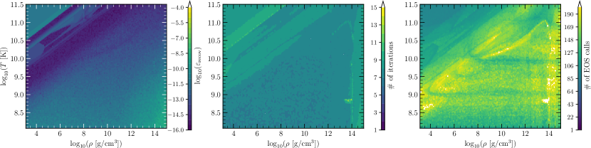
Figure 1: Average relative error $\varepsilon_{\rm recov}$ (left panel), number of iterations (middle panel), and EOS calls (right panel) required to reach the desired tolerance in recovering the primitive variables from the conserved ones. The example shown employs the LS220 EOS  Lattimer and Swesty (1991) with parameter values $W=2$ and $Y_{e}=0.1$. The magnetic field is nonzero and set so that the pressure ratio is $b^{2}/2p=10^{-3}$, with $b^{2}:=b_{i}b^{i}$ being the strength of the magnetic field in the fluid frame.

III.5 Performance of the primitive-recovery scheme

We here evaluate the performance of our primitive-recovery scheme presented in the previous section in terms of accuracy and efficiency, and compare it to other schemes used in GRMHD simulations and that are either refereed to as 1D Neilsen et al. (2014); Newman and Hamlin (2014); Palenzuela et al. (2015), 2D Noble et al. (2006); Antón et al. (2006), or 3D Cerdá-Durán et al. (2008), depending on the dimensionality of the master root-finding function. Furthermore, to ensure a fair comparison with previous primitive-recovery schemes that use tabulated EOS, we adopt two of the tests mentioned in Siegel et al. (2018) and follow the same criteria outlined there, which include considerations of speed, accuracy, and robustness (see Sec. 4.1 of Siegel et al. (2018) for additional information). In both tests considered here – and for consistency with other previously published results – we have used the LS220 tabulated EOS Lattimer and Swesty (1991).

In the first test, we use ranges of $\rho$ and $T$ that cover the valid regions of the EOS table. More specifically, we select primitive variables with the following values: a Lorentz factor of $W=2$, a ratio of magnetic-to-fluid pressure of $b^{2}/(2p)=10^{-3}$, and an electron fraction of $Y_{e}=0.1$. Figure 1 presents the average relative error as a function of the number of iterations and EOS calls required for convergence. More precisely, we compute the average relative error as Siegel et al. (2018)

$$\varepsilon_{\rm recov}:=\frac{1}{5}\sum^{5}_{i=1}\left|1-\frac{\bm{P}_{i,\mathrm{recov}}}{\bm{P}_{i,\mathrm{orig}}}\right|\,,$$ (40)

where $\bm{P}_{i,\mathrm{recov}}$ refers to the five recovered primitive variables $(\rho,v^{i},\epsilon,B^{i},Y_{e})$, while $\bm{P}_{i,\mathrm{orig}}$ indicates the original values of the primitives. Furthermore, we stop the iterations when a residual error of $\leq 5\times 10^{-9}$ is obtained for the maximum relative error in the iteration variables through our primitive-recovery scheme. Overall, Fig. 1 illustrates that across the entire parameter space encompassing $\rho$ and $T$, the average relative error $\varepsilon_{\rm recov}$, the average number of iterations, and the average number of EOS calls are found to be $7.84\times 10^{-12}$, $7.989$, and $135.8$, respectively.

With these results, and before entering in the details of the comparison, it is worth noting that multi-dimensional recovery schemes tend to require fewer EOS calls (about 3-8 times less) compared to 1D schemes (this was discussed also in Siegel et al. (2018)), but also a similar number of iterations (5-9), in order to reach converge. The high number of EOS calls in the effective 1D schemes is primarily due to the additional inversion steps caused by the use of the EOS table in terms of $T$ instead of $\epsilon$. Therefore, the number of EOS calls, and the associated computationally expensive interpolations, the table look-ups, and the root-finding procedures for the inversion of $\epsilon$ to $T$, can be taken as a direct proxy of the numerical costs.

A similar behaviour, i.e., few iterations, many EOS calls, is found also with our recovery scheme, which is effectively a 1D scheme with an additional inversion step from $\epsilon$ to $T$ using the table. However, when comparing our recovery scheme with the other schemes discussed in Ref. Siegel et al. (2018), we have found a clear improvement in terms of efficiency, as our approach requires significantly fewer EOS calls. At the same time, although our scheme requires a number of iterations that is similar to that reported in Refs. Palenzuela et al. (2015); Newman and Hamlin (2014), the mean number of EOS calls is $135.8$, which is to be compared respectively with $836$ for Ref. Palenzuela et al. (2015) and 331 for Ref. Newman and Hamlin (2014). In addition, our scheme exhibits a lower average relative error when compared to all other schemes, in particular within the regime relevant to realistic astrophysical problems, such as for rest-mass densities in the range $\rho\in[10^{8},10^{14}]\,\mathrm{g~{}cm^{-3}}$ and for the entire range of temperatures $T_{\rm min/max}$ of typical tabulated EOSs. More precisely, the schemes in Refs. Cerdá-Durán et al. (2008) and Newman and Hamlin (2014) yield the lowest average relative error among all the schemes, with values of $1.3\times 10^{-13}$ and $6.1\times 10^{-13}$, respectively. However, the accuracy in these schemes is not homogeneous and much higher in the upper left corner of the parameter space, while the relative error increases significantly for rest-mass densities typical of neutron stars. On the other hand, our scheme covers with high accuracy the entire parameter space with fewer than 12 iterations, except for a few points that require a larger number of iterations for convergence. Finally, no failures are found in contrast to what experienced with other schemes.

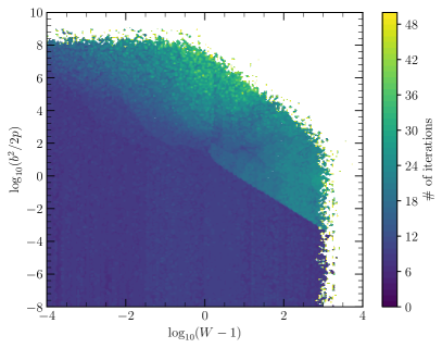
Figure 2: Number of iterations required to reach the desired tolerance in recovering the primitive variables from the conserved ones when using the LS220 EOS with parameters values $\rho=10^{11}\,\mathrm{g~{}cm^{-3}}$, $T=5\,\mathrm{MeV}=5.8\times 10^{10}\,\mathrm{K}$, and $Y_{e}=0.1$.

To further establish the robustness of our primitive-recovery scheme, we again follow Siegel et al. (2018) and conduct a second test that iterates over the parameter space of the Lorentz factor $W$ and the ratio of magnetic-to-fluid pressure $b^{2}/2p$, while maintaining fixed the values of $\rho=10^{11}\,\mathrm{g~{}cm^{-3}}$, $T=5\,\mathrm{MeV}$, and $Y_{e}=0.1$. Figure 2 illustrates the number of iterations required for convergence in this second test and shows that the maximum number of iterations in this parameter space is $51$; the white spaces indicate areas where the recovery process failed or the desired tolerance could not be achieved with the corresponding parameter sets. In full analogy with the performance of other schemes considered in Siegel et al. (2018), also our recovery scheme fails when the fluid becomes ultra-magnetized, i.e., when $b^{2}/2p\gtrsim 10^{8}$, or when the flow is ultra relativistic, i.e., $W\gtrsim 10^{3}$. However, our recovery scheme performs better than all other schemes, which either failed during recovery or required more than $25$ iterations to achieve a recovery when $W>10-100$.

In terms of robustness, our scheme exhibits a similar performance to that reported in Ref. Newman and Hamlin (2014), successfully recovering the primitive variables at $W=1000$, except when $b^{2}/2p>10^{-2}$. In such cases, the efficiency slightly degrades, and the number of iterations increases to $20-25$ for $W>10$. However, since it does not require initial guesses, or thermodynamic derivatives, or an initial bracket for the root $\mu_{+}$ in Eq. (21), and guarantees the existence and uniqueness of the root Kastaun et al. (2021), our recovery scheme can be employed reliably over a larger parameter space when compared to most other recovery schemes.

In summary, on the basis of the battery of sets performed, we conclude that the primitive-recovery scheme presented in Sec. III.4 provides higher robustness and accuracy when compared to other 1D and multi-dimensional schemes reported in Ref. Siegel et al. (2018) and requires the smallest number of EOS calls among all the effective 1D schemes. As a consequence of its robustness, no fail-safe strategy in the case of failed primitive recovery is needed in BHAC+.

III.6 Atmosphere treatment and error-handling policy

In analogy with other codes, the “atmosphere” – i.e., the spatial region of very low rest-mass density needed to avoid the failure of the solution of the GRMHD equations – is characterized by two basic parameters: the rest-mass density threshold, denoted as $\rho_{\mathrm{thr}}$, and the ratio between the density threshold and the atmosphere density $\xi:=\rho_{\mathrm{atm}}/\rho_{\mathrm{thr}}$. In all simulations conducted with BHAC+, these parameters are typically set to $\rho_{\mathrm{thr}}=10^{-14}$ and $\xi=0.9$, respectively. Furthermore, all cells with $\rho<\rho_{\mathrm{thr}}$ are identified as atmosphere and the corresponding values of the primitives variables are set as follows:

$$\rho=\rho_{\mathrm{atm}}\,, W=1\,, v^{i}=0\,,$$

$$\epsilon=\epsilon_{\mathrm{atm}}\,, Y_{e}=Y_{e,\mathrm{atm}}\,, p=p_{\mathrm{atm}}\,,$$

$$T=T_{\mathrm{atm}}\,, c_{s}^{2}=c^{2}_{s,\mathrm{atm}}\,, B=B_{\mathrm{atm}}\,.$$

where the value of the magnetic field in the atmosphere, $B_{\mathrm{atm}}$, is free to evolve as soon as the corresponding cell is pushed out of the atmosphere via a nonzero velocity.

When considering the atmosphere treatment in BHAC+, we need to distinguish the situation in which an analytical EOS is used from that in which the EOS is tabulated. In the former case, the polytropic EOS is applied to describe the properties of the atmosphere, so that the pressure is given by

$$p_{\mathrm{atm}}=K\rho_{\mathrm{atm}}^{\Gamma},$$ (41)

with $K=100$ and $\Gamma=2$ for the polytropic constant and polytropic index, respectively. On the other hand, the specific internal energy and the square of the sound speed in the atmosphere can be obtained analytically as (see, e.g.,  Rezzolla and Zanotti (2013))

$$\epsilon_{\mathrm{atm}} = \frac{K\rho_{\mathrm{atm}}^{\Gamma-1}}{\Gamma-1}\,,$$

$$c^{2}_{s,\mathrm{atm}} = \frac{p_{\mathrm{atm}}\Gamma(\Gamma-1)}{\rho_{\mathrm{atm}}(\Gamma-1)+p_{\mathrm{atm}}\Gamma}\,.$$

A different approach needs to be adopted when utilizing a tabulated EOS, in which case the neutrinoless $\beta$ equilibrium condition is employed. More specifically, at the beginning of the simulation, after setting $\rho_{\mathrm{atm}}$ and $T_{\mathrm{atm}}=T_{\mathrm{min}}$, a root-finding process is performed to determine the value of the electron fraction $Y^{\beta}_{e}$ that satisfies the neutrinoless $\beta$ equilibrium condition

$$0=\mu_{e}(Y_{e,i})+\mu_{p}(Y_{e,i})-\mu_{n}(Y_{e,i})\,,$$ (42)

where we employ Brent’s method within the interval $Y_{e,i}\in[Y_{e,\mathrm{min}},Y_{e,\mathrm{max}}]$ and with $\mu_{e/p/n}$ representing the chemical potentials accounting for the rest-mass of electrons, protons, and neutrons, respectively. Once $Y^{\beta}_{e}$ is determined, it is adopted as the electron fraction value for the atmosphere, $Y_{e,\mathrm{atm}}$. The remaining atmospheric quantities, namely $\epsilon_{\mathrm{atm}}$, $p_{\mathrm{atm}}$, and $c^{2}_{s,\mathrm{atm}}$, can be obtained through the EOS using $\rho_{\mathrm{atm}}$, $T_{\mathrm{atm}}$, and $Y_{e,\mathrm{atm}}$ for neutrinoless $\beta$-equilibrium matter.

III.7 Error-handling policy

It is not uncommon in modern relativistic GRMHD codes that physical conditions of low rest-mass density and high magnetization may lead to the generation of unphysical values of the matter quantities, especially in regions that are treated as atmosphere, or where round-off errors may develop, e.g., near the surface of compact objects or in ultra-relativistic flows. In order to ensure stable long-term simulations and maintain accurate evolutions, error-handling procedures play a crucial role in determining the criteria to be followed first to flag a problematic cell and second to correct its physical representation. In our strategy for treating problematic fluid cells, we incorporate some of the prescriptions described in Ref. Galeazzi et al. (2013) and adopt the following list of error-handling policies:

1. if $\rho>\rho_{\mathrm{max}}$, then mark as a fatal error.

2. if $\epsilon<\epsilon_{\mathrm{min}}$, then set $\epsilon=\epsilon_{\mathrm{min}}$.

3. if $\epsilon>\epsilon_{\mathrm{max}}$, then mark as a fatal error.

4. if $T<T_{\mathrm{min}}$, then set $T=T_{\mathrm{min}}$.

5. if $T>T_{\mathrm{max}}$, then mark as a fatal error.

6. if $Y_{e}<Y_{e,\mathrm{min}}$, then set $Y_{e}=Y_{e,\mathrm{min}}$.

7. if $Y_{e}>Y_{e,\mathrm{max}}$, then set $Y_{e}=Y_{e,\mathrm{max}}$.

8. if $\epsilon\leq\epsilon_{\mathrm{low}}(\rho,T_{\mathrm{min}},Y_{e})$, then within the inversion of $\epsilon$ to $T$ set $\epsilon=\epsilon_{\mathrm{low}}$ and $T=T_{\mathrm{min}}$.

9. if $\epsilon\geq\epsilon_{\mathrm{high}}(\rho,T_{\mathrm{max}},Y_{e})$, then within the inversion step of $\epsilon$ to $T$ set $\epsilon=\epsilon_{\mathrm{high}}$ and $T=T_{\mathrm{max}}$.

10. if $W>W_{\mathrm{max}}$, then, only in low rest-mass density region, we limit $W=W_{\mathrm{max}}$ and set $v=v_{\mathrm{max}}:=\sqrt{1-1/W^{2}_{\mathrm{max}}}$. The conserved density $D$ is kept fixed and we calculate $\rho=D/W_{\mathrm{max}}$.

Finally, while these policies are fully generic, they are systematically applied in the following five different scenarios:

1. after importing initial data;

2. before the inversion from $\epsilon$ to $T$;

3. after primitive recovery;

4. after reconstruction from the left and right-hand sides;

5. after restriction or prolongation steps following the mesh refinement.

IV Results

We next present a series of numerical tests aimed at assessing not only the accuracy and stability of BHAC+, but also its ability to import a timeslice from a fully numerical-relativity simulation provided by FIL and evolve it stably for timescales up to one second. These representative tests simulate various astrophysical systems with increasing degree of realism and complexity, hence, starting from oscillating nonrotating stars, to go over to rapidly rotating stars, magnetized and differentially rotating stars, the head-on collision of two neutron stars, and to conclude with the long-term BNS post-merger remnants. The tests span across different spatial dimensions, ranging from 1D to 2D and 3D, employing either spherical, cylindrical, or Cartesian coordinates, and different types of EOSs, from analytical to tabulated, as well as with varying spacetime conditions, including both fixed and dynamical spacetimes. Table 1 provides a summary of the parameters, dimensions, coordinate systems, and grid information for each set of initial data used in the various tests.

IV.1 Tests setup and initial conditions

In all simulations performed using FIL, the time integration of the full system of Einstein-Euler equations is performed using a Method of Lines (MOL) Rezzolla and Zanotti (2013), with a third-order Runge-Kutta method and a fixed CFL factor of $\mathcal{C}_{{}_{\rm CFL}}=0.2$. The GRMHD equations are solved with a two-wave Harten-Lax-van Leer-Einfeldt (HLLE) Riemann solver Harten et al. (1983); Einfeldt (1988), and a WENO-Z (Weighted Essentially Non-Oscillatory with Z characteristic) reconstruction (Borges et al., 2008) coupled to an HLLE Riemann solver Harten et al. (1983) (see Refs. Most et al. (2019a, 2021); Chabanov et al. (2023) for additional details). On the other hand, all the simulations performed with BHAC+ employ the Harten-Lax-van Leer (HLL) Riemann solver Harten et al. (1983), a Piecewise Parabolic Method (PPM) Colella and Woodward (1984), and a third-order Runge-Kutta (RK3) time integrator. A second-order Lagrange interpolation is used for the metric interpolation and the divergence-free constraint is enforced by using upwind constrained transport Olivares et al. (2019). Information on the coordinates used, the computational domain, the resolution on the coarsest level, and the number of refinement levels employed is presented in Table 1 for each simulation. For the adaptivity in the mesh-refinement process, we employ a Löhner error estimator Löhner (1987) based on the values of the rest-mass density.

Special and different care needs to be paid depending on the type of coordinates used for the simulations in BHAC+. In particular, in the case of cylindrical coordinates, the highest refinement level is set to be within a spherical region of radius $R<R_{\rm{in}}=30\,M_{\odot}\simeq 44.3\,\mathrm{km}$ and this is always sufficient to resolve the high-density region of the studied systems. In the case of spherical coordinates, however, a different strategy is necessary. This is because there is an inevitable accumulation of grid points near the center of the coordinate system represents a challenge because of the strict constraint on the timestep imposed by the CFL stability condition. For this reason, in the case of spherical coordinates we employ a single grid block covering an inner spherical region of radius $R_{\rm{core}}<1-2\,M_{\odot}\simeq 1.48-2.95\,\mathrm{km}$, which is not the first (highest) refinement level but the second one; this allows us to have good resolution near the coordinate center but not to be penalized by an excessively small timestep. The first refinement level is instead set within the spherical shell with $R_{\rm{core}}<R<R_{\rm{in}}=30\,M_{\odot}\simeq 44.3\,\mathrm{km}$, while the third (lowest) refinement levels covers the region with $R_{\rm{in}}<R<R_{\rm out}$, where $R_{\rm out}$ is the maximum value of the radial coordinate (see Tab. 1 where $R_{\rm out}=x^{r}_{\rm max}$), and thus contains the outer boundaries. This setup, while not fully exploiting the adaptive-mesh capabilities of BHAC+, results in a reasonable timestep constraint. Additionally, one of our tests (i.e., the 3D head-on in Table 1) requires a particular refinement structure in Cartesian coordinates. More specifically, we introduce five nested rectangular regions with the innermost having the highest refinement level, characterized by a volume of $90\times 40\times 40\,M_{\odot}^{3}\simeq 133\times 59\times 59\,\mathrm{km^{3}}$) and containing both stars at all times. Each side of outer refinement boxes having $(x,y,z)$ extents in solar masses given by $(10,10,10)$, $(20,30,30)$, $(110,30,30)$, and $(160,180,180)$.

Note that whenever importing initial data in BHAC+, we check the Löhner refinement criterion to establish whether to refine or coarsen the grid blocks and refill the initial data to the refined grids before the evolution in order to reduce the error induced by prolongation and restriction for the initial data. During the evolution, instead, we evaluate the Löhner refinement criterion every $10$ iterations to determine new refinement levels for all blocks.

Finally, for all simulations performed with BHAC+, the values of the CFL factor and of the efficiency parameter depend on the coordinate employed, so that $\mathcal{C}_{{}_{\rm CFL}}=0.3,0.3$, and $0.4$, while $\xi_{\rm eff}=1/10,1$, and $1/50$ for for cylindrical, Cartesian, and spherical coordinates, respectively. The only exceptions are represented by the tests involving the 3D head-on collision of two neutron stars and the 2D long-term evolution of the BNS remnant; in particular, for the head-on test we employ a Cartesian coordinate and a CFL factor $0.3$, while for the 2D long-term evolution the cylindrical coordinate and a CFL factor of $0.25$ are used. In both cases, different values of $\xi_{\rm eff}=1,1/3,1/10$ are employed to determine the optimal balance between computational costs and accuracy (see discussion in Secs. IV.6 and IV.7).

Test	Dim.	Coords.	Spacetime	EOS	$N_{\mathrm{ref}}$	$N_{1}\!\times\!N_{2}\!\times\!N_{3}$	$(N_{1}\!\times\!N_{2}\!\times\!N_{3})_{\mathrm{eff}}$	$\Delta x^{i}_{\mathrm{min}}$	$x^{i}_{\rm max}$	ID
								($10^{-2}$)
BU0-cow	1D	spher.	fixed	$\Gamma$-law	$1$	$640$	$640$	[$7.81$]	[$50$]	XNS
BU0-dyn	1D	spher.	dynamical	$\Gamma$-law	$1$	$640$	$640$	[$9.38$]	[$50$]	XNS
migration	2D	spher.	dynamical	$\Gamma$-law	$1$	$640\!\times\!32$	$640\!\times\!32$	[$9.38,5.33$]	[$60,\pi/2$]	RNS
magnetized-DRNS	2D	spher.	dynamical	$\Gamma$-law	$3$	$64\!\times\!64$	$256\!\times\!256$	[$39.10,0.61$]	[$100,\pi/2$]	XNS
DD2RNS-mr	2D	cylin.	dynamical	HSDD2	$5$	$32\!\times\!32$	$512\!\times\!512$	[$19.53,19.53$]	[$+100,+100$]	RNS
DD2RNS-hr	2D	cylin.	dynamical	HSDD2	$5$	$64\!\times\!64$	$1024\!\times\!1024$	[$9.77,9.77$]	[$+100,+100$]	RNS
head-on	3D	Cart.	dynamical	HSDD2	$5$	$128\!\times\!128\!\times\!64$	$2048\!\times\!2048\!\times\!1024$	[$19.53,19.53,19.53$]	[$\pm 200,\pm 200,+200$]	FUKA
DD2BNS-HO@20ms	2D	cylin.	dynamical	HSDD2	$10$	$16\!\times\!16$	$8192\!\times\!8192$	[$9.77,9.77$]	[$+800,+800$]	FIL
DD2BNS-HO@50ms	2D	cylin.	dynamical	HSDD2	$10$	$16\!\times\!16$	$8192\!\times\!8192$	[$9.77,9.77$]	[$+800,+800$]	FIL

Table 1: Summary of the simulations discussed in the paper and performed by BHAC+. The different columns report the name of the test, the number of spatial dimensions and the coordinates employed, the evolution of the spacetime, the EOS, the number of refinement levels ($N_{\rm ref}$), the number of cells on the coarsest level ($N_{1}\times N_{2}\times N_{3}$), the effective number of cells given the refinements ($(N_{1}\times N_{2}\times N_{3})_{\rm eff}$), the finest-cell sizes in the first, second, and third dimension $(\Delta x^{i}_{\rm min})$; depending on the coordinate system the units are either solar masses or radians), the maximum coordinate in the first, second, and third dimension $x^{i}_{\rm max}$ (domain), and the code providing the initial data. Information on the simulations run by FIL are reported in the main text.

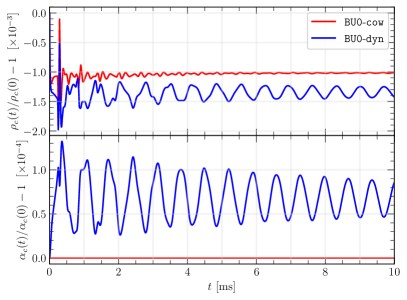
Figure 3: Top panel: Relative difference in the evolution of the central rest-mass density $\rho_{c}(t)$ when normalized to the initial one for two nonrotating stars when evolved in either the Cowling approximation (BU0-cow, red solid line) or with a dynamical spacetime within the CFC approximation (BU0-dyn, blue solid line). Bottom panel: the same as in the top one but for the central value of the lapse function $\alpha_{c}(t)$.

IV.2 TOV star with an ideal-fluid EOS

We start our validation of BHAC+ with a rather simple but complete test: the long-term oscillation properties of a nonrotating star. This test was first employed in a fully general-relativistic spacetime already in Ref. Font et al. (2002) and has been explored systematically in Ref. Dimmelmeier et al. (2006). Hence, we consider a nonrotating neutron-star model with a polytropic EOS having $\Gamma=2$ and $K=100$, a gravitational mass of $1.40\,{M_{\odot}}$, and a central rest-mass density of $\rho_{c}=1.28\times 10^{-3}=7.91\times 10^{15}\,{\rm g~{}cm}^{-3}$. This model was first introduced in Ref. Stergioulas et al. (2004) and is there referred to as “BU0”, and is also a reference model for the open-source code XNS Bucciantini and Del Zanna (2011); Pili et al. (2014). Given the symmetry of the problem and the flexible dimensionality of BHAC+, we carry out this first test in 1D spherical coordinates and an ideal-fluid ($\Gamma$-law) EOS, i.e., $p=\rho\epsilon(\Gamma-1)$, with $\Gamma=2$. The spacetime is either kept fixed in what is otherwise referred to as the “Cowling approximation”, (test BU0-cow) or evolved with the xCFC scheme (test BU0-dyn); in both cases the evolution is carried out for $10\,\mathrm{ms}$.

The upper panel of Fig. 3 shows the relative difference in the evolution of the central rest-mass density $\rho_{c}(t)$ with respect to the initial rest-mass central density, i.e., $\rho_{c}(0)$, for both the models BU0-cow and BU0-dyn. The lower panel of Fig. 3, on the other hand, shows the same but for the central value of the lapse function $\alpha_{c}(t)$. Since no explicit perturbation is introduced in both stars, the small oscillations are triggered by round-off errors and they remain harmonic and small in amplitude (i.e., $\lesssim 10^{-3}$) over the time of the solution.

The evolutions in Fig. 3 report a well-known behaviour (see, e.g., Font et al. (2002); Dimmelmeier et al. (2006); Radice et al. (2014)), namely, that the oscillations are more rapidly damped in the case of a fixed spacetime, simply because the dynamical coupling between the evolution of matter and the gravitational field is broken and a larger amount of mass is lost at the surface. Stated differently, in the Cowling approximation the gravitational fields cannot react to the local under- or overdensities caused by oscillations and matter is more easily lost from the stellar surface at each oscillation. When the spacetime is evolved, on the other hand, the amplitude of the oscillations is damped because of a small but nonzero numerical bulk viscosity Cerdá-Durán (2010); Chabanov and Rezzolla (2023).

What matters most in this test is that the frequencies of the numerical oscillations match the expected oscillation eigenfrequencies computed perturbatively, either in a fixed or in a dynamical spacetime. To this scope, Fig. 4 reports the power spectral density (PSD) of the Fourier transform of the function $\rho_{c}(t)$ over the $10\,\mathrm{ms}$ evolution of model BU0-dyn and compares it with the perturbative frequencies of the fundamental radial-oscillation mode ($F$-mode) and of its first overtone ($H_{1}$) Dimmelmeier et al. (2006). The relative differences between the two frequencies is $0.8\%$ for the $F$-mode and $0.7\%$ for the $H_{1}$-mode, with the numerical mode being systematically smaller, as expected from a nonlinear solution in a linear regime. Overall, the high accuracy of these results provide us with the first evidence of the correct implementation of the CFC approximation in BHAC+.

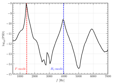
Figure 4: Power spectral density (PSD) of the evolution of the normalized central rest-mass density $\rho_{c}(t)/\rho_{c}(0)$ of the BU0-dyn test computed over a timescale of $10\,\mathrm{ms}$ as in the top panel of Fig. 3. Two clear peaks are visible in the PSD and show a very good match with the expected eigenfrequencies of the fundamental mode ($F$-mode, red dashed line) and of its first overtone ($H_{1}$-mode; blue dashed line) computed from perturbation studies Dimmelmeier et al. (2006).

IV.3 Migration test

Stepping up in complexity, we now consider a test that simulates a fully nonlinear scenario in which both the field and the matter variables undergo very rapid changes. The test in question, which is commonly referred to as the “migration test” was first introduced in Ref. Font et al. (2002) and has since been employed to test a variety of codes Cordero-Carrión et al. (2009); Bucciantini and Del Zanna (2011); Radice et al. (2014). In essence, this test studies the evolution of a nonrotating neutron star placed on the unstable branch of equilibrium configuration and which is triggered to “migrate” on the stable branch where it will find a stable configuration with the same rest mass after undergoing a series of large-amplitude oscillations. In this process, the star essentially expands very rapidly, converting its binding energy into kinetic energy, and then, via shock-heating, into internal energy.

Since this is purely a numerical test, we choose the neutron star to have a central rest-mass density of $\rho_{c}=7.993\times 10^{-3}\simeq 4.937\times 10^{15}\,{\rm g~{}cm}^{-3}$, and employ a polytropic EOS with $\Gamma=2$ and $K=100$, thus leading to an initial radius $R=4.06\,M_{\odot}=6.29\,\mathrm{km}$. The evolution, on the other hand, is carried out with an ideal-fluid EOS with the same adiabatic index. The stellar model is then evolved in 2D employing spherical polar coordinates within a dynamical spacetime and its dynamics compared with that obtained with FIL.

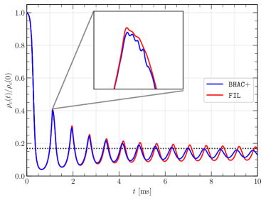
Figure 5: Evolution of the central rest-mass density normalized to the initial value in the migration test. Reported with solid lines of different color are the evolution by BHAC+ (blue line) and by FIL (red line). Note the excellent agreement especially over the first few oscillations; the black dotted line represents the central rest-mass density of the star on the stable branch having the same gravitational mass, which is higher than the asymptotic solutions since it does not account for the matter lost in the nonlinear shocks at the stellar surface.

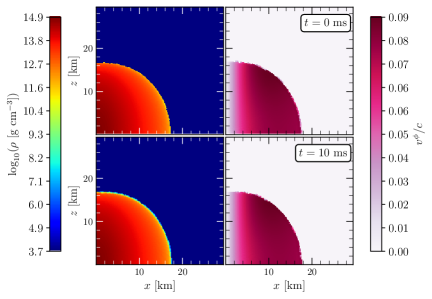
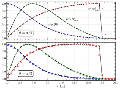
Figure 6: Left panel: 2D distributions of the rest-mass density (left column) and of the rotational velocity (right column) of a magnetized and differentially rotating star (test magnetized-DRNS in Table 1). The top row refers to the initial time $t=0$, while the bottom row to the final time $t=10\,\mathrm{ms}$, corresponding to about eight rotational periods, and showing a very good preservation of the axisymmetric equilibrium. Right panel: indicated with different symbols are the 1D profiles of the rest-mass density, of the angular velocity, and of the toroidal magnetic field, all normalized to their maximum values for the same test in the left panel. The top row displays the profiles at a polar angle $\theta=\pi/4$, while the bottom row shows them on the equatorial plane $\theta=\pi/2$. For all quantities, the dashed lines represent the initial profiles, which are well preserved even after eight rotational periods.

Figure 5 illustrates the evolution of the central rest-mass density normalized by its initial value at $t=0$, while the black dotted line represents the central rest-mass density of the neutron star on the stable branch with $\rho_{c}=1.346\times 10^{-3}$ having the same gravitational mass as the initial model (this value is higher than the asymptotic solutions since it does not account for the matter lost in the nonlinear shocks at the stellar surface). Overall, our results are qualitatively consistent with previous studies, either in full general relativity Font et al. (2002); Radice et al. (2014), or employing the CFC approximation Cordero-Carrión et al. (2009); Bucciantini and Del Zanna (2011), and exhibit the well-know behaviour in terms of peak amplitudes, density at the first and second maxima, the non-harmonic nature of the density oscillations, etc. However, for a more quantitative comparison, we present in Fig. 5 also a direct comparison of the corresponding evolution carried out by FIL in full general relativity and with very similar spatial resolution. Notwithstanding the intrinsic approximations associated with the CFC approach, the similarities between the two curves, especially in the most nonlinear part of the evolution (i.e., $t\lesssim 2\,{\rm ms}$) is quite remarkable; the similarities between the two evolutions persist up to $t\lesssim 5\,{\rm ms}$, after which the more dissipative features of the CFC approximation appear and phase differences emerge in the evolution. We should recall, in fact, that, in addition to the less accurate spacetime evolution, BHAC+ utilizes a second-order accurate finite-volume scheme for the solution of the GRMHD equations, while FIL employs a fourth-order accurate – and hence less diffusive – finite-difference method. Overall, however, also this migration test provides an important validation of the correct implementation of the CFC solver in a 2D scenario.

IV.4 Magnetized and differentially rotating star

All of the tests presented so far referred to configurations with a zero magnetic field. In order to validate the ability of BHAC+ to properly solve the GRMHD equations in a dynamical spacetime, we consider the evolution of a magnetized and differentially rotating star Bucciantini and Del Zanna (2011); Cheong et al. (2021). To this scope, we again use XNS Bucciantini and Del Zanna (2011) to generate a self-consistent magnetized star with a purely toroidal magnetic field and in differential rotation. In particular, the initial stellar model was modeled as following the $j$-constant rotation law Komatsu et al. (1989) with central angular velocity $\Omega_{c}=2.575\times 10^{-2}$ and differential-rotation parameter $A^{2}=70$, and a polytropic EOS with $\Gamma=2$ and $K=100$ (this test is referred to as magnetized-DRNS in Table 1). The resulting initial central rest-mass density is $\rho_{c}(0)=1.28\times 10^{-3}=7.91\times 10^{15}\,{\rm gm~{}cm}^{-3}$ and we prescribe the magnetic-field strength $B:=\sqrt{B_{i}B^{i}}$ with the law Kiuchi and Yoshida (2008)

$$B:=\left\{\begin{array}[]{lr}{K_{m}(\alpha^{2}\varpi^{2}\rho h)^{m}}/({\alpha\varpi})\,,&\text{for}~{}\rho>10^{-9}\\ 0\,,&\text{for}~{}\rho\leq 10^{-9}\end{array}\right.$$ (43)

where $\varpi:=\psi^{2}r\sin\theta$ is the generalized cylindrical radius, with $r$ and $\theta$ being the spherical radial and polar coordinates; in practice, we set $m=1$ and $K_{m}=3$. As remarked in Refs. Bucciantini and Del Zanna (2011); Cheong et al. (2021), the magnetic field in this star reaches a maximum value of $\sim 5\times 10^{17}\,\mathrm{G}$, thus accounting for $\sim 10\%$ of the total internal energy of the star and providing a non-negligible change in the underlying equilibrium.

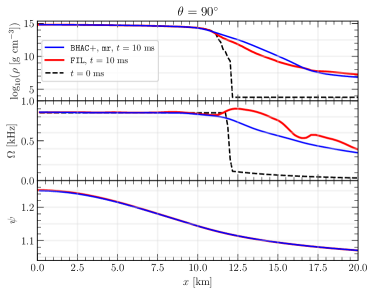
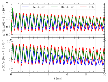
Figure 7: Left panel: 1D profiles at $\theta=90^{\circ}$ and at $t=10\,\mathrm{ms}$ of the rest-mass density (top row), of the angular velocity (middle row), and of the conformal factor (bottom row) for a rapidly and uniformly rotating neutron star (test DD2RNS-mr in Table 1). Solid lines of different color refer to the evolutions carried out by BHAC+ (blue line) or FIL (red line) showing a very good preservation of the equilibrium in the high-density regions of the star. The deviations from the initial profiles at $t=0\,\mathrm{ms}$ (black dashed lines) are comparable in the two codes and are typical of simulations of rapidly rotating stars (note the logarithmic scale employed here). Right panel: Evolution of the relative difference in the central rest-mass density (top row) and of the conformal factor (bottom row) for the same model reported in the left panel and the same convention for the line types. In addition, each row contains also the data of a high-resolution simulation (DD2RNS-hr, green solid line), highlighting how the differences with FIL can be decreased by a higher spatial resolution.

Once the initial stellar model is imported in BHAC+, we evolved the system in 2D using spherical coordinates and the same ideal-fluid EOS employed in the previous test for a duration of $10\,\mathrm{ms}$. The left panel of Fig. 6 shows the 2D slices of the rest-mass density and of the rotational velocity, $v^{\phi}$, at two different times, $t=0$ (upper part) and $t=10\,\mathrm{ms}$ (lower part). Clearly, a direct and qualitative comparison of the two 2D slices shows the ability of the code to retain an accurate description of the stellar model over more than eight spinning periods. The right panel of Fig. 6 shows instead a more quantitative comparison of the radial profiles of the rest-mass density, the linear rotational velocity $v^{\phi}$, and toroidal magnetic field $B^{\phi}$ at $t=0$ and $t=10\,\mathrm{ms}$ which are normalized by their maximum values. Furthermore, the upper part of the panel refers to the diagonal direction ($\theta=\pi/4$), while the lower panel to the equatorial one ($\theta=\pi/2$). We note that there on both angles there are minor distortions in the rotational velocity $v^{\phi}$ around $r\approx 17$ $\mathrm{km}$, where the low-density atmosphere interfaces with the high-density neutron star. The sharp gradient introduced by the stellar surface oscillates as a result of the round-off perturbations exhibiting a behavior consistent with the findings of Ref. Bucciantini and Del Zanna (2011). Overall, the results of this test further demonstrate that BHAC+ is capable of stably simulating a rapidly configuration stellar configuration with a strong magnetic field and over several rotation periods.

IV.5 Rapidly and uniformly rotating star with tabulated EOS

Next, we validate our new code by evolving a rapidly and uniformly rotating neutron star with a rotation rate close to the mass-shedding limit and described by a tabulated, finite-temperature EOS, specifically the HSDD2 EOS Hempel and Schaffner-Bielich (2010). Our initial data is computed as an axisymmetric equilibrium model using the RNS code Stergioulas and Friedman (1995) with angular velocity $\Omega=2.633\times 10^{-2}=850.85\,2\pi\,{\rm Hz}$ and is assumed to be in a neutrinoless $\beta$-equilibrium state with $T=T_{\mathrm{min}}$. The evolution in BHAC+ is performed in 2D with cylindrical coordinates and $z$-symmetry while, at the same time, we carry out an analogous evolution with FIL in Cartesian coordinates with the same resolution over the star (this is the test DD2RNS-mr in Table 1). To quantify the resolution dependence of BHAC+, we perform an additional simulation with BHAC+ having a resolution that is twice that used in FIL (this is the test DD2RNS-hr in Table 1).

The left panel of Fig. 7 illustrates the profiles on the equatorial plane (i.e., $z=0$) of the rest-mass density $\rho$ (top panel), of the angular velocity $\Omega$ (middle panel), and of conformal factor $\psi$ (bottom panel) at the initial time (black dotted line) and at $t=10\,\mathrm{ms}$, both for BHAC+ (blue solid line, case DD2RNS-mr) and FIL (red solid line). Remarkably, after eight rotation periods, all the matter quantities in the stellar interiors (i.e., $x\lesssim 12\,\mathrm{km}$) are well preserved, with only small deviations from the initial data despite the very extreme properties of the stellar model. This is true both for the data obtained with BHAC+ and with FIL; an even better agreement is found in the conformal factor, where the relative differences are less than $\simeq 0.15\%$.

The right panel of Fig. 7, on the other hand, reports the relative differences in the evolution of the central rest-mass density $\rho_{c}$ and of the conformal factor $\psi_{c}$ when compared to their initial values. Note also that in the case of the simulations carried out by BHAC+, we report evolutions with two different resolutions. This shows that as the resolution of BHAC+ is increased, the differences to the evolution in FIL decreases and the small de-phasing observed in the case of the medium-resolution simulation decreases significantly. The oscillations in $\rho_{c}$ and $\psi_{c}$ show relative variations in the high-resolution simulations that are less than $10^{-2}$ and $10^{-4}$, respectively.

Overall, bearing in mind that FIL uses high-order methods and the full evolution of the spacetime, the agreement with BHAC+, already at comparatively small resolutions and in simulating a rather challenging stellar model, confirms the ability of BHAC+ and of the CFC approximation to accurately reproduce in 2D results from a full 3D numerical-relativity code. In the following section we will demonstrate that this is also the case in full 3D simulations.

IV.6 Head-on collision of two neutron stars

We next discuss the head-on collision of two neutron stars as a 3D test to validate the full implementation of the set of equations and explore conditions of spacetime time curvature and matter dynamics that are very similar to those encountered in a binary merger from quasi-circular orbits Musolino and Rezzolla (2023), but that can be tested at a fraction of the computational cost (this test is indicated as head-on in Table 1). Indeed, the head-on collision of two stars has a long history and has been in the past employed to actually study the dynamics of critical phenomena Kellerman et al. (2010) or the formation of black holes for ultrarelativistic initial speeds East and Pretorius (2013); Rezzolla and Takami (2013). Furthermore, because of the minimal influence of gravitational waves, this scenario is also particularly suited for assessing codes utilizing the CFC approximation and allows us to compare once again the solutions obtained with FIL and BHAC+.

The initial data of FIL is generated using the FUKA code Grandclement (2010); Papenfort et al. (2021); Tootle (2023), which computes the initial data timeslice by solving the eXtended Conformal Thin Sandwhich (XCTS) system of equations Pfeiffer and York (2005); Papenfort et al. (2021). The initial data is obtained by first computing the isolated 3D solutions of the stars prior to constructing a spacetime representing the binary system. However, unlike the implementation discussed in Refs. Papenfort et al. (2021); Tootle (2023), we approximate the solution by superimposing two isolated solutions and re-solving the XCTS constraint equations where, however, some care must be taken as we will discuss shortly.

The initial guess of the head-on is generated by superimposing the isolated stellar solutions such that, for a given spacetime or source field $X$, the initial guess in the binary is constructed as Tootle (2023); Tootle and Rezzolla (2024)

$$X_{\rm bin}\left(\bm{x}\right) :=\Xi+\kappa_{1}\left(X_{1}\left(\bm{\hat{x}_{1}}\right)\!-\!\Xi\right)+\kappa_{2}\left(X_{2}\left(\bm{\hat{x}_{2}}\right)\!-\!\Xi\right)\,,$$ (44)

$$\kappa_{1,2} :=\exp\left[-\left(\frac{r_{1,2}}{d_{0}/2}\right)^{4}\right]\,,$$ (45)

$$\bm{\hat{x}}_{1,2} :=\bm{x}-\bm{{x}}_{c1,c2}\,,$$ (46)

where $\Xi$ is the asymptotic value for a given field (e.g., $\psi=\alpha=1$, $\beta^{i}=0$, etc), $d_{0}$ is the initial separation, $\bm{{x}}_{c1,c2}$ are the location of the neutron-star centers, and $\kappa_{1,2}$ represent the “decay parameters” centered about the respective neutron-star solution, such that the solution is exactly the isolated solution near the neutron star and then decays to flat spacetime further away. The decay behaviour of the solutions is controlled by the $4^{\rm th}$ power in the exponential, while the decay distance is controlled by the weight factor $d_{0}$. This approach is analogous to that employed in Ref. Helfer et al. (2022) for the head-on collision of boson stars and was inspired by previous works Lovelace et al. (2008); Foucart et al. (2008), though the application was focused on fixing background metric quantities instead of generating an initial guess for obtaining an initial-data solution.

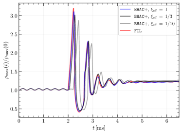
Figure 8: Evolution of the maximum rest-mass density normalized to the initial value in the 3D head-on collision test. The red line represents the result of FIL , while the blue line shows the evolution in BHAC+. Also shown with a black and gray solid line are the evolutions with different efficiency ratios, namely $\xi_{\rm eff}=1/3$ and $1/10$, respectively. The blue solid line is obtained with $\xi_{\rm eff}=1$ and is obviously the closest to the FIL evolution.

Since the initial time slice is not (quasi-)stationary and we no longer have a notion of conservation along fluid-lines, we are not able to strictly enforce hydrostatic equilibrium by solving the Euler equation. Instead, we adopt an approach similar to that used in Ref. Papenfort et al. (2021), where we relax this constraint and simply rescale the fluid quantities by a constant fixed by enforcing a fixed rest-mass. Thus, the fluid description of each neutron star will systematically scale as a function of the Lorentz factor $W$ due to the presence of the companion object. For this reason, we set the initial separation between the two stars to $d_{0}=60\,M_{\odot}\simeq 89.4\,{\rm km}$, such that the solutions are minimally rescaled while still resulting in a computationally efficient setup. It is important to note that relaxing the hydrostatic equilibrium is also a necessary step to obtain eccentricity reduced initial data, the effects of which have been discussed previously Tichy et al. (2019); Papenfort et al. (2021).

To further test the interfacing of FIL with BHAC+, the initial data from FUKA is first imported from FIL and then “handed-off” to BHAC+ so that the two codes have initial data that is equivalent to the one they exchange in a typical HO situation. The initial velocity of two neutron stars is set to zero, and their mass is set so as to avoid black-hole formation, i.e., they have an ADM mass $M_{{}_{\rm ADM}}=0.91\,M_{\odot}$ Musolino and Rezzolla (2023), and are described by the HSDD2 EOS Hempel and Schaffner-Bielich (2010). The finest refinement level of the two codes contain both of the neutron stars, have a grid resolution of $\simeq 0.2\,M_{\odot}\simeq 298\,\mathrm{m}$; for simplicity and a closer comparison, both the resolution and the grid structure is not varied during the evolution.

Figure 8 reports the evolution of the maximum rest-mass density normalized to its initial value as obtained by BHAC+ (blue solid line) and by FIL (red solid line). Note the very good agreement despite the very different set of field equations solved. In particular, it is remarkable that not only the time of the collision (i.e., when the central rest-mass density deviates most significantly from its initial value) differ by $\lesssim 1.3\%$, but also that the maximum and minimum changes in the maximum rest-mass density are very similar and differ by $\lesssim 4.9\%$ at most, while the differences in the asymptotic equilibrium values of the collision remain below $\simeq 0.4\%$. Note also that the variations in the fluid variables in this case are much more severe and extreme than what simulated in the case of the migration test (compare Fig. 8 with Fig. 5).

Also shown in Fig. 8 are examples of evolutions with different efficiency ratios and hence different computational efficiency. More specifically, while the blue solid line refers to $\xi_{\rm eff}=1$, the black and gray solid lines refer to $\xi_{\rm eff}=1/3$ and $1/10$, respectively. Note that, as expected, the comparison with the FIL evolution are worse in these cases, but also that the differences remain $\lesssim 10\%$ in the maximum variation of the central density, while the actual fundamental frequency of oscillation or the final central rest-mass density of the collision remnant differ by $\lesssim 3\%$. These differences – which are measured in the most extreme conditions of spacetime curvature expected in BNS mergers and are therefore to be taken really as upper limits – need to be contrasted with the corresponding gain in computational costs. More specifically, given similar resolution between two codes, considering that BHAC+ is about $3.5~{}(4.6)~{}[6.3]$ times faster than FIL for comparable resolutions when setting $\xi_{\rm eff}=1~{}(1/3)~{}[1/10]$, it becomes clear that a systematic error of a few percent can be tolerated over timescales of seconds when it comes with a gain of about a factor four to six in computational costs. Furthermore, additional gains can come from a better coordinate system and mesh refinement structure, by the use of even smaller values of $\xi_{\rm eff}$ at later times as the spacetime dynamics is much less severe, and, more importantly, by the considerable difference in the CFL constraint when considering the sound speed in place of the speed of light. Note that it is not difficult to show analytically that the computational gain $\bar{\gamma}$, i.e., the ratio of operations in a fully general-relativistic code (e.g., FIL ) and of constraint-solving code (e.g., BHAC+ ), is $\bar{\gamma}=(1+\xi_{\rm eff}c_{s}/c)/[(1+\xi_{\rm eff})c_{s}/c]$. Hence, $\bar{\gamma}\to c/c_{s}$ in the limit of $\xi_{\rm eff}\to 0$. Furthermore, because $\xi_{\rm eff}$ can be decreased with increasing spatial resolution, the computational gain actually increases when performing simulations with higher resolutions.

Figure 9 offers a comprehensive comparison of the 2D rest-mass density and temperature distributions of BHAC+ (depicted in the left part of each principal plane) and FIL (depicted in the right part of each principal plane). The different panels refer to different and representative times during the collision and the top-left panel in Fig. 9, in particular, reports the instant when the two neutron stars start colliding at $t\simeq 1.89\,{\rm ms}$. The comparison reveals a high degree of similarity between the two codes, although small differences do emerge. In particular, and as expected, the atmosphere surrounding FIL is hotter and denser than that of BHAC+. This discrepancy is mostly attributed to the different order at which the GRMHD equations are solved in the two codes with high-order schemes being normally more sensitive to small shocks at the stellar surface and hence to very small mass losses [see, e.g., Refs. Radice and Rezzolla (2012); Radice et al. (2014); Guercilena et al. (2017) for a discussion]. Note also that in this pre-merger phase both codes suffer from small failures in the temperature near the stellar surface and once again these are produced by the small rest-mass density fluctuations near the surface, which, in turn, are amplified by the high-power dependence of the temperature on these oscillations; when comparing the behaviour of the internal specific energy, in fact, these oscillations are essentially absent. The top-right panel of Fig. 9 shows instead the same quantities at the instant of maximum compression at $t\simeq 2.26\,{\rm ms}$ (see also the first peak in Fig. 8). At this time, matter experiences extreme compression in the $x$-axis direction (the collision is along the $x$-axis), leading to a peak temperature of approximately $50\,{\rm MeV}$ in the central region as a result of the collision of the two strong shocks fronts. The rest-mass density and temperature profiles in both codes exhibit striking similarity and some differences appear only in the very low-density regions of the FIL evolution, which is absent in the BHAC+ results. The bottom-left panel refers instead to the instant of minimum compression at $t\simeq 2.47\,{\rm ms}$ (see also the first minimum in Fig. 8), and shows that as a result of the bounce and change of sign in the bulk linear momentum, matter is expelled back in the $x$-axis direction producing a strong reverse shock at the surface of the merged object, so that the remnant has a low-density, low-temperature core produced by the induced rarefaction wave. Finally, the bottom-right panel shows to the stable remnant at $t\simeq 6.47\,{\rm ms}$, which exhibits a high-temperature mantle relative to the shocked material and a comparatively cooler core.

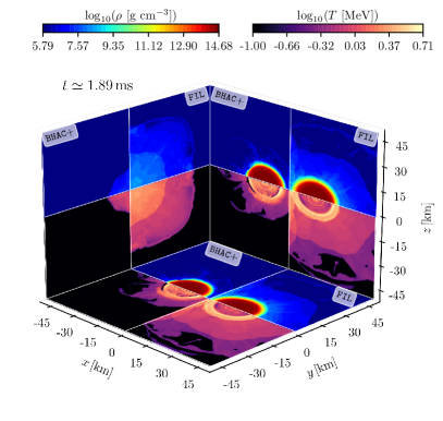
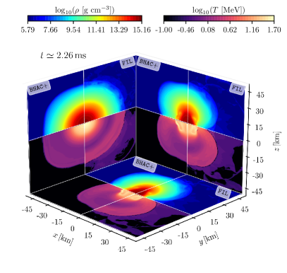
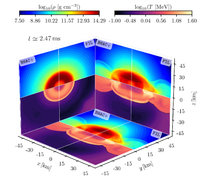
Figure 9: 2D comparison on the principal planes of the rest-mass density and temperature between in the head-on collision of two neutron stars (test head-on) as computed by BHAC+ (left part of each plane) and FIL (right part of each plane). In each column, the top part of each panel reports the rest-mass density, while the bottom part shows the temperature. Finally, the four panels refer to four different times, namely, the instant when the two neutron stars start colliding (top-left panel, $t\simeq 1.89\,{\rm ms}$), that of the maximum compression (top-right panel, $t\simeq 2.26\,{\rm ms}$), that of the minimum compression (bottom-left panel, $t\simeq 2.47\,{\rm ms}$), and that of the late-time evolution (bottom-right panel, $t\simeq 6.47\,{\rm ms}$). Note that the colorbars are different in the four panels and the use of negative-$z$ regions is done for visualization purposes only since the simulations actually employ a symmetry across the $z=0$ plane. Finally, note the very good agreement between the two evolutions despite the difference in coordinate systems, truncation order in the solution of the GRMHD equations, and different treatment of the spacetime evolution.

In summary, the remarkably good agreement between the two fully 3D evolutions despite the difference in coordinate systems, truncation order in the solution of the GRMHD equations, and different treatment of the spacetime evolution provides very convincing evidence for the ability of the CFC approximation to effectively model gravitational effects, particularly when the non-diagonal terms of the spatial metric tensor in the system are anticipated to be negligible, as it is the case during the free-fall stage preceding the collision.

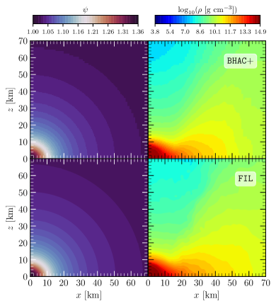
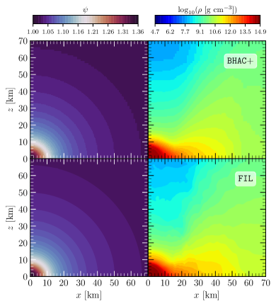
Figure 10: Left panel: 2D slices of the conformal factor (left) and of the rest-mass density (right) for a BNS post-merger remnant at $\bar{t}=50\,\mathrm{ms}$ as evolved by BHAC+ (top part of the panel) and by FIL (bottom part); the data has been handed-off at $t_{\mathrm{HO},1}=20\,\mathrm{ms}$. Right panel: The same as on the left but at $\bar{t}=100\,\mathrm{ms}$ and evolved with data handed-off at $t_{\mathrm{HO},2}=50\,\mathrm{ms}$ (see Fig. 11 for a quantitative comparison in 1D).

IV.7 Long-term evolution of a post-merger remnant

The next and final test we present is related to the 2D long-term (i.e., for about one second) evolution of the remnant of a BNS merger. A number of recent studies (see, e.g.,  Kastaun and Galeazzi (2015); Hanauske et al. (2017); Fujibayashi et al. (2017)) have shown that the BNS post-merger remnant relaxes into a nearly axisymmetric and quasi-stationary state after a few tens of milliseconds after the merger event. Furthermore, after approximately $50\,\mathrm{ms}$ after the merger, the absolute magnitude of the non-diagonal components of $\tilde{\gamma}_{ij}$ from FIL become very small, with relative differences with respect to the corresponding flat components that is $\lesssim 2\%$. Under these conditions, a more efficient and less expensive treatment of the spacetime evolution is particularly useful, especially for long-term evolutions at high resolutions. Of course, in order for BHAC+ to perform such an evolution it requires a consistent initial data and this can only be provided by a full-numerical relativity code, such a FIL, and the HO procedure described in Sec. III.3.

In practice, after constructing the initial data for a binary system of neutron stars with equal masses of $M=1.40~{}\,{M_{\odot}}$ in irrotational quasi-circular equilibrium and zero magnetic field with FUKA, we evolve the system with FIL well past the merger. The evolution is handled using five levels of mesh refinement and with the highest-resolution level having a spacing of $0.2\,M_{\odot}\simeq 0.295\,{\rm km}$. Defining $t$ and $t_{\mathrm{mer}}$ respectively as the times since the start of the simulation and the merger time, we define the retarded time as $\bar{t}_{\mathrm{HO}}:=t-t_{\mathrm{mer}}$ and fix the HO time from FIL to BHAC+ to a specific value of $\bar{t}$. Since the time of HO represents an important (and to some extent arbitrary) aspect of the long-term evolution, and in the spirit of assessing its impact, we have carried out two distinct simulations with HO at $t_{\mathrm{HO},1}:=20\,\mathrm{ms}$ and $t_{\mathrm{HO},2}:=50\,\mathrm{ms}$, respectively.

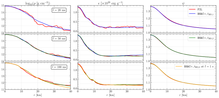
Figure 11: 1D slices at $z=0$ of the rest-mass density (left column), of the specific internal energy (middle column) and of the conformal factor (right column) for a BNS post-merger remnant at different times, i.e., $\bar{t}=20\,\mathrm{ms}$ (top row, test DD2BNS-HO@20ms), $\bar{t}=50\,\mathrm{ms}$ (middle row, test DD2BNS-HO@50ms) and $\bar{t}=100\,\mathrm{ms}$ (bottom row, test DD2BNS-HO@50ms). While the FIL data is always indicated with a red line, the BHAC+ data is shown with different colors depending on the HO time, i.e., with a blue solid line in the top row for $t_{\mathrm{HO},1}$ and with a green solid line in the middle and bottom rows for $t_{\mathrm{HO},2}$. Also reported with an orange solid line in the bottom row is the BHAC+ evolution at $t=1000\,{\rm ms}$ (see Fig. 10 for a more qualitative comparison in 2D).

We start our comparison by showing in Fig. 10 the 2D slices of the conformal factor $\psi$ (left part of each panel) and of the rest-mass density $\rho$ (right part of each panel) at two representative times, i.e., $\bar{t}=50\,\mathrm{ms}$ (left panel) and $\bar{t}=100\,\mathrm{ms}$ (right panel) respectively. Furthermore, for each panel, the top parts report the solutions from BHAC+ when the HO is made at $t_{\mathrm{HO},1}$ (left panel) or $t_{\mathrm{HO},2}$ (right panel), while the bottom part shows the solution relative to the FIL evolution restricted to the slice at $y=0$. Overall, the eight sub-panels shown in Fig. 10 indicate that, at least qualitatively, the solutions coming from the two codes are remarkably similar despite the differences in the approaches for the evolution of the spacetime and the different dimensionality (3D for FIL and 2D for BHAC+). Of course, there are two main reasons for this very good match. First, the gravitational fields characterising the remnant are comparatively weak and rather slow-varying, so that the CFC approximation provides a very good description. Second, by the time the HO is made at $t_{\mathrm{HO},1}$, the remnant is significantly axisymmetric, so that the azimuthally averaged description of the remnant made by BHAC+ matches very well the fully-3D solution computed with FIL.

Figure 11 goes from the qualitative description of Fig. 10 to a more quantitative one by reporting the 1D slices at $z=0$ for the solution obtained by BHAC+ and by FIL  (in this case the data is extracted at $y=z=0$; red solid lines) and at three representative times, namely, $\bar{t}=20\,\mathrm{ms}$ (top row), $\bar{t}=50\,\mathrm{ms}$ (middle row), and $\bar{t}=100\,\mathrm{ms}$ (bottom row) and for three different quantities, the rest-mass density (left column), the specific internal energy (middle column), and the conformal factor (right column). Note that in the case of the BHAC+ evolutions, we distinguish the data coming from $t_{\mathrm{HO},1}$ (blue solid lines in the top and middle rows) from that obtained when the HO is instead done at $t_{\mathrm{HO},2}$ (green solid lines in the middle and bottom rows). Note also that simulation by FIL is carried out till $\bar{t}=100\,{\rm ms}$, while the BHAC+ simulation with $t_{\mathrm{HO},1}$ till $\bar{t}=50\,{\rm ms}$, and that with $t_{\mathrm{HO},2}$ is performed till $\bar{t}=1.0\,{\rm s}$. Finally, shown instead with an orange solid line in the bottom row is the solution from BHAC+ at the final time of $1000\,{\rm ms}$.

Let us first compare the behaviour of the rest-mass density (left column) in the three different snapshots. Overall, it is clear that BHAC+ can reproduce the structure of the binary merger remnant very well, especially in the inner regions (i.e., $r\lesssim 10\,{\rm km}$) and quite independently of the HO time. Obviously, since the BHAC+ simulations are in 2D only, the corresponding profiles are smoother than those from FIL but the differences are apparent only when reported in a logarithmic scale, as we do in Fig. 11. Note also that the rest-mass profile in the remnant does not change considerably between $\bar{t}=100\,{\rm ms}$ (which represents the last time of the solution from FIL) and $\bar{t}=1000\,{\rm ms}$, with the structure of the remnant from BHAC+ being only slightly more diffused than that from FIL (cf., different profiles from $10\lesssim r\lesssim 20\,{\rm km}$).

Similar considerations apply also to the specific internal energy (middle row), where the BHAC+ solution with $t_{\mathrm{HO},2}$ (red solid line) shows a better agreement with the reference FIL solution as compared to that with $t_{\mathrm{HO},1}$ (blue solid line). The evolution of the temperature profile, on the other hand, can show more visible differences and is more sensitive on the HO time (not shown in Fig. 11). More specifically, the BHAC+ solution with $t_{\mathrm{HO},1}$ shows larger values of the temperature in the region $5\lesssim r\lesssim 20\,{\rm km}$, and smaller values in the more internal regions of the remnant, i.e., for $r\lesssim 5\,{\rm km}$; furthermore the temperature profile in BHAC+ in this inner core also exhibits oscillations that have small amplitude and short wavelengths. The origin of these differences can be attributed to three main origins. First, the initialization of the CFC field variables on the initial slice inevitably introduces fluctuations that are magnified in the behaviour of the temperature. Second, the initial differences in $\epsilon$ and $Y_{e}$ between FIL and BHAC+ are of the same order as those in $\rho$ and, especially after metric initialization, such initial differences become larger when the new constraints are satisfied. As a result, the accuracy of the calculation of the temperature as a function $T=T(\rho,\epsilon,Y_{e})$ – which already suffers from a poor resolution of the tabulated EOS at these regimes and from a high-power dependence of $T$ from $\epsilon$ in regions of high rest-mass density – is further affected. Third, the small fluctuations in the temperature produced in the conversion from $\epsilon$ to $T$ in the table are more easily averaged in a 3D simulation (where every cell has six neighbours to average with) than in a 2D simulation. Indeed, we observe that these oscillations are absent in the 3D head-on simulation presented in Sec. IV.6.

Finally, the right column of Fig. 11 reports the profiles of the conformal factor following the same convention in terms reported times and of HO times as in the left and middle columns. The comparison in this case is even simpler to describe and it is clear that the differences are very small for all the configurations considered. More specifically, the the largest absolute relative differences in the rest-mass density [conformal factor] at $\bar{t}=20\,\mathrm{ms}$ (FIL vs BHAC+ with $t_{\mathrm{HO},1}$), $\bar{t}=50\,\mathrm{ms}$ (FIL vs BHAC+ with $t_{\mathrm{HO},1}$), and $\bar{t}=100\,\mathrm{ms}$ (FIL vs BHAC+ with $t_{\mathrm{HO},2}$) are respectively $1.18\%$ [$0.05\%$], $0.17\%$ [$0.13\%$], and $1.13\%$ [$0.20\%$]. Even when comparing the FIL solution at $\bar{t}=100\,\mathrm{ms}$ with the corresponding BHAC+ solution with $t_{\mathrm{HO},2}$ and at time $\bar{t}=1000\,\mathrm{ms}$, the relative difference in the rest-mass density is $1.39\%$ (similar relative differences, i.e., $0.37\%$ are measured for the conformal factor). Adding the radiation-reaction terms in the CFC scheme that have been here ignored can only further decrease the differences measured in the two evolutions.

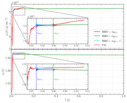
Figure 12: Evolution of the central rest-mass density (top) and of central conformal factor (bottom) as obtained from different evolutions. In particular, the red solid line refers to the FIL simulation carried out till $t=112\,\mathrm{ms}$, the blue solid line shows the BHAC+ evolution with HO at $t_{\mathrm{HO},1}$, while the green solid line shows the BHAC+ evolution with HO at $t_{\mathrm{HO},2}$ and continued till $t=1000\,\mathrm{ms}$. Also shown with a light-blue solid line is the BHAC+ evolution with HO at $t_{\mathrm{HO},1}$ but with a rescaling of the conformal factor $\tilde{\psi}=1.00038\,\psi$ to account for the slightly different spacetimes in FIL and BHAC+.

We conclude this section on the long-term evolution of a post-merger remnant by presenting in Fig. 12 a much more precise comparison between the different evolutions. In particular, we report in Fig. 12 the evolution of the maximum values of the rest-mass density $\rho_{c}$ (top part) and of the conformal factor $\psi_{c}$ (bottom part). Note that, as done so far in other figures, we show with red solid lines the evolutions coming from FIL , while we indicate with either a blue or a green solid line the evolutions from BHAC+ with HOs at $t_{\mathrm{HO},1}$ and $t_{\mathrm{HO},2}$, respectively.

The first piece of information that can be readily appreciated from Fig. 12 is that the differences in the evolution of the two quantities are of the order of $\sim 1-2\%$ over the whole timescale in which the FIL evolution is carried out, i.e., $\bar{t}=100\,{\rm ms}$ (see insets). Hence, this figure provides a strong and reassuring evidence that the use of the CFC approximation does not yield to large quantitative differences in either the gravitational fields or the matter variables even in the regions of strongest curvature. The second piece of information is also quite self-evident: the central rest-mass density and the conformal factor grow linearly with time in the FIL evolution, while they remain essentially constant in the evolutions with BHAC+ (in practice the central rest-mass density increases of $+1.8\%$ from $\bar{t}=t_{\mathrm{HO},2}$ to $1~{}\mathrm{s}$) This is not surprising and reflects the fact that the emission of GWs in FIL, and the consequent loss of energy and angular momentum in the remnant, leads to an increase of its compactness and hence of the central rest-mass density and conformal factor Baiotti et al. (2008). Since these losses are neglected in the present implementation of the xCFC equations, the evolutions with BHAC+ can only show a slight increase in the central rest-mass density, as shown by blue and green solid lines.

The third and final piece of information in Fig. 12 comes from noting that while the differences in the evolutions with FIL and BHAC+ are minute and much smaller than the uncertainties that accompany the evolution of the post-merger remnant when all the physical and microphysical effects are taken into account, these differences can be reduced through a simple but artificial rescaling of the conformal factor at $t_{\mathrm{HO},1}$. In particular, the inset in the bottom panel of Fig. 12 reveals that the value of $\psi_{c}$ at HO drops by a factor $\sim 0.1\%$ (compare red and blue solid lines) as a result of the mismatch between the different descriptions of the spacetime in the two codes. This mismatch, however, can be easily compensated by a global rescaling of the conformal factor by a constant coefficient $1.00038$ and is shown by the evolutions indicated with light-blue solid lines. When comparing these lines with the corresponding evolutions without the rescaling (blue solid lines) it becomes apparent that the match with FIL can be easily improved, albeit rather artificially.

As a concluding remark, we note that while the differences in the FIL and BHAC+ evolutions of the post-merger remnant are of the order of a couple of percent, the corresponding computational costs differ by a factor $\sim 65$. In particular, while the evolution in FIL between the HO time $t_{\mathrm{HO},2}$ and the end of the simulation at $\bar{t}=100\,\mathrm{ms}$ implied a computational cost of $\sim 2.75\times 10^{5}$ CPU hours, the same evolution with BHAC+ incurred in $\sim 4.25\times 10^{3}$ CPU hours. Furthermore, the whole computational cost in BHAC+ from $t_{\mathrm{HO},2}$ till the end of the simulation at $\bar{t}=1000\,\mathrm{ms}$ corresponded to $\sim 8.59\times 10^{4}$ CPU hours; assuming a stable remnant, an evolution to one second with FIL would have corresponded to a computational cost of $\sim 5.8\times 10^{6}$ CPU hours, thus making it prohibitive if employed for a large number of binaries.

Finally, as mentioned in Sec. III.2, the computational costs relative to BHAC+ can be further and easily be reduced by a factor $2-3$ if less frequent solutions of the CFC equations are performed; in the comparison presented above, in fact, we have solved the CFC equations with the same frequency as the matter evolution and hence with a spacetime slicing that is similar to that in FIL. On the other hand, this was not strictly necessary and the top panel of Fig. 13 reports the BHAC+ post-merger evolution from from $t_{\mathrm{HO},2}$ till the end of the simulation at $\bar{t}=1000\,\mathrm{ms}$ when using $\xi_{\rm eff}=1,1/3$ and $1/10$ (solid green, dashed blue and dotted cyan lines, respectively). Clearly, the three evolutions are extremely similar and the differences reported in the bottom part of Fig. 13 are always $\lesssim 0.01\%$ even in the extreme case of $\xi_{\rm eff}=1/10$. When exploiting this additional speed-up, it is clear that the computational costs at this resolution can be decreased by a factor $2.1$ and $3.6$ for $\xi_{\rm eff}=1/3$ and $1/10$, respectively. As a result, the 2D BHAC+ simulation with $\xi_{\rm eff}=1/10$ has an effective gain over the corresponding 3D simulation in FIL of a factor $\simeq 230$. This computational saving can only increase when considering higher resolutions and opens the way to the systematic study in 2D of the secular matter and electromagnetic emission from binary-merger remnants.

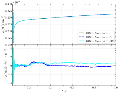
Figure 13: Top panel: Comparison of the evolutions of the central rest-mass density of the BNS remnant when different efficiency ratios are employed. In particular, the top panel reports the evolution with data at $t_{\mathrm{HO},2}$ when $\xi_{\rm eff}=1$ (green solid line; this is the same as in the top panel of Fig. 12), $\xi_{\rm eff}=1/3$ (blue dashed line) and $\xi_{\rm eff}=1/10$ (cyan dotted line). The bottom panel reports instead the relative difference with respect to the $\xi_{\rm eff}=1$ reference evolution (blue and cyan solid lines for $\xi_{\rm eff}=1/3$ and $1/10$, respectively) and shows that the variance is $\lesssim 0.01\%$ even for the most extreme case of $\xi_{\rm eff}=1/10$; the latter simulation was performed with a computational gain of a factor $3.6$ with respect to the corresponding $\xi_{\rm eff}=1$ simulation.

V Conclusions and Outlook

One of the main challenges to be faced when modelling BNS mergers is the accurate long-term evolution of the post-merger remnant over timescales of the order of several seconds. When this modeling is made including all the relevant aspects of the complex physics accompanying the remnant – and which includes the proper treatment of magnetic fields, of realistic EOSs, and of neutrino transport – the computational costs can easily become enormous. To address this challenge in part, we have developed a novel hybrid approach that couples the full numerical-relativity GRMHD code FIL Most et al. (2019a) with the versatile, multi-coordinate and multi-dimensional GRMHD code BHAC, which possesses robust divergence-cleaning methods Porth et al. (2017) and constraint-transport methods Olivares et al. (2019) for the enforcement of the divergence-free condition of the magnetic field. However, because BHAC was developed to solve the equations of GRMHD on arbitrarily curved but fixed spacetimes, we have extended the code capabilities by constructing BHAC+, which employs the CFC approximation of the Einstein equations. More specifically, by assuming a locally flat conformal metric, such an approximation simplifies the Einstein equations reducing them to a set of elliptic equations that can be solved to compute the evolution of the spacetime as a response to the changes in the energy-momentum tensor. A number of applications in core-collapse simulations, but also in the study of merging neutron-star binaries, have shown that the CFC approximation achieves good agreement with full general-relativistic simulations, especially in isolated systems with axisymmetry. The most important advantage of the CFC approximation is however that the corresponding elliptic equations need to solved only every $3-100$ steps of the underlying hydrodynamical/magnetohydrodynamical evolution, thus allowing to the capture even the highest-frequency modes of a fluid compact object at a fraction of the computational cost.

We have therefore presented in detail the basic features of the new code BHAC+, illustrating both the numerical setup for the solution of the Einstein and GRMHD equations, and the strategies necessary to interface BHAC+ with a fully general-relativistic code, such as FIL, when importing both 2D and 3D data. Furthermore, we have methodically described our implementation of an efficient and reliable primitive-recovery scheme coupled with a finite-temperature and tabulated EOS, demonstrating not only its robustness under a large variety of physical regimes, but also its efficiency, which is comparable to (if not higher than) the best reported in the literature so far.

In addition to describing our new methodology, we have also shown the results of a series of standard and non-standard benchmark tests that have been carried out to validate the various parts of the code. These tests have been carried out with various coordinates systems and different numbers of spatial dimensions, from 1D to fully 3D simulations, and for timescales ranging from $5$ to $1000$ milliseconds. More specifically, our tests have considered the simulation of oscillating spherical stars with either a fixed or dynamical spacetime, the dynamics of an unstable spherical star migrating over to the branch of stable configurations, the simulation of a differentially rotating star endowed with a strong toroidal magnetic field, as well as the long-term stability of an unmagnetized but rapidly rotating star near the mass-shedding limit. In many of these tests, the evolution carried out with BHAC+ has been compared with the equivalent one carried out with FIL, finding always a very good agreement.

Our list of benchmarks has been completed by two additional and challenging tests. The first one has involved the head-on collision of two equal-mass stars obeying a temperature-dependent EOS, whose dynamics has been compared in detail with the corresponding one obtained with FIL revealing a remarkable agreement despite the very different handling of the spacetime. The second one, instead, has explored in the detail the hand-off procedure of data from FIL to BHAC+ in the 2D long-term evolution of a BNS merger remnant. In particular, we have demonstrated BHAC+’s ability of importing – even at different times – matter and spacetime data from FIL describing the merger remnant and further evolving it for hundreds of milliseconds and up to one second after merger. While the evolution with BHAC+ cannot by construction reproduce the small changes observed in FIL’s remnant as a result of the emission of GWs, the agreement between the two evolutions is very good and below a couple of percent. More importantly, the computational costs between the 3D FIL evolution and the 2D BHAC+ evolution differ by a factor up to $230$ even at the modest resolutions considered here, with the computational gain becoming larger as the resolution is increased. This substantial difference opens the way to a much more systematic exploration of the long-term evolution of post-merger remnants, that is no longer restricted to considering a single specific case, but can include variations in mass, EOS, magnetic-field properties, etc.

Overall, the results presented here provide two main evidences. First, BHAC+ is able to accurately reproduce the evolution of compact objects in non-vacuum spacetimes and the use of the CFC approximation reproduces accurately both the gravitational fields and the matter variables even in the regions of strongest curvature. Second, a hybrid approach in which a short-term but full numerical-relativity treatment of the dynamics of merging binaries is coupled to a long-term but CFC approximation for the evolution of the post-merger remnant has great potential to obtain an accurate description of the secular electromagnetic and matter emission from binary mergers.

At the same time, a number of improvements can to be implemented to achieve an even more accurate and physically realistic description of these scenarios. These include the addition of radiation-reaction terms in the CFC approximation, of the coupling of the GRMHD equations with those of neutrino radiative transfer, and the handling of scenarios of black-hole formation. We will report about these improvements in future works.

Software:

BHAC Porth et al. (2017); Olivares et al. (2019); Ripperda et al. (2019), FIL Most et al. (2019a), ETK Löffler et al. (2012), RNS Stergioulas and Friedman (1995), FUKA Papenfort et al. (2021), XNS Bucciantini and Del Zanna (2011); Pili et al. (2014), StellarCollapse (https://stellarcollapse.org), CompOSE (https://compose.obspm.fr)

References

- The LIGO Scientific Collaboration and The Virgo Collaboration (2017) The LIGO Scientific Collaboration and The Virgo Collaboration (LIGO Scientific Collaboration and Virgo Collaboration), Phys. Rev. Lett. 119, 161101 (2017), arXiv:1710.05832 [gr-qc] .
- Abbott et al. (2017) B. P. Abbott, R. Abbott, T. D. Abbott, F. Acernese, K. Ackley, C. Adams, T. Adams, P. Addesso, R. X. Adhikari, V. B. Adya, and et al. (LIGO Scientific Collaboration and Virgo Collaboration), Phys. Rev. Lett. 119, 161101 (2017), arXiv:1710.05832 [gr-qc] .
- The LIGO Scientific Collaboration et al. (2017) The LIGO Scientific Collaboration, the Virgo Collaboration, B. P. Abbott, R. Abbott, T. D. Abbott, F. Acernese, K. Ackley, C. aAdams, T. Adams, P. Addesso, R. X. Adhikari, V. B. Adya, and et al. (LIGO Scientific Collaboration and Virgo Collaboration), Astrophys. J. Lett. 848, L12 (2017), arXiv:1710.05833 [astro-ph.HE] .
- Rezzolla et al. (2011) L. Rezzolla, B. Giacomazzo, L. Baiotti, J. Granot, C. Kouveliotou, and M. A. Aloy, Astrophys. J. Letters 732, L6 (2011), arXiv:1101.4298 [astro-ph.HE] .
- Just et al. (2016) O. Just, M. Obergaulinger, H.-T. Janka, A. Bauswein, and N. Schwarz, Astrophys. J. Lett. 816, L30 (2016), arXiv:1510.04288 [astro-ph.HE] .
- Ciolfi (2020) R. Ciolfi, Monthly Notices of the Royal Astronomical Society: Letters 495, L66–L70 (2020).
- Hayashi et al. (2022) K. Hayashi, S. Fujibayashi, K. Kiuchi, K. Kyutoku, Y. Sekiguchi, and M. Shibata, Phys. Rev. D 106, 023008 (2022), arXiv:2111.04621 [astro-ph.HE] .
- Metzger et al. (2010) B. D. Metzger, G. Martínez-Pinedo, S. Darbha, E. Quataert, A. Arcones, D. Kasen, R. Thomas, P. Nugent, I. V. Panov, and N. T. Zinner, Mon. Not. R. Astron. Soc. 406, 2650 (2010), arXiv:1001.5029 [astro-ph.HE] .
- Bovard et al. (2017) L. Bovard, D. Martin, F. Guercilena, A. Arcones, L. Rezzolla, and O. Korobkin, Phys. Rev. D 96, 124005 (2017), arXiv:1709.09630 [gr-qc] .
- Smartt and Chen (2017) S. Smartt and T. e. a. Chen, Nature 551, 75 (2017), arXiv:1710.05841 .
- Papenfort et al. (2018) L. J. Papenfort, R. Gold, and L. Rezzolla, Phys. Rev. D 98, 104028 (2018), arXiv:1807.03795 [gr-qc] .
- Combi and Siegel (2023a) L. Combi and D. M. Siegel, Astrophys. J. 944, 28 (2023a), arXiv:2206.03618 [astro-ph.HE] .
- Fujibayashi et al. (2023) S. Fujibayashi, K. Kiuchi, S. Wanajo, K. Kyutoku, Y. Sekiguchi, and M. Shibata, Astrophys. J. 942, 39 (2023), arXiv:2205.05557 [astro-ph.HE] .
- Kawaguchi et al. (2023) K. Kawaguchi, S. Fujibayashi, N. Domoto, K. Kiuchi, M. Shibata, and S. Wanajo, arXiv preprint arXiv:2306.06961 (2023).
- Baiotti and Rezzolla (2017) L. Baiotti and L. Rezzolla, Rept. Prog. Phys. 80, 096901 (2017), arXiv:1607.03540 [gr-qc] .
- Paschalidis (2017) V. Paschalidis, Classical and Quantum Gravity 34, 084002 (2017), arXiv:1611.01519 [astro-ph.HE] .
- Rezzolla et al. (2018) L. Rezzolla, P. Pizzochero, D. I. Jones, N. Rea, and I. Vidaña, The Physics and Astrophysics of Neutron Stars, Vol. 457 (2018).
- Li et al. (2018) B. Li, L.-B. Li, Y.-F. Huang, J.-J. Geng, Y.-B. Yu, and L.-M. Song, Astrophys. J. Letters 859, L3 (2018), arXiv:1802.10397 [astro-ph.HE] .
- Metzger et al. (2018) B. D. Metzger, T. A. Thompson, and E. Quataert, Astrophys. J. 856, 101 (2018), arXiv:1801.04286 [astro-ph.HE] .
- Nedora et al. (2019) V. Nedora, S. Bernuzzi, D. Radice, A. Perego, A. Endrizzi, and N. Ortiz, Astrophys. J. Lett. 886, L30 (2019), arXiv:1907.04872 [astro-ph.HE] .
- Combi and Siegel (2023b) L. Combi and D. M. Siegel, arXiv e-prints , arXiv:2303.12284 (2023b), arXiv:2303.12284 [astro-ph.HE] .
- Pavan et al. (2021) A. Pavan, R. Ciolfi, J. V. Kalinani, and A. Mignone, Monthly Notices of the Royal Astronomical Society 506, 3483 (2021).
- Kiuchi et al. (2022) K. Kiuchi, S. Fujibayashi, K. Hayashi, K. Kyutoku, Y. Sekiguchi, and M. Shibata, arXiv e-prints , arXiv:2211.07637 (2022), arXiv:2211.07637 [astro-ph.HE] .
- Pais et al. (2022) M. Pais, T. Piran, Y. Lyubarsky, K. Kiuchi, and M. Shibata, arXiv preprint arXiv:2211.09135 (2022).
- Giacomazzo et al. (2009) B. Giacomazzo, L. Rezzolla, and L. Baiotti, Mon. Not. R. Astron. Soc. 399, L164 (2009), arXiv:0901.2722 [gr-qc] .
- Kiuchi et al. (2014) K. Kiuchi, K. Kyutoku, Y. Sekiguchi, M. Shibata, and T. Wada, Phys. Rev. D 90, 041502 (2014), arXiv:1407.2660 [astro-ph.HE] .
- Carrasco et al. (2020) F. Carrasco, D. Viganò, and C. Palenzuela, Phys. Rev. D 101, 063003 (2020), arXiv:1908.01419 [astro-ph.HE] .
- Chabanov et al. (2023) M. Chabanov, S. D. Tootle, E. R. Most, and L. Rezzolla, Astrophys. J. Lett. 945, L14 (2023), arXiv:2211.13661 [astro-ph.HE] .
- Dimmelmeier et al. (2002a) H. Dimmelmeier, J. A. Font, and E. Müller, Astron. Astrophys. 388, 917 (2002a).
- Cordero-Carrión et al. (2009) I. Cordero-Carrión, P. Cerdá-Durán, H. Dimmelmeier, J. L. Jaramillo, J. Novak, and E. Gourgoulhon, Phys. Rev. D 79, 024017 (2009), arXiv:0809.2325 [gr-qc] .
- Cheong et al. (2020) P. C.-K. Cheong, L.-M. Lin, and T. G. F. Li, Classical and Quantum Gravity 37, 145015 (2020).
- Yip et al. (2023) A. K. L. Yip, P. C.-K. Cheong, and T. G. F. Li, arXiv preprint arXiv:2303.16820 (2023).
- Dimmelmeier et al. (2002b) H. Dimmelmeier, J. A. Font, and E. Müller, Astron. Astrophys. 393, 523 (2002b).
- Ott et al. (2007) C. D. Ott, H. Dimmelmeier, A. Marek, H. Janka, B. Zink, I. Hawke, and E. Schnetter, Class. Quantum Grav. 24, 139 (2007), arXiv:astro-ph/0612638 .
- Müller (2015) B. Müller, Monthly Notices of the Royal Astronomical Society 453, 287 (2015).
- Cheong et al. (2021) P. C.-K. Cheong, A. T.-L. Lam, H. H.-Y. Ng, and T. G. F. Li, Monthly Notices of the Royal Astronomical Society 508, 2279 (2021), https://academic.oup.com/mnras/article-pdf/508/2/2279/40566816/stab2606.pdf .
- Bauswein et al. (2012) A. Bauswein, H.-T. Janka, K. Hebeler, and A. Schwenk, Phys. Rev. D 86, 063001 (2012), arXiv:1204.1888 [astro-ph.SR] .
- Bauswein et al. (2021) A. Bauswein, S. Blacker, G. Lioutas, T. Soultanis, V. Vijayan, and N. Stergioulas, Phys. Rev. D 103, 123004 (2021), arXiv:2010.04461 [astro-ph.HE] .
- Lioutas et al. (2022) G. Lioutas, A. Bauswein, T. Soultanis, R. Pakmor, V. Springel, and F. K. Röpke, arXiv preprint arXiv:2208.04267 (2022).
- Blacker et al. (2023) S. Blacker, H. Kochankovski, A. Bauswein, A. Ramos, and L. Tolos, arXiv preprint arXiv:2307.03710 (2023).
- Kastaun and Galeazzi (2015) W. Kastaun and F. Galeazzi, Phys. Rev. D 91, 064027 (2015), arXiv:1411.7975 [gr-qc] .
- Hanauske et al. (2017) M. Hanauske, K. Takami, L. Bovard, L. Rezzolla, J. A. Font, F. Galeazzi, and H. Stöcker, Phys. Rev. D 96, 043004 (2017), arXiv:1611.07152 [gr-qc] .
- Most et al. (2019a) E. R. Most, L. J. Papenfort, and L. Rezzolla, Mon. Not. R. Astron. Soc. 490, 3588 (2019a), arXiv:1907.10328 [astro-ph.HE] .
- Most et al. (2021) E. R. Most, L. J. Papenfort, S. D. Tootle, and L. Rezzolla, Astrophys. J. 912, 80 (2021), arXiv:2012.03896 [astro-ph.HE] .
- Porth et al. (2017) O. Porth, H. Olivares, Y. Mizuno, Z. Younsi, L. Rezzolla, M. Moscibrodzka, H. Falcke, and M. Kramer, Computational Astrophysics and Cosmology 4, 1 (2017), arXiv:1611.09720 [gr-qc] .
- Olivares et al. (2019) H. Olivares, O. Porth, J. Davelaar, E. R. Most, C. M. Fromm, Y. Mizuno, Z. Younsi, and L. Rezzolla, Astron. Astrophys. 629, A61 (2019).
- Ripperda et al. (2019) B. Ripperda, F. Bacchini, O. Porth, E. R. Most, H. Olivares, A. Nathanail, L. Rezzolla, J. Teunissen, and R. Keppens, Astrophys. J., Supp. 244, 10 (2019), arXiv:1907.07197 [physics.comp-ph] .
- Porth et al. (2019) O. Porth, K. Chatterjee, and Event Horizon Telescope Collaboration, Astrophys. J. Supp. 243, 26 (2019), arXiv:1904.04923 [astro-ph.HE] .
- Shibata and Nakamura (1995) M. Shibata and T. Nakamura, Phys. Rev. D 52, 5428 (1995).
- Baumgarte and Shapiro (1999) T. W. Baumgarte and S. L. Shapiro, Phys. Rev. D 59, 024007 (1999), gr-qc/9810065 .
- Alic et al. (2012) D. Alic, C. Bona-Casas, C. Bona, L. Rezzolla, and C. Palenzuela, Phys. Rev. D 85, 064040 (2012), arXiv:1106.2254 [gr-qc] .
- Alic et al. (2013) D. Alic, W. Kastaun, and L. Rezzolla, Phys. Rev. D 88, 064049 (2013), arXiv:1307.7391 [gr-qc] .
- Bernuzzi and Hilditch (2010) S. Bernuzzi and D. Hilditch, Phys. Rev. D 81, 084003 (2010), arXiv:0912.2920 [gr-qc] .
- York (1971) J. W. York, Phys. Rev. Lett. 26, 1656 (1971).
- Cook et al. (1996) G. B. Cook, S. L. Shapiro, and S. A. Teukolsky, Physical Review D 53, 5533 (1996).
- Dimmelmeier et al. (2006) H. Dimmelmeier, N. Stergioulas, and J. A. Font, Mon. Not. R. Astron. Soc. 368, 1609 (2006), arXiv:astro-ph/0511394 .
- Alcubierre (2006) M. Alcubierre, Introduction to 3+1 Numerical Relativity (2006), 10.1093/acprof:oso/9780199205677.001.0001.
- Rezzolla and Zanotti (2013) L. Rezzolla and O. Zanotti, Relativistic Hydrodynamics (Oxford University Press, Oxford, UK, 2013).
- Bucciantini and Del Zanna (2011) N. Bucciantini and L. Del Zanna, Astron. Astrophys. 528, A101 (2011), arXiv:1010.3532 [astro-ph.IM] .
- Ng et al. (2021) H. H.-Y. Ng, P. C.-K. Cheong, L.-M. Lin, and T. G. F. Li, The Astrophysical Journal 915, 108 (2021), arXiv:2012.08263 [astro-ph.HE] .
- Leung et al. (2022) M. Y. Leung, A. K. L. Yip, P. C.-K. Cheong, and T. G. F. Li, Communications Physics 5, 334 (2022).
- Cheong et al. (2022) P. C.-K. Cheong, D. Y. T. Pong, A. K. L. Yip, and T. G. F. Li, Astrophys. J. Suppl. 261 (2022), 10.3847/1538-4365/ac6cec.
- Servignat et al. (2023) G. Servignat, J. Novak, and I. Cordero-Carrión, Classical and Quantum Gravity 40, 105002 (2023).
- Cheong et al. (2023) P. C.-K. Cheong, H. H.-Y. Ng, A. T.-L. Lam, and T. G. F. Li, The Astrophysical Journal Supplement Series 267, 38 (2023).
- Faye and Schäfer (2003) G. Faye and G. Schäfer, Physical Review D 68, 084001 (2003).
- Oechslin et al. (2007) R. Oechslin, H.-T. Janka, and A. Marek, Astron. Astrophys. 467, 395 (2007), astro-ph/0611047 .
- Jiang et al. (2024) J.-L. Jiang, H. H.-Y. Ng, M. Chabanov, and L. Rezzolla, (2024), in preparation.
- Papenfort et al. (2021) L. J. Papenfort, S. D. Tootle, P. Grandclément, E. R. Most, and L. Rezzolla, arXiv e-prints , arXiv:2103.09911 (2021), arXiv:2103.09911 [gr-qc] .
- Tootle et al. (2022) S. Tootle, C. Ecker, K. Topolski, T. Demircik, M. Järvinen, and L. Rezzolla, SciPost Phys. 13, 109 (2022), arXiv:2205.05691 [astro-ph.HE] .
- (70) LORENE, “Langage objet pour la relativité numérique,” Langage Objet pour la RElativité Numérique, www.lorene.obspm.fr.
- Tsokaros et al. (2015) A. Tsokaros, K. Uryū, and L. Rezzolla, Phys. Rev. D 91, 104030 (2015), arXiv:1502.05674 [gr-qc] .
- Most et al. (2019b) E. R. Most, L. J. Papenfort, A. Tsokaros, and L. Rezzolla, Astrophys. J. 884, 40 (2019b), arXiv:1904.04220 [astro-ph.HE] .
- Loeffler et al. (2012) F. Loeffler, J. Faber, E. Bentivegna, T. Bode, P. Diener, R. Haas, I. Hinder, B. C. Mundim, C. D. Ott, E. Schnetter, G. Allen, M. Campanelli, and P. Laguna, Class. Quantum Grav. 29, 115001 (2012), arXiv:1111.3344 [gr-qc] .
- Zlochower and et al. (2022) Y. Zlochower and et al., “The einstein toolkit,” (2022), to find out more, visit http://einsteintoolkit.org.
- Schnetter et al. (2006) E. Schnetter, P. Diener, E. N. Dorband, and M. Tiglio, Class. Quantum Grav. 23, S553 (2006), arXiv:gr-qc/0602104 .
- Teunissen and Keppens (2019) J. Teunissen and R. Keppens, Computer Physics Communications 245, 106866 (2019).
- Porth et al. (2014) O. Porth, C. Xia, T. Hendrix, S. P. Moschou, and R. Keppens, Astrophys. J., Supp. 214, 4 (2014), arXiv:1407.2052 [astro-ph.IM] .
- Toro (1999) E. F. Toro, Riemann Solvers and Numerical Methods for Fluid Dynamics (Springer-Verlag, 1999).
- Etienne et al. (2015) Z. B. Etienne, V. Paschalidis, R. Haas, P. Mösta, and S. L. Shapiro, Class. Quantum Grav. 32, 175009 (2015), arXiv:1501.07276 [astro-ph.HE] .
- Del Zanna et al. (2007) L. Del Zanna, O. Zanotti, N. Bucciantini, and P. Londrillo, Astron. Astrophys. 473, 11 (2007), arXiv:0704.3206 .
- Mizuno et al. (2018) Y. Mizuno, Z. Younsi, C. M. Fromm, O. Porth, M. De Laurentis, H. Olivares, H. Falcke, M. Kramer, and L. Rezzolla, Nature Astronomy 2, 585 (2018), arXiv:1804.05812 [astro-ph.GA] .
- Olivares et al. (2020) H. Olivares, Z. Younsi, C. M. Fromm, M. De Laurentis, O. Porth, Y. Mizuno, H. Falcke, M. Kramer, and L. Rezzolla, MNRAS 497, 521 (2020), arXiv:1809.08682 [gr-qc] .
- Cruz-Osorio et al. (2023) A. Cruz-Osorio, L. Rezzolla, F. D. Lora-Clavijo, J. A. Font, C. Herdeiro, and E. Radu, Journal of Cosmology and Astroparticle Physics 2023, 057 (2023), arXiv:2301.06564 [astro-ph.HE] .
- Cruz-Osorio et al. (2022) A. Cruz-Osorio, C. M. Fromm, Y. Mizuno, A. Nathanail, Z. Younsi, O. Porth, J. Davelaar, H. Falcke, M. Kramer, and L. Rezzolla, Nature Astronomy 6, 103 (2022), arXiv:2111.02517 [astro-ph.HE] .
- Das et al. (2022) P. Das, O. Porth, and A. L. Watts, Monthly Notices of the Royal Astronomical Society 515, 3144 (2022), arXiv:2204.00249 [astro-ph.HE] .
- Çıkıntoğlu et al. (2022) S. Çıkıntoğlu, K. Y. Ekşi, and L. Rezzolla, Mon. Not. R. Astron. Soc. 517, 3212 (2022), arXiv:2204.12275 [astro-ph.HE] .
- Chabanov et al. (2021) M. Chabanov, L. Rezzolla, and D. H. Rischke, Mon. Not. R. Astron. Soc. 505, 5910 (2021), arXiv:2102.10419 [gr-qc] .
- Londrillo and Del Zanna (2004) P. Londrillo and L. Del Zanna, Journal of Computational Physics 195, 17 (2004).
- Evans and Hawley (1988) C. R. Evans and J. F. Hawley, Astrophys. J. 332, 659 (1988).
- Banyuls et al. (1997) F. Banyuls, J. A. Font, J. M. Ibáñez, J. M. Martí, and J. A. Miralles, Astrophys. J. 476, 221 (1997).
- Galeazzi et al. (2013) F. Galeazzi, W. Kastaun, L. Rezzolla, and J. A. Font, Phys. Rev. D 88, 064009 (2013), arXiv:1306.4953 [gr-qc] .
- Palenzuela et al. (2015) C. Palenzuela, S. L. Liebling, D. Neilsen, L. Lehner, O. L. Caballero, E. O’Connor, and M. Anderson, Phys. Rev. D 92, 044045 (2015), arXiv:1505.01607 [gr-qc] .
- (93) Stellar Collapse Repository, (2017), https://stellarcollapse.org.
- Typel et al. (2015) S. Typel, M. Oertel, and T. Klähn, Physics of Particles and Nuclei 46, 633 (2015).
- Siegel et al. (2018) D. M. Siegel, P. Mösta, D. Desai, and S. Wu, Astrophys. J. 859, 71 (2018), arXiv:1712.07538 [astro-ph.HE] .
- Espino et al. (2022) P. L. Espino, G. Bozzola, and V. Paschalidis, arXiv e-prints , arXiv (2022).
- Kastaun et al. (2021) W. Kastaun, J. V. Kalinani, and R. Ciolfi, Physical Review D 103, 023018 (2021).
- Ng et al. (2023) H. H.-Y. Ng, P. C.-K. Cheong, A. T.-L. Lam, and T. G. F. Li, (2023), arXiv:2309.03526 [astro-ph.HE] .
- Löffler et al. (2012) F. Löffler, J. Faber, E. Bentivegna, T. Bode, P. Diener, R. Haas, I. Hinder, B. C. Mundim, C. D. Ott, E. Schnetter, G. Allen, M. Campanelli, and P. Laguna, Class. Quantum Grav. 29, 115001 (2012), arXiv:1111.3344 [gr-qc] .
- Brent (2002) R. P. Brent, Algorithms for Minimization Without Derivatives, reprinted ed. (Dover, New York, 2002).
- Lattimer and Swesty (1991) J. M. Lattimer and F. D. Swesty, Nucl. Phys. A 535, 331 (1991).
- Neilsen et al. (2014) D. W. Neilsen, S. L. Liebling, M. Anderson, L. Lehner, E. O’Connor, and C. Palenzuela, Phys. Rev. D 89, 104029 (2014), arXiv:1403.3680 [gr-qc] .
- Newman and Hamlin (2014) W. Newman and N. Hamlin, SIAM Journal on Scientific Computing 36, B661 (2014), https://doi.org/10.1137/140956749 .
- Noble et al. (2006) S. C. Noble, C. F. Gammie, J. C. McKinney, and L. Del Zanna, Astrophys. J. 641, 626 (2006), astro-ph/0512420 .
- Antón et al. (2006) L. Antón, O. Zanotti, J. A. Miralles, J. M. Martí, J. M. Ibáñez, J. A. Font, and J. A. Pons, Astrophys. J. 637, 296 (2006), astro-ph/0506063 .
- Cerdá-Durán et al. (2008) P. Cerdá-Durán, J. A. Font, L. Antón, and E. Müller, Astron. Astrophys. 492, 937 (2008), arXiv:0804.4572 .
- Harten et al. (1983) A. Harten, P. D. Lax, and B. van Leer, SIAM Rev. 25, 35 (1983).
- Einfeldt (1988) B. Einfeldt, SIAM J. Numer. Anal. 25, 294 (1988).
- Borges et al. (2008) R. Borges, M. Carmona, B. Costa, and W. Don, Journal of Computational Physics 227, 3191 (2008).
- Colella and Woodward (1984) P. Colella and P. R. Woodward, Journal of Computational Physics 54, 174 (1984).
- Löhner (1987) R. Löhner, Computer Methods in Applied Mechanics and Engineering 61, 323 (1987).
- Font et al. (2002) J. A. Font, T. Goodale, S. Iyer, M. Miller, L. Rezzolla, E. Seidel, N. Stergioulas, W.-M. Suen, and M. Tobias, Phys. Rev. D 65, 084024 (2002), gr-qc/0110047 .
- Stergioulas et al. (2004) N. Stergioulas, T. A. Apostolatos, and J. A. Font, Mon. Not. R. Astron. Soc. 352, 1089 (2004), arXiv:astro-ph/0312648 .
- Pili et al. (2014) A. G. Pili, N. Bucciantini, and L. Del Zanna, Mon. Not. R. Astron. Soc. 439, 3541 (2014), arXiv:1401.4308 [astro-ph.HE] .
- Radice et al. (2014) D. Radice, L. Rezzolla, and F. Galeazzi, Class. Quantum Grav. 31, 075012 (2014), arXiv:1312.5004 [gr-qc] .
- Cerdá-Durán (2010) P. Cerdá-Durán, Classical and Quantum Gravity 27, 205012 (2010), arXiv:0912.1774 [astro-ph.SR] .
- Chabanov and Rezzolla (2023) M. Chabanov and L. Rezzolla, arXiv e-prints , arXiv:2307.10464 (2023), arXiv:2307.10464 [gr-qc] .
- Komatsu et al. (1989) H. Komatsu, Y. Eriguchi, and I. Hachisu, Mon. Not. R. Astron. Soc. 239, 153 (1989).
- Kiuchi and Yoshida (2008) K. Kiuchi and S. Yoshida, Phys. Rev. D 78, 044045 (2008), arXiv:0802.2983 .
- Hempel and Schaffner-Bielich (2010) M. Hempel and J. Schaffner-Bielich, Nuclear Physics A 837, 210 (2010), arXiv:0911.4073 [nucl-th] .
- Stergioulas and Friedman (1995) N. Stergioulas and J. L. Friedman, Astrophys. J. 444, 306 (1995), astro-ph/9411032 .
- Musolino and Rezzolla (2023) C. Musolino and L. Rezzolla, arXiv e-prints , arXiv:2304.09168 (2023), arXiv:2304.09168 [gr-qc] .
- Kellerman et al. (2010) T. Kellerman, L. Rezzolla, and D. Radice, Class. Quantum Grav. 27, 235016 (2010), arXiv:1007.2797 [gr-qc] .
- East and Pretorius (2013) W. E. East and F. Pretorius, Phys. Rev. Lett. 110, 101101 (2013), arXiv:1210.0443 [gr-qc] .
- Rezzolla and Takami (2013) L. Rezzolla and K. Takami, Class. Quantum Grav. 30, 012001 (2013), arXiv:1209.6138 [gr-qc] .
- Grandclement (2010) P. Grandclement, J. Comput. Phys. 229, 3334 (2010), arXiv:0909.1228 [gr-qc] .
- Papenfort et al. (2021) L. J. Papenfort, S. D. Tootle, P. Grandclément, E. R. Most, and L. Rezzolla, Phys. Rev. D 104, 024057 (2021).
- Tootle (2023) S. Tootle, Probing extreme configurations in binary compact object mergers, doctoralthesis, Universitätsbibliothek Johann Christian Senckenberg (2023).
- Pfeiffer and York (2005) H. P. Pfeiffer and J. W. York, Phys. Rev. Lett. 95, 091101 (2005), arXiv:gr-qc/0504142 [gr-qc] .
- Tootle and Rezzolla (2024) S. Tootle and L. Rezzolla, in preparation (2024), arXiv:in preparation .
- Helfer et al. (2022) T. Helfer, U. Sperhake, R. Croft, M. Radia, B.-X. Ge, and E. A. Lim, Class. Quant. Grav. 39, 074001 (2022), arXiv:2108.11995 [gr-qc] .
- Lovelace et al. (2008) G. Lovelace, R. Owen, H. P. Pfeiffer, and T. Chu, Phys. Rev. D 78, 084017 (2008), arXiv:0805.4192 [gr-qc] .
- Foucart et al. (2008) F. Foucart, L. E. Kidder, H. P. Pfeiffer, and S. A. Teukolsky, Phys. Rev. D 77, 124051 (2008), arXiv:0804.3787 [gr-qc] .
- Tichy et al. (2019) W. Tichy, A. Rashti, T. Dietrich, R. Dudi, and B. Brügmann, Phys. Rev. D 100, 124046 (2019), arXiv:1910.09690 [gr-qc] .
- Radice and Rezzolla (2012) D. Radice and L. Rezzolla, Astron. Astrophys. 547, A26 (2012), arXiv:1206.6502 [astro-ph.IM] .
- Guercilena et al. (2017) F. Guercilena, D. Radice, and L. Rezzolla, Computational Astrophysics and Cosmology 4, 3 (2017).
- Fujibayashi et al. (2017) S. Fujibayashi, Y. Sekiguchi, K. Kiuchi, and M. Shibata, ArXiv e-prints (2017), arXiv:1703.10191 [astro-ph.HE] .
- Baiotti et al. (2008) L. Baiotti, B. Giacomazzo, and L. Rezzolla, Phys. Rev. D 78, 084033 (2008), arXiv:0804.0594 [gr-qc] .