Supplementary Material

Contents

S1 Illustration Under- or Over-ConfidenceS1
S2 Implementation and Training DetailsS2
S3 Additional ExperimentsS3
– S3.1 Experiment 1: Additional Results on COMPASS3.1
– S3.2 Experiment 1: Analysis on D-VlogS3.2
– S3.3 Experiment 3: Individual Fairness Analysis on Adult2
– S3.4 Experiment 4: Ablation AnalysisS3.4
S4 Limitations and Future WorkS4
ReferencesS4

S1 Illustration of Under- or Over-Confidence

It is well-known that ML models are generally under- or over-confident (guo2017calibration; FocalLoss_Calibration) or unreliable under noise (kendall2017uncertainties). To illustrate that this may also be the case in datasets which are commonly used in fairness analysis, we have plotted the prediction confidence of the BNN classifier on the COMPAS dataset in Fig. S1. The plot shows that the model is under or over-confident abouts its predictions and that there is a so-called calibration gap.

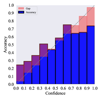
Figure S1: Illustration of Under- or Over-Confidence: An example illustrating under- or over-confidence of an ML model’s predictions. The diagram is calculated for a Bayesian NN classifier on the COMPAS Dataset, a dataset frequently used in fairness in AI.

S2 Implementation and Training Details

For all of our experiments, except for D-Vlog, we utilize Bayesian Neural Networks (BNNs) for both classification and uncertainty estimation. To address the intractability of $P(Y|X)$, we utilize the well-known Bayes by Backprop method (blundell2015weight) which minimizes the following objective consisting of a KL divergence (kullback1951information) term and a numerically-stable negative log-likelihood term as proposed in (kendall2017uncertainties):

$$\mathcal{L}(\theta)=\sum_{m=1}^{M}\underbrace{[\log q_{\theta}(\omega_{m})-\log P(\omega_{m})}_{\text{KL divergence}}+\lambda\underbrace{\mathcal{L}_{NLL}(\hat{Y},Y)}_{\text{classification loss}}].$$ (S1)

with $\lambda$ being a constant.

Measure	Black ($G_{0}$)	White ($G_{1}$)	Younger than 25 ($G_{0}$)	Between 25-45	Older than 45 ($G_{1}$)	Female ($G_{0}$)	Male ($G_{1}$)
$\uparrow$ Sample Size	3175	2103	1347	3532	1293	1175	4997
[1pt/1pt]     Performance Measures
$\uparrow$ $\mathcal{M}_{Acc}$	0.70	0.68	0.64	0.71	0.75	0.77	0.68
$\uparrow$ $\mathcal{M}_{PPV}$	0.69	0.68	0.64	0.72	0.64	0.70	0.68
$\uparrow$ $\mathcal{M}_{NPV}$	0.72	0.68	0.63	0.70	0.78	0.78	0.68
$\downarrow$ $\mathcal{M}_{FPR}$	0.34	0.10	0.41	0.18	0.12	0.05	0.25
$\downarrow$ $\mathcal{M}_{FNR}$	0.25	0.66	0.32	0.44	0.54	0.67	0.39
$\downarrow$ $\mathcal{\mathcal{U}}_{e}$	0.0006	0.0004	0.0010	0.0005	0.0002	0.0003	0.0006
$\downarrow$ $\mathcal{\mathcal{U}}_{a}$	0.2299	0.1578	0.3459	0.1712	0.1027	0.1599	0.2053
$\downarrow$ $\mathcal{\mathcal{U}}_{p}$	0.2305	0.1583	0.3469	0.1717	0.1029	0.1602	0.2059
[1pt/1pt]     Point-based Fairness Measures
$\mathcal{F}_{SP}$	2.84		2.44			0.31
$\mathcal{F}_{EOpp}$	2.19		1.48			0.54
$\mathcal{F}_{EOdd}$	1.57		2.37			0.40
$\mathcal{F}_{EAcc}$	1.03		0.85			1.13
[1pt/1pt]     Uncertainty-based Fairness Measures (Ours)
$\mathcal{F}_{Epis}$	1.55		4.35			0.50
$\mathcal{F}_{Alea}$	1.46		3.36			0.78
$\mathcal{F}_{Pred}$	1.46		3.37			0.78

Table S1: Experiment 2: The analysis with the COMPAS Recidivism Dataset for race (Black vs. White), age (younger than 25 vs. older than 45) and gender (male vs. female) attributes. Severe values of fairness values ($|\mathcal{F}-1|>0.2$, following (zanna2022bias)) are highlighted.

For all experiments, we use the Adam optimizer (kingma2017adam) and following kwon2020uncertainty, we set $T=10$ (the number of Monte Carlo samples for uncertainty quantification as defined in Section 4.1). Furthermore, following one of the settings provided in (blundell2015weight), we use $10$ Monte Carlo samples to approximate the variational posterior, $q_{\theta}(\omega)$, and sample the initial mean of the posterior from a Gaussian with $\mu=0$ and $\sigma=1$. The $\pi$ value, weighting factor for the prior, is set to $0.5$ and the two $\sigma_{1}$ and $\sigma_{2}$ values for the scaled mixture of Gaussians is set to $0$ and $6$ respectively. We consider $\lambda$ from the BNN training objective to be $2000$. We utilize early stopping to determine the number of training iterations for all experiments. In the following, we describe dataset specific details. In all cases, the hyper-parameters are tuned to avoid overfitting:

Synthetic Datasets:

As the datasets are relatively simple, we observed that BNNs with no hidden layers suffice for all three synthetic datasets. We train all of them for $5$ epochs with a batch size of $8$.

COMPAS Recidivism Dataset:

We employ a BNN with a single hidden layer of size $100$. We train the model for $10$ epochs with a batch size of $256$. Similar to (chouldechova2017fair), we consider fairness with respect to race, gender and age. Due to space constraints, the results on age are provided here in the supplementary material. For the race attribute, we follow (zafar2017fairness) and focus on the fairness gap between black and white subgroups, considering blacks as the minority group, $G_{0}$. For the gender attribute, we designate females as the minority group ($G_{0}$) due to the class imbalance in favor of the male group. For the age attribute, we consider individuals younger than $25$ to be the minority group and individuals older than $45$ as the majority group since our classifier provided the worst result for those younger than 25 and overall best results for those older than $45$. To keep the coverage to a binary setting, we did not consider individuals aged between $25$ and $45$. Extending the measures to such a multi-valued setting is straightforward (xu2020investigating) and left as future work.

Adult Income Dataset:

We employ a BNN with no hidden layers where the intermediate size is $25$. We train the model for $5$ epochs with a batch size of $256$. Although a deeper analysis could be conducted through considering other variables such as marriage status, highest education level, occupation and nationality, for the sake of consistency with the analysis of the other datasets, we limit the experiments to race, gender and age.

D-Vlog Depression Detection Dataset:

D-Vlog samples have significantly larger dimensionality (596s of 136-dim visual and 25-dim acoustic features) compared to COMPAS and Adult, which turned out to be challenging for BNNs. Therefore, we utilize the transformer-based Depression Detector architecture proposed by yoon2022dvlog. For uncertainty estimation, we follow lakshminarayanan2017simple to obtain $T$ predictions with an ensemble of $T$ models and use the same method (Eq. 4.1) as with uncertainty estimation with BNNS. Specifically, instead of performing MC forward passes, we train $T$ different models on the same training set and consider their predictions in the same testing set during the uncertainty quantification process. We choose $T=5$ as existing work indicates that performance tends to peak at that number (havasi2020training).

For all of training configurations, we directly use the setting of yoon2022dvlog with a learning rate of $0.0002$ and a batch size of $32$, optimized for $50$ epochs through the Adam optimizer (kingma2017adam). For the dropout rate, we empirically choose $0.1$ though it was not explicitly provided by the authors in the original work. For more details on the architecture and the relevant training details, we refer the reader to (yoon2022dvlog).

S3 Additional Experiments

This section amends the analysis provided in the main manuscript. Section S3.1 extends the Experiment 1 on COMPAS with respect to the analysis on the age attribute. Section S3.2 provides the results on the D-Vlog dataset. Section S3.3 analyzes individual fairness scores for the Adult dataset, extending the analysis in the main manuscript.

S3.1 Experiment 1: Additional Results on COMPAS

In Table S2, we see the complete table for COMPAS, including the age attribute. Across age, we observe that almost all of the performance metrics are better for those age greater than $45$ compared to the others, with the exception of $\mathcal{M}_{PPV}$ and $\mathcal{M}_{FNR}$. For $\mathcal{M}_{PPV}$, samples with ages between $25-45$ is the best with $\mathcal{M}_{PPV}=0.72$ and for $\mathcal{M}_{FNR}$, samples with ages less than $25$ is the best with $\mathcal{M}_{FNR}=0.32$. As explained within Section 5.5 of the main submission, we compute both the point-based and proposed uncertainty-based measures through considering the subgroup age greater than $45$ as the majority subgroup ($G_{1}$) and the subgroup age less than $25$ as the minority ($G_{0}$).

Across the point-based fairness measures, we observe that all but one of the measures point to unfair predictions, with $\mathcal{F}_{SP}=2.44$, $\mathcal{F}_{Opp}=1.48$ and $\mathcal{F}_{Odd}=2.37$. Similar to the race attribute, $\mathcal{F}_{EAcc}=0.85$ claims fair predictions, with all of the other point-based measures directly implying that the model in question is inclined to unfairly predict the subgroup age less than $25$ as $y=1$, i.e recidivating an offense.

Furthermore, the proposed uncertainty-based fairness measures also show similar results with $\mathcal{F}_{Epis}=4.35$, $\mathcal{F}_{Alea}=3.36$ and $\mathcal{F}_{Pred}=3.37$. A similar conclusion with the race attribute could be arrived here with the $\mathcal{F}_{Epis}=4.35$, i.e the lack of data according to the model behavior is higher for the subgroup age less than $25$ compared to the the subgroup age greater than $45$ even though the dataset actually contains less samples for the latter. Even though we also observe a similar pattern with the race attribute with $\mathcal{F}_{Alea}=3.36$ and $\mathcal{F}_{Pred}=3.37$, the fairness gap in this case is significantly higher. These measures also show that the classification hardness, the noise faced by the model according to its own behavior, is drastically higher for the subgroup age less than $25$.

S3.2 Experiment 1: Analysis on D-Vlog

	Male		Female
	$Y=0$	$Y=1$	$Y=0$	$Y=1$
# Samples	140 (0%)	182 (0%)	2666 (0%)	373 (0%)
Avg. Duration(s)	483	583	587	667
Avg. Truncation(s)	-158	-13	-9	+71

Table S2: Label, duration and sensitive attribute distributions of D-Vlog. Both average durations and average truncated amounts are given in seconds. Absolute value of the entries with negative value in the last row shows the amount of zero padding whereas the positive values directly state the amount of truncation..

Dataset Description

D-Vlog contains visual and acoustic features from Youtube videos of 555 depressed and 406 non-depressed samples belonging to 639 females and 322 males. The authors truncated the videos with longer than $t=596s$ and zero-pad shorter ones. D-Vlog only provides the gender attribute for its samples. We follow the training and testing splits as provided by the authors. We assume that the positive label ($Y=1$) stands for the depressed and vice versa.

D-Vlog Truncation Statistics

Table S2 shows that Female videos are truncated significantly, which leads to loss of information and an increase of uncertainty in predictions.

	Multi-Modal		Audio Only		Visual Only
Measure	F	M	F	M	F	M
$\uparrow$ Sample Size	639	322	639	322	639	322
[1pt/1pt]     Performance Measures
$\uparrow$ $\mathcal{M}_{Acc}$	0.59	0.73	0.63	0.75	0.63	0.66
$\uparrow$ $\mathcal{M}_{PPV}$	0.62	0.78	0.72	0.82	0.65	0.69
$\uparrow$ $\mathcal{M}_{NPV}$	0.54	0.66	0.56	0.66	0.61	0.57
$\downarrow$ $\mathcal{M}_{FPR}$	0.57	0.38	0.29	0.28	0.54	0.61
$\downarrow$ $\mathcal{M}_{FNR}$	0.28	0.20	0.43	0.22	0.23	0.18
$\downarrow$ $\mathcal{U}_{e}$	0.006	0.006	0.022	0.016	0.034	0.035
$\downarrow$ $\mathcal{U}_{a}$	0.45	0.45	0.28	0.22	0.10	0.09
$\downarrow$ $\mathcal{U}_{p}$	0.46	0.46	0.31	0.24	0.14	0.13
[1pt/1pt]     Point-based Fairness Measures
$\mathcal{F}_{SP}$	1.01		0.75		0.91
$\mathcal{F}_{Opp}$	0.89		0.73		0.94
$\mathcal{F}_{Odd}$	1.68		1.40		0.94
$\mathcal{F}_{EAcc}$	0.81		0.84		0.96
[1pt/1pt]     Uncertainty-based Fairness Measures (Ours)
$\mathcal{F}_{Epis}$	1.00		1.38		0.96
$\mathcal{F}_{Alea}$	1.00		1.32		1.11
$\mathcal{F}_{Pred}$	1.00		1.32		1.07

Table S3: Experiment 2: The analysis with D-Vlog. Unfair values are highlighted. F/M: Females/Males. $G_{0}$: Females.

Results

As the dataset owners have explored both multi-modal and uni-modal architectures, we analyze D-Vlog both in a multi-modal and in a uni-modal manner. Table S3.2 provides the experimental results. Both point-based and uncertainty-based fairness measures deem the classifier to be fair (except for $\mathcal{F}_{Odd}$). Uncertainty-based fairness results are especially surprising since the Female group size is twice the size of the Male group. However, we observe that the classifier has high aleatoric uncertainty for both groups.

The results per modality suggest that the audio modality has strong bias against Females since the performance measures are generally lower for Females. This, however, is not coherently captured by point-based measures whereas our uncertainty-based measures consistently highlight the bias. The cause of this bias appears to be the truncation of the videos by the dataset owners: Recordings of Females are significantly longer and therefore, truncated more (see the Suppl. Mat. for detailed statistics). This naturally reduces information useful for the classification task, increasing the uncertainty for females. However, this effect is not observed with the visual modality, one reason for which might be that the classifier is performing poorly for both groups.

S3.3 Experiment 3: Individual Fairness Analysis on Adult

With reference to Figure S2, we see that $\mathcal{F}^{indv}_{\hat{y}}$ for both race and gender are largely similar. This is also true for the the Uncertainty-based individual fairness measures $\mathcal{F}^{indv}_{\mathcal{U}_{a}}$ and $\mathcal{F}^{indv}_{\mathcal{U}_{e}}$. A noteworthy point is that all measures indicate an interesting insight about the positive classes, (“B+”, “W+”, “F+” and “M+”). All of them point towards a perfect consistency score of $\approx 1$. We hypothesise that this is due to the severe class imbalance within the Adult dataset where there is a very small subgroup that belongs to the positive class $Y=1$ thus causing the classifier to memorise and be highly confident about the $\hat{Y}=1$ predictions. This is also supported by the small ( 0.07) FPR reported in Table 4 (the main manuscript) for all groups. We see slightly lower consistency for negative classes in point predictions and aleatoric uncertainty. The high FNR rate for both groups (Table 4 in the main text) suggest that there are more errors with $\hat{Y}=0$ predictions, causing higher inconsistencies for those predictions. Lower consistencies for “F-” and “B-” for epistemic uncertainty suggest more data can be helpful for Female and Black groups, supporting the distribution in Table 3 (the main text).

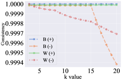
(a) $\mathcal{F}^{indv}_{\hat{y}}$ for race vs $k$

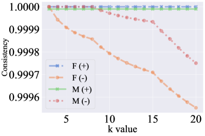
(b) $\mathcal{F}^{indv}_{\hat{y}}$ for gender vs $k$

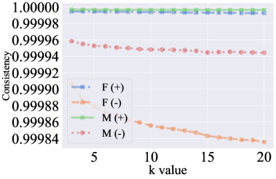
(c) $\mathcal{F}^{indv}_{\mathcal{U}_{a}}$ for gender vs $k$

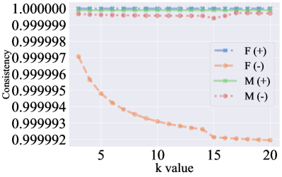
(d) $\mathcal{F}^{indv}_{\mathcal{U}_{e}}$ for gender vs $k$

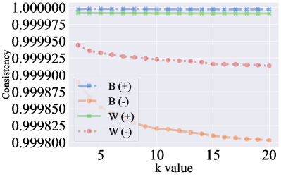
(e) $\mathcal{F}^{indv}_{\mathcal{U}_{a}}$ for race vs $k$

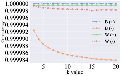
(f) $\mathcal{F}^{indv}_{\mathcal{U}_{e}}$ for race vs $k$

Figure S2: Experiment 3: Point-based (a,b) and uncertainty-based individual fairness (c-f) scores for Adult.

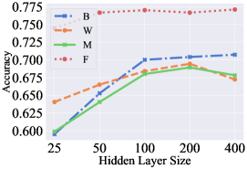
(a) Accuracy

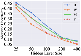
(b) Aleatoric Uncertainty

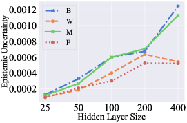
(c) Epistemic Uncertainty

Figure S3: Experiment 4: Ablation analysis on the effect of model capacity on COMPAS. (a) Accuracy. (b) Aleatoric uncertainty. (c) epistemic uncertainty. B/W: Black/White. F/M: Female/Male. As model performance starts saturating at 100 neurons, we have used 100 neurons in BNNs.

S3.4 Experiment 4: Ablation Analysis

We analyze the effect of model capacity on performance and uncertainty estimations. The results in Fig. S3 show that the uncertainty estimations are affected by the change in the number of neurons per layer. However, the relative ordering between the different demographic groups do not appear to be affected. Since accuracy appears to saturate after 100 neurons and to lower the computational cost, we have chosen the hidden layer sizes as 100 in all experiments.

Adding more layers led to significant overfitting problems for SD1, SD2, SD3, COMPAS, and Adult datasets. Therefore, we performed the rest of the experiments with a single hidden-layer for COMPAS and no hidden-layer for SD1, SD2, SD3 and Adult.

S4 Limitations and Future Work

Although prediction uncertainty can be helpful in analyzing fairness, this approach has certain limitations which we view as opportunities for future work. For example, uncertainty estimation requires either using models that directly provide multiple predictions (e.g., BNNs, Deep Ensembles) or modifying models (and their training procedure) to do so (e.g., Monte Carlo Dropout (gal2016dropout)). This hinders the use of state-of-the-art architectures or their trained versions in fairness analysis. Moreover, there is also the overhead involved with obtaining multiple predictions to quantify uncertainty. This can be alleviated with one-pass uncertainty estimation approaches, though they tend to be less reliable than the approaches considered in our paper (abdar2021review).

Quantifying uncertainty in a reliable manner is a challenging and an active research topic (mukhoti2023ddu; liu2020sngp; amersfoort2020duq). Although we have obtained similar outcomes with two different methods (BNNs and Deep Ensembles), we have encountered difficulties with the ranges of estimated uncertainties. It would be beneficial to perform our analyses with newer approaches. Another promising research direction is to consider alternative metrics for measuring the dispersion of uncertainty values in a group as taking the average across a group can miss important characteristics of the distribution.