Optimised Storage for Datalog Reasoning

Abstract

Materialisation facilitates Datalog reasoning by precomputing all consequences of the facts and the rules so that queries can be directly answered over the materialised facts. However, storing all materialised facts may be infeasible in practice, especially when the rules are complex and the given set of facts is large. We observe that for certain combinations of rules, there exist data structures that compactly represent the reasoning result and can be efficiently queried when necessary. In this paper, we present a general framework that allows for the integration of such optimised storage schemes with standard materialisation algorithms. Moreover, we devise optimised storage schemes targeting at transitive rules and union rules, two types of (combination of) rules that commonly occur in practice. Our experimental evaluation shows that our approach significantly improves memory consumption, sometimes by orders of magnitude, while remaining competitive in terms of query answering time.

Introduction

Datalog (Abiteboul, Hull, and Vianu 1995) can describe a domain of interest as a set of “if-then” rules and new facts in this domain can be derived by applying the rules to a set of explicitly given facts until a fixpoint is reached. With the ability to express recursive dependencies, such as transitive closure and graph reachability, Datalog is widely used in different communities. In the Semantic Web community, Datalog is used to capture OWL 2 RL ontologies (Motik et al. 2009) possibly extended with SWRL rules (Horrocks et al. 2004) and can thus be used to answer queries over ontology-enriched data. There are an increasing number of academic and commercial systems that have implemented Datalog, such as LogicBlox (Aref et al. 2015), VLog (Carral et al. 2019), RDFox (Nenov et al. 2015), Vadalog (Bellomarini, Gottlob, and Sallinger 2018), GraphDB, and Oracle’s database (Wu et al. 2008).

Given a set of explicitly given facts and a set of Datalog rules, a prominent computational task for a Datalog system is to answer queries over both facts and rules. One typical approach is to pre-compute all derivable facts from the rules and original facts. This process of computing all consequences is known as materialisation, the same for the resulting set of facts. Materialisation ensures efficient query evaluation, as queries can be directly evaluated over the materialised facts without considering the rules further. Therefore, materialisation is commonly used in Datalog systems. For example, systems like RDFox, Vadalog, LogicBlox, and VLog all adopt this approach. However, materialisation has downsides for large datasets. Computing the materialisation can be computationally expensive, especially with rules like transitive closure that derive many inferred facts. Storing all the materialised facts also increases storage requirements. Additionally, if the original facts change, materialisation needs to be incrementally updated, rather than fully recomputed from scratch each time. This incremental maintenance is crucial for efficiency when facts are updated frequently. In essence, materialisation trades increased preprocessing time and storage for improved query performance by avoiding extensive rule evaluation during query processing. The costs in time and space to materialise can become prohibitive for very large datasets and rule sets.

The computation and maintenance of materialisation have been well investigated. The standard seminaïve algorithm (Abiteboul, Hull, and Vianu 1995) efficiently computes the materialisation by avoiding repetitions during rule applications. This algorithm can also incrementally maintain the materialisation for fact additions. More general (incremental) maintenance algorithms like the counting algorithm (Gupta, Mumick, and Subrahmanian 1993), Delete/Rederive algorithm (Staudt and Jarke 1995), and Backward/Forward (B/F) algorithm (Motik et al. 2019) can maintain materialisation for both additions and deletions and are applicable beyond initial computation. Additionally, specialised algorithms optimised for particular rule patterns, like transitive closure (Subercaze et al. 2016), have been developed, and a modular framework proposed by Hu, Motik, and Horrocks (2022) combines standard approaches for normal rules with tailored approaches for certain types of rules to further improve materialisation efficiency.

While extensive research has been conducted on the efficient computation and maintenance of Datalog materialisation, optimised storage of relations that takes into account properties implied by the program has so far been limited to the handling of equality relations (Motik et al. 2015) and the exploitation of columnar storage (Carral et al. 2019). However, traditional materialisation methods become impracticable due to oversized fact repositories and rule sets that significantly expand data volume. For example, materialising the transitive closure of just the broader relation in DBpedia (Lehmann et al. 2015) results in 8.5 billion facts, which would require an estimated 510 GB of memory to store. The failure of materialisation makes further query answering unachievable. In this work, we investigated tailored data structures to minimise memory utilisation during materialisation, focusing on transitive closure and union rules. We proposed non-trivial approaches for efficiently handling incremental additions of specialised data structures, an unavoidable and essential step in Datalog Reasoning. Additionally, we proposed a general multi-scheme framework that separates storage from reasoning processes, allowing for various storage optimisations. Overall, this research aims to provide a novel way to process large fact sets and Datalog rules. It lays the groundwork for using materialisation to store and query large knowledge graphs efficiently.

This paper is organised as follows. First, we introduce some preliminary concepts and background. We then present our general framework for reasoning over customised data structures. Next, we detail specific optimised data structures for materialisation, including methods for initial construction and incremental maintenance under fact additions. Finally, we empirically evaluate our techniques, demonstrating improved performance and reduced memory usage compared to standard materialisation approaches, including cases where traditional materialisation fails. Additionally, we empirically evaluate query performance over our optimised data schemes. For small queries, response times using our tailored structures are comparable to plain fact storage, demonstrating efficient access. The evaluations highlight the benefits of tailored data structures and reasoning algorithms in enabling efficient large-scale materialisation. The datasets and test systems are available online.

Preliminaries

Datalog: A term is a variable or a constant. An atom has the form $P(t_{1},\dots,t_{k})$, where $P$ is a predicate with arity $k$ and each $t_{i}$ is a term. A fact is a variable-free atom, and a dataset is a finite set of facts. A rule is an expression of the form: $B_{0}\wedge\dots\wedge B_{n}\rightarrow H$, where $n\geq 0$ and $B_{i}$, $0\leq i\leq n$, and $H$ are atoms. For $r$ a rule, $\mathsf{h}(r)=H$ is its head, and $\mathsf{b}(r)=\{B_{0},\dots,B_{n}\}$ is the set of body atoms. A rule is safe, if each variable in its head atom also occurs in some of its body atoms. A program is a finite set of safe rules.

A substitution is a finite mapping of variables to constants. Let $\alpha$ be a term, an atom, a rule, or a set thereof. The application of a substitution $\sigma$ to $\alpha$, denoted as $\alpha\sigma$, is the result of replacing each occurrence of a variable $x$ in $\alpha$ with $\sigma(x)$, if $x$ is in the domain of $\sigma$. For a rule $r$ and a substitution $\sigma$, if $\sigma$ maps all the variables occurring in $r$ to constants, then $r\sigma$ is an instance of $r$.

For a rule $r$ and a dataset $I$, $r[I]=\{\mathsf{h}(r\sigma)\ |\ \mathsf{b}(r\sigma)\subseteq I\}$ is the set of facts obtained by applying $r$ to $I$. Given a program $\Pi$, $\Pi[I]=\bigcup_{r\in\Pi}\{r[I]\}$ is the result of applying every rule $r$ in a program $\Pi$ to $I$. The materialisation $I_{\infty}$ of $\Pi$ w.r.t. a dataset $E$ is defined as $I_{\infty}=\bigcup_{i\geq 0}I_{i}$ in which $I_{0}=E$, $I_{i}=I_{i-1}\cup\Pi[I_{i-1}]\text{ for }i>0$. Similarly, let $\Pi^{i}[I_{0}]=I_{i}$ be the facts inferred by applying rules in $\Pi$ to initial facts $I_{0}$ and recursively to previous inferred facts, for $i$ iterations.

Seminaïve algorithm: The seminaïve algorithm shown in Algorithm 1 performs Datalog materialisation without repetitions of rule instances. The set $E$ and $I$ are initialised as empty. In the initial materialisation, the dataset is given to $E^{+}$. The $\Delta$ is first initialised as $E^{+}$. In each round of rule application, new facts $\Delta$ is used by the operator $\Pi[I,\Delta]=\bigcup_{r\in\Pi}\{r[I,\Delta]\}$, in which $\Delta\nsubseteq I$, and $r[I,\Delta]$ is defined as follows:

$$r[I,\Delta]=\{\mathsf{h}(r\sigma)\ |\ \mathsf{b}(r\sigma)\subseteq I\cup\Delta\ \text{,}\ \mathsf{b}(r\sigma)\cap\Delta\neq\emptyset\},$$ (1)

in which $\sigma$ is a substitution mapping variables in $r$ to constants. The definition of $\Pi[I,\Delta]$ ensures the algorithm only considers rule instances that are not considered in previous rounds. Then in line 5, $\Delta$ is merged to $I$ and new derivations $A$ found in the current round are assigned to $\Delta$ to be used in the next round. The incremental addition is processed similarly by initialising $E^{+}$ as the facts to be inserted. Similar to the seminaïve algorithm, we also identify facts in the domain ‘$I$’ and ‘$\Delta$’ when processing the materialisation.

Modular reasoning: Hu, Motik, and Horrocks (2022) present a modular version of the seminaïve algorithm, which integrates standard rule application with the optimised evaluation of certain rules (e.g. transitive closure and chain rules). A Datalog evaluation is split into modules each of which manages a subset of the original program. The modular seminaïve algorithm is then obtained by replacing line 4 in Algorithm 1 with $A=A\cup(\Pi_{T}^{+}[I,\Delta]\setminus\Delta)$ for every module $T$, where $\Pi_{T}[I,\Delta]\setminus I\subseteq\Pi_{T}^{+}[I,\Delta]\subseteq\Pi_{T}^{\infty}[I\cup\Delta]\setminus I$.

Algorithm 1 Seminaive($\Pi,I,E,E^{+}$)

1:Result: update $I$ from $\Pi^{\infty}[E]$ to $\Pi^{\infty}[E\cup E^{+}]$

2:$\Delta:=E^{+}\setminus E$

3:while $\Delta\neq\emptyset$ do

4:     $A:=\Pi[I,\Delta]\setminus(I\cup\Delta)$

5:     $I:=I\cup\Delta$

6:     $\Delta:=A$

Motivation

In this section, we illustrate the benefits of using a specialised storage scheme for Datalog reasoning. Let $\Pi$ be the program containing the rule $R(x,y),R(y,z)\rightarrow R(x,z)$ that declares a binary relation $R$ as a transitive relation. Let $E^{+}$ be the set of facts ${\{R(a_{i+1},a_{i})\ |\ 1\leq i\leq n-1\}}$. The materialisation obtained by applying $\Pi$ to $E^{+}$ is ${I=\{R(a_{i},a_{j})\ |\ 1\leq j<i\leq n\}}$. Each fact ${R(a_{i},a_{j})}$ in ${I\backslash E^{+}}$ can be derived $i-j-1$ times by rule instance $R(a_{i},a_{k}),R(a_{k},a_{j})\rightarrow R(a_{i},a_{j})$ for $k$ with $j<k<i$. The seminaïve algorithm considers each distinctive and applicable rule instance once, so the materialisation requires $O(n^{3})$ time. Hu, Motik, and Horrocks (2022) proposed an optimisation that requires one of the body atoms to be matched in the explicitly given facts, thus avoiding considering all applicable rule instances and lowering the running time to $O(n^{2})$ on this input. In both cases, storing the materialised result clearly requires $O(n^{2})$ space.

We next outline an approach that requires significantly less space and is at the same time efficient to compute. Our approach builds upon the transitive closure compression technique by Agrawal, Borgida, and Jagadish (1989), which makes use of interval trees to allow for compact storage and efficient access of transitive relations. Treating each constant appearing in $E^{+}$ as a node and each fact as a directed edge, the idea is to assign each node $v$ an index and an interval such that the interval covers exactly the indexes of the nodes that are reachable from $v$. An example interval tree representing the transitive relation over $E^{+}$ is depicted in Figure 1. Then, $I_{a_{i}}$, facts in the closure with $a_{i}$ in the first position can be retrieved using indexes $id$ and intervals $In$:

$$I_{a_{i}} =\{R(a_{i},a_{j})\ |\ a_{j}.id\in a_{i}.In\}.$$ (2)

The full materialisation is in essence $\{I_{a_{i}}\ |\ 1\leq i\leq n\}$. Answering point queries such as whether $R(a_{i},a_{j})$ holds could also be efficiently implemented: it suffices to check whether $a_{j}$’s index is covered by $a_{i}$’s interval, an operation that requires $O(1)$ time.

The above data structure can be computed by performing a post-order traversal starting from the root $a_{n}$. When a node is visited, its index is assigned by increasing the index of the previous node by one, and its interval is computed using the interval of its child. This requires only $O(n)$ time, as opposed to $O(n^{2})$ and $O(n^{3})$ required by existing approaches. In terms of space usage, in our particular example, the data structure requires $O(n)$ space, as opposed to $O(n^{2})$ required by a full materialisation. For an arbitrary graph in general, the corresponding indexes and intervals can be constructed in $O(|V|+|E|)$ time, where $|V|$ and $|E|$ are the numbers of vertices and edges of the graph, respectively, and the worst-case space complexity is $O(|V|^{2})$. Note that space consumption can sometimes be reduced by choosing the optimum tree cover of a graph (Agrawal, Borgida, and Jagadish 1989), a technique that proves to be useful in our evaluation.

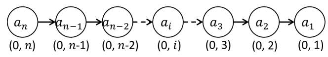
Figure 1: The chain with associated intervals.

The above example shows that a customised storage scheme saves time and space during construction, and also efficiently supports query answering. However, in typical application scenarios, a Datalog program $\Pi$ usually contains multiple different rules, and different optimisations may apply. How to combine different storage schemes and enable their integration with standard reasoning algorithms remains a challenge. In our example, $\Pi$ may include other rules that also derive $R$ facts, and it is essential that the interaction between such rules and the transitive rule is properly handled. Moreover, to enable seminaïve evaluation, the optimised storage schemes should provide efficient access to different portions of the derived facts (i.e., ‘$I$’, ‘$\Delta$’, ‘$I\cup\Delta$’), which will involve nontrivial adaptation of existing approaches.

We address the above issues by first introducing a general framework which involves the specification of several interfaces that each storage scheme must implement. We then present details of two useful storage schemes, focusing on the implementation of the relevant interfaces.

Multi-Scheme Framework

Algorithm 2 Multi-SchemeReasoning($\Pi,E,E^{+}$)

1:Result: update $I$ from $\Pi^{\infty}[E]$ to $\Pi^{\infty}[E\cup E^{+}]$

2:schedule$(E^{+}\backslash E)$ $\triangleright$ populate $\Delta_{n}^{T}$ and $C_{T}$

3:loop

4:     $\Delta=$ derive() $\triangleright$ apply $\Pi_{T}$ and update $\Delta^{T}$

5:     if $\Delta=\emptyset$ then break      

6:     for every scheme $T$ do

7:         schedule($\Delta^{T}$) $\triangleright$ populate $\Delta_{n}^{T}$ and $C_{T}$

8:         $T$.merge() $\triangleright$ merge $\Delta^{T}$ to $I^{T}$, empty $\Delta^{T}$      

Our framework incorporates multiple storage schemes that are responsible for managing disjoint sets of facts. In particular, each storage scheme $T$ deals with facts corresponding to predicates appearing in $P_{T}$, and it is associated with rules $\Pi_{T}\subseteq\Pi$ that use predicates in $P_{T}$ in the head. Additionally, to facilitate representation, we use another set of predicates $SP_{T}$ to denote the predicates used in the body of rules in $\Pi_{T}$. Moreover, an internal data structure $D_{T}$ maintains facts in $T$ and a fact cache $C_{T}$ is used to temporarily store the input facts. Finally, we denote by $I^{T}$the facts in the domain ‘$I$’ managed by scheme $T$. Similarly, we denote by $\Delta^{T}$the facts in the domain ‘$\Delta$’ managed by scheme $T$. To work with different schemes correctly during the materialisation, each scheme should implement the following functions.

1. The schedule function identifies facts with predicate in $SP_{T}$, and stores them in $C_{T}$ so that these facts can be used by $\Pi_{T}$ to derive new facts. An input fact $t$ with the predicate in $P_{T}$ is added to a set $\Delta_{n}^{T}$ if $t\notin$ $\Delta^{T}$$\cup$ $I^{T}$. This function does not change $\Delta^{T}$or $I^{T}$for a scheme $T$; it only schedules facts for later computation of $\Delta^{T}$.

2. The derive function applies rules in $\Pi_{T}$ and incorporates new facts in the data structure. The function does not modify $I^{T}$ but updates $\Delta^{T}$ as follows.

   $$\Delta^{T} =\Delta_{n}^{T}\cup\Pi_{T}^{+}[I,C_{T}].$$ (3)

3. The merge function updates $I^{T}$to $I^{T}$$\cup$$\Delta^{T}$, empties $\Delta^{T}$.

The global schedule function invokes schedule functions of every scheme. The global derive function calls derive functions of every scheme, and returns all facts in domain ‘$\Delta$’. The reasoning algorithm incorporating multiple storage schemes is shown in algorithm 2. It exploits principles similar to the modular materialisation approach. The main difference is that our approach additionally manages the (possibly compact) representation of derivations for different parts of the program. In line 2, relevant facts are identified for each scheme. In line 4, rules in $\Pi_{T}$ are applied in each scheme, and the data structure $D_{T}$ is updated to incorporate facts in $\Delta_{n}^{T}$ and the newly derived consequences into $\Delta^{T}$. Then in line 7, $\Delta^{T}$ are scheduled for insertion into different schemes before being merged to $I^{T}$ in line 8. In contrast to the modular materialisation approach in which a module $T$ computes only $\Pi_{T}^{+}[I,\Delta]$, our approach additionally considers $\Delta_{n}^{T}$ as part of $\Delta^{T}$ in (3). This is to make our framework general enough to capture storage schemes that do not explicitly store facts and thus cannot easily distinguish between their input and consequences. As we shall see, our storage scheme for transitive relations benefits from this generalisation. The following theorem states that algorithm 2 is correct, and its proof is provided in the appendix.

Theorem 1

A fact can be derived and represented in relevant schemes by the multi-scheme algorithm if and only if it can be derived by the modular seminaïve algorithm.

Plain Table: In practice, predicates and rules that are not handled by customised storage schemes are managed by a plain table. The plain table, as the name suggests, stores facts faithfully without any optimisations. The internal data structure $D_{T}$ can be implemented, for example, as a fact list $L_{T}$, in which each fact is assigned a label, either ‘$\Delta$’ or ‘$I$’. Then $I^{T}$ and $\Delta^{T}$ are defined intuitively as facts with the corresponding label. The derive function adds facts in $\Delta_{n}^{T}$ to $L_{T}$ and marks them as ‘$\Delta$’. Also, derivations in $\Pi_{T}[I,C_{T}]$ are added to the list $L_{T}$ with the label ‘$\Delta$’ if they are not in the list. The merge function is realised by simply changing the label of facts. It is easy to verify that the plain table satisfies the requirement of a scheme.

TC Storage Scheme

This section presents a specialised transitive closure (TC) scheme capable of efficiently handling transitively closed relations. The implementation of the scheme’s functions is based on nontrivial adaptations of the interval-based approach by Agrawal, Borgida, and Jagadish (1989), which treats TC computation as solving reachability problems over a graph. More specifically, each node is assigned an interval that compactly represents the (indexes of) nodes it can reach. The original approach does not accommodate access to facts in various domains (i.e., ‘$I$’, ‘$\Delta$’, ‘$I\cup\Delta$’). Furthermore, their discussion of incremental updates does not encompass all cases. Our extension of the technique enables multi-scheme reasoning by supporting access to different domains and providing more comprehensive incremental update procedures.

Interval-based Approach: For a set of input facts represented by a graph $G$, the approach computes a tree cover of the graph. Each node of the graph is numbered based on the post-order traversal of the tree. Then, an initial interval is assigned to each node with its post-order index being the upper bound, and the smallest lower-end number among its descendants’ intervals being the lower bound. For leaves, the lower bound is its index. The initial intervals capture the reachability of the tree. Then, for every edge $(i,j)\in G$ that is not in the tree cover, the interval of $j$ is added to $i$ and all its ancestors. The final intervals capture all reachable pairs in $G$. Just as expression (2), for each node in $G$, facts in the closure with this node as the first constant can be accessed using the computed intervals and indexes.

Settings: For the remainder of this section, we assume there is a rule $r\in\Pi$ that axiomatises a relation $R$ as transitive; the predicate set $P_{T}$ contains $R$ (and so $r$ is in $\Pi_{T}$). Additionally, for the ease of presentation, we assume that $\Pi_{T}$ contains only $r$. In reality, $T$ could also handle other rules that derive $R$ facts: these rules are applied using a standard algorithm, and the output is stored and processed by $T$.

Incremental Update and Fact Access

We now discuss how customised storage schemes deal with incremental insertion, which is crucial for integrating with standard reasoning algorithms. Notice that the original approach by Agrawal, Borgida, and Jagadish (1989) already considered incremental insertion. However, their discussion does not cover all possible insertion cases and the distinction between facts in domains ‘$I$’ and ‘$\Delta$’ is not allowed, which is a key requirement in the Datalog reasoning setting.

Naive Approach: One seemingly straightforward solution to supporting the distinction between ‘$I$’ and ‘$\Delta$’ facts is to have two sets of intervals for each node $s$: $s.In$ and $s.D$ contain indexes that $s$ can reach before the insertion and that $s$ can additionally reach after the insertion, respectively. Let $I_{s}$ and $\Delta_{s}$ be the facts with $s$ as the first constant in ‘$I$’ and ‘$\Delta$’, respectively, then $\Delta^{T}$ and $I^{T}$ can be defined as follows:

$$I_{s} =\{R(s,x)\ |\ x.id\in s.In\},$$ (4)

$$\Delta_{s} =\{R(s,x)\ |\ x.id\in s.D\},$$ (5)

$$\Delta^{T} =\{\Delta_{s}\ |\ s\in G\},\text{$I^{T}$}=\{I_{s}\ |\ s\in G\}.$$ (6)

The merge function merges ‘$\Delta$’ to ‘$I$’ by simply adding $s.D$ to $s.In$ and emptying $s.D$ afterwards.

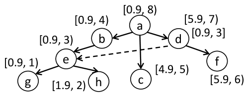
Figure 2: One example interval tree. The dashed edge is an edge in the graph but not covered by the tree cover.

The Problem of Fresh Nodes: We use an example to show why the naive approach is insufficient in the presence of fresh nodes. Assume that we insert a fresh node $k$ and a new edge $(d,k)$ to the graph shown in Figure 2. The tree cover is supposed to cover all the nodes, so $(d,k)$ is added to the tree cover. Instead of re-assigning the post-order index based on the updated tree, we assign a new post-order number to $k$ by finding a number $i$ so that $i$ is included in the initial interval of $d$ and $i$ is not occupied by any existing nodes, as suggested by Agrawal, Borgida, and Jagadish (1989). After insertion, the intervals would still be valid if we did not intend to distinguish between “$I$” and “$\Delta$”. However, following the naive approach we have $k.id\in d.In$, and so $R(d,k)\in$ $I^{T}$, which is not as expected since $(d,k)$ is newly inserted.

We propose to have another set of intervals $s.N$ to memorise the reachable nodes that are freshly introduced, where $s.N\subseteq s.In\cup s.D$. So new nodes in $s.In$ can be identified and skipped when accessing $I^{T}$, and they can be returned in addition to nodes in $s.D$ when accessing $\Delta^{T}$. Formally:

$$I_{s} =\{R(s,x)\ |\ x.id\in s.In\backslash s.N\},$$ (7)

$$\Delta_{s} =\{R(s,x)\ |\ x.id\in s.D\cup s.N\},$$ (8)

in which we treat a set of intervals as the set of numbers it covers, and set operators such as intersection ($\cap$), union ($\cup$ or +) and minus ($\backslash$) naturally apply. The $\Delta^{T}$ and $I^{T}$ are defined in the same way as in expression (6). Notice that to allow for the insertion of edges involving fresh nodes, when creating the initial intervals, we should allow for gaps. This could be achieved, for example, through special treatment for the leaf nodes: the lower end of the interval is set to be the current node index minus a small margin (e.g., 0.1), as illustrated in Figure 2.

Graph with Cycles: While the previous discussion assumes the graph constructed from the input facts is acyclic in the initial construction of the data structure, the same technique can also be applied to a cyclic graph by collapsing each strongly connected component to a node. Let $G_{0}$ and $G$ be the graph before and after condensation, respectively, and let $M$ be a mapping that maps each SCC in $G$ to its corresponding nodes in $G_{0}$. Then, the indexes and intervals are assigned to SCCs of the graph after condensation in the same way as described above. For each $s\in G$, sets $I_{s}$ and $\Delta_{s}$ denoting the corresponding sets of facts from $G_{0}$ in domains ‘$I$’ and ‘$\Delta$’ , respectively, can be obtained as follows:

$$I_{s} =\{M(s){\mkern-2.0mu\times\mkern-2.0mu}M(x)|\ x.id\in s.In\backslash s.N\},$$ (9)

$$\Delta_{s} =\{M(s){\mkern-2.0mu\times\mkern-2.0mu}M(x)|\ x.id\in s.D\cup s.N\},$$ (10)

in which $M(s){\mkern-2.0mu\times\mkern-2.0mu}M(x)$ computes the cross-product between the two sets of constants $M(s)$ and $M(x)$; for brevity, the predicate $R$ is omitted. Finally, $\Delta^{T}$ and $I^{T}$ are the same as in expression (6).

The Merging of Components: A tricky case not discussed in the original approach is that fact additions could possibly lead to the merging of existing SCCs. For example, if an edge $(h,d)$ is introduced, then the SCC $e,h$ and $d$ need to be merged as a new SCC. The graph can be updated by choosing $e$ as a representative node and deleting nodes $h$ and $d$. The children of $h$ and $d$ will be inherited to $e$. However, it is not straightforward how to maintain the intervals and access facts in $I^{T}$ and $\Delta^{T}$ correctly. For SCCs that are not merged during fact additions, expressions (9) and (10) are still valid to use. We distinguish between different SCCs by their status $St$: the status of an SCC that is not merged is stable; the status of an SCC that is merged and selected to be representative is new; the status of an SCC that is merged to a representative SCC is dropped. For a new SCC $e$, we use $e.D$ to store the interval that includes the indexes of nodes that $e$ can reach after merging regardless of the domain, and $e.N$ includes newly introduced nodes in $e.D$, so $e.N\subseteq e.D$. Intuitively, the node $e$ after merging is able to reach all the nodes in this newly merged component, as well as their descendants, so $e.D=\bigcup_{s\in F(e)}\{s.In\cup s.D\cup[s.id]\}$, in which $F$ is the map from the SCCs in the new graph to the original ones, and $[s.id]$ is a singleton interval that only includes $s.id$. In this example, $F(e)=\{e,h,d\}$. Similarly, $e.N$ also takes the union of $s.N$ for $s\in F(e)$, i.e., $e.N=\bigcup_{s\in F(e)}\{s.N\}$. Let $L$ be a list of SCCs ordered by their post-order indexes. Intervals and other associated information of SCCs are stored in $L$. Instead of deleting dropped SCCs in $L$ right away, we keep the original $In$, $id$, and $M$ map of each node $s\in F(e)$ in $L$. In this way, $\Delta_{s}$ and $I_{s}$ can be recomputed as follows:

$$I_{s} =\{M(s){\mkern-2.0mu\times\mkern-2.0mu}M(x)|\ x.id\in s.In\backslash e.N\},$$ (11)

$$\Delta_{s} =\{M(s){\mkern-2.0mu\times\mkern-2.0mu}M(x)|\ x.id\in(e.D\backslash s.In)\text{+}(e.N\cap s.In)\},$$

in which $e$ is the representative node of merged components so that $s\in F(e)$. In the merge function of the TC storage scheme, dropped SCCs in $L$ are deleted, $F$ map is emptied, and $M$ map of new nodes is updated to the union of members of original SCCs. Moreover, the status of new nodes is changed to stable, and $D$ interval is merged to $In$, $N$ and $D$ intervals are emptied.

The designs discussed above make the TC storage scheme suitable to use in the multi-scheme reasoning algorithm. For brevity and ease of understanding we have only highlighted the key aspects of the approach. Readers interested in an exhaustive (and lengthy) presentation of the algorithmic details of the storage scheme are invited to consult the appendix.

Union Storage Scheme

The union storage scheme is motivated by rules with the form: $A(x,y)\rightarrow U(x,y),B(x,y)\rightarrow U(x,y).$ The facts with predicate $U$ can be derived by ‘copying’ the instantiations from $A$ and $B$ facts. Therefore, instead of deriving and storing all the consequences of the above rules, we can have a ‘virtual’ storage for the facts with predicate $U$. Assume we have a union table $T$ for $U$; $\Pi_{T}$ contains all the rules $r\in\Pi$ such that $r$ is of the form $p(x,y)\rightarrow U(x,y)$; for brevity we again assume that there is no other rule in $\Pi$ that derives $U$ facts; the set $SP_{T}$ contains predicates used in the body of rules in $\Pi_{T}$. For the above example, $SP_{T}=\{A,B\}$. The internal data structure in the union table is a fact list $L_{T}$: if a fact with $U$ is explicitly defined and cannot recover from $\Pi_{T}$, then this fact will be stored in $L_{T}$.

For a predicate $p$, $I_{p}$ and $\Delta_{p}$ denote the facts with predicate $p$ in corresponding domains. The function responsible for computing $I^{T}$, as well as the implementation of the interfaces required by our framework, is described in algorithm 3. The $U$ facts are the ‘union’ of facts with predicates in $P_{T}$ and $SP_{T}$, so the $I^{T}$ set first collects explicit facts in $L_{T}$ with label ‘$I$’. Then, the remaining facts are translated from the supporting facts belonging to the same domain. Note that the function call $U(\vec{x}).sub(t)$ obtains the instantiation from $t$ and uses it to instantiate $U(\vec{x})$. In the schedule function, only facts with the predicate in $P_{T}$ or $SP_{T}$ are relevant for processing. If the fact passes the relevance check but cannot be recovered from $I_{p}$ (line 10), then the corresponding $U$ fact must be new and should be included in domain ‘$\Delta$’ in the derivation stage. To prepare for such derivation, there are two distinct cases: if $t$ has predicate $U$, then $t$ is added to the list $L_{T}$ with label ‘$\Delta_{n}$’ (line 11); if $t$ has predicate appearing in $SP_{T}$, then a $U$ fact instantiated by $t$ is added to $C_{T}$ for later use (line 12). The derive function changes facts with the label ‘$\Delta_{n}$’ to ‘$\Delta$’. The set $\Delta^{T}$ includes the ‘$\Delta$’ facts in $L_{T}$, and translated facts in $C_{T}$. The use of $C_{T}$ in derive and schedule is only for the sake of better presentation. In reality, the fact translation is done on the fly and thus does not incur significant memory overhead. The merge function is realised by changing facts that are explicitly stored in $L_{T}$ with the label ‘$\Delta$’ to ‘$I$’. It can be verified that the above implementation satisfies the definition of a scheme, and the proof is provided in the appendix.

Algorithm 3 Functions of Union Table

1:$T$: a union table;  $t$: a fact;  $L_{T}$: the fact list in $T$.

2:$D_{T}:$ implemented as $L_{T}$.  Assume $P_{T}=\{U\}$.

3:$\Pi_{T}=\{r\ |\ r=p(\vec{x})\rightarrow U(\vec{x})\in\Pi\}$.

4:procedure compute $I^{T}$

5:     $I^{T}$$:=\{t\in L_{T}\ |\ \text{the label of }t=$ ‘$I$’$\}$

6:     for $p\in SP_{T}$, for $t\in I_{p}$ do

7:         $I^{T}$$:=\text{$I^{T}$}\cup\{U(\vec{x}).sub(t)\}$      

8:procedure $T.$schedule($t$)

9:     if $t.p\notin P_{T}\cup SP_{T}$ then return      

10:     if $p(\vec{x}).sub(t)$ $\notin I_{p}$ for any $p\in SP_{T}\cup P_{T}$ then

11:         if $t.p\in P_{T}$ then add $t$ to $L_{T}$ as ‘$\Delta_{n}$’          

12:         if $t.p\in SP_{T}$ then $C_{T}:=C_{T}\cup\{U(\vec{x}).sub(t)\}$               

13:procedure $T.$derive()

14:     mark facts in $L_{T}$ with ‘$\Delta_{n}$’ as ‘$\Delta$’

15:     $\Delta^{T}$$:=\{t\in L_{T}\ |\ \text{the label of }t=$ ‘$\Delta$’$\}$

16:     $\Delta^{T}$$:=\Delta^{T}\cup C_{T}$,  $C_{T}=\emptyset$

Evaluations

	159,561 $\triangleright$ 29,086,642			29,086,642 $\triangleright$ 29,807,285			29,807,285 $\triangleright$ 30,717,549			30,717,549 $\triangleright$ 53,928,267
	time	peak	static	time	peak	static	time	peak	static	time	peak	static
Standrad	2,845.08	1,480.58	1,251.77	96.02	1,483.22	1,275.57	92.07	1,483.22	1,305.44	6,352.03	2,750.76	2,340.10
TCModule	28.24	1,554.44	1,320.64	15.50	1,564.41	1,358.62	2.78	1,564.41	1,374.29	39.42	2,845.42	2,414.81
TCScheme	8.44	249.64	248.01	0.84	249.74	248.01	0.91	249.77	248.01	6.06	284.93	278.26
	1,426,588 $\triangleright$ 1,949,306,188			1,949,306,188 $\triangleright$ 1,950,379,470			1,950,379,470 $\triangleright$ 1,951,309,711			1,951,309,711 $\triangleright$ 1,953,752,969
	time	peak	static	time	peak	static	time	peak	static	time	peak	static
Standrad	$>$38h	-	-	-	-	-	-	-	-	-	-	-
TCModule	3295.25	97,940.15	82,348.18	138.40	97,940.15	82,101.52	30.04	97,940.15	82,132.15	1519.99	98,406.95	82,548.45
TCScheme	443.80	2,447.91	2,304.00	2.22	2,447.91	2,304.84	2.96	2,447.91	2,304.85	14.84	2,447.91	2,304.87

Table 1: Performance Evaluation of TC Scheme Algorithms on DBpedia’s broader relation. The bold text indicates changes in the fact count before and after materialisation. The time is in second, peak and static stand for the peak memory usage during the reasoning and the static memory used by the data structure, respectively. Both of the memory are reported in MB.

	DB25% (23.0M $\triangleright$ 32.7M); Union: 4.2M; TC: 677.8k $\triangleright$ 4.2M					DB50% (46.0M $\triangleright$ 608.7M); Union: 280.2M; TC: 1.4M $\triangleright$ 280.2M					DAG (100k $\triangleright$ 22.9M)
	time	peak	static	$NT$	other $T$	time	peak	static	$NT$	other $T$	time	peak	static	$NT$	other $T$
Standard	33.42	2.7	2.2	2.2	-	12,879.90	30.8	25.4	25.4	-	3,973.21	1.1	0.9	0.9	-
TCModule	33.88	3.2	2.7	2.2	-	984.86	31.8	26.4	25.4	-	36.04	1.2	1.0	0.9	-
MultiScheme	31.39	3.6	3.1	1.9	1.2	479.35	8.7	7.7	3.1	4.6	26.45	0.9	0.9	0.01	0.89
	DB75% (69.0M $\triangleright$ 8.6B); Union: 4.3B; TC: 2.0M $\triangleright$ 4.3B					DBAll (92.0M $\triangleright$ 34.9B); Union: 17.4B; TC: 2.7M $\triangleright$ 17.4B					Relations (845.8k $\triangleright$ 212.2M); Union: 191.0M; TC: 390.3k $\triangleright$ 14.1M
	time	peak	static	$NT$	other $T$	time	peak	static	$NT$	other $T$	time	peak	static	$NT$	other $T$
Standard	>86h	-	-	$\approx$515	-	-	-	-	$\approx$2094.9	-	14,277.00	11.0	9.3	9.2	-
TCModule	>86h	-	-	-	-	-	-	-	-	-	2,046.36	11.1	9.4	9.2	-
MultiScheme	5,973.34	16.3	14.9	4.0	10.9	23,092.37	17.3	15.1	5.6	9.5	6,905.72	4.9	4.1	3.6	0.5

Table 2: Performance Evaluation of Multi-Scheme Reasoning Algorithm. Time is in seconds. The other four metrics are in GB, in which $NT$ and ‘other $T$’ mean the memory used by the normal plain table and other schemes, respectively.

Benchmarks: We tested our algorithms on DAG-R (Hu, Motik, and Horrocks 2022), DBpedia (Lehmann et al. 2015), and Relations (Smith et al. 2007). DAG-R is a synthetic benchmark, containing a randomly generated directed acyclic graph with 100k edges and 10k nodes and a Datalog program in which the connected property is transitive. DBpedia consists of structured information from Wikipedia. The SKOS vocabulary is used to represent various Wikipedia categories. We used a Datalog subset of the SKOS RDF schema as rules for DBpedia, in which several transitive and union rules are present. The Relations benchmark is obtained from the Relations Ontology (Smith et al. 2007) containing numerous biomedical ontologies. The converted Datalog program consists of 1307 rules in total, $33$ TC schemes and $130$ Union schemes are created according to the program. The original ontology does not have data associated, so we use the synthetic dataset created by Hu, Motik, and Horrocks (2022).

Compared Approaches: We considered three approaches for the evaluation of materialisation time and memory consumption. The standard approach applies the seminaïve algorithm for materialisation and uses just normal tables for storage. The Multi-Scheme is our proposed approach, using a plain table, TC and Union schemes. The TC Module approach proposed by Hu, Motik, and Horrocks (2022) applies an optimised application of TC rules, and a standard seminaïve algorithm for the remaining rules, but only a plain table is used for storage. The original modular approach also proposes optimisations for other types of rules, such as chain rules. For a fair comparison, we evaluate a version where only the optimisation for transitive closure rules is enabled.

Test Setups: All of our experiments are conducted on a Dell PowerEdge R730 server with 512GB RAM and 2 Intel Xeon E5-2640 2.60GHz processors, running Fedora 33, kernel version 5.10.8.

Performance of TC Scheme Algorithms: To comprehensively evaluate the performance of the proposed TC functions, we extracted two sets of broader facts from DBpedia and created a program with a transitive rule for broader. For each dataset, we inserted the facts in four rounds: the first insertion added all remaining facts (shown in the first column of Table 1), while the next three insertions each added 1,000 new facts as $E^{+}$ to test incremental maintenance (the last three columns). For the smaller dataset (the upper rows), the TC Module approach optimised the running time to a large extent compared to the standard approach, but not on memory consumption. In contrast, our TC scheme approach is around 100-1000x faster than the standard approach, but only uses about 1/8 $\sim$ 1/5 memory, in all the tasks. For the larger dataset (the lower rows), the standard approach failed to finish the initial insertion. Our TC scheme approach finished all the tasks and only used around 1/35 of the memory used by the TC Module. Our TC scheme can also maintain the data structure quickly under addition (around 7-100x faster than the TC Module), which is beneficial for the recursive and incremental reasoning scenario.

Performance of Multi-Scheme Reasoning Algorithms: We tested the performance of our proposed multi-scheme reasoning algorithm on the benchmarks mentioned above. A scalability evaluation was conducted by randomly choosing subsets from DBpedia. As shown in Table 2, our multi-scheme approach used slightly more time and memory than the standard approach when the dataset is small (DB25%), since the fraction between the output TC facts and the input TC facts is small, benefits of using the compressed data structure does not show. However, for 50% subset of DBpedia, our approach is 27x faster than the standard approach and only uses 1/3 memory. In the reasoning process, TC and union schemes naturally consume more time to traverse the contained facts than the plain table, which will lead to longer rule application time for the multi-scheme approach. But this approach is still faster than applying TC and union rules faithfully as done in the standard approach. The standard and TC Module approach cannot finish the materialisation for 75% and the whole DBpedia; while our approach completes the materialisation only using around $15$ GB. In contrast, storing the materialisation of 75% and full DBpedia is estimated to take $515$ GB and $2094.9$ GB respectively.

For DAG-R, using TC schemes speeds up runtime but does not reduce memory usage by much, due to the size of the TC closure. For Relations, the TC rule optimisation in the TC Module significantly decreases materialisation time, but not memory usage. In contrast, our approach finishes materialisation using less than half the memory of the standard and TC Module approaches. However, the presence of union predicates in some rule bodies requires traversing facts represented by union schemes, increasing running time, though it is still faster than the standard approach.

TC Query	$Q_{0}$ (140M)	$Q_{1}$ (140M)	$Q_{3}$ (428)	$Q_{7}$ (752k)	$Q_{8}$ (1M)
Standard	8.38	27.70	0.03	0.10	0.13
MultiScheme	22.43	20.62	0.03	0.24	0.35
Union Query	$Q_{0}$ (280M)	$Q_{2}$ (753k)	$Q_{3}$ (1M)	$Q_{4}$ (337)	$Q_{8}$ (1M)
Standard	25.50	0.28	0.42	0.03	0.15
MultiScheme	338.90	0.61	0.89	0.03	2.93

Table 3: The Query Answering Time in seconds. The cardinality of each query is provided in the brackets.

Performance of Query Answering: One potential disadvantage of the multi-scheme framework is increased query retrieval time. To fully characterise this trade-off, we evaluated query performance using $11$ queries with transitive predicates and $11$ queries with union predicates. Instead of using queries with complex graph patterns, we employ queries with 1 or 2 atoms using the TC or union predicate to capture the performance of specialised storage schemes. Query execution times were conducted in 50% subset of DBpedia and compared against the standard approach. Due to page limits, Table 3 presents results for 5 queries with transitive predicates in the upper rows and 5 queries with union predicates at the bottom; the complete table and all queries are provided in the appendix. The evaluation results suggest that for queries with small cardinality (usually less than 1 million), the running time is not significantly different. For queries with the transitive predicate, our approach consumes less than 3 times of the time used by the standard approach. For queries with union predicates, it is around 2-20 times, since retrieval from union schemes includes querying other schemes to remove the duplicate and verify the status of related facts.

Discussion and Perspectives

In this paper, we proposed a framework that can accommodate different storage and reasoning optimisations. Our approach offers a flexible and extensible alternative that supports Datalog reasoning applications in scenarios where storage resource is limited and materialisation fails. Future work will involve supporting deletion in the multi-scheme framework and introducing deletion functions for specialised tables. For example, maintaining the data structure in the TC scheme will require handling the collapse of an SCC caused by deletion.

See pages 1,2,3,4,5,6,7,8,9,10,11 of appendix.pdf

References

- Abiteboul, Hull, and Vianu (1995) Abiteboul, S.; Hull, R.; and Vianu, V. 1995. Foundations of databases, volume 8. Addison-Wesley Reading.
- Agrawal, Borgida, and Jagadish (1989) Agrawal, R.; Borgida, A.; and Jagadish, H. V. 1989. Efficient management of transitive relationships in large data and knowledge bases. ACM SIGMOD Record, 18(2): 253–262.
- Aref et al. (2015) Aref, M.; ten Cate, B.; Green, T. J.; Kimelfeld, B.; Olteanu, D.; Pasalic, E.; Veldhuizen, T. L.; and Washburn, G. 2015. Design and implementation of the LogicBlox system. In Proceedings of the 2015 ACM SIGMOD International Conference on Management of Data, 1371–1382.
- Bellomarini, Gottlob, and Sallinger (2018) Bellomarini, L.; Gottlob, G.; and Sallinger, E. 2018. The Vadalog system: Datalog-based reasoning for knowledge graphs. arXiv preprint arXiv:1807.08709.
- Carral et al. (2019) Carral, D.; Dragoste, I.; González, L.; Jacobs, C.; Krötzsch, M.; and Urbani, J. 2019. Vlog: A rule engine for knowledge graphs. In International Semantic Web Conference, 19–35. Springer.
- Gupta, Mumick, and Subrahmanian (1993) Gupta, A.; Mumick, I. S.; and Subrahmanian, V. S. 1993. Maintaining views incrementally. ACM SIGMOD Record, 22(2): 157–166.
- Horrocks et al. (2004) Horrocks, I.; Patel-Schneider, P. F.; Boley, H.; Tabet, S.; Grosof, B.; Dean, M.; et al. 2004. SWRL: A semantic web rule language combining OWL and RuleML. W3C Member submission, 21(79): 1–31.
- Hu, Motik, and Horrocks (2022) Hu, P.; Motik, B.; and Horrocks, I. 2022. Modular materialisation of datalog programs. Artificial Intelligence, 308: 103726.
- Lehmann et al. (2015) Lehmann, J.; Isele, R.; Jakob, M.; Jentzsch, A.; Kontokostas, D.; Mendes, P. N.; Hellmann, S.; Morsey, M.; van Kleef, P.; Auer, S.; and Bizer, C. 2015. DBpedia - A large-scale, multilingual knowledge base extracted from Wikipedia. Semantic Web, 6(2): 167–195.
- Motik et al. (2015) Motik, B.; Nenov, Y.; Piro, R.; and Horrocks, I. 2015. Handling owl: sameAs via rewriting. In Proceedings of the AAAI Conference on Artificial Intelligence, volume 29.
- Motik et al. (2019) Motik, B.; Nenov, Y.; Piro, R.; and Horrocks, I. 2019. Maintenance of datalog materialisations revisited. Artificial Intelligence, 269: 76–136.
- Motik et al. (2009) Motik, B.; Patel-Schneider, P. F.; Parsia, B.; Bock, C.; Fokoue, A.; Haase, P.; Hoekstra, R.; Horrocks, I.; Ruttenberg, A.; Sattler, U.; et al. 2009. OWL 2 web ontology language: Structural specification and functional-style syntax. W3C recommendation, 27(65): 159.
- Nenov et al. (2015) Nenov, Y.; Piro, R.; Motik, B.; Horrocks, I.; Wu, Z.; and Banerjee, J. 2015. RDFox: A highly-scalable RDF store. In International Semantic Web Conference, 3–20. Springer.
- Smith et al. (2007) Smith, B.; Ashburner, M.; Rosse, C.; Bard, J.; Bug, W.; Ceusters, W.; Goldberg, L. J.; Eilbeck, K.; Ireland, A.; Mungall, C. J.; et al. 2007. The OBO Foundry: coordinated evolution of ontologies to support biomedical data integration. Nature biotechnology, 25(11): 1251–1255.
- Staudt and Jarke (1995) Staudt, M.; and Jarke, M. 1995. Incremental maintenance of externally materialized views. Citeseer.
- Subercaze et al. (2016) Subercaze, J.; Gravier, C.; Chevalier, J.; and Laforest, F. 2016. Inferray: fast in-memory RDF inference. In VLDB, volume 9.
- Wu et al. (2008) Wu, Z.; Eadon, G.; Das, S.; Chong, E. I.; Kolovski, V.; Annamalai, M.; and Srinivasan, J. 2008. Implementing an inference engine for RDFS/OWL constructs and user-defined rules in Oracle. In 2008 IEEE 24th International Conference on Data Engineering, 1239–1248. IEEE.