Special Function solutions of Painlevé-IV and the Quartic Model

Abstract.

The fourth Painlevé equation, known as Painlevé-IV, is a family of differential equations depending on two complex parameters and is given by

$$\mathinner{\dfrac{\operatorname{d\!}{{}^{2}}u}{\operatorname{d\!}{x^{2}}}}=\dfrac{1}{2u}\left(\mathinner{\dfrac{\operatorname{d\!}{}u}{\operatorname{d\!}{x}}}\right)^{2}+\dfrac{3}{2}u^{3}+4xu^{2}+2(x^{2}-\alpha)u+\dfrac{\beta}{u},\quad\alpha,\beta\in{\mathbb{C}}.$$

While generic solutions of Painlevé equations are known to be transcendental, five of the six equations admit solutions written in terms of classical special functions. In this work, we analyze a particular family of such solutions of Painlevé-IV given in terms of Parabolic Cylinder functions. We do so by establishing explicit formulas connecting these solutions and recurrence coefficients of polynomials orthogonal with respect to the measure ${\mathrm{e}}^{-V(z;t)}{\mathrm{d}}z$ were $V(z;t)=z^{4}/4+tz^{2}/2$. This particular family of polynomials appears in the study of the Quartic Random Matrix Model.

1. Introduction

This work centers around the interactions of three mathematical objects that have been the subject of intense study over the last few decades:

• solutions of Painlevé-IV,

• the Quartic One-Matrix Model, and

• Semi-classical orthogonal polynomials.

Each has given rise to a beautiful theory and a large body of work; we do not dare to attempt an exhaustive exposition of their literature. Instead, we settle for describing the bare minimum necessary for the reader to appreciate the connections between them.

1.1. Painlevé-IV

By now, the Painlevé equations are fundamental equations in integrable systems and mathematical physics. While generic solutions of Painlevé equations are highly transcendental, all but Painlevé-I possess special solutions written in terms of elementary and/or classical special functions (Airy functions, Bessel functions, parabolic cylinder functions, etc.). We will focus our attention on the fourth Painlevé equation, given by

($$\textnormal{P}_{IV} \mathinner{\dfrac{\operatorname{d\!}{{}^{2}}u}{\operatorname{d\!}{x^{2}}}}=\dfrac{1}{2u}\left(\mathinner{\dfrac{\operatorname{d\!}{}u}{\operatorname{d\!}{x}}}\right)^{2}+\dfrac{3}{2}u^{3}+4xu^{2}+2(x^{2}-\alpha)u+\dfrac{\beta}{u},\quad\alpha,\beta\in{\mathbb{C}}.$$)

Painlevé-IV possesses both rational solutions and solutions written in terms parabolic cylinder functions, see e.g. [BCH, GLS, MR0896355, MR0217352, O]. Rational solutions of ($\textnormal{P}_{IV}$) appear in various applications (see [BCH, BM] and references therein), and their large-degree asymptotics were recently obtained in [BM]. There, a different set of parameters than the ones in ($\textnormal{P}_{IV}$) is used; they are given by

(1.1) $$\alpha=2\Theta_{\infty}-1,\quad\beta=-8\Theta_{0}^{2}.$$

These parameters have natural interpretations in the recasting of ($\textnormal{P}_{IV}$) as the condition for isomonodromic deformation for an associated $2\times 2$ system of differential equations. While we will not use this fact, we will still adopt these parameters and denote solutions of ($\textnormal{P}_{IV}$), $u(x)$ with parameters given by (1.1) by the triple $(u(x),\Theta_{0},\Theta_{\infty})$. A different reformulation of ($\textnormal{P}_{IV}$) which we will make heavy use of is the following symmetric form of Painlevé-IV; see, e.g., [N]. We will follow the notation of [FW].

Theorem 1.1 ([Adler]).

Let $\{\alpha_{j}\}_{j=0}^{2}\in{\mathbb{C}}$ be arbitrary constants satisfying

(1.2) $$\alpha_{0}+\alpha_{1}+\alpha_{2}=1.$$

Consider the system

($$\textnormal{P}^{\textnormal{sym}}_{IV} \mathinner{\dfrac{\operatorname{d\!}{}f_{0}}{\operatorname{d\!}{x}}} =f_{0}(f_{1}-f_{2})+2\alpha_{0},$$)

$$\mathinner{\dfrac{\operatorname{d\!}{}f_{1}}{\operatorname{d\!}{x}}} =f_{1}(f_{2}-f_{0})+2\alpha_{1},$$

$$\mathinner{\dfrac{\operatorname{d\!}{}f_{2}}{\operatorname{d\!}{x}}} =f_{2}(f_{0}-f_{1})+2\alpha_{2},$$

along with the constraint

(1.3) $$f_{0}(x)+f_{1}(x)+f_{2}(x)=2x,$$

are equivalent to ($\textnormal{P}_{IV}$). That is, for $j=0,1,2$, $u(x)=-f_{j}(x)$ solves ($\textnormal{P}_{IV}$) with parameters

(1.4) $$\alpha=\alpha_{j-1}-\alpha_{j+1},\quad\beta=-2\alpha_{j}^{2}.$$

Furthermore, given a solution of ($\textnormal{P}_{IV}$), $(u(x),\Theta_{0},\Theta_{\infty})$, there exists a triple $(f_{0}(x),f_{1}(x),f_{2}(x))$ and parameters $(\alpha_{0},\alpha_{1},\alpha_{2})$ satisfying ($\textnormal{P}^{\textnormal{sym}}_{IV}$).

The symmetric form of ($\textnormal{P}^{\textnormal{sym}}_{IV}$) allows one to deduce various Bäcklund transformation; transformations that map a solution $(f_{0},f_{1},f_{2})$ to another triple which solves ($\textnormal{P}^{\textnormal{sym}}_{IV}$) with possibly modified parameters. Their connection with the already known Bäcklund transformations of ($\textnormal{P}_{IV}$) is discussed in Section 2.2. A key role will be played by three commuting transformations $T_{1},T_{2},T_{3}$, whose explicit description is given in Section 2.1, which act on the parameters $(\alpha_{0},\alpha_{1},\alpha_{2})$ is summarized in Table 1.

	$\alpha_{0}$	$\alpha_{1}$	$\alpha_{2}$
$T_{1}$	$\alpha_{0}-1$	$\alpha_{1}+1$	$\alpha_{2}$
$T_{2}$	$\alpha_{0}$	$\alpha_{1}-1$	$\alpha_{2}+1$
$T_{3}$	$\alpha_{0}+1$	$\alpha_{1}$	$\alpha_{2}-1$

Table 1. Action of $T_{i}$ on parameters $\alpha_{j}$.

Moving forward, we will use the notation $K_{n,m,k}(x)\mathrel{\mathop{\mathchar 58\relax}}=T_{3}^{k}T_{2}^{m}T_{1}^{n}(K_{0}(x))$ where $K$ is replaced by various relevant functions. Two such functions are the Jimbo-Miwa-Okamoto $\tau$- and $\sigma$-functions, which will play a key role in our results, are defined in Section 2.3.

It is well-known (see Section 2.5) that ($\textnormal{P}_{IV}$) (and therefore ($\textnormal{P}^{\textnormal{sym}}_{IV}$)) possesses solutions which can be written in terms of parabolic cylinder functions and complementary error function whenever either of following conditions hold:

$$\Theta_{0}\pm\Theta_{\infty}=0\quad\text{and}\quad\Theta_{0}\pm\Theta_{\infty}=1.$$

Starting with one such solution as a “seed” function and iterating Bäcklund transformations produces a families of special function solutions of Painlevé-IV. In this work, we will focus our attention on a particular family of parabolic cylinder solutions that appear in the Quartic One-Matrix Model which we now introduce.

1.2. Orthogonal Polynomials

Let $\{P_{n}(z;t,N)\}_{n=0}^{\infty}$ be the sequence of monic polynomials orthogonal satisfying

(1.5) $$\int_{{\mathbb{R}}}z^{k}P_{n}(z;t,N){\mathrm{e}}^{-NV(z;t)}{\mathrm{d}}z=0\quad\text{for}\quad k=0,1,...,n-1,$$

where

(1.6) $$V(z;t)\mathrel{\mathop{\mathchar 58\relax}}=\dfrac{z^{4}}{4}+\dfrac{tz^{2}}{2}.$$

Computing the polynomial $P_{n}$ amounts to solving an under-determined, homogeneous system of equations, and so it always exists, but may have degree smaller than $n$. Henceforth, we denote by $P_{n}$ the minimal degree monic polynomial satisfying (1.5), which is a unique object. When $t\in{\mathbb{R}}$ (we will always take $N\geq 0$) the measure of orthogonality in (1.5) is positive which implies $\text{deg}P_{n}=n$ for all $n\in{\mathbb{N}}$. When $t\in{\mathbb{C}}\setminus{\mathbb{R}}$, we can only assert that $\text{deg}P_{n}\leq n$. A key observation which we will make repeated use of is that $\text{deg}P_{n}(z;t,N)=n$ if and only if $H_{n-1}(t,N)\neq 0$, where

(1.7) $$H_{n-1}(t,N)=\det\left[\int_{\mathbb{R}}s^{i+j}{\mathrm{e}}^{-NV(s;t)}{\mathrm{d}}s\right]_{i,j=0}^{n-1}.$$

Orthogonal polynomials are known to satisfy a three-term recurrence relation; since the weight of orthogonality is even the relation takes the form

(1.8) $$zP_{n}(z;t,N)=P_{n+1}(z;t,N)+\gamma_{n}^{2}(t,N)P_{n-1}(z;t,N).$$

where

(1.9) $$\gamma_{n}^{2}(t,N)=\dfrac{h_{n}(t,N)}{h_{n-1}(t,N)}$$

and $h_{n}$ are the normalizing constants given by

(1.10) $$h_{n}(t,N)\mathrel{\mathop{\mathchar 58\relax}}=\int_{\mathbb{R}}P_{n}^{2}(z;t,N){\mathrm{e}}^{-NV(z;t)}{\mathrm{d}}z=\dfrac{H_{n}(t,N)}{H_{n-1}(t,N)}.$$

Since $H_{n}$ are entire functions of $t$, $\gamma_{n}^{2}(t,N)$ and $h_{n}(t,N)$ are meromorphic functions in $t$. To state our next main result, we need the following lemma, whose proof is given in Section 3.1.

Lemma 1.2.

Let $H_{n}(t,N)$ be as in (1.7). Set $H_{0}^{(e,o)}(t,N)\equiv 1$ and

(1.11) $$H^{(e)}_{n}(t,N) \mathrel{\mathop{\mathchar 58\relax}}=\det\left[\mathinner{\dfrac{\operatorname{d\!}{{}^{i+j}}}{\operatorname{d\!}{t^{i+j}}}}\left({\mathrm{e}}^{Nt^{2}/8}D_{-\frac{1}{2}}\left({N^{1/2}2^{-1/2}t}\right)\right)\right]_{i,j=0}^{n-1},$$

(1.12) $$H^{(o)}_{n}(t,N) \mathrel{\mathop{\mathchar 58\relax}}=\det\left[\mathinner{\dfrac{\operatorname{d\!}{{}^{i+j}}}{\operatorname{d\!}{t^{i+j}}}}\left({\mathrm{e}}^{Nt^{2}/8}D_{-\frac{3}{2}}\left({N^{1/2}2^{-1/2}t}\right)\right)\right]_{i,j=0}^{n-1},$$

where $D_{\nu}(\diamond)$ is the parabolic cylinder functions (cf. [DLMF]*Section 12). Then, we have the following identities

(1.13) $$H_{2n-1}(t,N) =\dfrac{\pi^{n}2^{2n(n-1)}}{N^{n(2n-1)}}H^{(e)}_{n}(t,N)H^{(o)}_{n}(t,N),$$

(1.14) $$H_{2n}(t,N) =\dfrac{\pi^{n+\frac{1}{2}}2^{2n^{2}+\frac{1}{4}}}{N^{2n^{2}+n+\frac{1}{4}}}H^{(e)}_{n+1}(t,N)H^{(o)}_{n}(t,N).$$

Our first result is that quantities related to the polynomials $P_{n}$ can be written, as functions of $t$, in terms of solutions to ($\textnormal{P}^{\textnormal{sym}}_{IV}$) and their $\tau$ and $\sigma$ functions in the following manner.

Theorem 1.3.

Let $\tau_{n,m,k},\sigma_{n,m,k},$ and $(f_{0})_{n,m,k},(f_{1})_{n,m,k},(f_{2})_{n,m,k}$ be the Bäcklund iterates of $\tau_{0,0,0},\sigma_{0,0,0}$ and the solution of ($\textnormal{P}^{\textnormal{sym}}_{IV}$) with parameters $(\alpha_{0},\alpha_{1},\alpha_{2})=(0,\frac{1}{2},\frac{1}{2})$ given by

$$(f_{0}(x),f_{1}(x),f_{2}(x))_{0,0,0}=\left(0,\frac{\varphi^{\prime}(x)}{\varphi(x)},2x-\frac{\varphi^{\prime}(x)}{\varphi(x)}\right),\quad\varphi(x)={\mathrm{e}}^{x^{2}/2}D_{-1/2}(\sqrt{2}x).$$

Then,

(1.15) $$\tau_{n-1,0,0}(x) ={\mathrm{e}}^{-(n-\frac{1}{2})x^{2}}H_{n}^{(e)}(2N^{-1/2}x,N)={\mathrm{e}}^{-(n-\frac{1}{2})x^{2}}H_{n}^{(e)}(2x,1),\vskip 6.0pt plus 2.0pt minus 2.0pt$$

(1.16) $$\tau_{n-1,-1,0}(x) ={\mathrm{e}}^{-(n+\frac{1}{2})x^{2}}H_{n}^{(o)}(2N^{-1/2}x,N)={\mathrm{e}}^{-(n+\frac{1}{2})x^{2}}H_{n}^{(o)}(2x,1),\vskip 6.0pt plus 2.0pt minus 2.0pt$$

(1.17) $$(f_{0})_{n,0,0}(x) =-N^{1/2}\gamma_{2n}^{2}(2N^{-1/2}x,N)=-\gamma_{2n}^{2}(2x,1),\vskip 6.0pt plus 2.0pt minus 2.0pt$$

(1.18) $$(f_{1})_{n,0,0}(x) =-N^{1/2}\gamma_{2n+1}^{2}(2N^{-1/2}x,N)=-\gamma_{2n+1}^{2}(2x,1),\vskip 6.0pt plus 2.0pt minus 2.0pt$$

(1.19) $$(f_{2})_{n,0,0}(x) =2x+N^{1/2}(\gamma_{2n}^{2}(2N^{-1/2}x,N)+\gamma_{2n+1}^{2}(2N^{-1/2}x,N)\vskip 6.0pt plus 2.0pt minus 2.0pt$$

$$=2x+\gamma_{2n}^{2}(2x,1)+\gamma_{2n+1}^{2}(2x,1).$$

Furthermore, writing

$$P_{n}(z;t,N)\mathrel{\mathop{\mathchar 58\relax}}=z^{n}+\sum_{k=1}^{\lfloor\frac{n}{2}\rfloor}\mathfrak{p}_{n,n-2k}(t,N)z^{n-2k},$$

we have

(1.20) $$\sigma_{n-1,0,0}(x) =N^{1/2}\mathfrak{p}_{2n,2n-2}(2N^{-1/2}x,N)-(2n-1)x\vskip 6.0pt plus 2.0pt minus 2.0pt$$

$$=\mathfrak{p}_{2n,2n-2}(2x,1)-(2n-1)x,\vskip 6.0pt plus 2.0pt minus 2.0pt$$

(1.21) $$\sigma_{n-1,-1,0}(x) =N^{1/2}\mathfrak{p}_{2n+1,2n-1}(2N^{-1/2}x,N)-(2n+1)x\vskip 6.0pt plus 2.0pt minus 2.0pt$$

$$=\mathfrak{p}_{2n+1,2n-1}(2x,1)-(2n+1)x.$$

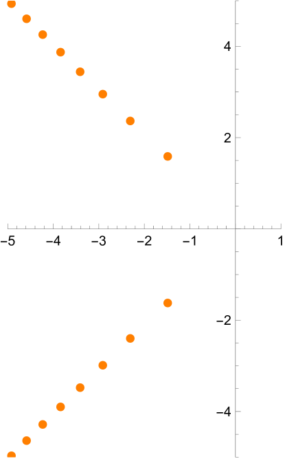
(a) $n=0$

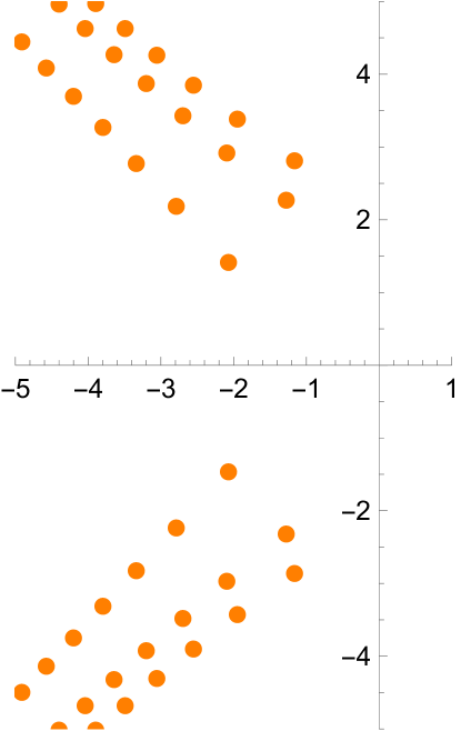
(b) $n=1$

Figure 1. Poles of $(f_{1})_{n,0,0}(x)$.

We prove Theorem 1.3 in Section 3.3. Figure 1 depicts the poles of $(f_{1})_{n,0,0}$, and while the figure depicts poles for small $n$, it appears that large swaths of the plane are free of poles. With Theorem 1.3 in hand, we can explain the lack of poles and study the large $n$ behavior of special function solutions of ($\textnormal{P}^{\textnormal{sym}}_{IV}$) by studying the coefficients $\gamma^{2}_{n}(t,N)$ and the zeros of $H_{n}(t,N)$. The particular choice of parameters in Theorem 1.3 is motivated by the Quartic One-Matrix Model, which we now introduce.

1.3. The Quartic Model

Let $\mathbf{M}$ be an $n\times n$ Hermitian matrix drawn with respect to the distribution

(1.22) $$\frac{1}{\tilde{\mathcal{Z}}_{nN}}{\mathrm{e}}^{-N\mathrm{Tr}\left(\mathcal{V}(\mathbf{M})\right)}{\mathrm{d}}\mathbf{M},$$

where $\mathcal{V}(x)\mathrel{\mathop{\mathchar 58\relax}}{\mathbb{R}}\to{\mathbb{R}}$ is a real-valued analytic function satisfying a particular growth condition as $x\to\infty$, and $\mathcal{V}(\mathbf{M})$ is understood using the spectral theorem. The set of such matrices is known in the literature as a unitarily invariant ensemble, see e.g. [BL]*Chapter 1. Unitarily invariant ensembles can be viewed as generalizations of the classical Gaussian Unitary Ensemble (GUE) and their connection with orthogonal polynomials on the real line is classical [Mehta].

The particular case where $\mathcal{V}(x)=\frac{1}{2}x^{2}+\frac{u}{4}x^{4}$ is often referred to as the Quartic One-Matrix Model. The eigenvalues of a matrix drawn from this ensemble have a joint probability density

$${\mathrm{d}}\mu_{nN}(z;u)=\dfrac{1}{\mathcal{Z}_{n}(u,N)}\prod^{n}_{1\leq k<j\leq n}(z_{k}-z_{j})^{2}\prod_{j=1}^{n}{\mathrm{e}}^{-N\left(\frac{1}{2}z_{j}^{2}+\frac{u}{4}z^{4}_{j}\right)}{\mathrm{d}}z_{1}\cdots{\mathrm{d}}z_{n}$$

and $\mathcal{Z}_{n}(u,N)$ is the eigenvalue partition function given by

(1.23) $$\mathcal{Z}_{n}(u,N)=\int_{{\mathbb{R}}}\cdots\int_{\mathbb{R}}\prod^{n}_{1\leq k<j\leq n}(z_{k}-z_{j})^{2}\prod_{j=1}^{n}{\mathrm{e}}^{-N\left(\frac{1}{2}z_{j}^{2}+\frac{u}{4}z^{4}_{j}\right)}{\mathrm{d}}z_{1}\cdots{\mathrm{d}}z_{n}.$$

The two partition functions in (1.22) and (1.23) are related by a classical formula

$$\dfrac{\mathcal{Z}_{n}(u,N)}{\tilde{\mathcal{Z}}_{n}(u,N)}=\dfrac{1}{\pi^{n(n-1)/2}}\prod_{j=1}^{n}j!.$$

The free energy of this ensemble is defined as

$$\mathcal{F}_{n}(u,N)\mathrel{\mathop{\mathchar 58\relax}}=\dfrac{1}{n^{2}}\log\dfrac{\tilde{\mathcal{Z}}_{n}(u,N)}{\tilde{\mathcal{Z}}_{n}(0,N)}=\dfrac{1}{n^{2}}\log\dfrac{{\mathcal{Z}}_{n}(u,N)}{{\mathcal{Z}}_{n}(0,N)}.$$

The quantity $\tilde{\mathcal{Z}}_{n}(0,N)$ is the partition function of the GUE and is given by (see, e.g., [BL]*Page 2)

$${\mathcal{Z}}_{n}(0,N)=\left(\dfrac{n}{N}\right)^{n^{2}}\dfrac{(2\pi)^{n/2}}{(2n)^{n^{2}/2}}\prod_{j=1}^{n}j!.$$

The Quartic Model was first investigated in [BIPZ, BIZ], where it was observed that when $n=N$, the free energy (1.25) admits an asymptotic expansion in inverse powers of $N^{-2}$ and that the coefficient of $N^{-2g}$, as functions of $u$, serve as generating functions for the number of four-valent graphs on a Riemann surface of genus $g$. This expansion came to be known as the topological expansion, and its existence was proven in [MR1953782] for matrix models with even polynomial potential.

While the model does not make sense when $u\in{\mathbb{C}}\setminus{\mathbb{R}}_{\geq 0}$, one can arrive at a quantity that can be readily analytically continued to the complex plane by starting with $u>0$ and letting

$$z_{j}=t^{1/2}\zeta_{j}\quad\text{and}\quad u=t^{-2},\ t>0.$$

Then, we arrive at

$${\mathcal{Z}}_{n}(u(t),N)=t^{n^{2}/2}\int_{{\mathbb{R}}}\cdots\int_{\mathbb{R}}\prod^{n}_{1\leq k<j\leq n}(\zeta_{k}-\zeta_{j})^{2}\prod_{j=1}^{n}{\mathrm{e}}^{-N\left(\frac{t}{2}\zeta_{j}^{2}+\frac{1}{4}\zeta^{4}_{j}\right)}{\mathrm{d}}\zeta_{1}\cdots{\mathrm{d}}\zeta_{n}.$$

This expression is convergent for all $t\in{\mathbb{C}}$ and defines an entire function. We will denote

(1.24) $$Z_{n}(t,N)\mathrel{\mathop{\mathchar 58\relax}}=\int_{{\mathbb{R}}}\cdots\int_{\mathbb{R}}\prod^{n}_{1\leq k<j\leq n}(\zeta_{k}-\zeta_{j})^{2}\prod_{j=1}^{n}{\mathrm{e}}^{-N\left(\frac{t}{2}\zeta_{j}^{2}+\frac{1}{4}\zeta^{4}_{j}\right)}{\mathrm{d}}\zeta_{1}\cdots{\mathrm{d}}\zeta_{n},$$

and observe the simple relation $\mathcal{Z}_{n}(u(t),N)=t^{n^{2}/2}Z_{n}(t,N)=t^{n^{2}/2}Z_{n}(t,N)$ where $t=u^{-1/2}$. Defining a corresponding free energy by

(1.25) $$F_{n}(t,N)\mathrel{\mathop{\mathchar 58\relax}}=\dfrac{1}{n^{2}}\log\dfrac{Z_{n}(t,N)}{{\mathcal{Z}}_{n}(0,N)}$$

yields the identity

(1.26) $$\mathcal{F}_{nN}(u)=\dfrac{\ln t}{2}+F_{n}(t,N),\quad t=u^{-1/2}.$$

Using the classical Heine formula (see, e.g., [MR2191786]*Corollary 2.1.3) we may write

(1.27) $$Z_{n}(t,N)=N!H_{n-1}(t,N).$$

Using this and Lemma 1.2, we arrive at the following corollary of Theorem 1.3.

Corollary 1.4.

Let $Z_{n,N}(t)$ be as in (1.24) and $\tau_{n,m,k},\sigma_{n,m,k}$ be Bäcklund iterates of $\tau_{0,0,0},\sigma_{0,0,0}$ corresponding to the initial solution of ($\textnormal{P}^{\textnormal{sym}}_{IV}$)

$$(f_{0},f_{1},f_{2})=\left(0,\frac{\varphi^{\prime}(x)}{\varphi(x)},2x-\frac{\varphi^{\prime}(x)}{\varphi(x)}\right),\quad\varphi(x)={\mathrm{e}}^{x^{2}/2}D_{-1/2}(\sqrt{2}x),$$

and the triple of parameters $(\alpha_{0},\alpha_{1},\alpha_{2})=(0,\frac{1}{2},\frac{1}{2})$, then

(1.28) $$Z_{k}(t,N)=\dfrac{N!\pi^{n}2^{2n(n-1)}}{N^{n(2n-1)}}{\mathrm{e}}^{\frac{nN}{2}t^{2}}\begin{cases}(\tau_{n-1,0,0}\tau_{n-1,-1,0})(N^{1/2}2^{-1}t),&k=2n,\vskip 6.0pt plus 2.0pt minus 2.0pt\\ \dfrac{\pi^{\frac{1}{2}}2^{2n+\frac{1}{4}}}{N^{2n+\frac{1}{4}}}{\mathrm{e}}^{\frac{Nt^{2}}{4}}(\tau_{n,0,0}\tau_{n-1,-1,0})(N^{1/2}2^{-1}t),&k=2n+1.\end{cases}$$

Furthermore, we have

(1.29) $$(2n)^{2}\mathinner{\dfrac{\operatorname{d\!}{}}{\operatorname{d\!}{t}}}F_{2n}(t,N)=nNt+\dfrac{N^{1/2}}{2}\left(\sigma_{n-1,0,0}(N^{1/2}2^{-1}t)+\sigma_{n-1,-1,0}(N^{1/2}2^{-1}t)\right),$$

and

(1.30) $$(2n+1)^{2}\mathinner{\dfrac{\operatorname{d\!}{}}{\operatorname{d\!}{t}}}F_{2n+1}(t,N)=\left(n-\frac{1}{2}\right)Nt+\dfrac{N^{1/2}}{2}\left(\sigma_{n,0,0}(N^{1/2}2^{-1/2}t)+\sigma_{n-1,-1,0}(N^{1/2}2^{-1/2}t)\right),$$

where $\sigma_{n,0,0}(x),\sigma_{n,-1,0}(x)$ satisfy (2.25) with parameters $(\alpha_{0},\alpha_{1},\alpha_{2})=\left(-n,\frac{1}{2}+n,\frac{1}{2}\right)$, $\left(-n,\frac{3}{2}+n,-\frac{1}{2}\right)$, respectively.

Seeing (1.27), perhaps it is not surprising that the asymptotic analysis done in [BI, BGM] relied on the connection between the partition function and orthogonal polynomials. We now briefly describe some of our results in this direction.

1.4. Asymptotic analysis

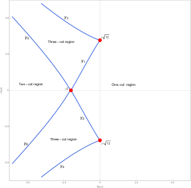
Figure 2. Phase diagram for the geometry of $\mu_{t}$, courtesy of Roozbeh Gharakhloo.

It is well understood that the large $n$ behavior of $P_{n}(z;t,N),\gamma_{n}^{2}(t,N)$ (and consequently the partition function $Z_{n}(t,N)$ and the free energy $F_{n}(t,N)$) heavily depends on the choice of the complex parameter $t$, and particularly on the geometry of the attracting set for the zeros of $P_{n}(z;t,N)$. The corresponding phase diagram, shown in Figure 2, was obtained computationally in [BT], and a rigorous description followed in [BGM]. The regions labeled one-, two-, and three-cuts correspond to parameters $t$ where the measure $\mu_{t}$ defined by $n^{-1}\sum_{z\mathrel{\mathop{\mathchar 58\relax}}\ P_{n}(z)=0}\delta_{z}\stackrel{{\scriptstyle*}}{{\to}}\mu_{t}$ is supported on one, two, or three analytic arcs, respectively. Henceforth we will label these regions $\mathcal{O}_{1},\mathcal{O}_{2},\mathcal{O}_{3}$, respectively, and delay a more precise definition to Section 4. The striking resemblance between Figures 1, 2 is no accident! Heuristically, given a measure of the form ${\mathrm{e}}^{-NV(z)}{\mathrm{d}}z$, one can prove that non-Hermitian orthogonal polynomials satisfy $\text{deg}P_{n}=n$ for all $n$ large enough in the one-cut regime. This implies a lack of zeros of $H_{n-1}(t,N)$ (and hence poles of $\gamma_{n}^{2}(t,N)$). In the setting of the Quartic Model, asymptotics of $P_{n}$ have been obtained when $t\geq-2$ in [BI] and extended to $t\in\mathcal{O}_{1}$ in [BGM]. It is slightly more surprising that the region $\mathcal{O}_{2}$ is also free of zeros of $H_{n-1}(t,N)$, but this is indeed the case and is basically due to the symmetry of (1.6). We will prove this as well as asymptotics of $P_{n}(z;t,N),\gamma_{n}^{2}(t,N)$ in Section 5 (see Theorems 4.13, 4.17, respectively). A by-product of this analysis is that $(f_{0},f_{1},f_{2})_{n,0,0}(x)$ is asymptotically free of poles in $2^{-1/2}n^{1/2}\mathcal{O}_{2}$, as can be seen from the following corollary.

Corollary 1.5.

Let $(f_{0})_{n,m,k},(f_{1})_{n,m,k},(f_{2})_{n,m,k}$ be the Bäcklund iterates of the solution of ($\textnormal{P}^{\textnormal{sym}}_{IV}$) with parameters $(\alpha_{0},\alpha_{1},\alpha_{2})=(0,\frac{1}{2},\frac{1}{2})$ given by

$$(f_{0}(x),f_{1}(x),f_{2}(x))_{0,0,0}=\left(0,\frac{\varphi^{\prime}(x)}{\varphi(x)},2x-\frac{\varphi^{\prime}(x)}{\varphi(x)}\right),\quad\varphi(x)={\mathrm{e}}^{x^{2}/2}D_{-1/2}(\sqrt{2}x).$$

Then, as $n\to\infty$,

(1.31) $$2^{1/2}n^{-1/2}(f_{0})_{n,0,0}(2^{-1/2}n^{1/2}x) =x+\sqrt{x^{2}-4}+\mathcal{O}\left(\frac{1}{n}\right),$$

$$2^{1/2}n^{-1/2}(f_{1})_{n,0,0}(2^{-1/2}n^{1/2}x) =\dfrac{4}{x+\sqrt{x^{2}-4}}+\mathcal{O}\left(\frac{1}{n}\right),$$

$$2^{1/2}n^{-1/2}(f_{2})_{n,0,0}(2^{-1/2}n^{1/2}x) =\mathcal{O}\left(\frac{1}{n}\right),$$

and

(1.32) $$2^{1/2}n^{-1/2}\sigma_{n-1,0,0}(2^{-1/2}n^{1/2}x) =\dfrac{x-\sqrt{x^{2}-4}}{2}+\mathcal{O}\left(\frac{1}{n}\right),$$

$$2^{1/2}n^{-1/2}\sigma_{n-1,-1,0}(2^{-1/2}n^{1/2}x) =\dfrac{-x+\sqrt{x^{2}-4}}{2}+\mathcal{O}\left(\frac{1}{n}\right),$$

locally uniformly for $x\in\mathcal{O}_{2}$. In all cases, $\sqrt{x^{4}-4}$ is the branch analytic in ${\mathbb{C}}\setminus[-2,2]$ and satisfies $\sqrt{x^{2}-4}\sim-x$ as $x\to\infty$.

Remark 1.6.

An analogous model, known as the Cubic Model was also investigated in [BIPZ] and is connected with the enumeration of 3-valent graphs on Riemann surfaces. This corresponds to the specialization $\mathcal{V}(x)=\frac{1}{2}x^{2}+\frac{u}{3}x^{3}$ in (1.22), and results in the replacement of the potential $V(z)$ by the polynomial $\tilde{V}(z)=z^{3}/3+tz^{2}/2$. The astute reader might immediately object since integrals in (1.5) and the total mass of (1.22) are not convergent. To make sense of the model, one needs to deform the contour of integration to the complex plane, at which point the model loses its interpretation as an ensemble of random Hermitian matrices. However, the enumeration property still holds as was shown in [BD]. Later, the connection between the partition function and solutions of Painlevé-II was established in [BBDY] and further expanded on in [BBDY2]. In many ways, this manuscript can be viewed as the analog of [BBDY] for the Quartic Model.

We point out that the phase diagram contains three points that are of particular interest in the mathematical physics literature because of the presence of “critical phenomenon.” At the level of polynomials $P_{n}$, this manifests itself in non-generic asymptotic formulas. Asymptotic formulas in the double-scaling regime $t\to t_{cr}^{II}=-2$ were obtained in [MR1715324] and involve particular solutions of Painlevé-II. An analogous result, but involving solutions to Painlevé-I, when $t\to t_{cr}^{I}=\pm{\mathrm{i}}\sqrt{12}$ were obtained in [DK].

In the finite $n$ setting, it was already known to Shohat [Shohat] that the recurrence coefficients of polynomials orthogonal with respect to measures of the form in (1.5) are solutions to integrable equations. Fokas, Its, and Kitaev realized that the recurrence coefficients $\gamma_{n}^{2}(t,N)$ satisfy both continuous and discrete Painlevé equations [FIK, FIK2] (see also Magnus’ work[Magnus, Magnus2]). The discrete equation in question is the discrete version of Painlevé-I and is given by

(1.33) $$\gamma_{n}^{2}(t,N)\left(t+\gamma_{n-1}^{2}(t,N)+\gamma_{n}^{2}(t,N)+\gamma_{n+1}^{2}(t,N)\right)=\dfrac{n}{N}.$$

This equation is known in the random matrix theory literature as the string equation, and is central to the analysis in [MR1715324], for example. While we will not use it here, we do mention some of its applications to our analysis in Section 6. A related family of orthogonal polynomials, known as the semi-classical Laguerre polynomials, also appears in the literature. These are polynomials $L_{n}(x;t,\ell)$ satisfying

(1.34) $$\int_{0}^{\infty}x^{k}L_{n}(x;t,\ell)x^{\ell}{\mathrm{e}}^{-\left(x^{2}+tx\right)}{\mathrm{d}}x=0\quad\text{for}\quad k=0,1,...,n-1.$$

These polynomials were the subject of study in [BV, FVZ, CJ], where the connection between their recurrence coefficients and special function solutions of ($\textnormal{P}_{IV}$) was established. It is not hard to imagine that polynomials $L_{n}$ and $P_{n}$ are related, see Proposition A.2 in the Appendix.

1.5. Overview of the rest of the paper

In Section 2, we recall various properties of the symmetric and Hamiltonian formulations of ($\textnormal{P}_{IV}$), their various Bäcklund transformations, and define $\tau_{n,m,k}(x),\sigma_{n,m,k}(x)$. In Section 3, we derive some auxiliary identities and prove Lemma 1.2 and Theorem 1.3. In Section 4 we introduce various notions that will be essential to the asymptotic analysis of $P_{n},\gamma_{n}^{2}$ and state asymptotic formulas for $P_{n}$ in Theorem 4.13 and for $h_{n},\gamma_{n}^{2}$ in Theorem 4.17 and deduce Corollary 1.5. Section 5 is dedicated to the proofs of Theorems 4.13, 4.17. We highlight various open questions and directions to extend this work in Section 6. Finally, we record some observations regarding $P_{n}$ in the Appendix A.

1.6. Acknowledgements

It is the author’s pleasure to thank Pavel Bleher and Maxim Yattselev for introducing me to the Cubic and Quartic Models, Alfredo Deaño and Peter Miller for introducing me to special function solutions of Painlevé equations and the theory surrounding them, Pavel Bleher, Roozbeh Gharakhloo, and Ken McLaughlin for patiently explaining their work [BGM] to me, and Maurice Duits, Nathan Hayford, and Roger Van Peski for their helpful comments while writing this manuscript. A special thank you to Andrei Prokhorov, who was my office mate at University of Michigan and is infinitely willing to discuss mathematics.

2. Painlevé-IV and its Bäcklund Transformations

We start this section by closely examining Theorem 1.1. While the forward direction of (1.1) can be readily checked, it is less clear that given $u(x)$ which solves ($\textnormal{P}_{IV}$), one can construct a triple $(f_{0}(x),f_{1}(x),f_{2}(x))$ which solves ($\textnormal{P}^{\textnormal{sym}}_{IV}$). This can be seen from the Hamiltonian formulation of ($\textnormal{P}_{IV}$). Indeed, letting

(2.1) $$H_{IV}(x;p,q;\alpha_{0},\alpha_{1},\alpha_{2})=(2p-q-2x)pq-2\alpha_{1}p-\alpha_{2}q,$$

we arrive at the system

(2.2) $$\mathinner{\dfrac{\operatorname{d\!}{}q}{\operatorname{d\!}{x}}}=\mathinner{\dfrac{\partial{}H_{IV}}{\partial{p}}} =q(4p-q-2x)-2\alpha_{1},$$

(2.3) $$\mathinner{\dfrac{\operatorname{d\!}{}p}{\operatorname{d\!}{x}}}=-\mathinner{\dfrac{\partial{}H_{IV}}{\partial{q}}} =p(2q-2p+2x)+\alpha_{2}.$$

One can readily check that eliminating $p(x)$ from (2.2), (2.3) reveals that $q(x)$ solves ($\textnormal{P}_{IV}$) with parameters (1.4). On the other hand, given a solution of ($\textnormal{P}_{IV}$), $u(x)$, the Hamiltonian system $\{H,p,q\}$ is determined by $q(x)=u(x)$ and

(2.4) $$p(x)=\dfrac{1}{4q(x)}\left(2\alpha_{1}+2xq(x)+q^{2}(x)+q^{\prime}(x)\right).$$

Letting

(2.5) $$f_{1}(x)=-q(x),\quad f_{2}(x)=2p(x),\quad f_{0}(x)=2x+q(x)-2p(x),$$

shows that (2.2), (2.3) are equivalent to the last two equations in ($\textnormal{P}^{\textnormal{sym}}_{IV}$). Since (2.5) clearly satisfy the constraint (1.3), this implies that the functions (2.5) satisfy the first equation in ($\textnormal{P}^{\textnormal{sym}}_{IV}$).

Remark 2.1.

The reader might wonder how, given a solution $(u(x),\Theta_{0},\Theta_{\infty})$ one might determine the parameters $\alpha_{0},\alpha_{1},\alpha_{2}$. From (1.1) and (1.4), it is clear that one must choose $\Theta_{0}=\pm 2\alpha_{j}$ for some $j=0,1,2$. Once this choice is made, the remaining parameters are uniquely determined by the conditions

$$\alpha_{j-1}+\alpha_{j+1} =1-\alpha_{j},$$

$$\alpha_{j-1}-\alpha_{j+1} =2\Theta_{\infty}-1.$$

Changing our choice $\alpha_{j}\mapsto-\alpha_{j}$ amounts to applying the Bäcklund transformation $s_{j}^{-1}$ which is introduced in the next section.

2.1. Bäcklund transformations for the system ($\textnormal{P}^{\textnormal{sym}}_{IV}$)

Much of the discussion below is contained in [NY], see also the already mentioned [FW]. We begin by recording an obvious symmetry

(2.6) $$\pi(f_{j}(x))=f_{j-1}(x),\quad\pi(\alpha_{j})=\alpha_{j-1}$$

leaves the system ($\textnormal{P}^{\textnormal{sym}}_{IV}$) and condition (1.3) invariant.

Remark 2.2.

Due to this symmetry of ($\textnormal{P}^{\textnormal{sym}}_{IV}$), a given solution of ($\textnormal{P}_{IV}$) can be identified with the negative of any one function in the triple $(f_{0}(x),f_{1}(x),f_{2}(x))$. Moving forward, we will always write $u(x)=-f_{1}(x)$ to avoid ambiguity.

More nontrivial transformations exist, and they are summarized by the proposition below.

Proposition 2.3.

Let $\{\alpha_{j}\}_{j=0}^{2}$ and $\{f_{j}(x)\}_{j=0}^{2}$ be as above. Define the Cartan matrix $A$ and orientation matrix $U$ by

(2.7) $$\mathbf{A}=[a_{ij}]_{i,j=0}^{2}=\left[\begin{array}[]{rrr}2&-1&-1\\ -1&2&-1\\ -1&-1&2\end{array}\right],\quad\mathbf{U}=[u_{ij}]_{i,j=0}^{2}=\left[\begin{array}[]{rrr}0&1&-1\\ -1&0&1\\ 1&-1&0\end{array}\right],$$

and consider the functions given by transformations

(2.8) $$g_{ij}(x)\mathrel{\mathop{\mathchar 58\relax}}=s_{i}(f_{j}(x))=f_{j}(x)+u_{ij}\dfrac{2\alpha_{i}}{f_{i}(x)},\quad i,j\in\{0,1,2\}.$$

Then the triple $(g_{i0},g_{i1},g_{i2})$ satisfy (1.3) and solve ($\textnormal{P}^{\textnormal{sym}}_{IV}$) with parameters $(\beta_{i0},\beta_{i1},\beta_{i2})$ given by

(2.9) $$\beta_{ij}=s_{i}(\alpha_{j})\mathrel{\mathop{\mathchar 58\relax}}=\alpha_{j}-a_{ij}\alpha_{i}.$$

Remark 2.4.

One can observe that the lines $\alpha_{j}=k\in{\mathbb{Z}}$ define a triangular lattice on the plane (1.2) which is associated with an $A_{2}^{(1)}$ root system whose roots, with a slight abuse of notation, are given by

(2.10) $$\boldsymbol{\alpha}_{0}=\begin{bmatrix}0&-1&1\end{bmatrix}^{T},\quad\boldsymbol{\alpha}_{1}=\begin{bmatrix}1&0&-1\end{bmatrix}^{T},\quad\boldsymbol{\alpha}_{2}=\begin{bmatrix}-1&1&0\end{bmatrix}^{T}.$$

The reflection across $\boldsymbol{\alpha}_{j}$ is then given by

(2.11) $$s_{i}(\boldsymbol{\alpha}_{j})=\boldsymbol{\alpha}_{j}-a_{ij}\boldsymbol{\alpha}_{i},$$

where $a_{ij}$ are the elements of $\mathbf{A}$ in (2.7). This connection is the source of the names of the matrices $\mathbf{A},\mathbf{U}$, but will not be used in the sequel.

It can be checked that $s_{j}$, when acting on triples $(f_{0}(x),f_{1}(x),f_{2}(x))$, are involutions. Indeed,

(2.12) $$s_{0}^{2}(f_{0}(x),f_{1}(x),f_{2}(x)) =s_{0}\left(f_{0}(x),f_{1}(x)+\dfrac{2\alpha_{0}}{f_{0}(x)},f_{2}(x)-\dfrac{2\alpha_{0}}{f_{0}(x)}\right)$$

(2.13) $$=\left(f_{0}(x),f_{1}(x)+\dfrac{2\alpha_{0}}{f_{0}(x)}+\dfrac{2s_{0}(\alpha_{0})}{f_{0}(x)},f_{2}(x)-\dfrac{2\alpha_{0}}{f_{0}(x)}-\dfrac{2s_{0}(\alpha_{0})}{f_{0}(x)}\right)$$

(2.14) $$=(f_{0}(x),f_{1}(x),f_{2}(x)).$$

In fact, slightly more involved (but direct) computations reveal that $s_{j},\sigma$ satisfy

(2.15) $$s_{j}^{2}=1,\quad(s_{j}s_{j+1})^{3}=1,\quad\pi^{3}=1,\quad\pi s_{j}=s_{j+1}\pi.$$

Moving forward, we will think of $s_{i},\sigma$ as acting on a triples of functions where we denote by

$$s_{j}(f_{0}(x),f_{1}(x),f_{2}(x))\mathrel{\mathop{\mathchar 58\relax}}=\left(s_{j}(f_{0}(x)),s_{j}(f_{1}(x)),s_{j}(f_{2}(x))\right)$$

a triple which solves ($\textnormal{P}^{\textnormal{sym}}_{IV}$) with parameters

$$s_{j}(\alpha_{0},\alpha_{1},\alpha_{2})=(s_{j}(\alpha_{0}),s_{j}(\alpha_{1}),s_{j}(\alpha_{2})).$$

We now construct three transformations:

(2.16) $$T_{1}\mathrel{\mathop{\mathchar 58\relax}}=\pi s_{2}s_{1},\quad T_{2}\mathrel{\mathop{\mathchar 58\relax}}=s_{1}\pi s_{2},\quad T_{3}\mathrel{\mathop{\mathchar 58\relax}}=s_{2}s_{1}\pi.$$

The action of $T_{i}$ on parameters $\alpha_{j}$ is summarized in the Table 1. One might guess from this table that (with indices interpreted cyclically)

(2.17) $$T_{j}T_{j+1}T_{j+2}=1\quad\text{for}\quad j=1,2,3,$$

and this is indeed the case as can be verified using (2.15). We verify one such identity and leave the rest to the reader:

$$T_{1}T_{2}T_{3}=\pi s_{2}s_{1}s_{1}\pi s_{2}s_{2}s_{1}\pi=\pi s_{2}\pi s_{1}\pi=s_{0}\pi^{3}s_{0}=1.$$

Similarly, one can verify that $T_{i}T_{j}=T_{j}T_{i}$ for any $i,j\in\{1,2,3\}$ and the identities

(2.18) $$T_{j+1}=\pi T_{j}\pi^{-1}.$$

Since $s_{j},\pi$ are invertible, it follows that $T_{j}$ are invertible and

(2.19) $$T_{1}^{-1}=s_{1}s_{2}\pi^{-1},\quad T_{2}^{-1}=s_{2}\pi^{-1}s_{1},\quad T_{3}^{-1}=\pi^{-1}s_{1}s_{2}.$$

We now investigate the effect of $T_{i}$ on a given solution of ($\textnormal{P}_{IV}$); since the transformations $T_{j}$ are related by (2.18), we focus our attention on $T_{1}$, which will generate the family of solutions we are interested in. Given a triple $(f_{0}(x),f_{1}(x),f_{2}(x))$ which solves ($\textnormal{P}^{\textnormal{sym}}_{IV}$), then

(2.20) $$T_{1} (f_{0}(x),f_{1}(x),f_{2}(x))=\pi s_{2}\left(g_{10}(x),g_{11}(x),g_{12}(x)\right)$$

$$=\pi\left(g_{10}(x)+u_{20}\dfrac{2s_{1}(\alpha_{2})}{g_{12}(x)},g_{11}(x)+u_{21}\dfrac{2s_{1}(\alpha_{2})}{g_{12}(x)},g_{12}(x)+u_{22}\dfrac{2s_{1}(\alpha_{2})}{g_{12}(x)}\right)$$

$$=\pi\left(g_{10}(x)+\dfrac{2(\alpha_{1}+\alpha_{2})}{g_{12}(x)},g_{11}(x)-\dfrac{2(\alpha_{1}+\alpha_{2})}{g_{12}(x)},g_{12}(x)\right)$$

$$=\left(g_{12}(x),g_{10}(x)+\dfrac{2(\alpha_{1}+\alpha_{2})}{g_{12}(x)},g_{11}(x)-\dfrac{2(\alpha_{1}+\alpha_{2})}{g_{12}(x)}\right)$$

$$=\left(f_{2}(x)+\dfrac{2\alpha_{1}}{f_{1}(x)},f_{0}(x)-\dfrac{2\alpha_{1}}{f_{1}(x)}+\dfrac{2(\alpha_{1}+\alpha_{2})f_{1}(x)}{(f_{1}f_{2})(x)+2\alpha_{1}},f_{1}(x)-\dfrac{2(\alpha_{1}+\alpha_{2})f_{1}(x)}{(f_{1}f_{2})(x)+2\alpha_{1}}\right).$$

solves ($\textnormal{P}^{\textnormal{sym}}_{IV}$) with parameters $(\alpha_{0}-1,\alpha_{1}+1,\alpha_{2})$. In a similar fashion, one can check that

(2.21) $$T_{1}^{-1}(f_{0}(x),f_{1}(x),f_{2}(x))\\ =\left(f_{1}(x)+\dfrac{2\alpha_{0}}{f_{0}(x)}-\dfrac{2(\alpha_{0}+\alpha_{2})f_{0}(x)}{(f_{0}f_{2})(x)-2\alpha_{0}},f_{2}(x)-\dfrac{2\alpha_{0}}{f_{0}(x)},f_{0}(x)+\dfrac{2(\alpha_{0}+\alpha_{2})f_{0}(x)}{(f_{0}f_{2})(x)-2\alpha_{0}}\right)$$

solves ($\textnormal{P}^{\textnormal{sym}}_{IV}$) with parameters $(\alpha_{0}+1,\alpha_{1}-1,\alpha_{2})$. Henceforth, we will use the notation $T_{1}(f_{j}(x)),T_{1}^{-1}(f_{j}(x))$ to denote the $j$th entry of the hand side of (2.20), (2.21), respectively.

Remark 2.5.

It can occur (see Example 1 below) that either $f_{1}(x)=0$ or $(f_{1}f_{2})(x)+2\alpha_{1}=0$ holds identically, which causes an indeterminacy in (2.20). We highlight that the requirement that $T_{1}(f_{0},f_{1},f_{2})$ be determinate is really a condition on $f_{1}$. Indeed, given that $(f_{0},f_{1},f_{2})$ satisfies ($\textnormal{P}^{\textnormal{sym}}_{IV}$), (1.3), $f_{2}$ is given in terms of $f_{1}$ as (this is exactly (2.4))

$$f_{2}(x)=\dfrac{1}{2f_{1}(x)}\left(-2\alpha_{1}+2xf_{1}(x)-f_{1}^{2}(x)+f_{1}^{\prime}(x)\right).$$

Hence, for $T_{1}(f_{0},f_{1},f_{2})$ to be determinate we must require $f_{1}(x)\not\equiv 0$ and

$$f_{1}^{\prime}(x)-f_{1}^{2}(x)+2xf_{1}(x)+2\alpha_{1}\not\equiv 0.$$

We will later show (see Proposition 2.12 below) that the particular family of solutions we study in this paper is determinate.

2.2. Bäcklund transformations for ($\textnormal{P}_{IV}$)

On the level of the parameters $(\Theta_{0},\Theta_{\infty})$, if $u(x)=-f_{1}(x)$ solves ($\textnormal{P}_{IV}$) with parameters $\alpha=\alpha_{0}-\alpha_{2}=2\Theta_{\infty}-1$ and $\beta=-2\alpha_{1}^{2}=-8\Theta_{0}^{2}$, then letting $\alpha_{1}=2\Theta_{0}$ and $\alpha_{0},\alpha_{2}$ be the corresponding parameters (see Remark 2.1) then $u_{\searrow}(x)\mathrel{\mathop{\mathchar 58\relax}}=-T_{1}(f_{1}(x))$ solves ($\textnormal{P}_{IV}$) with parameters

$${\Theta}_{\infty,\searrow}=\Theta_{\infty}-\frac{1}{2},\quad{\Theta}_{0,\searrow}=\Theta_{0}+\frac{1}{2}.$$

It follows from (2.20) that

(2.22) $$u_{\searrow}(x)=\dfrac{(2\alpha_{1})^{2}-8(\alpha_{1}+\alpha_{2})u^{2}(x)-4x^{2}u^{2}(x)-4xu^{3}(x)-u^{4}(x)-4\alpha_{1}u^{\prime}(x)+u^{\prime}(x)^{2}}{2u(x)(-2\alpha_{1}+2xu(x)+u^{2}(x)+u^{\prime}(x))},$$

which, upon recalling the definitions of $\alpha_{i}$’s and the constraint (1.2), agrees with [BM]*Equation 3.50. If, on the other hand, we set $\alpha_{1}=-2\Theta_{0}$ and $\alpha_{0},\alpha_{2}$ be the corresponding parameters, then $u_{\swarrow}(x)\mathrel{\mathop{\mathchar 58\relax}}=-T_{1}(f_{1}(x))$ solves ($\textnormal{P}_{IV}$) with parameters

$$\Theta_{\infty,\swarrow}=\Theta_{\infty}-\frac{1}{2},\quad\Theta_{0,\swarrow}=\Theta_{0}-\frac{1}{2}.$$

The function $u_{\swarrow}$ is again given by the right hand side of (2.22) which, upon recalling the definitions of $\alpha_{i}$’s and the constraint (1.2), agrees with [BM]*Equation 3.49. We can extract two more Bäcklund transformations for ($\textnormal{P}_{IV}$) from the expression (2.21); letting $\alpha_{1}=2\Theta_{0}$, $\alpha_{0},\alpha_{2}$ be the corresponding parameters, and $u_{\nwarrow}(x)\mathrel{\mathop{\mathchar 58\relax}}=-T_{1}^{-1}(f_{1})$, then it follows from (2.21) that

(2.23) $$u_{\nwarrow}(x)=\dfrac{(2\alpha_{1})^{2}+8\alpha_{0}u^{2}(x)-4x^{2}u^{2}(x)-4xu^{3}(x)-u^{4}(x)+4\alpha_{1}u^{\prime}(x)+u^{\prime}(x)^{2}}{2u(x)(-2\alpha_{1}+2xu(x)+u^{2}(x)-u^{\prime}(x))},$$

which agrees with [BM]*Equation 3.51. In a similar fashion to the previous paragraph, if instead we set $\alpha_{1}=-2\Theta_{0}$, $\alpha_{0},\alpha_{2}$ be the corresponding parameters, and $u_{\nearrow}(x)\mathrel{\mathop{\mathchar 58\relax}}=-T_{1}^{-1}(f_{1})$, then we find that $u_{\nearrow}(x)$ is given by the right hand side of (2.23). Plugging in the the definitions of $\alpha_{i}$’s and the constraint (1.2), we arrive at [BM]*Equation 3.48.

Remark 2.6.

We pause here to highlight the result of the above calculation. A given solution of ($\textnormal{P}_{IV}$) $(u(x),\Theta_{0},\Theta_{\infty})$ can be embedded into two distinct pairs of solutions of ($\textnormal{P}^{\textnormal{sym}}_{IV}$) by setting $u(x)=-f_{1}(x)$ and making the choice $\alpha_{1}=\pm 2\Theta_{0}$. This then fixes the triple $(f_{0},f_{1},f_{2})$ uniquely (see Remark 2.1). Of course these are not the only triples where the function $u(x)$ appears as $-f_{1}(x)$ since one could act on this triple by $s_{1}$. Furthermore, one could write triples for which $u(x)=-f_{2}(x)$ or $u(x)=-f_{0}(x)$ by acting on $(f_{0},f_{1},f_{2})$ by $\pi^{\pm 1}$. As stated in Remark 2.2, given a solution $(u(x),\Theta_{0},\Theta_{\infty})$, we will prefer to set $u(x)=-f_{1}(x)$.

2.3. The $\sigma$-form of Painlevé-IV

Recalling (2.1), (2.5), we define $\sigma(x;\alpha_{0},\alpha_{1},\alpha_{2})\equiv\sigma(x)$ by

(2.24) $$\sigma(x)=H(x;p(x),q(x);\alpha_{0},\alpha_{1},\alpha_{2})=\frac{1}{2}(f_{0}f_{1}f_{2})(x)+\alpha_{2}f_{1}(x)-\alpha_{1}f_{2}(x).$$

It follows (see [FW]*Proposition 4) that $\sigma(x)$ satisfies the Jimbo-Miwa-Okamoto $\sigma$-form of $\textnormal{P}_{IV}$:

(2.25) $$\left(\mathinner{\dfrac{\operatorname{d\!}{{}^{2}}\sigma}{\operatorname{d\!}{x^{2}}}}\right)^{2}-4\left(x\mathinner{\dfrac{\operatorname{d\!}{}\sigma}{\operatorname{d\!}{x}}}-\sigma(x)\right)+4\mathinner{\dfrac{\operatorname{d\!}{}\sigma}{\operatorname{d\!}{x}}}\left(\mathinner{\dfrac{\operatorname{d\!}{}\sigma}{\operatorname{d\!}{x}}}+2\alpha_{1}\right)\left(\mathinner{\dfrac{\operatorname{d\!}{}\sigma}{\operatorname{d\!}{x}}}-2\alpha_{2}\right)=0.$$

Remark 2.7.

The function $\sigma(x)$ can be directly related to a solution of ($\textnormal{P}_{IV}$). In one direction, given $(u(x),\Theta_{0},\Theta_{\infty})$ which solves ($\textnormal{P}_{IV}$), using (2.4) and (2.5) immediately yields an expression for $\sigma(x)$ in terms of $u(x)$. On the other hand, letting $p,q$ be as in (2.5), it follows from (2.2), (2.3) and the last two equations in ($\textnormal{P}^{\textnormal{sym}}_{IV}$) that

(2.26) $$\mathinner{\dfrac{\operatorname{d\!}{}\sigma}{\operatorname{d\!}{x}}} =f_{1}f_{2},$$

(2.27) $$\mathinner{\dfrac{\operatorname{d\!}{{}^{2}}\sigma}{\operatorname{d\!}{x^{2}}}} =f_{1}f_{2}(f_{2}-f_{1})+2\alpha_{2}f_{1}+2\alpha_{1}f_{2}.$$

Using (2.26), (2.24) in (2.27) yields

(2.28) $$\mathinner{\dfrac{\operatorname{d\!}{{}^{2}}\sigma}{\operatorname{d\!}{x^{2}}}}=2\alpha_{2}f_{1}(x)-(\sigma f_{1})(x)+\dfrac{1}{f_{1}(x)}\mathinner{\dfrac{\operatorname{d\!}{}\sigma}{\operatorname{d\!}{x}}}\left(\mathinner{\dfrac{\operatorname{d\!}{}\sigma}{\operatorname{d\!}{x}}}+2\alpha_{1}\right).$$

To calculate the last term, we note that using (2.24) and (1.3) in (2.24) implies

(2.29) $$\dfrac{1}{f_{1}(x)}\mathinner{\dfrac{\operatorname{d\!}{}\sigma}{\operatorname{d\!}{x}}}\left(\mathinner{\dfrac{\operatorname{d\!}{}\sigma}{\operatorname{d\!}{x}}}+2\alpha_{1}\right)=(2x-f_{1}(x))\mathinner{\dfrac{\operatorname{d\!}{}\sigma}{\operatorname{d\!}{x}}}+2\alpha_{2}f_{1}(x)-2\sigma(x).$$

Putting this together yields a solution of ($\textnormal{P}_{IV}$) given by

$$u(x)=-f_{1}(x)=\dfrac{\sigma^{\prime\prime}(x)-2x\sigma^{\prime}(x)+2\sigma(x)}{2\sigma^{\prime}(x)-4\alpha_{2}}.$$

In the sequel, given a Bäcklund transformation $B\in\langle s_{0},s_{1},s_{2},\pi\rangle$, we define (sticking with the abuse of notation in Footnote 5)

(2.30) $$B(\sigma(x))\mathrel{\mathop{\mathchar 58\relax}}=\frac{1}{2}\left(B(f_{0})B(f_{1})B(f_{2})\right)(x)+B(\alpha_{2})B(f_{1})(x)-B(\alpha_{1})B(f_{2})(x),$$

A direct computation using (2.24), (1.2), and (1.3) shows that

(2.31) $$s_{0}(\sigma(x)) =\sigma(x)+\dfrac{2\alpha_{0}}{f_{0}(x)},$$

$$s_{1}(\sigma(x)) =\sigma(x)+2\alpha_{1}x,$$

$$s_{2}(\sigma(x)) =\sigma(x)-2\alpha_{2}x,$$

$$\pi(\sigma(x)) =\sigma(x)-f_{1}(x)+2\alpha_{1}x,$$

$$\pi^{-1}(\sigma(x))=\pi^{2}(\sigma(x)) =\sigma(x)+f_{2}(x)-2\alpha_{2}x.$$

Using these we find that

(2.32) $$T_{1}(\sigma(x)) =\sigma(x)-s_{2}s_{1}(f_{1}(x))=\sigma(x)-T_{1}(f_{2}(x)),$$

(2.33) $$T_{1}^{-1}(\sigma(x)) =\sigma(x)+f_{2}(x).$$

While they can be computed directly using (2.31), relation (2.32) allows us to deduce analogous identities for $T_{2},T_{3}$ by using (2.31) and (2.18) and we find

(2.34) $$T_{2}(\sigma(x))-\sigma(x)=2x-s_{2}(f_{1}(x)),$$

(2.35) $$T_{3}(\sigma(x))-\sigma(x)=-f_{1}(x).$$

The final object which will be important for our investigation is the so-called $\tau$-function, defined up to a constant of integration to be fixed later (see Proposition 2.8) by

(2.36) $$\sigma(x)=\mathinner{\dfrac{\operatorname{d\!}{}}{\operatorname{d\!}{x}}}\log\tau(x).$$

The Bäcklund iterates of $\tau$, $B(\tau(x))$, $B\in\langle s_{0},s_{1},s_{2},\pi\rangle$, are defined analogously to (2.30) by

(2.37) $$B(\sigma(x))=\mathinner{\dfrac{\operatorname{d\!}{}}{\operatorname{d\!}{x}}}\log B(\tau(x)).$$

Plugging this into (2.32) we see that

(2.38) $$-T_{1}(f_{2}(z))=\mathinner{\dfrac{\operatorname{d\!}{}}{\operatorname{d\!}{t}}}\log\left(\dfrac{T_{1}(\tau(x))}{\tau(x)}\right).$$

A remarkable fact first observed by Okamoto, cf. [O]*Proposition 3.5, is that the difference $T_{1}(f_{2}(x))-f_{2}(x)$ can be written as a derivative. More precisely, the third entry in the final expression in (2.20) and ($\textnormal{P}^{\textnormal{sym}}_{IV}$) imply

(2.39) $$T_{1}(f_{2}(x))-f_{2}(x) =-\mathinner{\dfrac{\operatorname{d\!}{}}{\operatorname{d\!}{x}}}\log\left((f_{1}f_{2})(x)+2\alpha_{1}\right),$$

and by applying identity (2.39) to the triple $T_{1}(f_{0},f_{1},f_{2})$ we get

(2.40) $$f_{2}(x)-T_{1}^{-1}(f_{2}(x))=-\mathinner{\dfrac{\operatorname{d\!}{}}{\operatorname{d\!}{x}}}\log\left((f_{0}f_{2})(x)-2\alpha_{0}\right).$$

We record one more identity of this type here; by recalling that (2.18) we arrive at

(2.41) $$f_{1}(x)-T_{3}^{-1}(f_{1}(x))=-\mathinner{\dfrac{\operatorname{d\!}{}}{\operatorname{d\!}{x}}}\log\left((f_{1}f_{2})(x)-2\alpha_{2}\right).$$

These identities will be crucial ingredients in deriving the Toda equations.

2.4. Bäcklund iterates and the Toda equation(s)

We will be interested in families of solutions of ($\textnormal{P}_{IV}$) generated by iterating $T_{1},T_{2},T_{3}$ and their inverses. To this end, recall our notation $g_{n,m,k}(x)\mathrel{\mathop{\mathchar 58\relax}}=T_{3}^{k}T_{2}^{m}T_{1}^{n}(g_{0}(x))$ for all relevant functions and $n,m,k\in{\mathbb{Z}}$ ($T_{j}$’s commute so the order of application is immaterial). When iterating a single $T_{j}$, we will slightly abuse notation (hopefully without causing confusion) by dropping the fixed indices.

Proposition 2.8 ([O], see also [FW]*Proposition 5).

Fix $m,k\in{\mathbb{Z}}$. For all $n\in{\mathbb{Z}}$, let $\tilde{\tau}_{n,m,k}(x)\mathrel{\mathop{\mathchar 58\relax}}={\mathrm{e}}^{x^{2}(\alpha_{1}+n)}\tau_{n,m,k}(x)$. Then, functions $\{\tilde{\tau}_{n}\}_{n\in{\mathbb{Z}}}$ satisfy the Toda equation:

(2.42) $$\mathinner{\dfrac{\operatorname{d\!}{{}^{2}}}{\operatorname{d\!}{x^{2}}}}\log\tilde{\tau}_{n,m,k}(x)=\dfrac{\tilde{\tau}_{n+1,m,k}(x)\tilde{\tau}_{n-1,m,k}(x)}{\tilde{\tau}^{2}_{n,m,k}(x)}.$$

Proof.

We start by writing $\tilde{\tau}_{n}(x)=\tilde{\tau}_{n,m,k}(x)$ noting that

(2.43) $$\mathinner{\dfrac{\operatorname{d\!}{}}{\operatorname{d\!}{x}}}\log\dfrac{\tilde{\tau}_{n+1}(x)\tilde{\tau}_{n-1}(x)}{\tilde{\tau}^{2}_{n}(x)}=\mathinner{\dfrac{\operatorname{d\!}{}}{\operatorname{d\!}{x}}}\log\dfrac{{\tau}_{n+1}(x){\tau}_{n-1}(x)}{{\tau}^{2}_{n}(x)}=\sigma_{n+1}(x)+\sigma_{n-1}(x)-2\sigma_{n}(x)\\ =(\sigma_{n+1}(x)-\sigma_{n}(x))-(\sigma_{n}(x)-\sigma_{n-1}(x)).$$

Now, writing $\sigma_{n+1}=T_{1}(\sigma_{n})$ and $\sigma_{n-1}=T_{1}^{-1}(\sigma_{n})$ and recalling (2.32), (2.33), and (2.39) yields

(2.44) $$\mathinner{\dfrac{\operatorname{d\!}{}}{\operatorname{d\!}{x}}}\log\dfrac{\tilde{\tau}_{n+1}(x)\tilde{\tau}_{n-1}(x)}{\tilde{\tau}^{2}_{n}(x)}=f_{2,n}(x)-T_{1}(f_{2,n}(x))=\mathinner{\dfrac{\operatorname{d\!}{}}{\operatorname{d\!}{x}}}\log((f_{1,n}f_{2,n})+2(\alpha_{1}+n)).$$

Finally, it follows from (2.26) that

(2.45) $$(f_{1,n}f_{2,n})+2(\alpha_{1}+n)=\mathinner{\dfrac{\operatorname{d\!}{}}{\operatorname{d\!}{x}}}(\sigma_{n}+2x(\alpha_{1}+n))=\mathinner{\dfrac{\operatorname{d\!}{{}^{2}}}{\operatorname{d\!}{x^{2}}}}\log\left(\tau_{n}{\mathrm{e}}^{x^{2}(\alpha_{1}+n)}\right).$$

Plugging (2.45) into (2.44), integrating and exponentiating yields

(2.46) $$\mathinner{\dfrac{\operatorname{d\!}{{}^{2}}}{\operatorname{d\!}{x^{2}}}}\log\tilde{\tau}_{n}(x)=K_{n,m,k}\dfrac{\tilde{\tau}_{n+1}(x)\tilde{\tau}_{n-1}(x)}{\tilde{\tau}^{2}_{n}(x)},\quad K_{n,m,k}\in{\mathbb{C}}\setminus\{0\}.$$

Now, we recall that $\tau_{n}$ is defined by (2.36) up to a constant of integration, and so we choose this constant so that $K_{n,m,k}=1$ for all $n\geq 0$. ∎

An even simpler statement holds for tau functions resulting from iterating $T_{2}$.

Proposition 2.9.

Fix $n,k\in{\mathbb{Z}}$. For all $n\in{\mathbb{Z}}$, the functions $\{{\tau}_{n,m,k}\}_{m\in{\mathbb{Z}}}$, there exist constants $K_{n,m,k}\in{\mathbb{C}}$ such that

(2.47) $$\mathinner{\dfrac{\operatorname{d\!}{{}^{2}}}{\operatorname{d\!}{x^{2}}}}\log{\tau}_{n,m,k}(x)=K_{n,m,k}\dfrac{{\tau}_{n,m+1,k}(x){\tau}_{n,m-1,k}(x)}{{\tau}^{2}_{n,m,k}(x)}.$$

Proof.

Beginning in the same was as in the proof of Proposition 2.8, we write

(2.48) $$\mathinner{\dfrac{\operatorname{d\!}{}}{\operatorname{d\!}{x}}}\log\dfrac{{\tau}_{m+1}(x){\tau}_{m-1}(x)}{{\tau}^{2}_{m}(x)}=(\sigma_{m+1}(x)-\sigma_{m}(x))-(\sigma_{m}(x)-\sigma_{m-1}(x)).$$

Writing $\sigma_{m+1}(x)=T_{2}(\sigma_{m}(x)),\ \sigma_{m-1}(x)=T_{2}^{-1}(\sigma_{m}(x))$, we now need identities analogous to (2.32), (2.33). Applying (2.34) to $\sigma_{m},T_{2}^{-1}(\sigma_{m})$ we find

$$\mathinner{\dfrac{\operatorname{d\!}{}}{\operatorname{d\!}{x}}}\log\dfrac{{\tau}_{m+1}(x){\tau}_{m-1}(x)}{{\tau}^{2}_{m}(x)}=s_{2}\left(T_{2}^{-1}(f_{1,m})\right)-s_{2}(f_{1,m})=T_{3}^{-1}(s_{2}(f_{1,m}))-s_{2}(f_{1,m}),$$

where the last equality follows by definition (2.16) of $T_{2},T_{3}$. Applying identity (2.41) with the triple $s_{2}(f_{0,m},f_{1,m},f_{2,m})$ and recalling (2.26), (2.36), we have

(2.49) $$\mathinner{\dfrac{\operatorname{d\!}{}}{\operatorname{d\!}{x}}}\log\dfrac{{\tau}_{m+1}(x){\tau}_{m-1}(x)}{{\tau}^{2}_{m}(x)}=\mathinner{\dfrac{\operatorname{d\!}{}}{\operatorname{d\!}{x}}}\log(f_{1,m}f_{2,m})=\mathinner{\dfrac{\operatorname{d\!}{}}{\operatorname{d\!}{x}}}\log\mathinner{\dfrac{\operatorname{d\!}{}\sigma_{m}}{\operatorname{d\!}{x}}}=\mathinner{\dfrac{\operatorname{d\!}{}}{\operatorname{d\!}{x}}}\log\mathinner{\dfrac{\operatorname{d\!}{{}^{2}}}{\operatorname{d\!}{x^{2}}}}\log\tau_{m}(x).$$

Integrating and exponentiating yields the result. ∎

Finally, for the sake of completeness, we record the Toda equation for iterates of $T_{3}$ and leave the proof (which essentially relies on (2.35) and (2.41)) as an exercise.

Proposition 2.10.

Fix $n,m\in{\mathbb{Z}}$ and let $\hat{\tau}_{n,m,k}(x)\mathrel{\mathop{\mathchar 58\relax}}={\mathrm{e}}^{x^{2}(k-\alpha_{2})}{\tau}_{n,m,k}$. For all $k\in{\mathbb{Z}}$, the functions $\{{\hat{\tau}}_{n,m,k}\}_{k\in{\mathbb{Z}}}$, there exist constants $C_{n,m,k}\in{\mathbb{C}}$ such that

(2.50) $$\mathinner{\dfrac{\operatorname{d\!}{{}^{2}}}{\operatorname{d\!}{x^{2}}}}\log{\hat{\tau}}_{n,m,k}(x)=C_{n,m,k}\dfrac{{\hat{\tau}}_{n,m+1,k}(x){\hat{\tau}}_{n,m-1,k}(x)}{{\hat{\tau}}^{2}_{n,m,k}(x)}.$$

Remark 2.11.

We pause here to make a few observations that will be useful in the sequel. It is known [GLS]*Theorem 4.1 that solutions of ($\textnormal{P}_{IV}$) can be continued to meromorphic function in ${\mathbb{C}}$. In particular, $\sigma(x)$ is a meromorphic function in ${\mathbb{C}}$. Furthermore, a dominant balance argument reveals that if $x_{0}$ is a pole of $\sigma(x)$, then

(2.51) $$\sigma(x)=\dfrac{1}{x-x_{0}}+\sigma_{0}-\dfrac{2}{3}(\alpha_{2}-\alpha_{1})(x-x_{0})+\mathcal{O}((x-x_{0})^{2})\quad\text{as}\quad x\to x_{0},\ \sigma_{0}\in{\mathbb{C}}.$$

In view of (2.36), (2.51) implies that roots of $\tau(x)$ are simple. Furthermore, since $\tilde{\tau}_{n,m,k}$ and $\tau_{n,m,k}$ share the same roots, roots of $\tilde{\tau}_{n,m,k}$ and $\hat{\tau}_{n,m,k}$ are simple. Writing (2.42) in the form

$$\tilde{\tau}_{n,m,k}^{\prime\prime}\tilde{\tau}_{n,m,k}-(\tilde{\tau}_{n,m,k}^{\prime})^{2}=\tilde{\tau}_{n+1,m,k}\tilde{\tau}_{n-1,m,k},$$

one can see that $\tilde{\tau}_{n,m,k}(x),\tilde{\tau}_{n+1,m,k}(x)$ (and hence ${\tau}_{n,m,k}(x),{\tau}_{n+1,m,k}(x)$) do not share any common roots. Similar considerations imply the analogous fact about $\tau_{n,m,k},\tau_{n,m+1,k}$ and $\tau_{n,m,k},\tau_{n,m,k+1}$.

2.5. Solutions in terms of special functions

It was already known (see, e.g., [O]*Section 5) that ($\textnormal{P}_{IV}$) possesses solutions which can be written in terms of classical special function. One can see this by requiring that ($\textnormal{P}_{IV}$) be compatible with a Riccati equation. Indeed, suppose we require that $u(x),$ besides satisfying ($\textnormal{P}_{IV}$) also satisfies

(2.52) $$\mathinner{\dfrac{\operatorname{d\!}{}u}{\operatorname{d\!}{x}}}=k_{2}(x)u^{2}(x)+k_{1}(x)u(x)+k_{0}(x).$$

Then, differentiating this equation and using ($\textnormal{P}_{IV}$) and comparing coefficients of the indicated terms implies

$$u^{3} \mathrel{\mathop{\mathchar 58\relax}} k_{2}^{2}(x) =1,$$

$$u^{2} \mathrel{\mathop{\mathchar 58\relax}} 2k_{2}^{\prime}(x)+4k_{1}(x)k_{2}(x)-8x =0,$$

$$u \mathrel{\mathop{\mathchar 58\relax}} 2k_{1}^{\prime}(x)+k_{1}^{2}(x)+2k_{0}(x)k_{2}(x)-4x^{2}+4\alpha =0,$$

const. $$\mathrel{\mathop{\mathchar 58\relax}} k_{0}^{\prime}(x) =0,$$

$$u^{-1} \mathrel{\mathop{\mathchar 58\relax}} k_{0}^{2}(x)+2\beta =0.$$

From these equations we deduce that for $\varepsilon,\upsilon$ satisfying $\varepsilon^{2}=1=\upsilon^{2}$,

$$k_{0}(x)=4\upsilon\Theta_{0},\qquad k_{1}(x)=2\varepsilon x,\qquad k_{2}(x)\equiv\varepsilon.$$

The equation arising from the coefficient of $u$ can now be interpreted as conditions on the values of $\Theta_{0},\Theta_{\infty}$ which read

(2.53) $$2\Theta_{\infty}+2\varepsilon\upsilon\Theta_{0}=1-\varepsilon,$$

which yields four well-known conditions, namely

(2.54) $$\varepsilon=1 \mathrel{\mathop{\mathchar 58\relax}}\quad\Theta_{\infty}\pm\Theta_{0}=0,$$

(2.55) $$\varepsilon=-1 \mathrel{\mathop{\mathchar 58\relax}}\quad\Theta_{\infty}\pm\Theta_{0}=1.$$

Under these conditions (2.52) becomes

$$\mathinner{\dfrac{\operatorname{d\!}{}u}{\operatorname{d\!}{x}}}=\varepsilon u^{2}(x)+2\varepsilon xu(x)+4\upsilon\Theta_{0}.$$

This can be linearized by letting $u(x)=\mathrel{\mathop{\mathchar 58\relax}}-\varepsilon\varphi^{\prime}(x)/\varphi(x)$ and yields

(2.56) $$\varphi^{\prime\prime}-2x\varepsilon\varphi^{\prime}+4\upsilon\varepsilon\Theta_{0}\varphi=0.$$

As can be seen from the change of variables $\varphi=y{\mathrm{e}}^{\varepsilon x^{2}/2}$ and $z=\sqrt{2}x$, equation (2.56) can be solved in terms of parabolic cylinder functions (cf. [DLMF]*Section 12) and one finds

(2.57) $$\varepsilon=1 \mathrel{\mathop{\mathchar 58\relax}} \varphi(x) ={\mathrm{e}}^{x^{2}/2}\left(C_{1}D_{2\upsilon\Theta_{0}}(\sqrt{2}x)+C_{2}D_{-1-2\upsilon\Theta_{0}}({\mathrm{i}}\sqrt{2}x)\right),$$

(2.58) $$\varepsilon=-1 \mathrel{\mathop{\mathchar 58\relax}} \varphi(x) ={\mathrm{e}}^{-x^{2}/2}\left(C_{1}D_{2\upsilon\Theta_{0}}({\mathrm{i}}\sqrt{2}x)+C_{2}D_{-1-2\upsilon\Theta_{0}}(\sqrt{2}x)\right),$$

where $D_{\nu}(x)$ denotes the classical parabolic cylinder function [DLMF]*Eq. 12.2.5. Observe that since $u(x)$ is a logarithmic derivative of $\varphi$, formulas (2.57), (2.58) generate a one-parameter family of solutions of ($\textnormal{P}_{IV}$) where the parameter can be chosen to be, say, $\lambda\mathrel{\mathop{\mathchar 58\relax}}=C_{2}/C_{1}\in\overline{{\mathbb{C}}}$.

By using $u(x)$ constructed in this manner as a “seed” solution, we can now generate families of solutions of ($\textnormal{P}_{IV}$) by iterating Bäcklund transformations. However, one must exercise care in doing so since not all transformations described in Section 2.2 are determinate (cf. Remark 2.5).

Example 1.

Let $\varepsilon=-1$ and $u(x)=\varphi^{\prime}(x)/\varphi$ where $\varphi$ is as in (2.58) and $\Theta_{0},\Theta_{\infty}$ satisfying (2.55). If we take $u(x)=-f_{1}(x)$ and $\alpha_{1}=2\nu\Theta_{0}$ (see Remark (2.1)), then direct calculations yield the triple

(2.59) $$(f_{0}(x),f_{1}(x),f_{2}(x))=\left(2x+\frac{\varphi^{\prime}(x)}{\varphi(x)}-4\nu\Theta_{0}\dfrac{\varphi(x)}{\varphi^{\prime}(x)},-\frac{\varphi^{\prime}(x)}{\varphi(x)},4\nu\Theta_{0}\dfrac{\varphi(x)}{\varphi^{\prime}(x)}\right),$$

corresponding to parameters $(\alpha_{0},\alpha_{1},\alpha_{2})=\left(1,2\nu\Theta_{0},-2\nu\Theta_{0}\right)$. Observe that applying $T_{1}$ to the triple (2.59) yields an indeterminacy since $(f_{1}f_{2})(x)+2\alpha_{1}\equiv 0.$ On the other hand, letting $\alpha_{1}=-2\nu\Theta_{0}$ does not cause this issue since the corresponding triple is

$$(f_{0}(x),f_{1}(x),f_{2}(x))=\left(2x+\frac{\varphi^{\prime}(x)}{\varphi(x)},-\frac{\varphi^{\prime}(x)}{\varphi(x)},0\right),$$

which solves ($\textnormal{P}^{\textnormal{sym}}_{IV}$) with parameters $(\alpha_{0},\alpha_{1},\alpha_{2})=(1+2\nu\Theta_{0},-2\nu\Theta_{0},0)$.

Sufficient conditions for the determinacy of the Bäcklund transformations on the level of the solutions $u(x)$ were obtained in [BM]; since the triples $(f_{0},f_{1},f_{2})$ are determined by $f_{1}$ once a choice of $\alpha_{1}$ is made, one can deduce determinacy of iterating $T_{1},T_{1}^{-1}$ and we summarize this result here.

Proposition 2.12 ([BM]*Proposition 11).

Let $u(x)=-\varepsilon\varphi^{\prime}(x)/\varphi(x)=-f_{1}(x)$ with $\varphi$ as in (2.57) when $\varepsilon=1$ (resp. (2.58) when $\varepsilon=-1$) and $\Theta_{0},\Theta_{\infty}$ satisfying (2.54) (resp. (2.55)).

1. If $\varepsilon=\upsilon=1$ and $\alpha_{1}=2\Theta_{0}$, then

   • $T_{1}^{n}(f_{0},f_{1},f_{2})$ is determinate for all $n\geq 0$ provided $-2\Theta_{0}\not\in{\mathbb{N}}\cup\{0\}=\mathrel{\mathop{\mathchar 58\relax}}{\mathbb{N}}_{0}$,

   • $T_{1}^{-n}(f_{0},f_{1},f_{2})$ is determinate for all $n\geq 0$ provided $2\Theta_{0}\not\in{\mathbb{N}}_{0}$.

2. If $\varepsilon=\upsilon=1$ and $\alpha_{1}=-2\Theta_{0}$, then

   • $T_{1}(f_{0},f_{1},f_{2})$ is determinate for all $n\geq 0$ provided $2\Theta_{0}\not\in{\mathbb{N}}_{0}$,

   • $T_{1}^{-1}(f_{0},f_{1},f_{2})$ is indeterminate.

3. If $\varepsilon=-\upsilon=1$ and $\alpha_{1}=2\Theta_{0}$, then

   • $T_{1}^{n}(f_{0},f_{1},f_{2})$ is determinate for all $n\geq 0$ provided $2\Theta_{0}\not\in{\mathbb{N}}_{0}$.

   • $T_{1}^{-1}(f_{0},f_{1},f_{2})$ is indeterminate.

4. If $\varepsilon=-\upsilon=1$ and $\alpha_{1}=-2\Theta_{0}$, then

   • $T_{1}^{n}(f_{0},f_{1},f_{2})$ is determinate for all $n\geq 0$ provided $2\Theta_{0}\not\in{\mathbb{N}}_{0}$,

   • $T_{1}^{-n}(f_{0},f_{1},f_{2})$ is determinate for all $n\geq 0$ provided $-2\Theta_{0}\not\in{\mathbb{N}}_{0}$.

5. If $\varepsilon=-\upsilon=-1$ and $\alpha_{1}=2\Theta_{0}$, then

   • $T_{1}(f_{0},f_{1},f_{2})$ is indeterminate,

   • $T_{1}^{-n}(f_{0},f_{1},f_{2})$ is determinate for all $n\geq 0$ provided $2\Theta_{0}\not\in{\mathbb{N}}_{0}$.

6. If $\varepsilon=-\upsilon=-1$ and $\alpha_{1}=-2\Theta_{0}$, then

   • $T_{1}^{n}(f_{0},f_{1},f_{2})$ is determinate for all $n\geq 0$ provided $2\Theta_{0}\not\in{\mathbb{N}}_{0}$,

   • $T_{1}^{-n}(f_{0},f_{1},f_{2})$ is determinate for all $n\geq 0$ provided $-2\Theta_{0}\not\in{\mathbb{N}}_{0}$.

7. If $\varepsilon=\upsilon=-1$ and $\alpha_{1}=2\Theta_{0}$, then

   • $T_{1}^{n}(f_{0},f_{1},f_{2})$ is determinate for all $n\geq 0$ provided $-2\Theta_{0}\not\in{\mathbb{N}}_{0}$,

   • $T_{1}^{-n}(f_{0},f_{1},f_{2})$ is determinate for all $n\geq 0$ provided $2\Theta_{0}\not\in{\mathbb{N}}_{0}$.

8. If $\varepsilon=\upsilon=-1$ and $\alpha_{1}=-2\Theta_{0}$, then

   • $T_{1}(f_{0},f_{1},f_{2})$ is indeterminate,

   • $T_{1}^{-n}(f_{0},f_{1},f_{2})$ is determinate for all $n\geq 0$ provided $-2\Theta_{0}\not\in{\mathbb{N}}_{0}$.

Proof.

We describe how the first bullet point of (a) follows from [BM]*Proposition 11 and leave the rest for the reader to verify. When $\varepsilon=\upsilon=1,$ the constraint (2.54) reads $\Theta_{\infty}+\Theta_{0}=0$. Furthermore, the choice of $\alpha_{1}$ implies $-T_{1}(f_{1}(x))=u_{\searrow}(x)$ (see Section 2.2). We now observe that if $u_{\searrow}$ is determinate, then $T_{1}(f_{0},f_{1},f_{2})$ is determinate. Indeed, if $u_{\searrow}$ is determinate, then the denominator of (2.22) is not identically vanishing. Comparing Remark 2.5 with the denominator of (2.22) we see that the conditions in Remark 2.5 for determinacy of $T_{1}(f_{0},f_{1},f_{2})$ are satisfied. Since, by assumption,

$$(\Theta_{\infty}-\Theta_{0}-1)\Theta_{0}=-(2\Theta_{0}+1)\Theta_{0}\neq 0,$$

we have $u_{\searrow}$ is determinate by [BM]*Proposition 11, and so is $T_{1}(f_{0},f_{1},f_{2})$.

Finally, application of $T_{1}$ with $\alpha_{1}=2\Theta_{0}$ changes $\Theta_{0}\mapsto\Theta_{0}+\frac{1}{2}$ and $\Theta_{\infty}\mapsto\Theta_{\infty}-\frac{1}{2}$, the assumptions on $\Theta_{0}$ imply $(\Theta_{\infty}-\Theta_{0}-1-n)(\Theta_{0}+\frac{n}{2})=-(2\Theta_{0}+n+1)(\Theta_{0}+\frac{n}{2})\neq 0$ for all $n\geq 0$ and the claim follows by induction. ∎

With Proposition 2.12 in hand, we can now demonstrate how to generate families of well-defined special function solutions.

Example 2.

Let $\varepsilon=1$ and $\alpha_{1}=-2\upsilon\Theta_{0}$ and $u(x)=-\varphi^{\prime}(x)/\varphi(x)$. The corresponding triple

(2.60) $$(f_{0},f_{1},f_{2})=\left(0,\frac{\varphi^{\prime}(x)}{\varphi(x)},2x-\frac{\varphi^{\prime}(x)}{\varphi(x)}\right)$$

solves ($\textnormal{P}^{\textnormal{sym}}_{IV}$) with parameters $(\alpha_{0},\alpha_{1},\alpha_{2})=(0,-2\upsilon\Theta_{0},1+2\upsilon\Theta_{0})$. Plugging this into (2.24) yields

$$\sigma_{0,0,0}(x)=\dfrac{\varphi^{\prime}(x)}{\varphi(x)}-2\alpha_{1}x=\mathinner{\dfrac{\operatorname{d\!}{}}{\operatorname{d\!}{x}}}\log\left({\mathrm{e}}^{-\alpha_{1}x^{2}}\varphi(x)\right).$$

In view of (2.36) we have $\tau_{0,0,0}(x)\mathrel{\mathop{\mathchar 58\relax}}=\tau(x)={\mathrm{e}}^{-\alpha_{1}x^{2}}\varphi(x)$ or $\tilde{\tau}_{0,0,0}(x)=\varphi(x)$ (see Proposition 2.8). It follows from Proposition 2.12 that $T_{1}^{n}(f_{0},f_{1},f_{2})$ is determinate as long as $2\Theta_{0}\not\in{\mathbb{N}}_{0}$. Setting $\tau_{-1,0,0}(x)\equiv 1$, the Desnanot-Jacobi identity implies that the functions

(2.61) $$\tilde{\tau}_{n,0,0}(x;\lambda)=\det\left[\mathinner{\dfrac{\operatorname{d\!}{{}^{i+j}}\tilde{\tau}_{0,0,0}}{\operatorname{d\!}{x^{i+j}}}}(x;\lambda)\right]_{i,j=0}^{n}$$

satisfy (2.42). In the second part of the paper, we will encounter the particular case $\upsilon=-1,\Theta_{0}=\Theta_{\infty}=\frac{1}{4}$, $\alpha_{2}=\frac{1}{2}$, and $\lambda=\infty$, which corresponds to

$$\varphi(x)={\mathrm{e}}^{x^{2}/2}D_{-1/2}(\sqrt{2}x),\quad\tilde{\tau}_{0,0,0}(x)=\varphi(x),$$

and

(2.62) $$\tilde{\tau}_{n,0,0}(x;\infty)=\det\left[\mathinner{\dfrac{\operatorname{d\!}{{}^{i+j}}}{\operatorname{d\!}{x^{i+j}}}}\left({\mathrm{e}}^{x^{2}/2}D_{-1/2}(\sqrt{2}x)\right)\right]_{i,j=0}^{n}.$$

Remark 2.13.

We make the following observation which will be used in Section 3. By applying (2.34) to $T_{2}^{-1}(f_{0},f_{1},f_{2})$ we have

(2.63) $$T_{2}^{-1}(\sigma(x))=\sigma(x)+f_{2}(x)+\dfrac{2\alpha_{1}}{f_{1}(x)}-2x.$$

In this particular case, formula (2.63) reads

(2.64) $$T_{2}^{-1}(\sigma(x))=\mathinner{\dfrac{\operatorname{d\!}{}}{\operatorname{d\!}{x}}}\log{\mathrm{e}}^{-x^{2}/2}+\dfrac{\varphi(x)}{\varphi^{\prime}(x)}.$$

Using [DLMF]*Eqs. 12.8.1-2, we find

(2.65) $$\dfrac{\varphi(x)}{\varphi^{\prime}(x)}=-\dfrac{\sqrt{2}D_{-1/2}(\sqrt{2}x)}{D_{-3/2}(\sqrt{2}x)}=-x+\mathinner{\dfrac{\operatorname{d\!}{}}{\operatorname{d\!}{x}}}\left(D_{-3/2}(\sqrt{2}x)\right)=\mathinner{\dfrac{\operatorname{d\!}{}}{\operatorname{d\!}{x}}}\left({\mathrm{e}}^{-x^{2}}D_{-3/2}(\sqrt{2}x)\right).$$

Combining (2.65) with (2.64) yields

$$T_{2}^{-1}(\sigma(x))=\mathinner{\dfrac{\operatorname{d\!}{}}{\operatorname{d\!}{x}}}\left({\mathrm{e}}^{-x^{2}}D_{-3/2}(\sqrt{2}x)\right)$$

or, in other words, (recall Table 1)

$$\tilde{\tau}_{0,-1,0}(x;\infty)={\mathrm{e}}^{x^{2}/2}D_{-3/2}(\sqrt{2}x).$$

Since $T_{1}T_{2}=T_{2}T_{1}$, we have the remarkable identity

(2.66) $$\tilde{\tau}_{n,-1,0}(x;\infty)=T_{2}^{-1}T_{1}^{n}(\tilde{\tau}_{0,0,0}(x;\infty))=T_{1}^{n}(\tilde{\tau}_{0,-1,0}(x;\infty))=\det\left[\mathinner{\dfrac{\operatorname{d\!}{{}^{i+j}}}{\operatorname{d\!}{x^{i+j}}}}\left({\mathrm{e}}^{x^{2}/2}D_{-3/2}(\sqrt{2}x)\right)\right]_{i,j=0}^{n}.$$

To summarize, the above computation reveals that (2.62) is the tau function associated with the triple $T^{n}_{1}(f_{0},f_{1},f_{2})$ while (2.66) is the tau function associated with the triple $T_{2}^{-1}T^{n}_{1}(f_{0},f_{1},f_{2})$. As a final observation, we note that by (2.17), we have $\tilde{\tau}_{n+j,m+j,k+j}(x)=\tilde{\tau}_{n,m,k}(x)$, which in this instance yields

$$\tilde{\tau}_{n,-1,0}(x;\infty)=\tilde{\tau}_{n+1,0,1}(x;\infty).$$

In the remainder of the paper we will be exclusively studying tau functions corresponding to the choice $\lambda=\infty$ (or $C_{2}=0$ in (2.57), (2.58)), and so we drop the parameter $\lambda$ and set $\tau_{n,m,k}(x)\mathrel{\mathop{\mathchar 58\relax}}=\tau_{n,m,k}(x;\infty)$.

3. Connecting the Quartic Model, Orthogonal Polynomials, and Painlevé-IV

In this section, we prove Lemma 1.2 and Theorem 1.3. To do so, we must first collect some intermediate identities. We start by observing that using [DLMF]*Eqs. 12.5.1, the evenness of $V$, and the rescaling $s^{2}=2^{1/2}N^{-1/2}x$ implies

(3.1) $$\int_{\mathbb{R}}{\mathrm{e}}^{-NV(s;t)}{\mathrm{d}}s=2\int_{0}^{\infty}{\mathrm{e}}^{-NV(s;t)}{\mathrm{d}}s=\dfrac{2^{1/4}{\pi}^{1/2}}{N^{1/4}}{\mathrm{e}}^{Nt^{2}/8}D_{-\frac{1}{2}}\left(\dfrac{N^{1/2}t}{2^{1/2}}\right).$$

Furthermore, for all $k\in{\mathbb{N}}$ the following identity holds:

(3.2) $$\mathinner{\dfrac{\operatorname{d\!}{{}^{k}}}{\operatorname{d\!}{t^{k}}}}\int_{\mathbb{R}}{\mathrm{e}}^{-NV(s;t)}{\mathrm{d}}s=(-1)^{k}\dfrac{N^{k}}{2^{k}}\int_{\mathbb{R}}s^{2k}{\mathrm{e}}^{-NV(s;t)}{\mathrm{d}}s$$

Combining (3.1), (3.3), we arrive at

(3.3) $$\int_{{\mathbb{R}}}s^{2k}{\mathrm{e}}^{-NV(s;t)}{\mathrm{d}}s=(-1)^{k}\dfrac{2^{k+\frac{1}{4}}\pi^{1/2}}{N^{k+\frac{1}{4}}}\mathinner{\dfrac{\operatorname{d\!}{{}^{k}}}{\operatorname{d\!}{t^{k}}}}\left({\mathrm{e}}^{Nt^{2}/8}D_{-\frac{1}{2}}\left(\dfrac{N^{1/2}t}{2^{1/2}}\right)\right),$$

Although this expression is reminiscent of formula (2.61), Hankel determinants $H_{n-1}$ have many zero entries. To remedy this, we appeal to the following beautiful identity.

Proposition 3.1.

Let $\{c_{j}\}_{j=0}^{\infty}$ be a sequence of variables and set $c_{k/2}=0$ for all $k\in{\mathbb{N}}\setminus 2{\mathbb{N}}$. Then

(3.4) $$\det[c_{\frac{i+j}{2}}]_{i,j=0}^{2n-1} =\det[c_{i+j}]_{i,j=0}^{n-1}\cdot\det[c_{i+j+1}]_{i,j=0}^{n-1},$$

(3.5) $$\det[c_{\frac{i+j}{2}}]_{i,j=0}^{2n} =\det[c_{i+j}]_{i,j=0}^{n}\cdot\det[c_{i+j+1}]_{i,j=0}^{n-1}.$$

Remark 3.2.

Note that due to the evenness of $V$, matrices (1.7) are of the form of the right hand side in (3.4), (3.4). It is instructive to write out (3.4), (3.5); for example, (3.4) reads

$$\det\begin{bmatrix}c_{0}&0&c_{1}&0&c_{2}&\cdots&0&c_{n-1}&0\\ 0&c_{1}&0&c_{2}&0&\cdots&c_{n-1}&0&c_{n}\\ c_{1}&0&c_{2}&0&c_{3}&\cdots&0&c_{n}&0\\ &\vdots&\vdots&\vdots&&\ddots&\vdots&\vdots&\vdots\\ c_{n-1}&0&c_{n}&0&c_{n+1}&\cdots&0&c_{2n-2}&0\\ 0&c_{n}&0&c_{n+1}&0&\cdots&c_{2n-2}&0&c_{2n-1}\end{bmatrix}\\ =\det\begin{bmatrix}c_{0}&c_{1}&c_{2}&\cdots&c_{n-1}\\ c_{1}&c_{2}&c_{3}&\cdots&c_{n}\\ \vdots&\vdots&\vdots&\ddots&\vdots\\ c_{n-1}&c_{n}&c_{n+1}&\cdots&c_{2n-2}\end{bmatrix}\cdot\det\begin{bmatrix}c_{1}&c_{2}&c_{3}&\cdots&c_{n}\\ c_{2}&c_{3}&c_{4}&\cdots&c_{n+1}\\ \vdots&\vdots&\vdots&\ddots&\vdots\\ c_{n}&c_{n+1}&c_{n+2}&\cdots&c_{2n-1}\\ \end{bmatrix}$$

Proof of Proposition 3.1.

We begin by proving (3.4). Denote $H\mathrel{\mathop{\mathchar 58\relax}}=[c_{\frac{i+j}{2}}]_{i,j=0}^{2n-1}$ and its entries by $H_{i,j}=c_{\frac{i+j}{2}}$. Let $P_{2n}\subseteq S_{2n}$ be the subgroup defined by the property that $j$ and $\sigma(j)$ have the same parity for all $i=0,1,...,2n-1$; such permutations make up a subgroup of the group of parity-alternating permutations in [Tanimoto]. Note that such permutations factor into cycles which act on even numbers and cycles which act on odd numbers. That is, for all $\sigma\in P_{2n}$, there exist $\sigma_{e},\sigma_{o}\in S_{n}$ such that $\sigma=\sigma_{e}\sigma_{o}$. Of course any such product also yields an element of $P_{2n}$. With this in mind, the definition of the determinant reads

$$\det H=\sum_{\sigma\in S_{2n}}\text{sgn}(\sigma)\prod_{i=0}^{2n-1}H_{i,\sigma(i)}\\ =\left(\sum_{\sigma_{e}\in S_{n}}\text{sgn}(\sigma_{e})\prod_{i=0}^{n-1}H_{2i,\sigma_{e}(2i)}\right)\left(\sum_{\sigma_{o}\in S_{n}}\text{sgn}(\sigma_{o})\prod_{i=0}^{n-1}H_{2i+1,\sigma_{o}(2i+1)}\right).$$

The terms in the last expression can now readily be interpreted as the determinants in the right hand side of (3.4). The proof of (3.5) follows using the same argument and noting that the set $\{0,1,...,2n\}$ has one more even numbers than odd numbers. ∎

3.1. Proof of Lemma 1.2

To apply Proposition 3.1 to determinants $H_{n}(t,N)$, we set

$$c_{i+j}=\int_{\mathbb{R}}s^{2(i+j)}{\mathrm{e}}^{-NV(s;t)}{\mathrm{d}}s=(-1)^{i+j}\dfrac{2^{i+j+\frac{1}{4}}\pi^{1/2}}{N^{i+j+\frac{1}{4}}}\mathinner{\dfrac{\operatorname{d\!}{{}^{i+j}}}{\operatorname{d\!}{t^{i+j}}}}\left({\mathrm{e}}^{Nt^{2}/8}D_{-\frac{1}{2}}\left(\dfrac{N^{1/2}t}{2^{1/2}}\right)\right)$$

and note that by [DLMF]*Eq. 12.8.9 we have the identity

(3.6) $$\mathinner{\dfrac{\operatorname{d\!}{}}{\operatorname{d\!}{t}}}\left({\mathrm{e}}^{Nt^{2}/8}D_{-\frac{1}{2}}\left({N^{1/2}2^{-1/2}t}\right)\right)=-{N^{1/2}}{2^{-3/2}}{\mathrm{e}}^{Nt^{2}/8}D_{-\frac{3}{2}}\left({N^{1/2}2^{-1/2}t}\right)$$

In particular, (3.3) gives

(3.7) $$c_{i+j+1}=-\frac{2}{N}\mathinner{\dfrac{\operatorname{d\!}{}c_{i+j}}{\operatorname{d\!}{t}}}=\dfrac{1}{2^{1/2}N^{1/2}}(-1)^{i+j}\dfrac{2^{i+j+\frac{1}{4}}\pi^{1/2}}{N^{i+j+\frac{1}{4}}}\mathinner{\dfrac{\operatorname{d\!}{{}^{i+j}}}{\operatorname{d\!}{t^{i+j}}}}\left({\mathrm{e}}^{Nt^{2}/8}D_{-\frac{3}{2}}\left(\dfrac{N^{1/2}t}{2^{1/2}}\right)\right)$$

Pulling out common factors from each row/column and recalling (1.11), (1.12), we find

(3.8) $$\det[c_{i+j}]_{i,j=0}^{n-1} =\dfrac{\pi^{n/2}2^{n/4}}{N^{n/4}}\left(\prod_{k=0}^{n-1}(-1)^{k}\dfrac{2^{k}}{N^{k}}\right)^{2}H_{n}^{(e)}(t,N)=\dfrac{\pi^{n/2}2^{n(n-3/4)}}{N^{n(n-3/4)}}H_{n}^{(e)}(t,N),$$

(3.9) $$\det[c_{i+j+1}]_{i,j=0}^{n-1} =N^{-n/2}2^{-n/2}\dfrac{\pi^{n/2}2^{n(n-3/4)}}{N^{n(n-3/4)}}H_{n}^{(o)}(t,N)=\dfrac{\pi^{n/2}2^{n(n-5/4)}}{N^{n(n-1/4)}}H_{n}^{(o)}(t,N).$$

Finally, we plug (3.8), (3.9) into (3.4), (3.5) to arrive at the result.

3.2. More on polynomials $P_{n}(z;t,N)$

When the measure ${\mathrm{e}}^{-NV(z;t)}{\mathrm{d}}z$ is a Toda deformation (see, e.g., [Ismail]*Section 2.8), the quantities $h_{k}(t,N),\gamma_{k}^{2}(t,N),H_{k}(t,N)$ satisfy various differential identities in the parameter $t$. While the weight of orthogonality in (1.5) is not a Toda deformation, we may still derive useful identities which we summarize here.

Lemma 3.3.

Fix $n\in{\mathbb{N}}$ and let $t$ be in the open set such that $\text{deg}P_{k}=k$ for $k\in{n+1,n,n-1}$ (see Footnote 2) and write

$$P_{n}(z;t,N)\mathrel{\mathop{\mathchar 58\relax}}=z^{n}+\sum_{k=1}^{\lfloor\frac{n}{2}\rfloor}\mathfrak{p}_{n,n-2k}(t,N)z^{n-2k}$$

be the polynomial satisfying (1.5) and $h_{k}(t,N),\gamma_{k}^{2}(t,N),H_{k}(t,N)$ be as in (1.10), (1.9), and (1.7), respectively. The following identities hold:

1. $\gamma_{n}^{2}(t,N)=\mathfrak{p}_{n,n-2}(t,N)-\mathfrak{p}_{n+1,n-1}(t,N)$,

2. $\mathinner{\dfrac{\operatorname{d\!}{}}{\operatorname{d\!}{t}}}\log h_{n}(t,N)=-\dfrac{N}{2}\left(\gamma_{n}^{2}(t,N)+\gamma_{n+1}^{2}(t,N)\right)$,

3. $\mathinner{\dfrac{\operatorname{d\!}{}}{\operatorname{d\!}{t}}}\log H_{n}(t,N)=\dfrac{N}{2}\left(\mathfrak{p}_{n+2,n}(t,N)+\mathfrak{p}_{n+1,n-1}(t,N)\right)$,

4. $\mathinner{\dfrac{\operatorname{d\!}{}}{\operatorname{d\!}{t}}}\log H^{(e)}_{n}(t,N)=\dfrac{N}{2}\mathfrak{p}_{2n,2n-2}(t,N)$,

5. $\mathinner{\dfrac{\operatorname{d\!}{}}{\operatorname{d\!}{t}}}\log H^{(o)}_{n}(t,N)=\dfrac{N}{2}\mathfrak{p}_{2n+1,2n-1}(t,N)$,

6. $\mathinner{\dfrac{\operatorname{d\!}{}\mathfrak{p}_{n+1,n-1}}{\operatorname{d\!}{t}}}(t,N)=\dfrac{N}{2}(\gamma_{n}^{2}\gamma_{n+1}^{2})(t,N)$.

Proof.

We begin by noting that since all the quantities below can be meromorphically continued to all $t\in{\mathbb{C}}$, the identities below hold for all $t\in{\mathbb{C}}$ where the involved quantities are analytic. Since $N$ is fixed in what follows, we drop the dependence on it.

1. Follows from comparing the coefficient of $z^{n-1}$ in (1.8).

2. Using definition (1.10), (1.5), and the fact that $P_{n}$ is monic we have

   (3.10) $$\mathinner{\dfrac{\operatorname{d\!}{}h_{n}}{\operatorname{d\!}{t}}}=\mathinner{\dfrac{\operatorname{d\!}{}}{\operatorname{d\!}{t}}}\left(\int_{\mathbb{R}}P_{n}^{2}(z;t){\mathrm{e}}^{-NV(z;t)}{\mathrm{d}}z\right)=-\frac{N}{2}\int_{{\mathbb{R}}}z^{2}P_{n}^{2}(z;t){\mathrm{e}}^{-NV(z;t)}{\mathrm{d}}z\\ =-\frac{N}{2}\int_{{\mathbb{R}}}\left(z^{n+2}+\mathfrak{p}_{n,n-2}(t)z^{n}+\cdots\right)P_{n}(z;t){\mathrm{e}}^{-NV(z;t)}{\mathrm{d}}z=-\dfrac{N}{2}(\mathfrak{p}_{n,n-2}(t)-\mathfrak{p}_{n+2,n}(t))h_{n}(t).$$

   The result now follows by using (a).

3. Using the second equality in (1.10), we have

   $$\log H_{n}(t)=\sum_{k=0}^{n}\log h_{k}(t).$$

   Using (a), (b) we find

   $$\mathinner{\dfrac{\operatorname{d\!}{}}{\operatorname{d\!}{t}}}\log H_{n}(t)=-\frac{N}{2}\sum_{k=0}^{n}(\gamma_{k}^{2}(t)+\gamma_{k+1}^{2}(t))=\frac{N}{2}\left(\mathfrak{p}_{n+2,n}(t)+\mathfrak{p}_{n+1,n-1}(t)\right).$$

4. We prove these two identities by induction. Note that by (c) and (1.13), (1.14),

   $$\frac{N}{2}\mathfrak{p}_{2,0}(t) =\mathinner{\dfrac{\operatorname{d\!}{}}{\operatorname{d\!}{t}}}\log H_{0}(t)=\mathinner{\dfrac{\operatorname{d\!}{}}{\operatorname{d\!}{t}}}\log H_{1}^{(e)}(t),$$

   $$\frac{N}{2}\left(\mathfrak{p}_{2,0}(t)+\mathfrak{p}_{3,1}(t)\right) =\mathinner{\dfrac{\operatorname{d\!}{}}{\operatorname{d\!}{t}}}\log H_{1}(t)=\mathinner{\dfrac{\operatorname{d\!}{}}{\operatorname{d\!}{t}}}\log H_{1}^{(e)}(t)+\mathinner{\dfrac{\operatorname{d\!}{}}{\operatorname{d\!}{t}}}\log H_{1}^{(o)}(t),$$

   $$\implies \frac{N}{2}\mathfrak{p}_{3,1}(t)=\mathinner{\dfrac{\operatorname{d\!}{}}{\operatorname{d\!}{t}}}\log H_{1}^{(o)}(t).$$

   This establishes the base case. Assuming (d, e) hold true and using (c) we have

   $$\mathinner{\dfrac{\operatorname{d\!}{}}{\operatorname{d\!}{t}}}\log H_{2n}(t,N) =\mathinner{\dfrac{\operatorname{d\!}{}}{\operatorname{d\!}{t}}}\log H^{(e)}_{n+1}(t,N)+\mathinner{\dfrac{\operatorname{d\!}{}}{\operatorname{d\!}{t}}}\log H^{(o)}_{n}(t,N)=\dfrac{N}{2}\left(\mathfrak{p}_{2n+2,2n}(t)+\mathfrak{p}_{2n+1,2n-1}(t)\right)$$

   $$\implies \mathinner{\dfrac{\operatorname{d\!}{}}{\operatorname{d\!}{t}}}\log H^{(e)}_{n+1}(t,N)=\dfrac{N}{2}\mathfrak{p}_{2n+2,2n}(t)$$

   and

   $$\mathinner{\dfrac{\operatorname{d\!}{}}{\operatorname{d\!}{t}}}\log H_{2n+1}(t,N) =\mathinner{\dfrac{\operatorname{d\!}{}}{\operatorname{d\!}{t}}}\log H^{(e)}_{n+1}(t,N)+\mathinner{\dfrac{\operatorname{d\!}{}}{\operatorname{d\!}{t}}}\log H^{(o)}_{n+1}(t,N)=\dfrac{N}{2}\left(\mathfrak{p}_{2n+2,2n}(t)+\mathfrak{p}_{2n+3,2n+1}(t)\right)$$

   $$\implies \mathinner{\dfrac{\operatorname{d\!}{}}{\operatorname{d\!}{t}}}\log H^{(o)}_{n+1}(t,N)=\dfrac{N}{2}\mathfrak{p}_{2n+3,2n+1}(t).$$

5. Using (1.5) and calculations similar to the proof of (b),

   $$0 =\mathinner{\dfrac{\operatorname{d\!}{}}{\operatorname{d\!}{t}}}\left(\int_{\mathbb{R}}P_{n+1}(z;t)P_{n-1}(z;t){\mathrm{e}}^{-NV(z;t)}{\mathrm{d}}z\right)$$

   $$=-\dfrac{N}{2}\int_{{\mathbb{R}}}z^{2}P_{n+1}(z;t)P_{n-1}(z;t){\mathrm{e}}^{-NV(z;t)}{\mathrm{d}}z+\int_{\mathbb{R}}\mathinner{\dfrac{\operatorname{d\!}{}}{\operatorname{d\!}{t}}}P_{n+1}(z;t)P_{n-1}(z;t){\mathrm{e}}^{-NV(z;t)}{\mathrm{d}}z$$

   $$=-\dfrac{N}{2}h_{n+1}(t)+\mathinner{\dfrac{\operatorname{d\!}{}\mathfrak{p}_{n+1,n-1}}{\operatorname{d\!}{t}}}h_{n-1}(t).$$

   The result now follows by recalling (1.9).

∎

3.3. Proof of Theorem 1.3

We begin by proving the fist set of equalities in (1.15)-(1.21). Recalling Example 2.62 and Remark 2.13, we see that

(3.11) $$H_{n}^{(e)}(t,N) =\tilde{\tau}_{n-1,0,0}({N^{1/2}}{2^{-1}}t),$$

(3.12) $$H_{n}^{(o)}(t,N) =\tilde{\tau}_{n-1,-1,0}({N^{1/2}}{2^{-1}}t).$$

Equations (1.15), (1.16) follow directly from the definition of $\tilde{\tau}$ (see Proposition 2.8) and (3.11), (3.12), respectively. To prove (1.20), we compute the logarithmic derivative of $H_{n}^{(e)}$ in two different ways. On the one hand, (3.11) and (2.36) imply

(3.13) $$\mathinner{\dfrac{\operatorname{d\!}{}}{\operatorname{d\!}{t}}}\log H_{n}^{(e)}(t,N)=\mathinner{\dfrac{\operatorname{d\!}{}}{\operatorname{d\!}{t}}}\log\left({\mathrm{e}}^{(\frac{1}{2}+n)\frac{N}{2}t^{2}}\tau_{n,0,0}(N^{1/2}2^{-1/2}t)\right)\\ =N\left(n+\frac{1}{2}\right)t+N^{1/2}2^{-1/2}\sigma_{n,0,0}(N^{1/2}2^{-1/2}t).$$

Combining (3.13) with Lemma 3.3(d) and re-scaling the independent variable yields (1.20). Formula (1.21) is analogously derived using Lemma 3.3(e).

Recall that by (2.33), we have

(3.14) $$(f_{2})_{n,0,0}(x)=\sigma_{n-1,0,0}(x)-\sigma_{n,0,0}(x)$$

Using (1.20) and Lemma 3.3(a) immediately yields (1.19). Similarly, to arrive at (1.18) we recall that by (2.35), we have

(3.15) $$(f_{1})_{n,0,0}(x)=\sigma_{n,0,0}(x)-\sigma_{n,0,1}(x)=\sigma_{n,0,0}(x)-\sigma_{n-1,-1,0}(x)$$

where the last equality follows from (2.17). Using (1.20), (1.21), and Lemma 3.3(a) yields (1.18). Condition (1.3) immediately implies formula (1.17).

We now prove the second set of equalities in (1.15)-(1.21). From (1.11), (1.12), we immediately have

$$H_{n}^{(e,o)}(2N^{-1/2}x,N)=H_{n}^{(e,o)}(2x,1).$$

Similarly, it follows from (A.4) that

$$N^{1/2}\mathfrak{p}_{n,n-2}(2N^{-1/2}x,N)=\mathfrak{p}_{n,n-2}(2x,1),$$

and by Lemma 3.3(a), we have

(3.16) $$N^{1/2}\gamma_{n}^{2}(2N^{-1/2}x,N)=\gamma_{n}^{2}(2x,1).$$

Remark 3.4.

With Theorem 1.3 in hand, one could compute $(f_{0},f_{1},f_{2})_{n,-1,0}$ explicitly. An interesting observation in this direction is that $(f_{2})_{n,-1,0}$ can be computed in two different ways; one analogous to the calculation of $(f_{2})_{n,-1,0}$, and another by directly applying $T_{2}^{-1}$:

$$T_{2}^{-1}(f_{0},f_{1},f_{2})=\left(f_{1}+\dfrac{2(\alpha_{0}+\alpha_{1})}{f_{0}-\frac{2\alpha_{1}}{f_{1}}},f_{2}+\frac{2\alpha_{1}}{f_{1}},f_{0}-\frac{2\alpha_{1}}{f_{1}}\right).$$

This, along with (3.16) yields the identity

(3.17) $$-N^{1/2}\gamma_{2n}^{2}(2x,N)+\dfrac{2n+1}{N^{1/2}\gamma_{2n+1}^{2}(2x,N)}=2N^{1/2}x+N^{1/2}\gamma_{2n+1}^{2}(2x,N)+N^{1/2}\gamma_{2n+2}^{2}(2x,N).$$

We now observe that (3.17) is equivalent to the string equation (1.33) with odd index.

Theorem 1.3 establishes an explicit connection between the recurrence coefficients and normalizing constants of $P_{n}$ and solutions of ($\textnormal{P}^{\textnormal{sym}}_{IV}$). This motivates the asymptotic analysis of the polynomials $P_{n}$ and their recurrence coefficients, which occupies the remainder of the paper.

4. Preliminaries to the Asymptotic Analysis of $P_{n},\gamma^{2}_{n}$

4.1. Potential theory and S-curves

It is well understood that the zeros of polynomials satisfying (1.5) asymptotically distribute as a certain weighted equilibrium measure on an S-contour corresponding to the weight function (1.6). Let us start with some definitions.

Definition 4.1.

Let $V$ be an entire function. The logarithmic energy in the external field $\Re V$ of a measure $\nu$ in the complex plane is defined as

$$E_{V}(\nu)=\iint\log\frac{1}{|s-t|}\mathrm{d}\nu(s)\mathrm{d}\nu(t)+\int\Re V(s)\mathrm{d}\nu(s).$$

The equilibrium energy of a contour $\Gamma$ in the external field $\Re V$ is equal to

(4.1) $$\mathcal{E}_{V}(\Gamma)=\inf_{\nu\in\mathcal{M}(\Gamma)}E_{V}(\nu),$$

where $\mathcal{M}(\Gamma)$ denotes the space of Borel probability measures on $\Gamma$.

When $\Re V(s)-\log|s|\to+\infty$ as $\Gamma\ni s\to\infty$, there exists a unique minimizing measure for (4.1), which is called the weighted equilibrium measure of $\Gamma$ in the external field $\Re V$, say $\mu_{\Gamma}$, see [MR1485778]*Theorem I.1.3. The support of $\mu_{\Gamma}$, say $J_{\Gamma}$, is a compact subset of $\Gamma$. The equilibrium measure $\mu=\mu_{\Gamma}$ is characterized by the Euler–Lagrange variational conditions:

(4.2) $$U^{\mu}(z)+\dfrac{1}{2}\Re V(z)\;\left\{\begin{aligned} &=\ell,\qquad z\in J_{\Gamma},\\ &\geq\ell,\qquad z\in\Gamma\setminus J_{\Gamma},\end{aligned}\right.$$

where $\ell=\ell_{\Gamma}$ is a constant, the Lagrange multiplier, and $U^{\mu}(z)\mathrel{\mathop{\mathchar 58\relax}}=-\int\log|z-s|{\mathrm{d}}\mu(s)$ is the logarithmic potential of $\mu$, see [MR1485778]*Theorem I.3.3.

Observe that due to the analyticity of the integrand in (1.5) and (1.24), the contour of integration can be deformed without changing the value of $Z_{N}(t)$. Henceforth, we suppose that partition function $Z_{N}(t)$ and orthogonal polynomials $\{P_{n}(z;t,N)\}_{n=0}^{\infty}$ are defined with $\Gamma\in\mathcal{T}$, where $\mathcal{T}$ is the following class of contours.

Definition 4.2.

We shall denote by $\mathcal{T}$ the collection of all piece-wise smooth contours that extend to infinity in both directions, each admitting a parametrization $z(s)$, $s\in{\mathbb{R}}$, for which there exists $\varepsilon\in(0,\pi/8)$ and $s_{0}>0$ such that

(4.3) $$\left\{\begin{array}[]{ll}|\text{arg}(z(s))|\leq\varepsilon,&s\geq s_{0},\vskip 6.0pt plus 2.0pt minus 2.0pt\\ |\text{arg}(z(s))-\pi|\leq\varepsilon,&s\leq-s_{0},\end{array}\right.$$

where $\text{arg}(z(s))\in[0,2\pi)$.

Despite the above flexibility, it is well understood in the theory of non-Hermitian orthogonal polynomials, starting with the works of Stahl [stahl-domains, stahl-structure, stahl-complexortho] and Gonchar and Rakhmanov [MR922628], that one should use the contour whose equilibrium measure has support symmetric (with the S-property) in the external field $\Re V$. We make this idea precise in the following definition.

Definition 4.3.

The support $J_{\Gamma}$ has the S-property in the external field $\Re V$, if it consists of a finite number of open analytic arcs and their endpoints, and on each arc it holds that

(4.4) $$\frac{\partial}{\partial n_{+}}\,\big{(}2U^{\mu_{\Gamma}}+\Re V\big{)}=\frac{\partial}{\partial n_{-}}\,\big{(}2U^{\mu_{\Gamma}}+\Re V\big{)},$$

where $\frac{\partial}{\partial n_{+}}$ and $\frac{\partial}{\partial n_{-}}$ are the normal derivatives from the $(+)$- and $(-)$-side of $\Gamma$. We shall say that a curve $\Gamma\in\mathcal{T}$ is an S-curve in the field $\Re V$, if $J_{\Gamma}$ has the S-property in this field.

It is also understood that geometrically $J_{\Gamma}$ is comprised of critical trajectories of a certain quadratic differential. Recall that if $Q$ is a meromorphic function, a trajectory (resp. orthogonal trajectory) of a quadratic differential $-Q(z)\mathrm{d}z^{2}$ is a maximal regular arc on which

$$-Q(z(s))\big{(}z^{\prime}(s)\big{)}^{2}>0\quad\big{(}\text{resp.}\quad-Q(z(s))\big{(}z^{\prime}(s)\big{)}^{2}<0\big{)}$$

for any local uniformizing parameter. A trajectory is called critical if it is incident with a finite critical point (a zero or a simple pole of $-Q(z)\mathrm{d}z^{2}$) and it is called short if it is incident only with finite critical points. We designate the expression critical (orthogonal) graph of $-Q(z)\mathrm{d}z^{2}$ for the totality of the critical (orthogonal) trajectories $-Q(z)\mathrm{d}z^{2}$.

In our setting, Kuijlaars and Silva [MR3306308]*Theorems 2.3 and 2.4 already identified some important features of the function $Q$, which we summarize below for $V(z;t)$ as in (1.6).

Theorem 4.4 ([MR3306308]).

Let $V(z;t)$ be given by (1.6). Then,

1. there exists a contour $\Gamma_{t}\in\mathcal{T}$ such that

   (4.5) $$\mathcal{E}_{V}(\Gamma_{t})=\sup_{\Gamma\in\mathcal{T}}\mathcal{E}_{V}(\Gamma).$$

2. The support $J_{t}$ of the equilibrium measure $\mu_{t}\mathrel{\mathop{\mathchar 58\relax}}=\mu_{\Gamma_{t}}$ has the S-property in the external field $\Re\ V(z;t)$ and the measure $\mu_{t}$ is uniquely determined by (4.4). Therefore, $\mu_{t}$ and its support $J_{t}\mathrel{\mathop{\mathchar 58\relax}}=J_{\Gamma_{t}}$ are the same for every $\Gamma_{t}$ satisfying (4.5).

3. The function

   (4.6) $$Q(z;t)=\left(\frac{V^{\prime}(z;t)}{2}-\int\frac{\mathrm{d}\mu_{t}(x)}{z-x}\right)^{2},\quad z\in{\mathbb{C}}\setminus J_{t},$$

   is a polynomial of degree 6.

4. The support $J_{t}$ consists of some short critical trajectories of the quadratic differential $-Q(z;t)\mathrm{d}z^{2}$ and the equation

   (4.7) $$\mathrm{d}\mu_{t}(z)=\frac{1}{\pi{\mathrm{i}}}\,Q_{+}^{1/2}(z;t)\mathrm{d}z,\quad z\in J_{t},$$

   holds on each such critical trajectory, where $Q^{1/2}(z;t)=\frac{1}{2}z^{3}+\mathcal{O}(z)$ as $z\to\infty$ (in what follows, $Q^{1/2}(z;t)$ will always stand for such a branch).

For a description of the structure of the critical graphs of a general quadratic differential, e.g. [MR0096806, MR743423]. Since $\text{deg}\,Q=6$, $J_{t}$ consists of one, two, or three arcs, corresponding (respectively) to the cases where $Q(z;t)$ has two, four, or six simple zeros, respectively. This depends on the choice of $t$, and the phase diagram is shown in Figure 2. It is important to point out that the author of [MR1083917] arrived at the same diagram heuristically. Away from $J_{t}$, one has freedom in choosing $\Gamma_{t}$. In particular, let

(4.8) $$\mathcal{U}(z;t)\mathrel{\mathop{\mathchar 58\relax}}=\mathrm{Re}\left(2\int_{e}^{z}Q^{1/2}(z;t){\mathrm{d}}z\right)=\ell_{\Gamma_{t}}-\Re\ (V(z;t))-2U^{\mu_{t}}(z),$$

where $e\in J_{t}$ is any and the second equality follows from (4.6) (since the constant $\ell_{\Gamma_{t}}$ in (4.2) is the same for both connected components of $J_{t}$ and the integrand is purely imaginary on $J_{t}$, the choice of $e$ is indeed not important). Clearly, $\mathcal{U}(z;t)$ is a subharmonic function (harmonic away from $J_{t}$) which is equal to zero $J_{t}$ by (4.2). The trajectories of $-Q(z;t){\mathrm{d}}z^{2}$ emanating out of the endpoints of $J_{t}$ belong to the set $\{z\mathrel{\mathop{\mathchar 58\relax}}\mathcal{U}(z;t)=0\}$ and it follows from the variational condition (4.2) that $\Gamma_{t}\setminus J_{t}\subseteq\{z\mathrel{\mathop{\mathchar 58\relax}}\mathcal{U}(z;t)<0\}$. However, within the region $\{z\mathrel{\mathop{\mathchar 58\relax}}\mathcal{U}(z;t)<0\}$ the set $\Gamma_{t}\setminus J_{t}$ can be varied freely.

The geometry of the critical graphs of $-Q(z;t){\mathrm{d}}z^{2}$ were studied in great detail in [BGM] in all the above cases. The next subsection summarizes those results.

4.2. Critical graph of $-Q(z){\mathrm{d}}z^{2}$

To state the next theorem, we will need the following notation

Notation.

$\Gamma(z_{1},z_{2})$ (resp. $\Gamma[z_{1},z_{2}]$) stands for the trajectory or orthogonal trajectory (resp. the closure of) of the differential $-Q(z;t){\mathrm{d}}z^{2}$ connecting $z_{1}$ and $z_{2}$, oriented from $z_{1}$ to $z_{2}$, and $\Gamma(z,e^{\mathrm{i}\theta}\infty)$ (resp. $\Gamma(e^{\mathrm{i}\theta}\infty,z)$) stands for the orthogonal trajectory ending at $z$, approaching infinity at the angle $\theta$, and oriented away from $z$ (resp. oriented towards $z$).

Definition 4.5.

The open sets $\mathcal{O}_{j},j=1,2,3$ are defined by the property that

$$t\in\mathcal{O}_{j}\implies Q(z;t)\text{ has $2j$ simple zeros}.$$

These sets are shown in Figure 2, where $\mathcal{O}_{j}$ is labelled the “$j$-cut region.”

The following summarizes results pertaining to the one-cut regime in [BGM]*Section 2.4.1.

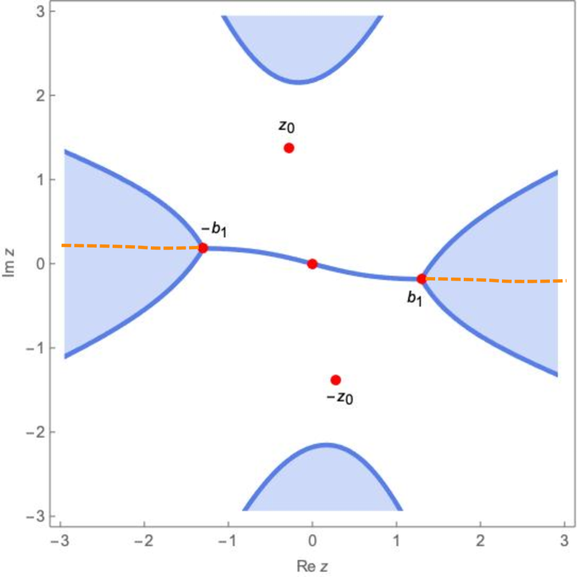
(a) $t=1+{\mathrm{i}}\in\mathcal{O}_{1}$.

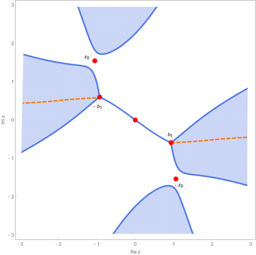
(b) $t=1+3.8{\mathrm{i}}\in\mathcal{O}_{1}$.

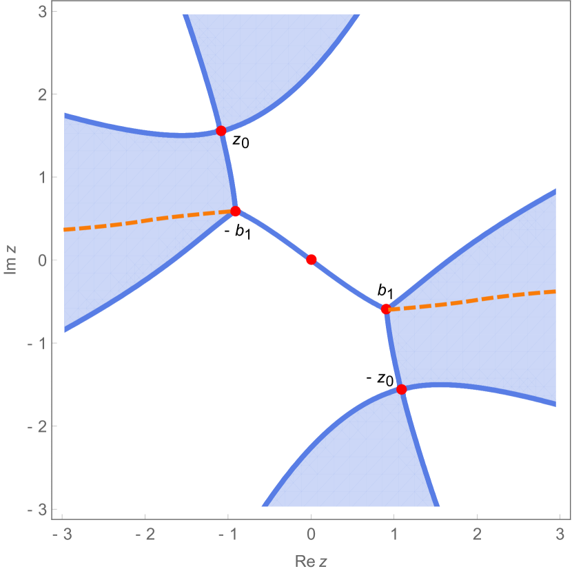
(c) $t=1+3.92{\mathrm{i}}\in\mathcal{O}_{1}$.

(d) $t=1+4{\mathrm{i}}\in\mathcal{O}_{1}$.

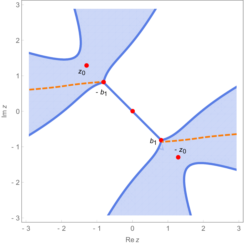
(e) $t=4{\mathrm{i}}\in\mathcal{O}_{1}$.

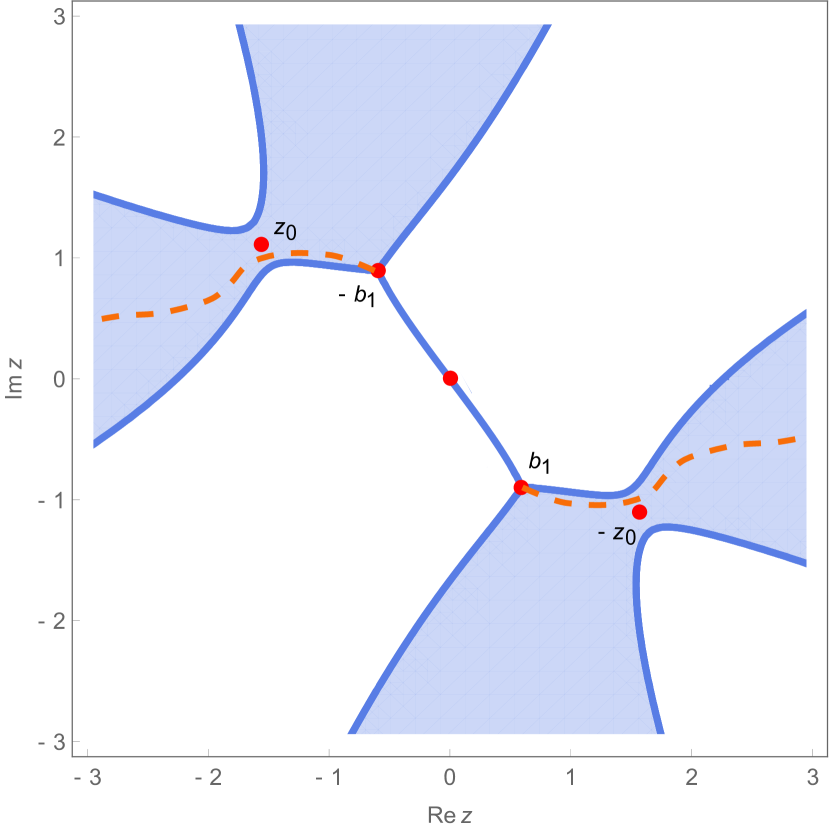
(f) $t=-1+4{\mathrm{i}}\in\mathcal{O}_{1}$.

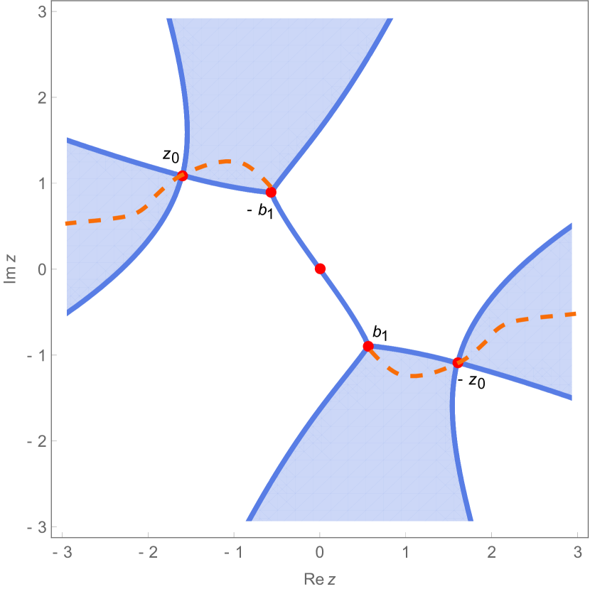
(g) $t_{\mbox{cr}}\in\gamma_{3}$.

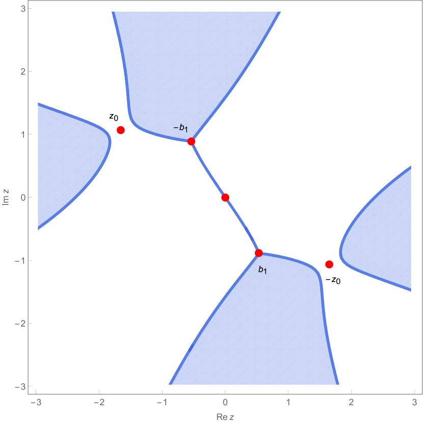
(h) $t=-1.35+4{\mathrm{i}}\notin\mathcal{O}_{1}$.

Figure 3. This sequence of figures shows allowable regions in light blue through which the contour of integration (for the orthogonal polynomials) must pass, for a varying collection of values of $t$. Regions in light blue are the $t$-stable lands where $\mathcal{U}(z;t)<0$ and the regions in white are the $t$-unstable lands where $\mathcal{U}(z;t)>0$. Figures courtesy of Roozbeh Gharakhloo.

Theorem 4.6 ([BGM]).

Let $\mu_{t}$ and $Q(z;t)$ be as in Theorem 4.4. If $t\in\overline{\mathcal{O}_{1}}$, then

(4.9) $$Q(z;t)=\dfrac{1}{4}(z^{2}-z^{2}_{0}(t))^{2}(z^{2}-b_{1}^{2}(t)),$$

where

(4.10) $$b_{1}(t)=\sqrt{\dfrac{2}{3}\left(-t+\sqrt{12+t^{2}}\right)}\quad\text{and}\quad z_{0}(t)=\sqrt{\dfrac{1}{3}\left(-2t-\sqrt{12+t^{2}}\right)},$$

with branches chosen so that for $t>-2$,

$$z_{0}(t)={\mathrm{i}}y_{0},\quad y_{0}>0\quad\text{and}\quad a_{1}(t)>0.$$

Furthermore,

1. if $t\in\mathcal{O}_{1}$, then $J_{t}=\Gamma[-b_{1},b_{1}]$ and we take $\Gamma_{t}=\Gamma({\mathrm{e}}^{{\mathrm{i}}\pi}\infty,-b_{1})\cup J_{t}\cup\Gamma(b_{1},{\mathrm{e}}^{0\pi{\mathrm{i}}}\infty),$ see Figure 3(A-D),

2. if $t\in\gamma_{j},\ j\in\{3,4\}$, then $J_{t}=\Gamma[-a_{1},a_{1}]$ and $\Gamma_{t}=\Gamma({\mathrm{e}}^{\pi{\mathrm{i}}}\infty,(-1)^{j+1}z_{0})\cup\Gamma[(-1)^{j+1}z_{0},-b_{1}]\cup J_{t}\cup\Gamma[-b_{1},(-1)^{j}z_{0}]\cup\Gamma((-1)^{j}z_{0},{\mathrm{e}}^{0\pi{\mathrm{i}}}\infty)$, see Figure 3(G),

3. if $t\in\gamma_{j},\ j\in\{1,2\}$, then the support of $\mu_{t}$ “splits” and

   $$J_{t}=\Gamma[-b_{1},(-1)^{j+1}z_{0}]\cup\Gamma[(-1)^{j+1}z_{0},(-1)^{j}z_{0}]\cup\Gamma[(-1)^{j}z_{0},b_{1}],$$

   and we choose $\Gamma_{t}=\Gamma({\mathrm{e}}^{\pi{\mathrm{i}}}\infty,-b_{1})\cup J_{t}\cup\Gamma(b_{1},{\mathrm{e}}^{0\pi{\mathrm{i}}}\infty)$, see Figure 4

4. if $t=\pm{\mathrm{i}}\sqrt{12}$, then $\pm z_{0}=\mp a_{1}$ and $J_{t}=[-b_{1},b_{1}]$ and $\Gamma_{t}$ can be chosen as in (a),

5. if $t=-2,$ then $z_{0}=0$ and the support of $\mu_{t}$ “splits into $J_{t}=\Gamma[-b_{1},0]\cup\Gamma[0,b_{1}]$, see [BGM]*Figure 6. Here, we choose $\Gamma_{t}$ as in (c).

(a) $t=-1\in\mathcal{O}_{1}$.

(b) $t=-1+{\mathrm{i}}in\mathcal{O}_{1}$.

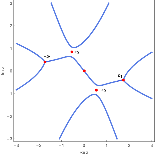
(c) $t=-1+1.6{\mathrm{i}}\in\mathcal{O}_{1}$.

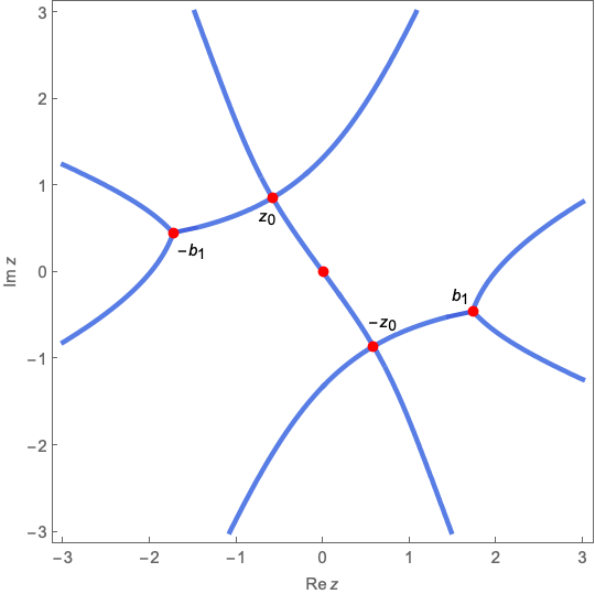
(d) $t=-1+1.78{\mathrm{i}}\notin\mathcal{O}_{1}$.

Figure 4. Same as Figure 3, except wihtout the shading. Figures courtesy of Roozbeh Gharakhloo.

To state an analogous theorem for $t\in\mathcal{O}_{2}$, we will need the following bit of notation. Let $I_{t}$ be an analytic arc connecting $-a_{2}(t),a_{2}(t)$ in such a way that it avoids the origin, lies entirely in the region $\{\mathcal{U}(z;t)<0\}$, and for a fixed neighborhood $U_{\pm a_{2}}$ of $\pm a_{2}(t)$, $I_{t}\cap U_{\pm a_{2}}$ coincides with orthogonal trajectories emanating from $\pm a_{2}$.The following theorem summarizes the relevant results from [BGM]*Section 2.4.2.

Theorem 4.7 ([BGM]).

Let $\mu_{t}$ and $Q(z;t)$ be as in Theorem 4.4. If $t\in\overline{\mathcal{O}_{2}}$, then

(4.11) $$Q(z;t)=\dfrac{1}{4}z^{2}(z^{2}-a_{2}^{2}(t))(z^{2}-b_{2}^{2}(t)),$$

where

(4.12) $$a_{2}(t)=\sqrt{-2-t},\quad b_{2}(t)=\sqrt{2-t},$$

and $\sqrt{\diamond}$ is the principle branch. Furthermore, we have that the support of $\mu_{t}$ is given by

(4.13) $$J_{t}=\Gamma[-b_{2},-a_{2}]\cup\Gamma[a_{2},b_{2}]\mathrel{\mathop{\mathchar 58\relax}}=J_{t,1}\cup J_{t,2},$$

where $J_{t,1}=\Gamma[-b_{2},-a_{2}]$ and $J_{t,2}=\Gamma[a_{2},b_{2}]$. Furthermore, we have

1. if $t\in\mathcal{O}_{2}$, then we take $\Gamma_{t}=\Gamma({\mathrm{e}}^{\pi{\mathrm{i}}}\infty,-b_{2})\cup J_{t,1}\cup I_{t}\cup J_{t,2}\cup\Gamma(b_{2},{\mathrm{e}}^{0\pi{\mathrm{i}}}\infty)$, see Figure 5(a),

2. if $t\in\gamma_{5}\cup\gamma_{6}$, then we take $\Gamma_{t}=\Gamma({\mathrm{e}}^{\pi{\mathrm{i}}}\infty,-b_{2})\cup J_{t,1}\cup I_{t}\cup J_{2,t}\cup\Gamma(b_{2},{\mathrm{e}}^{0\pi{\mathrm{i}}}\infty)$, see Figure 5(b).

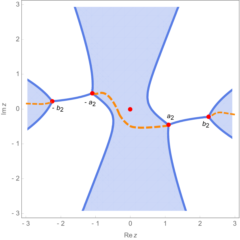
(a) $t=-3+{\mathrm{i}}\in\mathcal{O}_{2}$.

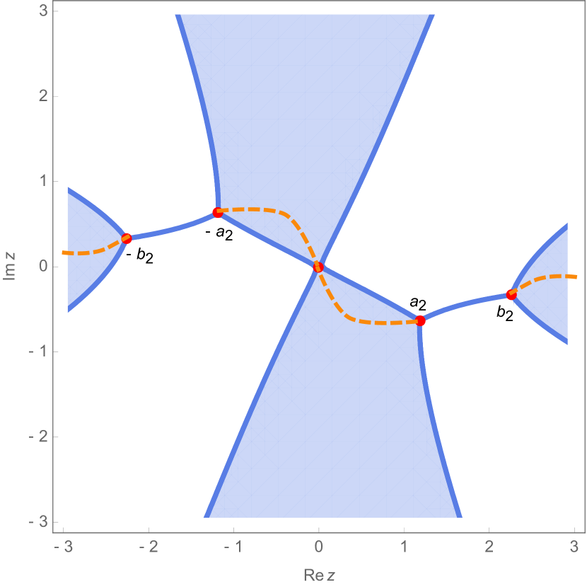
(b) $t=-3+1.5{\mathrm{i}}\in\mathcal{O}_{2}$.

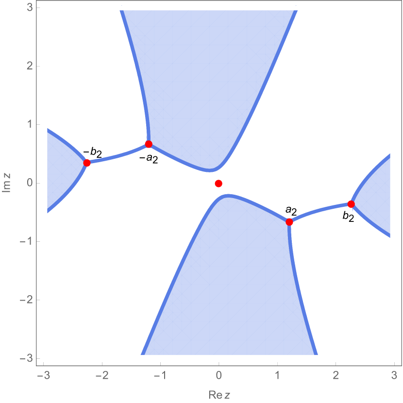
(c) $t=-3+1.6{\mathrm{i}}\not\in\mathcal{O}_{2}$.

Figure 5. Same as in Figure 3. Figures courtesy of Roozbeh Gharakhloo.

Finally, when $t\in\mathcal{O}_{3}$, $Q(z;t)$ has 6 distinct roots. These are determined by a combination of algebraic “moment conditions” as well as two integral equations. Since $t\in\mathcal{O}_{3}$ is outside of the scope of this work, we simply refer to [BGM, BBGMT]. Since we will be primarily interested in $t\in\mathcal{O}_{2}$, we record in the following remark a more explicit description of it.

Remark 4.8.

It was shown in [BGM]*Section 4.2 that the arcs $\gamma_{5},\gamma_{6}$ shown in Figure 2 are exactly the two unbounded trajectories in the left half plane of the quadratic differential

$$\frac{1}{4}(z^{2}+4)({\mathrm{d}}z)^{2}.$$

These trajectories are asymptotic to lines at angles $\pm 3\pi/4$. This is equivalent to (see [BGM]*Section 4.2 for details) the zero-set of the real part of

$$\Phi(z)\mathrel{\mathop{\mathchar 58\relax}}=\frac{1}{2}\int_{2}^{z}\sqrt{z^{2}-4}\ {\mathrm{d}}z.$$

A moment’s thought with this expression reveals that $\mathcal{O}_{2}\subseteq\{z\ \mathrel{\mathop{\mathchar 58\relax}}\ 3\pi/4<\text{arg}(z)<5\pi/4\}$.

4.3. Construction of the $g$-function

The first step in Section 5.1 will be to normalize the initial Riemann-Hilbert problem RHP-${\mathbf{Y}_{n}}$ at $z=\infty$, for which we require a function $g(z)$, colloquially known as the $g$-function:

(4.14) $$g(z;t)\mathrel{\mathop{\mathchar 58\relax}}=\int_{J_{t}}\log(z-x){\mathrm{d}}\mu_{t}(x),$$

where, for a fixed $x\in J$, we take the branch cut of $\log(z-s)$ along $\Gamma_{t}$. It follows from the definition of $g$ that

(4.15) $$U^{\mu_{t}}(z)=-\Re(g(z;t))$$

and we can now rewrite the Euler-Lagrange conditions:

(4.16) $$-\Re g(z;t)+\dfrac{1}{2}\Re V(z;t)=\left\{\begin{array}[]{ll}=\ell_{t},&z\in J_{t},\\ \geq\ell_{t},&z\in\Gamma_{t}\setminus J_{t}.\end{array}\right.$$

Furthermore, we note that

(4.17) $$g^{\prime}(z;t)=\int_{J_{t}}\dfrac{{\mathrm{d}}\mu_{t}(x)}{z-x}.$$

The $g$ function was constructed in [BGM], and we summarize its relevant features here. In particular, we focus our attention on $t\in\mathcal{O}_{2}\cup\mathcal{O}_{3}$, since $t\in\mathcal{O}_{1}$ was already analyzed in [BGM].

4.3.1. Two-cut case.

Combining (4.6),(4.11), and (4.17), we conclude that there exists a constant $\ell^{(2)}_{*}(t)$ such that

(4.18) $$g(z;t)=\dfrac{V(z;t)+\ell_{*}^{(2)}(t)+\eta_{2}(z;t)}{2},\quad z\in{\mathbb{C}}\setminus\Gamma_{t}(-\infty,b_{2}],$$

where

(4.19) $$\eta_{2}(z;t)\mathrel{\mathop{\mathchar 58\relax}}=-2\int_{b_{2}}^{z}Q^{1/2}(x;t){\mathrm{d}}x,$$

where the path of integration is taken to be in ${\mathbb{C}}\setminus\Gamma_{t}(-\infty,b_{2}]$. It will be convenient to introduce the following notation: for $e\in\{\pm a_{2},\pm b_{2}\}$, let

(4.20) $$\eta_{2,e}(z)\mathrel{\mathop{\mathchar 58\relax}}=-2\int_{e}^{z}Q^{1/2}(x){\mathrm{d}}x,\quad$$

where the path of integration is taken in

• ${\mathbb{C}}\setminus\Gamma_{t}(-\infty,b_{2}]$ when $e=b_{2}$,

• ${\mathbb{C}}\setminus\Gamma_{t}[-b_{2},\infty)$ when $e=-b_{2}$,

• ${\mathbb{C}}\setminus\Gamma_{t}(-\infty,-a_{2}]\cup\Gamma[a_{2},\infty)$ when $e\in\{\pm a_{2}\}$.

Then, it follows from definition (4.19) that $\eta_{2}(z)=\eta_{2,b_{2}}(z)$. Note that since $\mu_{t}$ in (4.7) is a probability measure, and using the evenness of $Q^{1/2}_{+}$, we have

$$\dfrac{1}{\pi{\mathrm{i}}}\int_{J_{t,1}}Q^{1/2}_{+}(x){\mathrm{d}}x=\dfrac{1}{\pi{\mathrm{i}}}\int_{J_{t,2}}Q^{1/2}_{+}(x){\mathrm{d}}x=\dfrac{1}{2}.$$

Using this, we can deduce that

(4.21) $$\eta_{2,b_{2}}(z;t)=\left\{\begin{array}[]{l}\eta_{2,a_{2}}(z;t)\pm\pi{\mathrm{i}},\\ \eta_{2,-a_{2}}(z;t)\pm\pi{\mathrm{i}},\\ \eta_{2,-b_{2}}(z;t)\pm 2\pi{\mathrm{i}}\end{array}\right.\quad z\in{\mathbb{C}}\setminus\Gamma,$$

where the plus/minus signs correspond to $z$ on the left/right of $\Gamma_{t}$, respectively.

It turns out, $\eta_{2}$ (and consequently, all $\eta_{2,e}$) can be written in terms of elementary functions. Specifically, note that one can rewrite

(4.22) $$Q^{1/2}(z;t)=\dfrac{1}{2}zR^{1/2}(z;t)$$

where $R^{1/2}(z;t)=\sqrt{(z^{2}-a_{2}^{2})(z^{2}-b_{2}^{2})}$ is the branch of the square root analytic in ${\mathbb{C}}\setminus J_{t}$ and satisfies $R^{1/2}(z)=z^{2}+O(z)$ as $z\to\infty$, then one can check that

(4.23) $$\eta_{2}(z;t)=-\dfrac{1}{4}(z^{2}+t)R^{1/2}(z)+\log\left(\dfrac{2z^{2}+t+R^{1/2}(z)}{2}\right),\quad z\in{\mathbb{C}}\setminus\Gamma_{t}(-\infty,b_{2}].$$

Then, using (4.18), the $g$ functions can be written explicitly

(4.24) $$g(z;t)=\dfrac{1}{2}\left(\dfrac{tz^{2}}{2}+\dfrac{z^{4}}{4}+\ell_{*}^{(2)}(t)\right)-\dfrac{1}{8}(z^{2}+t)R^{1/2}(z)+\dfrac{1}{2}\log\left(\dfrac{2z^{2}+t+R^{1/2}(z)}{2}\right).$$

Combining this expression with the requirement that

(4.25) $$g(z;t)=\log z+O(z^{-1})$$

yields

(4.26) $$\ell_{*}^{(2)}(t)=\dfrac{t^{2}}{4}-\dfrac{1}{2}.$$

Furthermore, $g(z;t)$ has the following jumps

(4.27) $$(g_{+}-g_{-})(z;t)=\left\{\begin{array}[]{ll}0,&z\in\Gamma[b_{2},\infty),\\ \eta_{2,+}(z;t),&z\in\Gamma[a_{2},b_{2}],\\ \pi{\mathrm{i}},&z\in\Gamma[-a_{2},a_{2}],\\ \eta_{2,+}(z;t),&z\in\Gamma[-b_{2},-a_{2}],\\ 2\pi{\mathrm{i}},&z\in\Gamma(-\infty,-b_{2}],\end{array}\right.$$

and

(4.28) $$\left(g_{+}+g_{-}-V-\ell_{*}^{(2)}\right)(z;t)=\left\{\begin{array}[]{ll}\eta_{2}(z;t),&z\in\Gamma[b_{2},\infty),\\ 0,&z\in\Gamma[a_{2},b_{2}],\\ \eta_{2,\pm}(z;t)\mp\pi{\mathrm{i}},&z\in\Gamma[-a_{2},a_{2}],\\ 0,&z\in\Gamma[-b_{2},-a_{2}],\\ \eta_{2,\pm}(z;t)\mp 2\pi{\mathrm{i}},&z\in\Gamma(-\infty,-b_{2}],\end{array}\right.$$

where the second-to-last line in both formulas uses the fact that

$$\int_{-a_{2}}^{a_{2}}x\sqrt{(x^{2}-a_{2}^{2})(x^{2}-b_{2}^{2})}{\mathrm{d}}x=0.$$

The arcs $\Gamma[a_{2},b_{2}]\cup\Gamma[-b_{2},-a_{2}]$ are solutions of $\Re[\eta_{2}(z;t)]=0$; in fact, it was shown in [BGM]*Section 3.2 that for all $t\in\mathcal{O}_{2}$, there exists a (non-unique) choice of $\Gamma_{t}$ so that

(4.29) $$\Re[\eta_{2}(z;t)]<0,\quad z\in\Gamma_{t}\setminus J_{t}.$$

Furthermore, it follows from (4.8), (4.15) , and the subharmonicity of $\mathcal{U}$ that $\Re[\eta_{2}(z;t)]$ is subharmonic of any point $z_{0}\in J_{t}$. We then deduce from the maximum principle for subharmonic functions that every $z\in J_{t,1}\cup J_{t,2}$ is on the boundary of the set $\Re[\eta_{2}(z;t)]>0$. See Figure 5.

4.4. Szegő function

To handle the general double-scaling limit where $\{N_{n}\}_{n=1}^{\infty}\subseteq{\mathbb{N}}$ with $|N_{n}-n|<C$ for a fixed $C\geq 0$, we will need the Szegő function of ${\mathrm{e}}^{V(z;t)}$. The following proposition defines and summarizes its properties.

Proposition 4.9.

Let $R^{1/2}(z;t)$ be is as in (4.22). Then, the Szegő function

(4.30) $$\mathcal{D}(z;t)\mathrel{\mathop{\mathchar 58\relax}}=\exp\left(\dfrac{1}{2}V(z;t)-\dfrac{1}{8}(z^{2}+t)R^{1/2}(z;t)\right).$$

is analytic in $\overline{{\mathbb{C}}}\setminus J_{t}$ and has continuous traces on $J_{t}\setminus\{\pm a_{2},\pm b_{2}\}$ which satisfy

(4.31) $$\mathcal{D}_{+}(x;t)\mathcal{D}_{-}(x;t)={\mathrm{e}}^{V(x;t)},\quad x\in J_{t}.$$

Furthermore, $\mathcal{D}(z;t)$ is bounded as $z\to e\in\{\pm a_{2},\pm b_{2}\}$, and

(4.32) $$\mathcal{D}(z;t)={\mathrm{e}}^{-\ell_{*}^{(2)}(t)/2}\left(1+\dfrac{1}{4z^{4}}+\mathcal{O}\left(\dfrac{1}{z^{6}}\right)\right)\quad\text{as}\quad z\to\infty,$$

where $\ell_{*}^{(2)}(t)$ is as in (4.26).

Remark 4.10.

Henceforth, we let $D(z;t)\mathrel{\mathop{\mathchar 58\relax}}={\mathrm{e}}^{\ell_{*}^{(2)}(t)/2}\mathcal{D}(z;t)$ be the normalized Szegő function.

Proof.

From (4.22) it follows that $R^{1/2}(z;t)$ is analytic in ${\mathbb{C}}\setminus J_{t}$ and for $z\in J_{t}\setminus\{\pm a_{2},\pm b_{2}\}$ we have $R^{1/2}(z;t)_{+}=-R^{1/2}(z;t)_{-}$. This implies (4.31). At $z=\infty$, we note that by (4.6) and the choice if the square root, we have

(4.33) $$Q^{1/2}(z,t)=\dfrac{V^{\prime}(z,t)}{2}-\dfrac{1}{z}+\mathcal{O}\left(\dfrac{1}{z^{3}}\right)\quad\text{as}\quad z\to\infty.$$

By definition of $R^{1/2}$ and (4.33) we find

(4.34) $$(z^{2}+t)R^{1/2}(z;t)=4V(z;t)+4\ell^{(2)}_{*}(t)+\mathcal{O}\left(\frac{1}{z^{2}}\right)\quad\text{as}\quad z\to\infty.$$

Hence, $\mathcal{D}(z;t)$ has a convergent Laurent expansion centered at $z=\infty$ of the form (4.32). ∎

4.5. Riemann surface

We will need an arsenal of functions that naturally live on an associated Riemann surface, which we introduce here. Let $R(z;t)=(z^{2}-a_{2}^{2}(t))(z^{2}-b_{2}^{2}(t))$ and

$$\mathfrak{S}\mathrel{\mathop{\mathchar 58\relax}}=\left\{(z,w)\ \mathrel{\mathop{\mathchar 58\relax}}\ w^{2}=R(z)\right\}.$$

Denote by $\pi\mathrel{\mathop{\mathchar 58\relax}}\mathfrak{S}\to\overline{\mathbb{C}}$ the natural projection $\pi({\boldsymbol{z}})=z$ and by $\diamond^{*}\mathrel{\mathop{\mathchar 58\relax}}\mathfrak{S}\to\mathfrak{S}$ the natural involution ${\boldsymbol{z}}=(z,w)\implies{\boldsymbol{z}}^{*}=(z,w)^{*}=(z,-w)$. We use notation ${\boldsymbol{z}},{\boldsymbol{x}},\boldsymbol{a}$ for points on $\mathfrak{S}$ with natural projections $z,x,a$.

The function $w({\boldsymbol{z}})$, defined by $w^{2}({\boldsymbol{z}})=R(z)$, is meromorphic on $\mathfrak{S}$ with simple zeros at the ramification points $\boldsymbol{E}_{t}=\{\pm\boldsymbol{a}_{2},\pm\boldsymbol{b}_{2}\}$, double poles at the points on top of infinity, and is otherwise non-vanishing and finite. Put

$$\boldsymbol{\Delta}\mathrel{\mathop{\mathchar 58\relax}}=\pi^{-1}(J_{t})\quad\text{and}\quad\mathfrak{S}=\mathfrak{S}^{(0)}\cup\boldsymbol{\Delta}\cup\mathfrak{S}^{(1)},$$

where the domains $\mathfrak{S}^{(k)}$ project onto $\overline{\mathbb{C}}\setminus J_{t}$ with labels chosen so that $w({\boldsymbol{z}})=(-1)^{k}z^{2}+O(z)$ as ${\boldsymbol{z}}$ approaches the point on top of infinity within $\mathfrak{S}^{(k)}$. For $z\in\overline{\mathbb{C}}\setminus J_{t}$ we let $z^{(k)}$ stand for the unique ${\boldsymbol{z}}\in\mathfrak{S}^{(k)}$ with $\pi({\boldsymbol{z}})=z$. We define a homology basis on $\mathfrak{S}$ in the following way: we let (see discussion before Theorem 4.7)

$$\boldsymbol{\alpha}\mathrel{\mathop{\mathchar 58\relax}}=\pi^{-1}(I_{t})\quad\text{and}\quad\boldsymbol{\beta}\mathrel{\mathop{\mathchar 58\relax}}=\pi^{-1}(J_{t,1}),$$

where $\boldsymbol{\alpha}$ is oriented towards $-\boldsymbol{a}_{2}$ within $\mathfrak{S}^{(0)}$ and $\boldsymbol{\beta}$ is oriented so that $\boldsymbol{\alpha},\boldsymbol{\beta}$ form the right pair at $-\boldsymbol{a}_{2}$, see Figure 6. We will often use the notation $\mathfrak{S}_{{\boldsymbol{\alpha}},{\boldsymbol{\beta}}}\mathrel{\mathop{\mathchar 58\relax}}=\mathfrak{S}\setminus\{{\boldsymbol{\alpha}},{\boldsymbol{\beta}}\}$.

Figure 6. Schematic representation of the surface $\mathfrak{S}$ (shaded region represents $\mathfrak{S}^{(1)}$), which topologically is a torus, and the homology basis $\boldsymbol{\alpha},\boldsymbol{\beta}$ .

Surface $\mathfrak{S}$ is genus 1, and so the vector space of holomorphic differentials is one dimensional and we choose the following basis

(4.35) $$\mathcal{H}(z)=\left(\int_{\boldsymbol{\alpha}}\dfrac{{\mathrm{d}}x}{w({\boldsymbol{x}})}\right)^{-1}\dfrac{{\mathrm{d}}z}{w({\boldsymbol{z}})},$$

which is normalized to have period 1 on $\boldsymbol{\alpha}$; it follows by classical theory (see, e.g. [MR583745]) that when $t\in\mathcal{O}_{2}$,

$$\mathrm{B}(t)\mathrel{\mathop{\mathchar 58\relax}}=\int_{\boldsymbol{\beta}}\mathcal{H}\implies\Im\mathrm{B}(t)>0.$$

In what follows, we suppress the dependence of ${\mathrm{B}}(t)$ on $t$ and write ${\mathrm{B}}(t)={\mathrm{B}}$.

4.5.1. Abel’s map

Let ${\mathcal{A}}\mathrel{\mathop{\mathchar 58\relax}}\mathfrak{S}_{{\boldsymbol{\alpha}},{\boldsymbol{\beta}}}\to{\mathbb{C}}$ be the abelian integral

(4.36) $$\mathcal{A}({\boldsymbol{z}})\mathrel{\mathop{\mathchar 58\relax}}=\int_{{\boldsymbol{b}}_{2}}^{\boldsymbol{z}}\mathcal{H},\quad{\boldsymbol{z}}\in\mathfrak{S}_{{\boldsymbol{\alpha}},{\boldsymbol{\beta}}},$$

where the path of integration is taken in $\mathfrak{S}_{{\boldsymbol{\alpha}},{\boldsymbol{\beta}}}$. ${\mathcal{A}}$ is holomorphic in $\mathfrak{S}_{{\boldsymbol{\alpha}},{\boldsymbol{\beta}}}$, and it follows from the definition of ${\mathrm{B}}$ and the normalization of $\mathcal{H}$ that

(4.37) $$({\mathcal{A}}_{+}-{\mathcal{A}}_{-})({\boldsymbol{x}})=\left\{\begin{array}[]{rl}-{\mathrm{B}},&{\boldsymbol{x}}\in{\boldsymbol{\alpha}}\setminus\{-{\boldsymbol{a}}_{2}\},\vskip 6.0pt plus 2.0pt minus 2.0pt\\ 1,&{\boldsymbol{x}}\in{\boldsymbol{\beta}}\setminus\{-{\boldsymbol{a}}_{2}\}.\end{array}\right.$$

Let ${\mathrm{Jac}}(\mathfrak{S})={\mathbb{C}}/\{{\mathbb{Z}}+{\mathrm{B}}{\mathbb{Z}}\}$ denote the Jacobi variety of $\mathfrak{S}$, whose elements are the following equivalence classes, given $x\in{\mathbb{C}}$,

$$[x]=\{x+k+j{\mathrm{B}}\in{\mathbb{C}}\ \mathrel{\mathop{\mathchar 58\relax}}x\in\ k,j\in{\mathbb{Z}}\}.$$

It follows from (4.37) that the Abel’s map ${\boldsymbol{z}}\mapsto[{\mathcal{A}}({\boldsymbol{z}})]$ is well-defined. In fact, since $\mathfrak{S}$ has genus 1, it is an isomorphism [MR583745]*Section III.6. We will use this to formulate a Jacobi inversion problem in Section 4.6.

4.6. Jacobi inversion problem

In view of the Abel map being an isomorphism, let ${\boldsymbol{z}}_{[x]}$ denote the unique solution to the equation

$$\left[{\mathcal{A}}\left({\boldsymbol{z}}_{[x]}\right)\right]=[x].$$

The problem of determining ${\boldsymbol{z}}_{[x]}$ for a given $x\in{\mathbb{C}}$ is known as the Jacobi inversion problem. We will be interested in two problems, namely

(4.38) $$\left[{\mathcal{A}}\left({\boldsymbol{z}}_{k,[x_{*}]}\right)\right]=[x_{*}]\quad\text{ where }\quad x_{*}={\mathcal{A}}\left(0^{(k)}\right)+\dfrac{1}{2},\quad k\in\{0,1\}.$$

Due to various symmetries of $\mathfrak{S}$, it turns out we can solve this problem exactly. This is the content of the following proposition.

Proposition 4.11.

Let $x_{*}$ be as above, and $k\in\{0,1\}$ then ${\boldsymbol{z}}_{k,[x_{*}]}=0^{(1-k)}$.

Proof.

Let $\tilde{{\boldsymbol{\alpha}}}$ be an involution-symmetric cycle homologous to ${\boldsymbol{\alpha}}$ containing $0^{(0)},0^{(1)}$, and note the following two symmetries:

(4.39) $$\int_{\pm\boldsymbol{a}_{2}}^{{\boldsymbol{z}}}\mathcal{H}=-\int_{\pm\boldsymbol{a}_{2}}^{{\boldsymbol{z}}^{*}}\mathcal{H},\quad\text{and}\quad\int_{\pm\boldsymbol{a}_{2}}^{0^{(k)}}\mathcal{H}=\int_{0^{(k)}}^{\mp\boldsymbol{a}_{2}}\mathcal{H}.$$

Indeed, the first equality follows from $w({\boldsymbol{z}}^{*})=-w({\boldsymbol{z}}^{*})$ while the other follows from $w(\pi({\boldsymbol{z}}))=w(-\pi({\boldsymbol{z}}))$. Using the first symmetry and normalization (4.35), for a path contained in $\mathfrak{S}^{(1)}$ we have that

$$\int_{-\boldsymbol{a}_{2}}^{\boldsymbol{a}_{2}}\mathcal{H}=\dfrac{1}{2}.$$

Using this and the above symmetries, we have

$$\dfrac{1}{2}=\int_{-\boldsymbol{a}_{2}}^{\boldsymbol{a}_{2}}\mathcal{H}=\int_{-\boldsymbol{a}_{2}}^{0^{(1)}}\mathcal{H}+\int_{0^{(1)}}^{\boldsymbol{a}_{2}}\mathcal{H}=-\int_{-\boldsymbol{a}_{2}}^{0^{(0)}}\mathcal{H}+\int_{0^{(1)}}^{\boldsymbol{a}_{2}}\mathcal{H}\\ =\int_{0^{(0)}}^{-\boldsymbol{a}_{2}}\mathcal{H}+\int_{0^{(1)}}^{\boldsymbol{a}_{2}}\mathcal{H}=\int^{0^{(0)}}_{\boldsymbol{a}_{2}}\mathcal{H}+\int_{0^{(1)}}^{\boldsymbol{a}_{2}}\mathcal{H}.$$

So, $\left[{\mathcal{A}}\left(0^{(0)}\right)-{\mathcal{A}}\left(0^{(1)}\right)\right]=\left[1/{2}\right]$. Noting that $[1/2]=[-1/2]$ yields the desired result. ∎

In fact, the proof of the above proposition yields a slightly better identity, namely that

$${\mathcal{A}}(0^{(0)})={\mathcal{A}}(0^{(1)})+\dfrac{1}{2},$$

which we will use in the following subsection.

4.7. Theta functions

Let $\theta(x;{\mathrm{B}})$ be the Riemann theta function associated with ${\mathrm{B}}$, i.e.,

(4.40) $$\theta(x;{\mathrm{B}})=\sum_{k\in{\mathbb{Z}}}\exp\left(\pi{\mathrm{i}}\mathsf{{\mathrm{B}}}k^{2}+2\pi{\mathrm{i}}xk\right),\quad x\in{\mathbb{C}}.$$

The function $\theta(x)$ is holomorphic in ${\mathbb{C}}$ and enjoys the following periodicity properties:

(4.41) $$\theta(x+j+{\mathrm{B}}m)=\exp\left\{-\pi{\mathrm{i}}{\mathrm{B}}m^{2}-2\pi{\mathrm{i}}xm\right\}\theta(x),\qquad j,m\in{\mathbb{Z}}.$$

It is also known that $\theta(x)$ vanishes only at the points of the lattice $\left[\frac{\mathsf{B}+1}{2}\right]$. Let

(4.42) $$\Theta({\boldsymbol{z}})=\frac{\theta\left({\mathcal{A}}({\boldsymbol{z}})-{{\mathcal{A}}}\left(0^{(1)}\right)-\frac{\mathsf{B}+1}{2}\right)}{\theta\left({\mathcal{A}}({\boldsymbol{z}})-{{\mathcal{A}}}\left(0^{(0)}\right)-\frac{\mathsf{B}+1}{2}\right)}.$$

The functions $\Theta({\boldsymbol{z}})$ are meromorphic on $\mathfrak{S}\setminus\boldsymbol{\alpha}$ with exactly one simple pole at ${\boldsymbol{z}}=0^{(0)}$, and exactly one simple zero at ${\boldsymbol{z}}=0^{(1)}$ ($\Theta$ can be analytically continued to multiplicatively multi-valued functions on the whole surface $\mathfrak{S}$; thus, we can talk about simplicity of a pole or zero whether it belongs to the cycles of a homology basis or not). Moreover, according to (4.37), (4.40), and (4.42), they possess continuous traces on $\boldsymbol{\alpha},\boldsymbol{\beta}$ away from $-\boldsymbol{a}_{2}$ that satisfy

(4.43) $$\Theta_{+}({\boldsymbol{x}})={\mathrm{e}}^{\pi{\mathrm{i}}}\Theta_{-}({\boldsymbol{x}}),\quad{\boldsymbol{x}}\in{\boldsymbol{\alpha}}\setminus\{-\boldsymbol{a}_{2}\}.$$

4.8. More auxiliary functions

Let

(4.44) $$\gamma(z)\mathrel{\mathop{\mathchar 58\relax}}=\left(\dfrac{z-b_{2}}{z+b_{2}}\dfrac{z+a_{2}}{z-a_{2}}\right)^{1/4},\quad z\in\overline{{\mathbb{C}}}\setminus J_{t},$$

be the branch analytic outside of $J_{t}$ and satisfying $\gamma(\infty)=1$. Furthermore, let

(4.45) $$A(z)\mathrel{\mathop{\mathchar 58\relax}}=\dfrac{\gamma(z)+\gamma^{-1}(z)}{2},\quad B(z)\mathrel{\mathop{\mathchar 58\relax}}=\dfrac{\gamma(z)-\gamma^{-1}(z)}{2{\mathrm{i}}},\quad z\in\overline{{\mathbb{C}}}\setminus J_{t}.$$

Both $A(z),B(z)$ are analytic in $\overline{{\mathbb{C}}}\setminus J_{t}$ and satisfy

(4.46) $$A(\infty)=1,\quad\text{and}\quad B(\infty)=0.$$

Furthermore, they satisfy

(4.47) $$A_{+}(x)=B_{-}(x)\quad\text{and}\quad A_{-}(x)=-B_{+}(x),\quad x\in J_{t}\setminus\{\pm a_{2},\pm b_{2}\}.$$

Observe that with the choice of branch of $\gamma$, we have that $B(0)=0$. Indeed, the equation $(AB)(z)=0$ is equivalent to $\gamma^{4}(z)=1$, which has two solutions in $\overline{{\mathbb{C}}}$, namely $z=\infty$ and $z=0$. To see that $z=0$ is a root of $B(z)$ instead of $A(z)$, we’ll show that $\gamma(0)=1$. To this end, let $w=\gamma^{4}(z)$ and observe that $\gamma^{4}(J_{t,1})$ is a contour connecting $w=0$ to $w=\infty$. Observe that

$$\gamma^{4}(z)=\gamma^{4}(x)\implies z=x\quad\text{or}\quad z=-\dfrac{a_{2}b_{2}}{x}.$$

Let $L$ denote a contour connecting $z=\infty$ to $z=0$ while avoiding $J_{t,1}$ and its image under the map $z\mapsto-a_{2}b_{2}/z$. Then, $\gamma^{4}(L)$ is a closed contour containing $w=1$ and not winding around the origin. Hence, the continuation of the principle branch of $\diamond^{1/4}$ along $\gamma^{4}(L)$ is single-valued, and produces $\gamma(L)$. Finally, since $\gamma(\infty)=1$, we have $\gamma(0)=1$ as desired.

4.9. Statement of asymptotic results

To formulate the following theorem requires the following definition (cf. [MR3607591]*Definition 4.2).

Definition 4.12.

An estimate $f_{n}(z,t)=\mathcal{O}(n^{-\alpha})$ holds $(z,t)$-locally uniformly for $z\in V$ as $n\to\infty$ if for each compact $T\subseteq\mathcal{O}_{2}$ and any collection of compact sets $\{K_{t}\}_{t\in K}$ such that $\cup_{t\in T}K_{t}\subseteq V$, there is a constant $C(V;T)<\infty$ such that

$$|f_{n}(z;t)|\leq C(V;T)n^{-\alpha},\quad z\in K_{t},\quad t\in T,$$

for all $N$ large enough.

We are now ready to state our main results regarding the asymptotic behavior of the orthogonal polynomials and their recurrence coefficients and normalizing constants.

Theorem 4.13.

Let $t\in\mathcal{O}_{2}$ and $\{N_{n}\}_{n\in{\mathbb{N}}}$ be a sequence of integers such that there exists $C\in{\mathbb{N}}$ with $|N_{n}-n|<C$ for all $n\in{\mathbb{N}}$. Then,

(4.48) $$P_{n}(z)={\mathrm{e}}^{ng(z)}\left(\left(D^{(N_{n}-n)}(z)A(z)\cdot\left\{\begin{array}[]{ll}1,&n\in 2{\mathbb{N}},\vskip 6.0pt plus 2.0pt minus 2.0pt\\ \dfrac{\Theta^{(0)}(\infty)}{\Theta^{(0)}(z)},&n\in{\mathbb{N}}\setminus 2{\mathbb{N}}\end{array}\right\}\right.+\mathcal{O}\left(\dfrac{1}{n}\right)\right),\quad\text{as}\quad n\to\infty,$$

$(z,t)$-locally uniformly in ${\mathbb{C}}\setminus J_{t}$.

Remark 4.14.

Note that the oddness of the function $P_{2n+1}(z;t,N)$ is reflected in the fact that the leading term in (4.48) vanishes at $z=0$ since $\Theta^{(0)}(z)$ possesses a simple pole there.

Formulas similar to (4.48) can easily be deduced in the interior of $J_{t}$, but since we do not use these we do not state them here. One immediate consequence of Theorem 4.13 and (4.25) is that for all $t\in\mathcal{O}_{2}$ and $n$ large enough, $\text{deg}P_{n}=n$. In view of the discussion in Section 3.2 we have the following corollary.

Corollary 4.15.

Let $K\subseteq\mathcal{O}_{2}$ be a compact set and $\{N_{n}\}_{n\in{\mathbb{N}}}$ be a sequence such that for all $n$. Then, there exists $n_{*}\in{\mathbb{N}}$ large enough so that for all $n>n_{*}$, $H_{n}(t,N_{n})$ is nonvanishing for $t\in K$, and $h_{n}(t,N_{n}),\gamma_{n}^{2}(t,N_{n})$ are nonvanishing and bounded for $t\in K$.

Remark 4.16.

The same boundedness and nonvanishing result is already known for $K\subseteq\mathcal{O}_{1}$; this follows directly from the asymptotic analysis in [BGM]. In fact, motivated by Figure 1, one might suspect that the results can be extended to closed subsets of $\mathcal{O}_{1},\mathcal{O}_{2}$. An analogous story takes place in the Cubic Model, where boundedness on compact subsets of the one-cut region was shown in [MR3607591] and upgraded to closed subsets in [BBDY].

The asymptotic analysis in Section 5 also yields asymptotic formulas for $\gamma_{n}^{2},h_{n}$, which are stated in the following theorem.

Theorem 4.17.

Let $t\in\mathcal{O}_{2}$, $\{N_{n}\}_{n\in{\mathbb{N}}}$ be as in Theorem 4.13, and $a_{2}(t),b_{2}(t)$ be as in (4.12). Then,

(4.49) $$\gamma^{2}_{n}(t,N_{n})=\left\{\begin{array}[]{ll}\dfrac{1}{4}(a_{2}(t)-b_{2}(t))^{2},&n\in 2{\mathbb{N}},\vskip 6.0pt plus 2.0pt minus 2.0pt\\ \dfrac{4}{(a_{2}(t)-b_{2}(t))^{2}},&n\in{\mathbb{N}}\setminus 2{\mathbb{N}}.\end{array}\right\}+\mathcal{O}\left(\dfrac{1}{n}\right)\quad\text{as}\quad n\to\infty.$$

Furthermore, with $\ell^{(2)}_{*}$ given by (4.26), we have

(4.50) $$h_{n}(t,N_{n})=2\pi{\mathrm{e}}^{N_{n}\ell_{*}^{(2)}}\left\{\begin{array}[]{ll}\dfrac{1}{2}(a_{2}(t)-b_{2}(t)),&n\in 2{\mathbb{N}},\vskip 6.0pt plus 2.0pt minus 2.0pt\\ \dfrac{2}{a_{2}(t)-b_{2}(t)},&n\in{\mathbb{N}}\setminus 2{\mathbb{N}}.\end{array}\right\}+\mathcal{O}\left(\dfrac{1}{n}\right)\quad\text{as}\quad n\to\infty.$$

Finally, for all $n\in{\mathbb{N}}$ large enough, we have

(4.51) $$\mathfrak{p}_{2n,2n-2}(t,N_{2n}) ={nt}+\dfrac{(a_{2}-b_{2})^{2}}{8}+\mathcal{O}\left(\frac{1}{n}\right)\quad\text{as}\quad n\to\infty,$$

(4.52) $$\mathfrak{p}_{2n-1,2n-3}(t,N_{2n}) ={nt}+\dfrac{3a_{2}^{2}+2a_{2}b_{2}+3b_{2}^{2}}{8}+\mathcal{O}\left(\frac{1}{n}\right)\quad\text{as}\quad n\to\infty.$$

Corollary 1.5 is an immediate consequence of Theorems 1.3 and 4.17. We end this section with a few remarks:

Remark 4.18.

We may deduce (5.33) from (4.51), (4.52), Lemma 3.3, and the identity

$$\dfrac{(a_{2}+b_{2})^{2}}{4}=\dfrac{4}{(a_{2}-b_{2})^{2}}.$$

The latter follows directly from definitions (4.12).

Remark 4.19.

A particular instance of (4.49) has already appeared in the literature; when $t\in(-\infty,-2)$, (4.49) reduces to

(4.53) $$\gamma^{2}_{n}(t,N_{n})=\left\{\begin{array}[]{ll}\dfrac{-t-\sqrt{t^{2}-4}}{2},&n\in 2{\mathbb{N}},\vskip 6.0pt plus 2.0pt minus 2.0pt\\ \dfrac{-t+\sqrt{t^{2}-4}}{2},&n\in{\mathbb{N}}\setminus 2{\mathbb{N}},\end{array}\right\}+\mathcal{O}\left(\dfrac{1}{n}\right)\quad\text{as}\quad n\to\infty,$$

which agrees with [MR1715324]*Theorem 1.1 for all $n\in{\mathbb{N}}$ large enough.

Remark 4.20.

We take a moment to point out that the leading orders in (1.31), (1.32) are consistent with (3.14), (3.15), and (1.3).

5. Riemann-Hilbert Analysis

5.1. Initial Riemann-Hilbert problem

Henceforth, we omit the dependence on $t$ whenever it does not cause ambiguity. In what follows, we will denote matrices with bold, capitalized symbols (e.g. $\mathbf{Y}$), with the exception of the Pauli matrices:

$$\mathbb{I}\mathrel{\mathop{\mathchar 58\relax}}=\begin{bmatrix}1&0\\ 0&1\end{bmatrix},\quad\sigma_{1}\mathrel{\mathop{\mathchar 58\relax}}=\begin{bmatrix}0&1\\ 1&0\end{bmatrix},\quad\sigma_{2}\mathrel{\mathop{\mathchar 58\relax}}=\begin{bmatrix}0&-{\mathrm{i}}\\ {\mathrm{i}}&0\end{bmatrix}\quad\text{and}\quad\sigma_{3}\mathrel{\mathop{\mathchar 58\relax}}=\begin{bmatrix}1&0\\ 0&-1\end{bmatrix},$$

and will use the notation

$$f^{\sigma_{3}}\mathrel{\mathop{\mathchar 58\relax}}=\begin{bmatrix}f&0\\ 0&f^{-1}\end{bmatrix}.$$

We are seeking solutions of the following sequence of Riemann-Hilbert problems for $2\times 2$ matrix functions (RHP-${\mathbf{Y}_{n}}$):

1. $\mathbf{Y}_{n}(z)$ is analytic in ${\mathbb{C}}\setminus\Gamma$ and $\lim_{{\mathbb{C}}\setminus\Gamma\ni z\to\infty}\mathbf{Y}_{n}(z)z^{-n\sigma_{3}}=\mathbf{I}$;

2. $\mathbf{Y}_{n}(z)$ has continuous traces on $\Gamma$ that satisfy

   $$\mathbf{Y}_{n,+}(x)=\mathbf{Y}_{n,-}(x)\begin{bmatrix}1&{\mathrm{e}}^{-N_{n}V(x)}\\ 0&1\end{bmatrix},$$

   where, as before, $V(z)$ is given by (1.6) and the sequence $\{N_{n}\}$ is such that $|n-N_{n}|\leq N_{*}$ for some $N_{*}>0$.

The connection of RHP-${\mathbf{Y}_{n}}$ to orthogonal polynomials was first demonstrated by Fokas, Its, and Kitaev in [FIK2] and lies in the following. If the solution of RHP-${\mathbf{Y}_{n}}$ exists, then it is necessarily of the form

(5.1) $$\mathbf{Y}_{n}(z)=\begin{bmatrix}P_{n}(z)&\big{(}\mathcal{C}P_{n}{\mathrm{e}}^{-N_{n}V}\big{)}(z)\vskip 6.0pt plus 2.0pt minus 2.0pt\\ -\frac{2\pi{\mathrm{i}}}{h_{n-1}}P_{n-1}(z)&-\frac{2\pi{\mathrm{i}}}{h_{n-1}}\big{(}\mathcal{C}P_{n-1}{\mathrm{e}}^{-N_{n}V}\big{)}(z)\end{bmatrix},$$

where $P_{n}(z)=P_{n}(z;t,N_{n})$ are the polynomial satisfying orthogonality relations (1.5), $h_{n}=h_{n}(t,N_{n})$ are the constants defined in (1.10), and $\mathcal{C}f(z)$ is the Cauchy transform of a function $f$ given on ${\mathbb{R}}$, i.e.,

$$(\mathcal{C}f)(z)\mathrel{\mathop{\mathchar 58\relax}}=\frac{1}{2\pi{\mathrm{i}}}\int_{\mathbb{R}}\frac{f(x)}{x-z}{\mathrm{d}}x.$$

Below, we show the solvability of RHP-${\mathbf{Y}_{n}}$ for all $n\in{\mathbb{N}}(t,\varepsilon)$ large enough following the framework of the steepest descent analysis introduced by Deift and Zhou [MR1207209]. The latter lies in a series of transformations which reduce RHP-${\mathbf{Y}_{n}}$ to a problem with jumps asymptotically close to identity.

5.2. Normalized Riemann-Hilbert problem and lenses

Suppose that $\mathbf{Y}_{n}(z)$ is a solution of RHP-${\mathbf{Y}_{n}}$. Put

(5.2) $$\mathbf{T}_{n}(z)\mathrel{\mathop{\mathchar 58\relax}}={\mathrm{e}}^{-n\ell^{(2)}_{*}\sigma_{3}/2}\mathbf{Y}_{n}(z){\mathrm{e}}^{-n(g(z)-\ell^{(2)}_{*}/2)\sigma_{3}},$$

where the function $g(z)$ is defined by (4.14) and $\ell^{(2)}_{*}$ was introduced in (4.18). Then

$$\mathbf{T}_{n,+}(x)=\mathbf{T}_{n,-}(x)\begin{bmatrix}{\mathrm{e}}^{-n(g_{+}(x)-g_{-}(x))}&{\mathrm{e}}^{n(g_{+}(x)+g_{-}(x)-V(x)-\ell^{(2)}_{*})+(n-N_{n})V(x)}\\ 0&{\mathrm{e}}^{-n(g_{-}(x)-g_{+}(x))}\end{bmatrix},$$

$x\in\Gamma$, and therefore we deduce from (4.25), (4.27), and (4.28) that $\mathbf{T}_{n}(z)$ solves RHP-${\mathbf{T}_{n}}$:

• $\mathbf{T}_{n}(z)$ is analytic in ${\mathbb{C}}\setminus\Gamma$ and $\lim_{{\mathbb{C}}\setminus\Gamma\ni z\to\infty}\mathbf{T}_{n}(z)=\mathbb{I}$;

• $\mathbf{T}_{n}(z)$ has continuous traces on $\Gamma\setminus\{\pm a_{2},\pm b_{2}\}$ that satisfy

  $$\mathbf{T}_{n,+}(x)=\mathbf{T}_{n,-}(x)\left\{\begin{array}[]{ll}\begin{bmatrix}1&{\mathrm{e}}^{n(\eta_{2,+}(x)+(n-N_{n})V(x)}\\ 0&1\end{bmatrix},&x\in\Gamma(e^{{\mathrm{i}}\pi}\infty,-b_{2}),\vskip 6.0pt plus 2.0pt minus 2.0pt\\ \begin{bmatrix}1&{\mathrm{e}}^{n\eta_{2}(x)+(n-N_{n})V(x)}\\ 0&1\end{bmatrix},&x\in\Gamma(b_{2},{{\mathrm{e}}^{0\pi{\mathrm{i}}}}\infty),\vskip 6.0pt plus 2.0pt minus 2.0pt\\ \begin{bmatrix}{\mathrm{e}}^{n\pi{\mathrm{i}}}&{\mathrm{e}}^{n(\eta_{2,+}(x)-\pi{\mathrm{i}})+(n-N_{n})V(x)}\\ 0&{\mathrm{e}}^{-n\pi{\mathrm{i}}}\end{bmatrix},&x\in\Gamma(-a_{2},a_{2}),\vskip 6.0pt plus 2.0pt minus 2.0pt\\ \begin{bmatrix}{\mathrm{e}}^{-n\eta_{2,+}(x)}&{\mathrm{e}}^{(n-N_{n})V(x)}\\ 0&{\mathrm{e}}^{n\eta_{2,+}(x)}\end{bmatrix},&x\in\Gamma(-b_{2},-a_{2})\cup\Gamma(a_{2},b_{2}),\end{array}\right.$$

Clearly, if RHP-${\mathbf{T}_{n}}$ is solvable and $\mathbf{T}_{n}(z)$ is the solution, then by inverting (5.2) one obtains a matrix $\mathbf{Y}_{n}(z)$ that solves RHP-${\mathbf{Y}_{n}}$.

To proceed, we observe the factorization of the jump matrices on $J_{t}$

$$\begin{bmatrix}{\mathrm{e}}^{-n\eta_{2,+}(x)}&{\mathrm{e}}^{(n-N_{n})V(x)}\\ 0&{\mathrm{e}}^{n\eta_{2,+}(x)}\end{bmatrix}\\ =\begin{bmatrix}1&0\\ {\mathrm{e}}^{n\eta_{2,+}(x)-(n-N_{n})V(x)}&1\end{bmatrix}\begin{bmatrix}0&{\mathrm{e}}^{(n-N_{n})V(x)}\\ -{\mathrm{e}}^{-(n-N_{n})V(x)}&0\end{bmatrix}\begin{bmatrix}1&0\\ {\mathrm{e}}^{-n\eta_{2,+}(x)-(n-N_{n})V(x)}&1\end{bmatrix}.$$

This motivates the transformation: Denote by $J_{\pm}$ smooth contours connecting $\pm a_{2}$ and $\pm b_{2}$ and otherwise remaining in the region $\Re[\eta_{2}(z)]>0$, as shown in Figure 7.

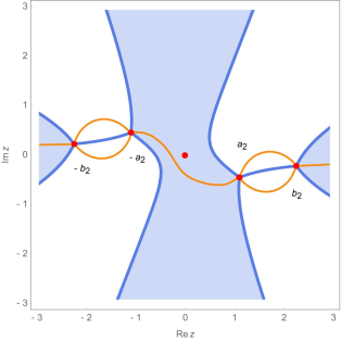
Figure 7. Schematic representation of $\Gamma\cup J^{\pm}$ superimposed on Figure 5(A)

Denote the regions bounded by $J_{t}$ and $J_{\pm}$ by $L_{\pm}$ and define

(5.3) $$\mathbf{S}_{n}(z)\mathrel{\mathop{\mathchar 58\relax}}=\mathbf{T}_{n}(z)\left\{\begin{array}[]{ll}\begin{bmatrix}1&0\\ \mp e^{-n\eta_{2}(z)-(n-N_{n})V(z)}&1\end{bmatrix}&z\in L_{\pm},\vskip 6.0pt plus 2.0pt minus 2.0pt\\ \mathbb{I},&\text{otherwise}.\end{array}\right.$$

Then, $\mathbf{S}$ solves RHP-${\mathbf{S}_{n}}$:

1. $\mathbf{S}_{n}(z)$ is analytic in ${\mathbb{C}}\setminus(\Gamma\cup J_{\pm})$ and $\lim_{{\mathbb{C}}\setminus\Gamma\ni z\to\infty}\mathbf{S}_{n}(z)=\mathbb{I}$,

2. $\mathbf{S}_{n}(z)$ has continuous traces on $\Gamma\cup J_{\pm}\setminus\{\pm a_{2},\pm b_{2}\}$ which satisfy

   $$\mathbf{S}_{n,+}(x)=\mathbf{S}_{n,-}(x)\left\{\begin{array}[]{ll}\begin{bmatrix}1&{\mathrm{e}}^{n(\eta_{2,+}(x)+(n-N_{n})V(x)}\\ 0&1\end{bmatrix},&x\in\Gamma(e^{{\mathrm{i}}\pi}\infty,-b_{2}),\vskip 6.0pt plus 2.0pt minus 2.0pt\\ \begin{bmatrix}1&{\mathrm{e}}^{n\eta_{2}(x)+(n-N_{n})V(x)}\\ 0&1\end{bmatrix},&x\in\Gamma(b_{2},{{\mathrm{e}}^{0\pi{\mathrm{i}}}}\infty),\vskip 6.0pt plus 2.0pt minus 2.0pt\\ \begin{bmatrix}{\mathrm{e}}^{n\pi{\mathrm{i}}}&{\mathrm{e}}^{n(\eta_{2,+}(x)-\pi{\mathrm{i}})+(n-N_{n})V(x)}\\ 0&{\mathrm{e}}^{-n\pi{\mathrm{i}}}\end{bmatrix},&x\in\Gamma(-a_{2},a_{2}),\vskip 6.0pt plus 2.0pt minus 2.0pt\\ \begin{bmatrix}0&{\mathrm{e}}^{(n-N_{n})V(x)}\\ -{\mathrm{e}}^{-(n-N_{n})V(x)}&0\end{bmatrix},&x\in\Gamma(-b_{2},-a_{2})\cup\Gamma(a_{2},b_{2}),\vskip 6.0pt plus 2.0pt minus 2.0pt\\ \begin{bmatrix}1&0\\ {\mathrm{e}}^{-n\eta_{2}(x)-(n-N_{n})V(x)}&1\end{bmatrix},&x\in J_{\pm}.\end{array}\right.$$

5.3. Global parametrix

If follows from the choice of contour $\Gamma$ and the discussion at the end of Section 4.3.1 (see e.g. Figure 5) that jumps of $\mathbf{S}_{n}$ on $\Gamma\setminus\Gamma(-b_{2},b_{2})$ are exponentially close to the identity, which motivates introducing the following model Riemann-Hilbert problem, RHP-${\mathbf{N}_{n}}$.

1. $\mathbf{N}_{n}(z)$ is analytic in $\overline{{\mathbb{C}}}\setminus\Gamma[-b_{2},b_{2}]$ and $\mathbf{N}(\infty)=\mathbb{I}$,

2. $\mathbf{N}_{n}(z)$ has continuous traces on $\Gamma(-b_{2},b_{2})\setminus\{\pm a_{2}\}$ which satisfy

   $$\mathbf{N}_{n,+}(x)=\mathbf{N}_{n,-}(x)\left\{\begin{array}[]{ll}\begin{bmatrix}0&{\mathrm{e}}^{(n-N_{n})V(x)}\\ -{\mathrm{e}}^{-(n-N_{n})V(x)}&0\end{bmatrix},&x\in\Gamma(-b_{2},-a_{2})\cup\Gamma(a_{2},b_{2}),\vskip 6.0pt plus 2.0pt minus 2.0pt\\ \begin{bmatrix}{\mathrm{e}}^{n\pi{\mathrm{i}}}&0\\ 0&{\mathrm{e}}^{-n\pi{\mathrm{i}}}\end{bmatrix},&x\in I_{t}.\end{array}\right.$$

We can solve RHP-${\mathbf{N}_{n}}$ in two different manners depending on the parity of $n$, and we do so in the following subsections.

5.3.1. $\mathbf{N}_{n}(z)$ when $n\in 2{\mathbb{N}}$

Let

(5.4) $$\mathbf{N}_{n}(z)\mathrel{\mathop{\mathchar 58\relax}}=\mathcal{D}^{-(N_{n}-n)\sigma_{3}}(\infty)\begin{bmatrix}A(z)&-B(z)\\ B(z)&A(z)\end{bmatrix}\mathcal{D}^{(N_{n}-n)\sigma_{3}}(z),$$

where $A(z),B(z)$, and $\mathcal{D}(z)$ are defined in (4.45) and Proposition 4.9, respectively. RHP-${\mathbf{N}_{n}}$(a) follows from the analyticity properties of $A,B,D$,(4.46), and (4.32). RHP-${\mathbf{N}_{n}}$(b) follows from (4.47) and (4.31).

5.3.2. $\mathbf{N}_{n}(z)$ when $n\in{\mathbb{N}}\setminus 2{\mathbb{N}}$

Let

$$\mathbf{M}_{n}(z)\mathrel{\mathop{\mathchar 58\relax}}=\begin{bmatrix}(A/\Theta^{(0)})(z)&-(B/\Theta^{(1)})(z)\\ (\Theta^{(0)}B)(z)&(\Theta^{(1)}A)(z)\end{bmatrix}\mathcal{D}^{(N_{n}-n)\sigma_{3}}(z)$$

where $\Theta$ is defined in (4.42). It follows from analyticity properties of $\Theta$ and Proposition 4.11 that $\Theta^{(0)}(\infty)$ and consequently $\Theta^{(1)}(\infty)$ are finite and nonvanishing. Then, combining this with (4.46) and boundedness/nonvanishing of $\mathcal{D}(\infty)$, we have that $\mathbf{M}(\infty)$ exists and

$$\lim_{z\to\infty}\det\mathbf{M}_{n}(z)=\dfrac{\Theta^{(1)}(\infty)}{\Theta^{(0)}(\infty)}>0.$$

Hence, the matrix

(5.5) $$\mathbf{N}_{n}(z)\mathrel{\mathop{\mathchar 58\relax}}=\mathbf{M}_{n}^{-1}(\infty)\mathbf{M}_{n}(z),$$

exists for all $n\in{\mathbb{N}}\setminus 2{\mathbb{N}}$. Furthermore, $\mathbf{N}_{n}$ satisfies RHP-${\mathbf{N}_{n}}$(a) due to the analyticity properties of $\Theta$, $A,B,$ and $D$. RHP-${\mathbf{N}_{n}}$(b) follows from (4.31), (4.47), and (4.43).

It will be useful to note that it follows from formulas (5.4), (5.5) that

1. for any $e\in\{\pm a_{2},\pm b_{2}\}$, we have that $\mathbf{N}_{n}(z)=\mathbf{O}\left[|z-e|^{-1/4}\right]$ as $z\to e$, and

2. $\det\left(\mathbf{N}_{n}(z)\right)=1$.

Indeed, (i) follows immediately from the definition of $A,B,D$ and $\Theta$. For (ii), note that $\det\left(\mathbf{N}_{n}(z)\right)$ is an analytic function in ${\mathbb{C}}\setminus\{\pm a_{2},\pm b_{2}\}$. Furthermore, $\det\left(\mathbf{N}_{n}(z)\right)$ has at most square root growth at each of $\{\pm a_{2},\pm b_{2}\}$, making them removable singularities. Applying Liouville’s theorem yields $\det\left(\mathbf{N}_{n}(z)\right)$ is constant, and the normalization at infinity implies (ii).

5.4. Local parametrices

To handle the fact that the jumps removed in RHP-${\mathbf{N}_{n}}$ are not uniformly close to identity, we construct parametrices near the endpoints $\{\pm a_{2},\pm b_{2}\}$ which solve RHP-${\mathbf{S}_{n}}$ in a neighborhood $U_{e},\ e\in\{\pm a_{2},\pm b_{2}\}$ exactly. Furthermore, we require that this local solution “matches” the global parametrix on $\partial U_{e}$. Specifically, fix $e\in\{\pm a_{2},\pm b_{2}\}$ and let

$$U_{e}\mathrel{\mathop{\mathchar 58\relax}}=\{z\ \mathrel{\mathop{\mathchar 58\relax}}\ |z-e|<\delta_{e}(t)\},$$

where $\delta_{e}$ where $\delta_{e}(t)$ is a radius to be determined. We seek a solution to the following RHP-${\mathbf{P}_{e,n}}$

1. $\mathbf{P}_{e,n}(z)$ has the same analyticity properties as $\mathbf{S}_{n}(z)$ restricted to $U_{e}$, see RHP-${\mathbf{S}_{n}}$(a);

2. $\mathbf{P}_{e,n}(z)$ satisfies the same jump relations as $\mathbf{S}_{n}(z)$ restricted to $U_{e}$, see RHP-${\mathbf{S}_{n}}$(b);

3. $\mathbf{P}_{e,n}(z)=\mathbf{N}_{n}(z)\left(\mathbb{I}+\mathbf{O}(n^{-1})\right)$ holds uniformly on $\partial U_{e}$ as $n\to\infty$.

5.4.1. Model Parametrix.

Let $\mathbf{A}(\zeta)$ be an analytic matrix-valued function in ${\mathbb{C}}\setminus\big{(}(-\infty,\infty)\cup L_{-}\cup L_{+}\big{)}$, $L_{\pm}\mathrel{\mathop{\mathchar 58\relax}}=\big{\{}\zeta\mathrel{\mathop{\mathchar 58\relax}}~{}\text{arg}(\zeta)=\pm 2\pi/3\big{\}}$ satisfying

$$\mathbf{A}_{+}(s)=\mathbf{A}_{-}(s)\left\{\begin{array}[]{ll}\begin{bmatrix}0&1\\ -1&0\end{bmatrix},&s\in(-\infty,0),\vskip 6.0pt plus 2.0pt minus 2.0pt\\ \begin{bmatrix}1&0\\ 1&1\end{bmatrix},&s\in L_{\pm},\vskip 6.0pt plus 2.0pt minus 2.0pt\\ \begin{bmatrix}1&1\\ 0&1\end{bmatrix},&s\in(0,\infty),\end{array}\right.$$

where the real line is oriented from $-\infty$ to $\infty$ and the rays $L_{\pm}$ are oriented towards the origin. This problem was solved explicitly [MR1702716, MR1858269] (see also [MR1677884]) in terms of Airy functions, and henceforth we denote this solution by $\mathbf{A}(\zeta)$. It is known that $\mathbf{A}(\zeta)$ has the following asymptotic expansion at infinity:

(5.6) $$\mathbf{A}(\zeta)e^{\frac{2}{3}\zeta^{3/2}\sigma_{3}}\sim\frac{\zeta^{-\sigma_{3}/4}}{\sqrt{2}}\sum_{k=0}^{\infty}\begin{bmatrix}s_{k}&0\\ 0&t_{k}\end{bmatrix}\begin{bmatrix}(-1)^{k}&\mathrm{i}\\ (-1)^{k}\mathrm{i}&1\end{bmatrix}\left(\frac{2}{3}\zeta^{3/2}\right)^{-k},$$

uniformly in ${\mathbb{C}}\setminus\big{(}(-\infty,\infty)\cup L_{-}\cup L_{+}\big{)}$, where

$$s_{0}=t_{0}=1,\quad s_{k}=\frac{\Gamma(3k+1/2)}{54^{k}k!\Gamma(k+1/2)},\quad t_{k}=-\frac{6k+1}{6k-1}s_{k},\quad k\geq 1.$$

5.4.2. Local coordinates.

In this section, it will be convenient to denote

(5.7) $$J_{e}\mathrel{\mathop{\mathchar 58\relax}}=J_{\sigma}\cap U_{e},\quad I_{e}\mathrel{\mathop{\mathchar 58\relax}}=\left(\Gamma\cap U_{e}\right)\setminus J_{e}.$$

To transform RHP-${\mathbf{P}_{e,n}}$ to the model problem above, we will need to study the function $\eta_{2,e}$ as $z\to e$. To this end, observe that the choice of of $\Gamma_{t}$ in Theorem 4.7 implies

$$\eta_{2,e}(z)<0\quad\text{for}\quad z\in I_{e},$$

and that

$$\eta_{2,e}(z)=\pm 2\pi{\mathrm{i}}\varsigma(e)\mu_{t}\left(\Gamma_{t}[e,z]\right)={\mathrm{e}}^{\mp\varsigma(e)3\pi{\mathrm{i}}/2}2\pi\mu_{t}\left(\Gamma_{t}[e,z]\right),\quad z\in J_{e}$$

where

(5.8) $$\varsigma(e)=\left\{\begin{array}[]{ll}-1,&e\in\{-b_{2},a_{2}\},\\ 1,&e\in\{b_{2},-a_{2}\}.\end{array}\right.$$

In particular, since $\eta_{2,e}(z)\sim|z-e|^{3/2}$ as $z\to e$, we may define a holomorphic branch of $\zeta_{e}(z)\mathrel{\mathop{\mathchar 58\relax}}=(-3n\eta_{2,e}(z)/4)^{2/3}$ so that $\eta_{2,e}(I_{e})\subseteq(0,\infty)$, $\eta_{2,e}(J_{e})\subseteq(-\infty,0)$, and $\eta_{2,e}$ is conformal in a sufficiently small neighborhood of $e$; we choose $\delta_{e}(t)>0$ so that $\eta_{2,e}$ is conformal in $U_{e}$.

Remark 5.1.

We note that for any given compact $K\subseteq\mathcal{O}_{2}$, we may (and will) choose $\delta_{e}(t)$ so that they are continuous and separated from zero on $K$ by, say, choosing $2\delta_{e}(t)=\left(\min\{2\pi,|\eta_{2,e}(0)|\}\right)^{2/3}$. This follows from the Basic Structure Theorem [MR0096806]*Theorem 3.5 and arguments carries out in [MR3607591]*Section 6.4. One of the main technical difficulties of extending our asymptotic results to hold uniformly on unbounded subsets of $\mathcal{O}_{2}$ is choosing such radii that remain bounded away from zero as $t\to\infty$. This was done in [MR3607591]*Section 6.4 and requires careful estimates of the quantity $\delta_{e}(t)$ above. While similar analysis can be carries out here, for the sake of brevity we settle for locally uniform asymptotics.

5.4.3. Solution of RHP-${\mathbf{P}_{e,n}}$.

Let

(5.9) $$\mathbf{P}_{e,n}(z)\mathrel{\mathop{\mathchar 58\relax}}=\mathbf{E}_{e}(z)\mathbf{A}_{e}(\zeta_{e}(z)){\mathrm{e}}^{\frac{2}{3}\zeta^{3/2}_{e}(z)\sigma_{3}}\mathbf{J}_{e}(z),$$

where

• $\mathbf{E}_{e}(z)$ is a holomorphic prefactor to be determined,

• $\mathbf{A}_{e}(\zeta)\mathrel{\mathop{\mathchar 58\relax}}=\mathbf{A}(\zeta)$ for $e\in\{-a_{2},b_{2}\}$ and $\mathbf{A}_{e}(\zeta)\mathrel{\mathop{\mathchar 58\relax}}=\sigma_{3}\mathbf{A}(\zeta)\sigma_{3}$ otherwise. The conjugation by $\sigma_{3}$ has the effect of reversing the orientation of ${\mathbb{R}}\cup L_{\pm}$,

• we define

  $$\mathbf{J}_{e}(z)\mathrel{\mathop{\mathchar 58\relax}}={\mathrm{e}}^{(N_{n}-n)V(z)\sigma_{3}/2}\left\{\begin{array}[]{ll}\mathbb{I},&e\in\{\pm b_{2}\},\\ {\mathrm{e}}^{\pm\pi{\mathrm{i}}n\sigma_{3}/2},&e\in\{\pm a_{2}\},\end{array}\right.$$

  and we choose the $+/-$ sign when $z$ is to the left/right of $\Gamma$, respectively.

Indeed, RHP-${\mathbf{P}_{e,n}}$(a) follows directly from the analyticity properties of $\mathbf{A}_{e}$, $\mathbf{J}_{e}$, and $\zeta_{e}$. Using (4.18), (4.27), (4.28), and (4.21), we see that for any $e\in\{\pm a_{2},\pm b_{2}\}$

(5.10) $$(g_{+}+g_{-}-V-\ell^{(2)}_{*})(z)=\dfrac{1}{2}\left(\eta_{e,+}+\eta_{e,-}\right)(z),\quad z\in\Gamma$$

and

(5.11) $$(g_{+}-g_{-})(z)=\dfrac{1}{2}\left(\eta_{e,+}-\eta_{e,-}\right)(z)+\left\{\begin{array}[]{ll}0,&e=b_{2},\\ \pi{\mathrm{i}},&e\in\{\pm a_{2}\},\\ 2\pi{\mathrm{i}},&e=-b_{2},\end{array}\right.\quad z\in\Gamma.$$

Using (5.11) along with (4.27), (4.28), one may directly verify RHP-${\mathbf{P}_{e,n}}$(b). Finally, to satisfy RHP-${\mathbf{P}_{e,n}}$(c), we choose

$$\mathbf{E}_{e}(z)\mathrel{\mathop{\mathchar 58\relax}}=\mathbf{N}_{n}(z)\mathbf{J}_{e}^{-1}(z)\dfrac{1}{\sqrt{2}}\begin{bmatrix}1&-{\mathrm{i}}\varsigma(e)\\ -{\mathrm{i}}\varsigma(e)&1\end{bmatrix}\zeta_{e}^{1/4}(z),$$

where $\varsigma(e)$ is as as in (5.8). It follows from the definition of $\mathbf{N},\mathbf{J}_{e}$, and jump conditions RHP-${\mathbf{N}_{n}}$(b) that $\mathbf{E}_{e}$ is analytic in $U_{e}\setminus\{e\}$. At $z=e$, it follows from the discussion in Section 5.3 and the conformality of $\zeta_{e}$ that $\mathbf{E}_{e}$ has at most a square-root singularity at $e$, making it a removable singularity and yielding the desired analyticity.

Using (5.6), the definition of $\mathbf{P}_{e,n}(z)$, and the definition of $\mathbf{E}_{e}(z)$, it follows that for $z\in\partial U_{e}$,

(5.12) $$\mathbf{P}_{e,n}(z)\sim\mathbf{N}_{n}(z)\left(\mathbb{I}+\dfrac{1}{n}\sum_{k=0}^{\infty}\dfrac{\mathbf{C}_{e,k}(z)}{n^{k}}\right)\quad\text{as}\quad n\to\infty.$$

where $\mathbf{C}_{e,k}(z)$ can be explicitly calculated, but we will not use these formulas and so omit them. We point out that the $\mathbf{C}_{e,k}(z)$ depend on $t$ via $\eta_{2,e}(z;t)$ and $V(z;t)$ and are thus continuous in $t$.

5.5. Small-norm Riemann-Hilbert problem

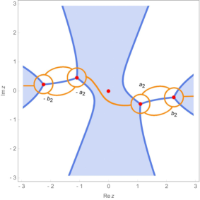
Figure 8. Schematic representation of $\Sigma$ (orange) superimposed on Figure 5(A)

Let

$$\Sigma=\left[\left(\Gamma\cup J_{t}\cup J_{+}\cup J_{-}\right)\cap({\mathbb{C}}\setminus\cup_{e}U_{e})\right]\cup\left(\cup_{e}\partial U_{e}\right),$$

shown schematically in Figure 8. Consider the following Riemann-Hilbert problem RHP-${\mathbf{R}_{n}}$:

1. $\mathbf{R}_{n}(z)$ is holomorphic in ${\mathbb{C}}\setminus\Sigma$ and $\lim_{{\mathbb{C}}\setminus\Gamma\ni z\to\infty}\mathbf{R}_{n}(z)=\mathbb{I}$,

2. $\mathbf{R}_{n}(z)$ has continuous traces on points of $\Sigma$ with a well-defined tangent line that satisfy

   $$\mathbf{R}_{n,+}(x)=\mathbf{R}_{n,-}(x)\left\{\begin{array}[]{ll}\mathbf{P}_{e,n}(x)\mathbf{N}_{n}^{-1}(x),&x\in\partial U_{e},\vskip 6.0pt plus 2.0pt minus 2.0pt\\ \mathbf{N}_{n}(x)\begin{bmatrix}1&0\\ {\mathrm{e}}^{-n\eta_{2}(x)-(n-N_{n})V(s)}&1\end{bmatrix}\mathbf{N}_{n}^{-1}(x),&s\in J_{\pm}\cap{\mathbb{C}}\setminus\cup_{e}U_{e}.\end{array}\right.$$

   where $\partial U_{e}$ are oriented clockwise, and (recall that $\det\mathbf{N}_{n}(z)=1$, see Section 5.3)

   $$\mathbf{R}_{n,+}(x)=\mathbf{R}_{n,-}(x)\left\{\begin{array}[]{ll}\mathbf{N}_{n}(x)\begin{bmatrix}1&{\mathrm{e}}^{n(\eta_{2,+}(x)+(n-N_{n})V(x)}\\ 0&1\end{bmatrix}\mathbf{N}_{n}^{-1}(x),&x\in\Gamma(e^{{\mathrm{i}}\pi}\infty,-b_{2}),\vskip 6.0pt plus 2.0pt minus 2.0pt\\ \mathbf{N}_{n}(x)\begin{bmatrix}{\mathrm{e}}^{-n\eta_{2,+}(x)}&{\mathrm{e}}^{(n-N_{n})V(x)}\\ 0&{\mathrm{e}}^{n\eta_{2,+}(x)}\end{bmatrix}\mathbf{N}_{n}^{-1}(x),&x\in\Gamma(-b_{2},-a_{2}),\vskip 6.0pt plus 2.0pt minus 2.0pt\\ \mathbf{N}_{n}(x)\begin{bmatrix}1&{\mathrm{e}}^{n\eta_{2}(x)+(n-N_{n})V(x)}\\ 0&1\end{bmatrix}\mathbf{N}_{n}^{-1}(x),&x\in\Gamma(b_{2},{{\mathrm{e}}^{0\pi{\mathrm{i}}}}\infty),\vskip 6.0pt plus 2.0pt minus 2.0pt\\ \mathbf{N}_{n,-}(x)\begin{bmatrix}{\mathrm{e}}^{n\pi{\mathrm{i}}}&{\mathrm{e}}^{n(\eta_{2,+}(x)-\pi{\mathrm{i}})+(n-N_{n})V(x)}\\ 0&{\mathrm{e}}^{-n\pi{\mathrm{i}}}\end{bmatrix}\mathbf{N}^{-1}_{n,+}(x),&x\in I_{t},\vskip 6.0pt plus 2.0pt minus 2.0pt\\ \mathbf{N}_{n}(x)\begin{bmatrix}{\mathrm{e}}^{-n\eta_{2,+}(x)}&{\mathrm{e}}^{(n-N_{n})V(x)}\\ 0&{\mathrm{e}}^{n\eta_{2,+}(x)}\end{bmatrix}\mathbf{N}_{n}^{-1}(x),&x\in\Gamma(a_{2},b_{2}).\end{array}\right.$$

We now show that $\mathbf{R}_{n}$ satisfies a so-called ”small-norm” Riemann-Hilbert problem. The estimates in this section are fairly well-known at this point, but since we also consider the dependence on the parameter $t$, we point to [MR3607591]*Section 7.6 as a general reference. Consider

(5.13) $$\mathbf{\Delta}(x)\mathrel{\mathop{\mathchar 58\relax}}=(\mathbf{R}_{n,-}^{-1}\mathbf{R}_{n,+})(x)-\mathbb{I},\quad x\in\Sigma.$$

It follows from the explicit formulas in Section 5.3 that $\mathbf{N}_{n}$ is uniformly bounded on $\Sigma$. This, the choice of $\Gamma$ (see equation (4.29) and the surrounding discussion), the fact that $|n-N_{n}|$ is bounded for all $n\in{\mathbb{N}}$, and the jump of $\mathbf{N}_{n}$ on $I_{t}$ implies that there exists $c(t;\delta)>0$, where $\delta=\min_{e}\delta_{e}$, so that as $n\to\infty$

(5.14) $$\mathbf{\Delta}(x,t)=\mathcal{O}\left({\mathrm{e}}^{-c(t;\delta)n}\right)\quad\text{for}\quad x\in(J_{\pm}\cap({\mathbb{C}}\setminus\cup_{e}U_{e}))\cup I_{t}\cup\Gamma(-\infty,-b_{2})\cup\Gamma(b_{2},\infty).$$

Since $\Delta(x;t)$ is continuous in $t$, we can choose the exponent $c(t;\delta)$ to be continuous in $t$ as well, and by compactness we find that (5.14) holds $(x,t)$-locally uniformly. Similarly, by (5.12) and the definition of $\mathbf{\Delta}$, it follows that for $x\in\partial U_{e}$

(5.15) $$\mathbf{\Delta}(x;t)\sim\sum_{k=1}^{\infty}\dfrac{\mathbf{N}_{n}(x;t)\mathbf{C}_{e,k}(x;t)\mathbf{N}_{n}^{-1}(x;t)}{n^{k}}\quad\text{as}\quad n\to\infty$$

Once again, by continuity we have that estimate (5.15) holds $(x,t)$-locally uniformly. Put together, the above estimates yield that $\|\mathbf{\Delta}\|_{L^{\infty}(\Sigma)}=\mathcal{O}\left(n^{-1}\right)$ $t$-locally uniformly. Furthermore, on the unbounded components of $\Sigma$ we have

$$\mathbf{\Delta}(x;t)=\mathbf{N}_{n}(x;t)\begin{bmatrix}1&{\mathrm{e}}^{n(\eta_{2,+}(x;t)+(n-N_{n})V(x;t)}\\ 0&1\end{bmatrix}\mathbf{N}_{n}^{-1}(x;t),$$

and since $\mathbf{N}_{n}$ is bounded as $x\to\infty$ and ${\mathrm{e}}^{n\eta_{2}(x;t)}$ is exponentially small as $x\to\infty$, it follows that

(5.16) $$\|\mathbf{\Delta}\|_{L^{\infty}(\Sigma)\cap L^{2}(\Sigma)}=\mathcal{O}\left(n^{-1}\right).$$

Hence, applying [MR1677884]*Corollary 7.108, yields that for $n$ large enough, a solution $\mathbf{R}_{n}$ exists and

(5.17) $$\mathbf{R}_{n}(z)=\mathbb{I}+\mathcal{O}\left(\dfrac{1}{n}\right)\quad\text{as}\quad n\to\infty,$$

$(z,t)$-uniformly in ${\mathbb{C}}$. In the next subsection, we use this to conclude asymptotic formulas for polynomials $P_{n}(z;t,N_{n})$ and recurrence coefficients $\gamma^{2}_{n}(t,N_{n})$.

5.6. Asymptotics of $P_{n}(z;t)$.

Given $\mathbf{R}_{n}(z)$, $\mathbf{N}_{n}(z)$, and $\mathbf{P}_{e,n}(z)$, solutions of RHP-${\mathbf{R}_{n}}$, RHP-${\mathbf{N}_{n}}$, and RHP-${\mathbf{P}_{e,n}}$, respectively, one can verify that RHP-${\mathbf{S}_{n}}$ is solved by

(5.18) $$\mathbf{S}_{n}(z)=\left\{\begin{array}[]{ll}(\mathbf{R}_{n}\mathbf{N}_{n})(z),&\quad({\mathbb{C}}\setminus\overline{U}_{e})\setminus[(\Gamma\setminus J_{t})\cup J_{+}\cup J_{-}],\vskip 6.0pt plus 2.0pt minus 2.0pt\\ (\mathbf{R}_{n}\mathbf{P}_{e,n})(z),&\quad U_{e},~{}~{}~{}e\in\{\pm a_{2},\pm b_{2}\}.\end{array}\right.$$

Let $K$ be a compact set in ${\mathbb{C}}\setminus\Gamma$. We can always arrange so that the set $K$ lies entirely within the unbounded component of the contour $\Sigma$. Then it follows from (5.2), (5.3), and (5.18) that

(5.19) $$\mathbf{Y}_{n}(z)={\mathrm{e}}^{n\ell_{*}^{(2)}\sigma_{3}/2}(\mathbf{R}_{n}\mathbf{N}_{n})(z){\mathrm{e}}^{n(g(z)-\ell_{*}^{(2)}/2)\sigma_{3}},\quad z\in K.$$

Subsequently, by using (5.1) and (4.18), we see that

$$P_{n}(z)=[\mathbf{Y}(z)]_{11}={\mathrm{e}}^{\frac{n}{2}(\eta_{2}(z)+V(z)+\ell^{(2)}_{*})}\left([\mathbf{R}_{n}(z)]_{11}[\mathbf{N}_{n}(z)]_{11}+[\mathbf{R}_{n}(z)]_{12}[\mathbf{N}_{n}(z)]_{21}\right).$$

Using formulas (5.4), (5.5), estimate (5.17), and the definitions of the entries of $\mathbf{N}_{n}$ yields (4.48).

5.7. Asymptotics of $\gamma_{n}^{2}(t)$

It follows from Theorem 4.13 that for $n$ large enough, $\text{deg}P_{n}=n$, and in this section we will use the notation

$$P_{n}(z;t,N)=z^{n}+\sum_{k=0}^{n-1}\mathfrak{p}_{n,k}(t,N)z^{k}.$$

Furthermore, we will drop the $n$ subscript (e.g. $\mathbf{N}_{n}\mapsto\mathbf{N}$) and use notation

$$\mathbf{K}(z)=\mathbb{I}+z^{-1}\mathbf{K}_{1}(n,t,N)+z^{-2}\mathbf{K}_{2}(n,t,N)+z^{-3}\mathbf{K}_{3}(n,t,N)+\mathcal{O}\big{(}z^{-4}\big{)}\quad\text{as}\quad z\to\infty,$$

where $\mathbf{K}\in\{\mathbf{M},\mathbf{N},\mathbf{R},\mathbf{T},\mathbf{Y}z^{-n\sigma_{3}}\}$. It follows from the orthogonality relations (1.5) and (1.10) that

$$z^{n}\big{(}\mathcal{C}P_{n}{\mathrm{e}}^{-NV}\big{)}(z) =-\frac{1}{z}\frac{1}{2\pi{\mathrm{i}}}\int_{\Gamma}x^{n}P_{n}(x){\mathrm{e}}^{-NV(x)}{\mathrm{d}}x-\frac{1}{z^{2}}\frac{1}{2\pi{\mathrm{i}}}\int_{\Gamma}x^{n+1}P_{n}(x){\mathrm{e}}^{-NV(x)}{\mathrm{d}}x+\mathcal{O}\left(z^{-3}\right)$$

$$=\frac{h_{n}(t,N)}{2\pi{\mathrm{i}}}\left(-\frac{1}{z}+\frac{\mathfrak{p}_{n+1,n}(t,N)}{z^{2}}\right)+\mathcal{O}\left(z^{-3}\right),$$

where the second expression for the coefficient next to $z^{-2}$ follows from the observation

$$\int_{\Gamma}x^{n+1}P_{n}(x){\mathrm{e}}^{-NV(x)}{\mathrm{d}}x\\ =\int_{\Gamma}\left(x^{n+1}-P_{n+1}(x)\right)P_{n}(x){\mathrm{e}}^{-NV(x)}{\mathrm{d}}x=\mathfrak{p}_{n+1,n}(t,N)\int x^{n}P_{n}(x){\mathrm{e}}^{-NV(x)}{\mathrm{d}}x,$$

where all polynomials correspond to the same parameter $N$. However, since the weight of orthogonality is an even function, we have $P_{n}(-z;t,N)=(-1)^{n}P_{n}(z;t,N)$, i.e. polynomials $P_{n}$ are even/odd functions. In particular $\mathfrak{p}_{n+1,n}(t,N)=0$. Hence, it follows from (5.1) that

(5.20) $${\mathbf{Y}}_{1}(n,t,N) =\begin{bmatrix}0&-\frac{h_{n}(t,N)}{2\pi{\mathrm{i}}}\vskip 6.0pt plus 2.0pt minus 2.0pt\\ -\frac{2\pi{\mathrm{i}}}{h_{n-1}(t,N)}&0\end{bmatrix}$$

$$\mathbf{Y}_{2}(n,t,N) =\begin{bmatrix}\mathfrak{p}_{n,n-2}(t,N)&0\vskip 6.0pt plus 2.0pt minus 2.0pt\\ 0&*\end{bmatrix},$$

$$\mathbf{Y}_{3}(n,t,N) =\begin{bmatrix}0&*\vskip 6.0pt plus 2.0pt minus 2.0pt\\ -\frac{2\pi{\mathrm{i}}}{h_{n-1}(t,N)}\mathfrak{p}_{n-1,n-3}(t,N)&*\end{bmatrix}.$$

This along with (1.9) yields the formulae

(5.21) $$\begin{cases}h_{n}(t,N)&=-2\pi{\mathrm{i}}[\mathbf{Y}_{1}(n,t,N)]_{12},\vskip 6.0pt plus 2.0pt minus 2.0pt\\ \gamma_{n}^{2}(t,N)&=[\mathbf{Y}_{1}(n,t,N)]_{12}[\mathbf{Y}_{1}(n,t,N)]_{21},\vskip 6.0pt plus 2.0pt minus 2.0pt\\ \mathfrak{p}_{n,n-2}(t,N)&=[\mathbf{Y}_{2}(n,t,N)]_{11},\vskip 6.0pt plus 2.0pt minus 2.0pt\\ \mathfrak{p}_{n-1,n-3}(t,N)&=\dfrac{[\mathbf{Y}_{3}(n,t,N)]_{21}}{[\mathbf{Y}_{1}(n,t,N)]_{21}}.\end{cases}$$

Next, using (4.23) we have

(5.22) $${\mathrm{e}}^{-ng(z)\sigma_{3}}=z^{-n\sigma_{3}}\left(\mathbb{I}-\dfrac{nt}{2z^{2}}\sigma_{3}+{\mathcal{O}}\left(\dfrac{1}{z^{4}}\right)\right).$$

Combining (5.22) with (5.2) yields

(5.23) $$\begin{cases}[\mathbf{T}_{1}(n,t,N)]_{12}&={\mathrm{e}}^{-n\ell^{(2)}_{*}}[\mathbf{Y}_{1}(n,N)]_{12},\vskip 6.0pt plus 2.0pt minus 2.0pt\\ [\mathbf{T}_{1}(n,t,N)]_{21}&={\mathrm{e}}^{n\ell^{(2)}_{*}}[\mathbf{Y}_{1}(n,t,N)]_{21},\vskip 6.0pt plus 2.0pt minus 2.0pt\\ [\mathbf{T}_{1}(n,t,N)]_{11}&=[\mathbf{Y}_{1}(n,t,N)]_{11},\vskip 6.0pt plus 2.0pt minus 2.0pt\\ [\mathbf{T}_{2}(n,t,N)]_{11}&=[\mathbf{Y}_{2}(n,t,N)]_{11}-\dfrac{nt}{2},\vskip 6.0pt plus 2.0pt minus 2.0pt\\ [\mathbf{T}_{3}(n,t,N)]_{21}&={\mathrm{e}}^{n\ell_{*}^{(2)}}\left([\mathbf{Y}_{3}(n,t,N)]_{21}-\dfrac{nt}{2}[\mathbf{Y}_{1}(n,t,N)]_{21}\right).\end{cases}$$

This, in turn, leads to

(5.24) $$\left\{\begin{array}[]{lll}h_{n}(t,N)&=&-2\pi{\mathrm{i}}{\mathrm{e}}^{n\ell^{(2)}_{*}}[\mathbf{T}_{1}(n,N)]_{12},\vskip 6.0pt plus 2.0pt minus 2.0pt\\ \gamma_{n}^{2}(t,N)&=&[\mathbf{T}_{1}(n,t,N)]_{12}[\mathbf{T}_{1}(n,t,N)]_{21},\vskip 6.0pt plus 2.0pt minus 2.0pt\\ \mathfrak{p}_{n,n-2}(t,N)&=&[\mathbf{T}_{2}(n,t,N)]_{11}+\dfrac{nt}{2},\vskip 6.0pt plus 2.0pt minus 2.0pt\\ \mathfrak{p}_{n-1,n-3}(t,N)&=&\dfrac{[\mathbf{T}_{3}(n,t,N)]_{21}}{[\mathbf{T}_{1}(n,t,N)]_{21}}+\dfrac{nt}{2}.\par\end{array}\right.$$

It was shown in [MR1711036]*Theorem 7.10 that $\mathbf{R}(z)$ admits an asymptotic expansion (in the sense of Footnote 19)

(5.25) $$\mathbf{R}(z)\sim\mathbb{I}+\sum_{k=1}^{\infty}\dfrac{\mathbf{R}^{(k)}(z,n)}{n^{k}},\quad n\to\infty\quad\text{ and }\quad z\in{\mathbb{C}}\setminus\cup_{e}\partial U_{e}.$$

The matrices $\mathbf{R}^{(k)}(z)$ satisfy an additive Riemann-Hilbert Problem:

1. $\mathbf{R}^{(k)}(z)$ is analytic in ${\mathbb{C}}\setminus\cup_{e}\partial U_{e}$;

2. $\mathbf{R}_{+}^{(k)}(z)=\mathbf{R}_{-}^{(k)}(z)+\sum_{j=1}^{k}\mathbf{R}_{-}^{(k-j)}(z)\mathbf{\Delta}_{j}(z)$ for $z\in\cup_{e}\partial U_{e}$, where we write

   $$\mathbf{\Delta}(z)\sim\sum_{k=1}^{\infty}\dfrac{\mathbf{\Delta}_{k}}{n^{k}}\quad\text{as}\quad n\to\infty,$$

   and $\mathbf{\Delta}$ is as in (5.13);

3. as $z\to\infty,$ $\mathbf{R}^{(k)}(z)$ admits an expansion of the form

   (5.26) $$\mathbf{R}^{(k)}(z)=\dfrac{\mathbf{R}_{1}^{(k)}}{z}+\dfrac{\mathbf{R}_{2}^{(k)}}{z^{2}}+\mathcal{O}\left(\dfrac{1}{z^{3}}\right).$$

Recall that $\mathbf{T}(z)=(\mathbf{R}\mathbf{N})(z)$ for $z$ in the vicinity of infinity by (5.2) and (5.19). It also follows from their definitions that matrices $\mathbf{N}(z)$ form a normal family in $n\in{\mathbb{N}}$ in the vicinity of infinity. Plugging expansions (5.25) and (5.26) into the product $\mathbf{T}(z)=(\mathbf{R}\mathbf{N})(z)$ yields

(5.27) $$\mathbf{T}_{1}(n,t,N_{n}) =\mathbf{N}_{1}(n,t,N_{n})+\dfrac{\mathbf{R}^{(1)}_{1}(t)}{n}+\mathcal{O}\left(\dfrac{1}{n^{2}}\right),\vskip 6.0pt plus 2.0pt minus 2.0pt$$

$$\mathbf{T}_{2}(n,t,N_{n}) =\mathbf{N}_{2}(n,t,N_{n})+\dfrac{\mathbf{R}_{1}^{(1)}(t)\mathbf{N}_{1}(n,t,N_{n})+\mathbf{R}_{2}^{(1)}(t)}{n}+\mathcal{O}\left(\dfrac{1}{n^{2}}\right),\vskip 6.0pt plus 2.0pt minus 2.0pt$$

$$\mathbf{T}_{3}(n,t,N_{n}) =\mathbf{N}_{3}(n,t,N_{n})+\dfrac{\mathbf{R}_{1}^{(1)}(t)\mathbf{N}_{2}(n,t,N_{n})+\mathbf{R}_{2}^{(1)}(t)\mathbf{N}_{1}(n,t,N_{n})+\mathbf{R}_{3}^{(1)}(t)}{n}+\mathcal{O}\left(\dfrac{1}{n^{2}}\right).$$

where normality of $\mathbf{N}$ is used to ensure boundedness of coefficients $\mathbf{N}_{k}(n,t,N)$. To use (5.27), we will need to compute $\mathbf{N}_{1},\mathbf{N}_{2},\mathbf{N}_{3}$. To this end, note that by (4.32),

(5.28) $$\mathcal{D}^{(N-n)\sigma_{3}}(z)={\mathrm{e}}^{-(N-n)\ell_{*}^{(2)}\sigma_{3}/2}\left(\mathbb{I}+\dfrac{N-n}{4z^{4}}\sigma_{3}+\mathcal{O}\left(\dfrac{1}{z^{6}}\right)\right).$$

Furthermore, it follows from the definition of $\gamma(z)$ in (4.44) that

$$\gamma(z) =1+\dfrac{a_{2}-b_{2}}{2z}+\dfrac{(a_{2}-b_{2})^{2}}{8z^{2}}+\dfrac{(a_{2}-b_{2})(3a_{2}^{2}+2a_{2}b_{2}+3b_{2}^{2})}{16z^{3}}+\mathcal{O}\left(\dfrac{1}{z^{3}}\right)\quad\text{as}\quad z\to\infty,$$

$$\gamma^{-1}(z) =1-\dfrac{a_{2}-b_{2}}{2z}+\dfrac{(a_{2}-b_{2})^{2}}{8z^{2}}-\dfrac{(a_{2}-b_{2})(3a_{2}^{2}+2a_{2}b_{2}+3b_{2}^{2})}{16z^{3}}+\mathcal{O}\left(\dfrac{1}{z^{4}}\right)\quad\text{as}\quad z\to\infty,$$

which, in turn, yields

(5.29) $$A(z) =1+\dfrac{(a_{2}-b_{2})^{2}}{8z^{2}}+\mathcal{O}\left(\dfrac{1}{z^{4}}\right),$$

$$B(z) =\dfrac{a_{2}-b_{2}}{2{\mathrm{i}}z}+\dfrac{(a_{2}-b_{2})(3a_{2}^{2}+2a_{2}b_{2}+3b_{2}^{2})}{16{\mathrm{i}}z^{3}}+\mathcal{O}\left(\dfrac{1}{z^{5}}\right),\quad\text{as}\quad z\to\infty.$$

Put together, the expansions (5.28), (5.29) along with the definition of $\mathbf{N}$ yield that

(5.30) $$\mathbf{N}_{1}(n,t,N)=\dfrac{b_{2}-a_{2}}{2}{\mathrm{e}}^{(N-n)\ell_{*}^{(2)}\sigma_{3}}\sigma_{2},$$

when $n\in 2\mathbb{N}$. Recalling Proposition 4.11, we can write

(5.31) $$\mathbf{N}_{1}(n,t,N)={\mathrm{e}}^{(N-n)\ell_{*}^{(2)}\sigma_{3}/2}\begin{bmatrix}-\dfrac{{\mathrm{d}}}{{\mathrm{d}}x}\left(\log\Theta^{(0)}(1/x)\right)\biggl{|}_{x=0}&-\dfrac{a_{2}-b_{2}}{2{\mathrm{i}}}\dfrac{\Theta^{(0)}(\infty)}{\Theta^{(1)}(\infty)}\vskip 6.0pt plus 2.0pt minus 2.0pt\\ \dfrac{a_{2}-b_{2}}{2{\mathrm{i}}}\dfrac{\Theta^{(0)}(\infty)}{\Theta^{(1)}(\infty)}&\dfrac{{\mathrm{d}}}{{\mathrm{d}}x}\left(\log\Theta^{(1)}(1/x)\right)\biggl{|}_{x=0}\end{bmatrix}{\mathrm{e}}^{-(N-n)\ell_{*}^{(2)}\sigma_{3}/2},$$

when $n\in{\mathbb{N}}\setminus 2{\mathbb{N}}$. Using (5.30), (5.31), and (5.27) in (5.24) yields

(5.32) $$h_{n}(t,N_{n})=\pi(a_{2}-b_{2}){\mathrm{e}}^{n\ell_{*}^{(2)}}{\mathrm{e}}^{(N_{n}-n)\ell_{*}^{(2)}}\left\{\begin{array}[]{ll}1,&n\in 2{\mathbb{N}},\vskip 6.0pt plus 2.0pt minus 2.0pt\\ \dfrac{\Theta^{(0)}(\infty)}{\Theta^{(1)}(\infty)},&n\in{\mathbb{N}}\setminus 2{\mathbb{N}}.\end{array}\right\}+\mathcal{O}\left(\dfrac{1}{n}\right)\quad\text{as}\quad n\to\infty.$$

Similarly,

(5.33) $$\gamma^{2}_{n}(t,N_{n})=\dfrac{(a_{2}-b_{2})^{2}}{4}\left\{\begin{array}[]{ll}1,&n\in 2{\mathbb{N}},\vskip 6.0pt plus 2.0pt minus 2.0pt\\ \left(\dfrac{\Theta^{(0)}(\infty)}{\Theta^{(1)}(\infty)}\right)^{2},&n\in{\mathbb{N}}\setminus 2{\mathbb{N}}.\end{array}\right\}+\mathcal{O}\left(\dfrac{1}{n}\right)\quad\text{as}\quad n\to\infty.$$

Note that by using formulas (4.12) in (5.33) when $n\in 2{\mathbb{N}}$, we immediately recover formulas obtained in [MR1715324]*Theorem 1.1, namely, when $n\in 2{\mathbb{N}}$,

$$\gamma_{n}^{2}(t,N_{n})=\dfrac{-t-\sqrt{t^{2}-4}}{2}+\mathcal{O}\left(\dfrac{1}{n}\right)\quad\text{as}\quad n\to\infty,\quad t\in(-\infty,-2).$$

When $n\in{\mathbb{N}}\setminus 2{\mathbb{N}}$, however, matching our result with the above reference is less obvious.

Lemma 5.2.

Let $\Theta({\boldsymbol{z}})$ be as in (4.42) and $a_{2},b_{2}$ be as in (4.12). Then, the following identity holds:

(5.34) $$\dfrac{\Theta^{(0)}(\infty)}{\Theta^{(1)}(\infty)}=\dfrac{4}{(a_{2}-b_{2})^{2}}.$$

Proof.

Consider the auxiliary function $G\mathrel{\mathop{\mathchar 58\relax}}\mathfrak{S}_{{\boldsymbol{\alpha}},{\boldsymbol{\beta}}}\to\overline{{\mathbb{C}}}$ defined by $G(z^{(0)})=G^{-1}(z^{(1)})$ and

(5.35) $$G(z^{(0)})\mathrel{\mathop{\mathchar 58\relax}}=\dfrac{1}{\mathcal{D}(z)}\exp\left(\frac{1}{2}\left(V(x)+\eta_{2,b_{2}}(z)\right)\ \right),$$

where $\mathcal{D},\eta_{2}$ are as in (4.30) and (4.20), respectively. Then, it follows from (4.27), (4.28), and (4.31) that $G$ is well defined on $\mathfrak{S}\setminus\{{\boldsymbol{\alpha}}\}$ and for ${\boldsymbol{z}}\in{\boldsymbol{\alpha}}\setminus\pm\boldsymbol{a}_{2}$,

$$G_{+}({\boldsymbol{z}})=-G_{-}({\boldsymbol{z}}).$$

Furthermore, it follows from (4.25), (4.18), and (4.32) as $z\to\infty$,

$$G(z^{(0)})=z+O(1).$$

Hence, the function $(G\Theta)({\boldsymbol{z}})$ is rational on $\mathfrak{S}$ with divisor $0^{(1)}+\infty^{(1)}-0^{(0)}-\infty^{(0)}.$ This is also true of the function

$$F({\boldsymbol{z}})\mathrel{\mathop{\mathchar 58\relax}}=\left\{\begin{array}[]{ll}(A/B)(z),&{\boldsymbol{z}}\in\mathfrak{S}^{(0)},\\ -(B/A)(z),&{\boldsymbol{z}}\in\mathfrak{S}^{(1)},\end{array}\right.$$

where $A,B$ are defined in (4.45). Hence, there exists a constant $C$ so that $F({\boldsymbol{z}})=C(G\Theta)({\boldsymbol{z}})$. In particular, using (5.29) yields

$$\Theta^{(0)}(\infty)=-C\dfrac{2{\mathrm{i}}}{a_{2}-b_{2}},\quad\Theta^{(1)}(\infty)=C\dfrac{a_{2}-b_{2}}{2{\mathrm{i}}}.$$

Taking the ratio of the two identities yields (5.34). ∎

Plugging (5.34) into (5.33) and (5.32), we find (4.49) and (4.50), respectively. Finally, we note that by combining (5.28), (5.29) with the definition of $\mathbf{N}$ we find that when $n\in 2{\mathbb{N}}$

(5.36) $$\mathbf{N}_{2}(n,t,N)=\dfrac{(a_{2}-b_{2})^{2}}{8}{\mathbb{I}},\quad\text{and}\quad\mathbf{N}_{3}(n,t,N)=\dfrac{(b_{2}-a_{2})(3a_{2}^{2}+2a_{2}b_{2}+3b_{2}^{2})}{16}{\mathrm{e}}^{(N-n)\ell_{*}^{(2)}\sigma_{3}}\sigma_{2}$$

which, combined with (5.27) and (5.24), yield (4.51), (4.52).

6. Conclusion and Discussion

In this work, we studied orthogonal polynomials appearing in the Quartic One-Matrix Model and are closely related to semi-classical Laguerre polynomials. These polynomials satisfy a three-term recurrence relation whose coefficients depend on a parameter $t$. We showed that the recurrence coefficients are directly related to solutions of Painlevé-IV which are constructed using classical parabolic cylinder functions. We then obtained leading asymptotics of the recurrence coefficients and interpreted these results in terms of the solutions of Painlevé-IV. One particular consequence is establishing pole-free regions for these special families of solutions. This study is part of a larger program connecting special function solutions of Painlevé equations with recurrence coefficients of various families of orthogonal polynomials.

6.1. Future Work

Of course the most obvious first step is to carry out asymptotic analysis similar to Section 5 for $t\in\mathcal{O}_{3}$. Other problems that remain open and deserve attention include:

• A more careful analysis of the matrix $\mathbf{R}_{n}(z;t)$, it can be shown than $\gamma_{n}(t)^{2}$ admits a full asymptotic expansion

  (6.1) $$\gamma_{n}^{2}(t,N_{n})\sim\left\{\begin{array}[]{ll}\displaystyle\sum_{j=0}^{\infty}\dfrac{e_{j}(t)}{n^{j}},&n\in 2{\mathbb{N}},\vskip 6.0pt plus 2.0pt minus 2.0pt\\ \displaystyle\sum_{j=0}^{\infty}\dfrac{o_{j}(t)}{n^{j}},&n\in{\mathbb{N}}\setminus 2{\mathbb{N}}.\end{array}\right.\quad\text{as}\quad n\to\infty,$$

  where $e_{j}(t),o_{j}(t)$ are analytic functions of $t$ for $t\in\mathcal{O}_{2}$ and $e_{0},o_{0}$ are as in equations (4.49), and the remaining $o_{j},e_{j}$ can be computed recursively using the String equation (1.33). This will give rise to two (in principle) different asymptotic expansions of the free energy. It would be interesting to understand if these expansions are different, and whether or not the enumeration property discussed in the introduction carries over to the two-cut region. Of course all of the same questions can be posed for the three-cut region as well.

• In this work, we concerned ourselves with Bäcklund iterates of the seed solution

  $$\varphi(x)={\mathrm{e}}^{x^{2}/2}D_{-1/2}(\sqrt{2}x)$$

  since the corresponding tau functions appear in the Quartic Model. One could instead consider a generalization of this model where the starting point is the partition function

  $$\hat{Z}_{n}(t;N)\mathrel{\mathop{\mathchar 58\relax}}=\int_{\Gamma}\cdots\int_{\Gamma}\prod^{n}_{1\leq k<j\leq n}(\zeta_{k}-\zeta_{j})^{2}\prod_{j=1}^{n}|\zeta_{j}|^{2a}{\mathrm{e}}^{-N\left(\frac{t}{2}\zeta_{j}^{2}+\frac{1}{4}\zeta^{4}_{j}\right)}{\mathrm{d}}\zeta_{1}\cdots{\mathrm{d}}\zeta_{n},$$

  where $\Re(a)>-\frac{1}{2}$, $\Gamma=C_{1}{\mathbb{R}}+C_{2}{\mathrm{i}}{\mathbb{R}}$ and $C_{1},C_{2}\in{\mathbb{R}}$ are auxiliary parameters. Then, the corresponding measure of orthogonality is supported on $\Gamma$ with density $|z|^{2a}{\mathrm{e}}^{-NV(z;t)}$. Since $V({\mathrm{i}}z;t)=V(z;-t)$, a calculation similar to (3.1) yields

  $$\int_{\Gamma}|z|^{2a}{\mathrm{e}}^{-NV(z;t)}{\mathrm{d}}z\\ =\left(\frac{2}{N}\right)^{\frac{1}{2}a+\frac{1}{4}}\Gamma\left(a+\frac{1}{2}\right){\mathrm{e}}^{\frac{N}{8}t^{2}}\left(C_{1}D_{-a-\frac{1}{2}}\left({N^{1/2}2^{-1/2}}t\right)+{\mathrm{i}}C_{2}D_{-a-\frac{1}{2}}\left(-{N^{1/2}2^{-1/2}}t\right)\right),$$

  which, modulo the restriction on $a$, corresponds to the general parabolic cylinder tau function satisfying (2.56). Removing the restriction on $a$ completely requires further deformation of the contour of integration.

• The connection between recurrence coefficients and solutions of Painlevé-IV discussed in Section 3 hold for $t\in{\mathbb{C}}$ (not just the two-cut region). As mentioned in the introduction, it is known [DK] that when $t\to\pm{\mathrm{i}}\sqrt{12}$, the recurrence coefficients $\gamma_{n}^{2}$ have asymptotics described in terms of tronquée solutions of Painlevé-I. This suggests that one might be able to obtain tronquée solutions of Painlevé-I as limits of special function solutions of Painlevé-IV. This type of critical Painlevé-I behavior is not unique to the Quartic Model, and can also be exhibited in the Cubic Model [BD2]. In the setting of the Cubic Model, it is known that the relevant recurrence coefficients are related to Airy solutions of Painlevé-II [BBDY]. This suggests that one might be able to obtain tronquée solutions of Painlevé-I as limits of special function solutions of Painlevé-II. It would be interesting to work out these limits in detail and identify the limiting solution of Painlevé-I.

Appendix A Connection with Semiclassical Laguerre Polynomials

In Section 6, we noted that asymptotic analysis for $t\in Oo_{3}$ remains to be done. However, our results in this paper already allow us to glean some structure of the zeros of $H_{n-1}(t,N)$.

Proposition A.1.

For any fixed $t\in{\mathbb{C}}$, $N\geq 0$, and all $n\in{\mathbb{N}}$, it holds that

• if $\text{deg}P_{n}=n$ then $\text{deg}P_{n-1}=n-1$ or $\text{deg}P_{n+1}=n+1$,

• if $\text{deg}P_{n}<n$ then exactly one of the following must hold:

  1. $\text{deg}P_{n-1}=\text{deg}P_{n}=n-2$ and $\text{deg}P_{n+1}=n+1$, or

  2. $\text{deg}P_{n+1}=\text{deg}P_{n}=n-1$ and $\text{deg}P_{n-1}=n-1$.

Proof.

Since $\text{deg}P_{n}=n$ iff $H_{n-1}(t,N)=0$, it follows that we are interested in zeros of (1.13), (1.14). In view of (3.11), (3.12), and Remark 2.11, the result follows. ∎

The following identity offers an alternative explanation of degeneration pattern encountered in Proposition A.1.

Proposition A.2.

Let $P_{n}(z;t,N),L_{n}(z;t,\ell)$ be polynomials satisfying (1.5), (1.34), respectively. Then,

(A.1) $$P_{k}(z;t,N)=\begin{cases}\displaystyle N^{-\frac{1}{2}\text{deg}L_{n}(z;t,-\frac{1}{2})}L_{n}\left(\frac{N^{1/2}}{2}z^{2};N^{1/2}t,-\frac{1}{2}\right),&k=2n,\vskip 6.0pt plus 2.0pt minus 2.0pt\\ \displaystyle N^{-\frac{1}{2}\text{deg}L_{n}(z;t,\frac{1}{2})+\frac{1}{4}}zL_{n}\left(\frac{N^{1/2}}{2}z^{2};N^{1/2}t,\frac{1}{2}\right),&k=2n+1.\end{cases}$$

Proof.

Let’s start by proving (A.1) when $N=1$ and $k=2n$. We do so by directly computing integrals

$$\int_{{\mathbb{R}}}x^{k}L_{n}\left(\frac{z^{2}}{2};t,-\frac{1}{2}\right){\mathrm{e}}^{-\frac{x^{4}}{4}-t\frac{x^{2}}{2}}{\mathrm{d}}x.$$

By evenness, the integral vanishes when $k$ is odd, so we suppose $k=2m$. Then by evenness and the change-of-variables $u=x^{2}/2$ we find that for $m=0,1,...,n-1$

$$\int_{{\mathbb{R}}}x^{2m}L_{n}\left(\frac{x^{2}}{2};t,-\frac{1}{2}\right){\mathrm{e}}^{-\frac{x^{4}}{4}-t\frac{x^{2}}{2}}{\mathrm{d}}x=2^{j+\frac{1}{2}}\int_{0}^{\infty}u^{j}L_{n}\left(u;t,-\frac{1}{2}\right)u^{-1/2}{\mathrm{e}}^{-u^{2}-tu}{\mathrm{d}}u=0.$$

By uniqueness of the minimal degree orthogonal polynomials, we have

(A.2) $$P_{2n}(z;t,1)=L_{n}\left(\frac{z^{2}}{2};t,-\frac{1}{2}\right).$$

Similarly, when $k=2n+1$, since $xL_{n}(x^{2}/2;t,1/2)$ is an odd function, we only need to compute integrals against $x^{2m+1}$ and using the same change-of-variables, for $m=0,1,...,n-1$ we have

$$\int_{{\mathbb{R}}}x^{2m+1}L_{n}\left(\frac{x^{2}}{2};t,\frac{1}{2}\right){\mathrm{e}}^{-\frac{x^{4}}{4}-t\frac{x^{2}}{2}}{\mathrm{d}}x=2^{j+\frac{3}{2}}\int_{0}^{\infty}u^{j}L_{n}\left(u;t,\frac{1}{2}\right)u^{1/2}{\mathrm{e}}^{-u^{2}-tu}{\mathrm{d}}u=0.$$

Thus,

(A.3) $$P_{2n+1}(z;t,1)=zL_{n}\left(\frac{z^{2}}{2};t\frac{1}{2}\right).$$

The final step is to observe that by rescaling $u=N^{1/4}z$ in (1.5) we find

$$\int_{{\mathbb{R}}}z^{k}P_{n}(uN^{-1/4};t,N){\mathrm{e}}^{-\frac{u^{4}}{4}-(N^{-1/2}t)\frac{u^{2}}{2}}{\mathrm{d}}u=0\quad\text{for}\quad k=0,1,...,n-1.$$

By the uniqueness of orthogonal polynomials, we have

(A.4) $$P_{n}(z;t,N)=N^{-\text{deg}P_{n}/4}P_{n}(N^{1/4}z;N^{1/2}t,1).$$

Combining (A.4) with (A.2), (A.3) finishes the proof. ∎