The 2010 Census Confidentiality Protections Failed, Here’s How and Why
Abstract.
Using only 34 published tables, we reconstruct five variables (census block, sex, age, race, and ethnicity) in the confidential 2010 Census person records. Using the 38-bin age variable tabulated at the census block level, at most 20.1% of reconstructed records can differ from their confidential source on even a single value for these five variables. Using only published data, an attacker can verify that all records in 70% of all census blocks (97 million people) are perfectly reconstructed. The tabular publications in Summary File 1 thus have prohibited disclosure risk similar to the unreleased confidential microdata. Reidentification studies confirm that an attacker can, within blocks with perfect reconstruction accuracy, correctly infer the actual census response on race and ethnicity for 3.4 million vulnerable population uniques (persons with nonmodal characteristics) with 95% accuracy, the same precision as the confidential data achieve and far greater than statistical baselines. The flaw in the 2010 Census framework was the assumption that aggregation prevented accurate microdata reconstruction, justifying weaker disclosure limitation methods than were applied to 2010 Census public microdata. The framework used for 2020 Census publications defends against attacks that are based on reconstruction, as we also demonstrate here. Finally, we show that alternatives to the 2020 Census Disclosure Avoidance System with similar accuracy (enhanced swapping) also fail to protect confidentiality, and those that partially defend against reconstruction attacks (incomplete suppression implementations) destroy the primary statutory use case: data for redistricting all legislatures in the country in compliance with the 1965 Voting Rights Act.
| John M. Abowd\upstairs\affilone,*, Tamara Adams\upstairs\affiltwo, Robert Ashmead\upstairs\affiltwo, David Darais\upstairs\affilthree, |
| Sourya Dey\upstairs\affilthree, Simson L. Garfinkel\upstairs\affilfour, Nathan Goldschlag\upstairs\affiltwo, Daniel Kifer\upstairs\affiltwo, Philip Leclerc\upstairs\affiltwo, |
| Ethan Lew\upstairs\affilthree, Scott Moore\upstairs\affilthree, Rolando A. Rodríguez\upstairs\affiltwo, Ramy N. Tadros\upstairs\affilthree, Lars Vilhuber\upstairs\affilfive |
| \upstairs\affilone Cornell University, U.S. Census Bureau (retired) |
| \upstairs\affiltwo U.S. Census Bureau |
| \upstairs\affilthree Galois, Inc. |
| \upstairs\affilfour BasisTech, formerly U.S. Census Bureau |
| \upstairs\affilfive Cornell University, formerly U.S. Census Bureau |
*Corresponding author: john.abowd@cornell.edu
Keywords: statistical disclosure limitation, reconstruction attack, record linkage attack, differential privacy, swapping, suppression
1. Introduction
Data products from the U.S. Decennial Census of Population and Housing are widely used for policy, research, and community planning including the allocation of approximately trillion in federal spending to state and local governments, nonprofits, businesses, and households [villa_ross:2023]. In order to support these data uses, tens of billions of statistics are published, predominantly at the most granular level of geographic detail—the census block. With so many statistics published at such a fine geographic detail, an important question arises: “How accurately can a data user reconstruct the underlying confidential record-level data from the published tables?” Working against that accuracy are the confidentiality protections used in the 2010 Census publications. For the 1990, 2000 and 2010 Censuses, aggregation, age coarsening, noise infusion via targeted geographic identifier swapping, and, in 2010, partially synthetic data were used as the statistical disclosure limitation (SDL) framework to protect confidentiality [mckenna2018disclosure]. We study the extent to which these SDL procedures limited the accuracy of reconstructed microdata and impeded reidentification. Hence, the related research question is: “To what extent data did aggregation and record swapping limit the accuracy of reconstruction?”
We reconstruct the underlying person-level records (called microdata) for the features (characteristics) labeled census block, sex, age, race, and ethnicity using only a small subset of publicly released tables. We match these reconstructed records to a low-quality commercial database acquired during the conduct of the 2010 Census containing personal identifiers and to a high-quality personal identifier database constructed from an extract of the 2010 Census data themselves. Our unique contributions to this literature are:
-
•
the first demonstration supported by a national statistical agency that the reconstruction predicted by [Dinur:Nissim:2003:RIW:773153.773173] is feasible at scale using its flagship publication;
-
•
the complete empirical demonstration that separate, incompatible, confidentiality protection frameworks for tabular and microdata publications fail if the tabular data are too detailed;
-
•
the first mathematical proof requiring no access to confidential data that a large, identifiable subset of reconstructed records are the exact image of the underlying confidential records for the stated feature set;
-
•
the first mathematical proof of an upper bound on the percentage of reconstructed records that can differ on no more than a single feature value from their confidential image on the stated feature set;
-
•
the empirical demonstration that neither aggregation nor collapsing age into narrow bins prevents high-precision reidentification of census respondents from tabular data;
-
•
the first empirical demonstration that reconstructed microdata succeed in reidentifying vulnerable individuals (those with characteristics that differ from the modal person in the relevant universe) with precision rates much higher than statistical baselines and comparable to the precision rates achieved using the confidential data themselves (vulnerable populations are based on racial and ethnic minorities in this work, but they could be other sensitive characteristics like occupancy-code violations, tribal identities, or same sex partners using other 2010 Census publications);
-
•
the first research team to place the entire reconstruction workflow in the public domain, permitting others, including other statistical agencies, to assess the risk in the many similar products published by other data stewards;
-
•
strong demonstration that the differential privacy framework used for the 2020 Census in its May 25, 2023 release defends against this attack at the parameter values used to produce the 2020 Census Demographic and Housing Characteristics File–—successor to the 2010 Census Summary File 1, although there may attacks not yet discovered to which its algorithms remain vulnerable.
This paper also shows how the potential choices for the 2020 Census Disclosure Avoidance System—suppression, enhanced swapping, and differential privacy—addressed the risks exposed by our reconstruction and reidentification studies. We included sufficient detail so that readers could review all data needed to judge this for themselves. It makes the paper longer, but it also shows that protecting vulnerable populations is not a matter of just “turning up the swap rate” or doing some suppression. The data steward must have a workable definition of “vulnerable populations,” which is what the leave-one-out analysis presented in this article provides. Then, the data steward must show that a comprehensive framework designed to protect all vulnerable populations actually works. The 2020 Census differential privacy framework succeeds. The other choices do not.
The 2020 Census Disclosure Avoidance System (DAS) took six years to develop. The portion that produced the data comparable to the 2010 Census tables studied in this paper was finalized in November 2022. Experimentation with alternatives to the 2010 Census SDL framework began in 2016. The decision in 2018 to use a differentially private framework for the DAS was based exclusively on reconstruction results available at that time [abowd2018us]; however, continuous research confirmed that reconstruction risk does imply privacy-violating reidentification risk. Our contributions are timely because traditional disclosure limitation experts continue to dispute the efficacy of reconstruction-based attacks [Muralidhar:2022, muralidhar:domingo-ferrer:2023] using incomplete formulations of the problem, and domain experts continue to assert that the methods are no better than guessing [ruggles:vanriper:2022, francis:2022] or ineffective [kenny:et:al:2021]. Many of these critiques are addressed directly in [jarmin:etal:2023] and [garfinkel:2023]. However, the analysis of how to properly assess the disclosure risk associated with publishing massive tabulations from a single confidential input continues to focus on methods with the same flaws that our experimental attack exploits [hotzetal:2022]. Every major textbook or review article on SDL [willenborg:deWaal:2000, hundepool:et:al:2012, elliot:domingo-ferrer:2018, duncan:etal:2011:statistical] recommends using distinct methods for tabular and microdata publications. However, the format of the data publication is immaterial because, as we show in this paper, tabulations can be converted into microdata. The use of weaker SDL standards for tabulations as compared to microdata is precisely the flaw that our attack exploits and the recommendation that our research challenges.
Section 2 elaborates the legal, ethical, and statistical confidentiality requirements that the Census Bureau’s disclosure avoidance frameworks are meant to implement. Section 3 lays out the complete schematic workflow of our research, describes all input data sources, and provides a reference table that shows the feature sets (characteristics or variables) of every input and output dataset used in this research. Section 4 details the complete reconstruction methodology and explains how to use the integer programs in the replication archive to perform reconstruction on the same public data. Section 5 describes the algorithms used to match data sets in order to assess reconstruction agreement and reidentification risk. Section 6 assesses the solution variability of our reconstructed microdata. Section 7 demonstrates the strong agreement of our reconstructed microdata with the confidential data. Section 8 assesses the reidentification risk of the reconstructed microdata focusing on the accuracy of inferences for vulnerable populations—those whose characteristics differ from the modal person in the relevant universe. Section 9 demonstrates that the SDL used for the 2010 Census did not meet the Census Bureau’s stated standards for that census. Section 10 demonstrates that the differentially private framework used for the 2020 Census successfully addresses the failures of the methods used in 2010. Section 11 concludes.
2. Legal, Ethical and Statistical Confidentiality Requirements
It is fundamentally important to address the confidentiality breaches arising from the inconsistency in the SDL methods that were used for past U.S. decennial censuses and many other publications. For the 1990, 2000, and 2010 Censuses, the primary SDL framework was household-level record swapping [mckenna2018disclosure]. Once the record swapping was implemented, there were separate, additional requirements for confidentiality protection of tabular summaries [mckenna2018disclosure] and microdata [mckenna:2019:microdata]. For tabular summaries, publications used the universe of records (no sampling), created tables down to the census block level, and used detailed schemas for demographic variables. Tabular summaries in the 2010 Census imposed no minimum population or household counts on any tables in the main release—the 2010 Summary File 1 (SF1) [sf1:2010:tech]. In contrast, the public-use microdata sample required sampling, minimum population in a geographic area of at least 100,000 persons, and minimum national population in one-way marginals for demographic variables of at least 10,000 persons [mckenna:2019:microdata]. These requirements are inconsistent if the published tabular data can be used to reconstruct an accurate image of the underlying confidential microdata record that includes a geographic identifier with no minimum population, has a record for every person in the census, and includes demographic information for groups with national populations as small as one.
If an accurate reconstruction of the record-level data is possible from tabular summaries, then the rules adopted for the 2010 Census disclosure avoidance, noted in the paragraph above, would require sampling to introduce deliberate sampling error, the suppression of most census block-level data even if the aforementioned 100,000 population threshold were significantly relaxed, and the suppression or aggregation of many race categories even if the population threshold of 10,000 were significantly relaxed. Thus, the application of technology used in the 2010 Census to the 2020 Census data would have resulted in substantial data loss compared to modern methods based on the differential privacy framework.
Furthermore, if an accurate reconstruction of the record-level data is possible from the tabular summaries, it makes the published 2010 Census data susceptible to a reconstruction-abetted reidentification attack in which an attacker reconstructs all or parts of the record-level confidential database from the publicly available information and combines these reconstructed records with an external source of person-level or household-level data containing personal identifiers, thus potentially reidentifying the respondent or another person in the household and learning response data associated with that person. This is a traditional attack vector that has been recognized by statistical agencies [spwp22, mckenna:2019:reid], the National Institute for Standards and Technology [garfinkel:near:etal:2023], and general researchers [rocher:et:al:2019, dick:etal:2023]. When there is sufficient detail in the reconstructed records and there are enough common variables in the reconstructed and external microdata, the attacker may infer previously unknown person or household-level attributes from the reconstructed database with high accuracy, thus associating these characteristics with the individuals or households in their external dataset. Using census data to learn specific responses supplied by identifiable individuals is a prohibited, nonstatistical use as defined in the controlling statutes.111Within the U.S., federal policy on statistical and nonstatistical uses is governed by Statistical Policy Directive 1, now codified in the Confidential Information Protection and Statistical Efficiency Act of 2018 in 44 U.S. Code §§ 3561-4, in particular, the definitions in 3561(8) of “nonstatistical purpose” and (12) “statistical purpose.” For the Census Bureau such prohibited uses are also codified in The Census Act of 1954 (as amended) in 13 U.S. Code §§ 8(b) & 9, See Section 2.1. It is the obligation of statistical agencies to prevent or impede such uses.
In order to understand what we mean by a prohibited, nonstatistical inference, we must also be clear about an allowable scientific, statistical, or generalizable inference. The most straightforward way to do this is by using concepts from robust statistics, specifically leave-one-out (LOO) estimation and inference [wasserman:2010]. Inferences about personal characteristics consist of associating an attribute measured in a survey or census with a particular individual. When such inferences are based on estimators that exclude only the individual under study, they are called LOO inferences. LOO inferences cannot be privacy violations in our analysis because they cannot depend on the particular individual’s confidential data—it was not used in the calculation. This connection between robust inference and privacy analysis was first noticed by [dwork:lei:2009], and it is now well-accepted in social science, statistics and computer science. It is a form of causal inference in the sense of [imbens:rubin:2015] that has also been applied to confidentiality protection in machine learning [ye:etal:2023].
LOO inference is, by construction, generalizable scientific inference. Non-LOO inference is a privacy violation if it is too precise. The difference in precision between LOO inferences and inferences based on estimators that include the particular individual’s data measures the extent to which the individual’s data caused the inference that associates the feature value with the identifiable person. Therefore, when the difference in precision between the LOO inference and the non-LOO inference is large, there is a strong presumption that the non-LOO inference is a confidentiality violation because the gain in precision from the non-LOO inference is provably due to the presence of data about the individual under study in the estimator used to make the inference. Put directly, the analyst’s precision gain was caused (again, in the sense of [imbens:rubin:2015]) by the use of data supplied by that person. In this paper we evaluate the efficacy of our attack by focusing on situations where the data strongly suggest that inferences based on the published 2010 Census data are much more precise than LOO inferences would be. That is, in the language of causal inference, the observed outcome is a statistic officially published from 2010 Census data and the counterfactual outcome is an approximation of the same statistic published after deleting that individual’s record from the input data.
We present an example here that foreshadows the results of our study. Suppose a user of published census data wishes to learn the racial and ethnic makeup of each individual in a small neighborhood, for example, a census block. The census block contains 12 non-Hispanic Whites, 5 non-Hispanic Blacks, 1 non-Hispanic Asian, 1 Hispanic White and 1 Hispanic Black. The analyst also has other census block-level information on age and sex sufficient to perform the reconstruction studied in this paper. For each individual, the analyst might guess “non-Hispanic White” (the modal value) or guess in proportion to the observed frequencies. Other forecast models are feasible (e.g., guess each of the 126 possible race and ethnicity values used in the schema for the 2010 Census with probability or guess using a model that combines data at different levels of geography), but this example can be adapted if such models are used. The modal or proportional block-level forecast may be a statistical or generalizable inference, which is permitted by the legislation and ethical standards governing statistical agencies.222Formally, whether such an inference is statistical or nonstatistical depends on how much other data are also released about the same individuals. As the rest of the example makes clear, the ensemble of published data can enable nonstatistical inferences even in cases where the use of block-level race and ethnicity data by themselves might not. Now suppose the user independently knows the name, sex and age of each person in this block. The same user takes published tables from the census and creates 20 records with values of sex, age, race, and ethnicity that are consistent with the information in the block-level tables (and possibly tract- and county-level tables containing this block). The user then associates the race and ethnicity from these reconstructed census records with the 20 persons in the block by matching on sex and age. Now that user has name, sex, age, race, and ethnicity for every person on the block, coded consistently with the schemas used in the published tables.
One measure of the data user’s gain from the reconstructed microdata relative to having only the race by ethnicity counts for the census block is the increased precision of the race and ethnicity forecast for each person compared to the precision possible if no data for that person were used in the published census results. Deleting the record of a non-Hispanic White, in this case, has an ambiguous effect on the precision of such race/ethnicity forecasts. If the user adopted the modal prediction method, the mode is unchanged by deleting one non-Hispanic White, and so the forecast precision is the same with or without that record. If the user adopted the proportional guess method, then deleting one non-Hispanic White record, slightly lowers the proportion of non-Hispanic Whites; hence, there is a slight reduction in precision when the record is removed from the census data. Now consider the sole Hispanic White on the block. If that person’s record is removed, there is no possibility that the forecast models for race/ethnicity considered here can get the right combination. Both modal guessing and proportional guessing have no chance of being correct; that is, they have precision of exactly zero in the absence of the Hispanic White’s census data. On the other hand, if the user’s independent data on age and sex for the Hispanic White are close enough to the values in the reconstructed census data, then the user will correctly infer Hispanic White for this person when data from all 20 persons on the block are used in the census tables. There is an infinite gain in prediction accuracy when the record for the unique Hispanic White is included in the published data. The user’s externally supplied name, sex, and age of the target were associated with a report of Hispanic White on the census record. When reliably correct, that is a prohibited, nonstatistical inference because it is only possible when the target person’s record is used to produce the published tables.333In traditional statistical disclosure limitation, e.g., [duncan:etal:2011:statistical, p. 30], the inference associating the Hispanic White race/ethnicity with a specific, named person in the census block might be called either an identity or attribute disclosure—both of which are prohibited—depending on the setup of the attack. See [garfinkel:near:etal:2023] and [kifer:etal:2022].
One might ask “What’s the harm?” That’s a perfectly legitimate question, even if outside the scope of the legal requirements governing the Census Bureau. One can see the harm by considering two routine uses of census data: redistricting and local demographics. Experts in both fields maintain databases that contain names, addresses, and some demographic data. They routinely update these databases. Redistricting experts use voter registration lists and purchase commercial data. Demographers use school district and commercial data. Both groups have mission-valid reasons to improve the accuracy of those databases. Both groups do this using their models and microdata-level conversions of published census tables [jarmin:etal:2023]. When those census tables permit nonstatistical (non-LOO) inferences, these users gain access to information about a specific person that is only possible because that person responded to the census and that response was used in the tabulations. Even though redistricters have legitimate interest in these data, a data steward who has made a confidentiality pledge to collect the data should not subsequently violate that pledge by permitting uses that depend specifically on the response provided. Individuals have a right to privacy that is reinforced by the same statute that ensures the confidentiality of the response should the individual answer the census. That right extends to protecting their responses from use by redistrictors or school districts via privacy-violating inferences. Such protection is the point of data confidentiality laws—they balance the utility of published data against the potential for privacy breaches. A user might want to know a characteristic more accurately than a statistical (LOO) inference permits, but the data steward should not facilitate that learning by publishing data that permit strong non-LOO inferences. To prevent the extraction and nonstatistical use of personal information, statistical agencies must periodically analyze their SDL methods because nonstatistical actors, and especially malicious actors, do not publicly advertise their plans or methods. The goal of this paper is to assess the effectiveness of the SDL methods used in the 2010 Census in preventing nonstatistical inferences based on the published data.
We analyze the effectiveness of the confidentiality protections applied to the data products published from the 2010 Census by simulating what we call a reconstruction-abetted reidentification attack. We first attempt to reconstruct the underlying microdata for the features of census block, sex, age, race, and ethnicity from publicly released tables. We then attempt to match those reconstructed records to (a) records in low-quality commercial databases acquired during the conduct of the 2010 Census with person and address identifiers (representing attackers with the same quality contemporaneously available information in 2010) and (b) records containing a limited subset of variables from the 2010 Census itself (person identifier, census block, sex and age; representing attackers higher-quality contemporaneous external information). We used shared variables, called “key variables” in [duncan:etal:2011:statistical, p. 20] or “quasi-identifiers” in [garfinkel:near:etal:2023, p. 49], to determine how accurately we could link records and then infer the race and ethnicity of the persons in (a) the commercial records and (b) the quasi-identifier-only version of the 2010 Census records. We compare the results in several scenarios against baseline attackers who predicted using either (a) the most common race and ethnicity pair in the block (modal prediction from public tables) or (b) the race and ethnicity pair proportional to the distribution of block-level race by ethnicity combinations (proportional prediction from public tables). In all cases, we assess the prediction accuracy using the full set of 2010 Census variables (person identifier, census block, sex, age, race and ethnicity). For census block, sex, race, and ethnicity we always used the same schema. For age, we considered two different schemas: the block-level table schema (38 narrow age categories) and the tract-level schema (111 exact age categories). For the person identifier, we used the same vintage of the Census Bureau’s production record linkage system to replace the reported name and address with internal identifiers routinely used for person and household record linkage.
2.1. Why Protections Are Required
Title 13 of the U.S. Code mandates that information gathered from individuals and establishments remain confidential. Specifically, 13 U.S. Code § 8(b) allows the Census Bureau to “furnish copies of tabulations and other statistical materials which do not disclose the information reported by, or on behalf of, any particular respondent,” and § 9 prohibits the release of “any publication whereby the data furnished by any particular establishment or individual under this title can be identified.” First and foremost, the Census Bureau is required to protect the confidentiality of respondents by law. Additionally, it is in the best interest of data quality that the public trust the Census Bureau to protect their data so that truthful responses are given, especially to sensitive questions [Childs:Development:JSM:2012, childs:etal:2019, Childs:Confidence:SP:2015, childs:et:al:2020:bigsurv].
There is a common misconception that there is nothing sensitive in the decennial census data. One of the reasons for this belief is that potentially harmful inferences are often about how an individual differs from a reference population. Hence, people who belong to demographic majorities in their area may have fewer or no concerns about confidentiality-violating inferences. However, there are many situations in which individuals may feel uncomfortable sharing their true data:
-
•
Age, sex, race, and ethnicity data about children are often missing in commercial databases due to legal restrictions, because information about children is generally considered more sensitive.
-
•
Household composition may be a sensitive subject in some areas and the decision to reveal this information in identifiable form should be up to the household and not the Census Bureau according to the principles guiding statistical agencies [nasem:2021, p. 3]. This includes the detailed (census block-level) location of same-sex spouses, unmarried partners, mixed-race households, households with adopted children, older individuals living alone, etc. Thus, to encourage accurate reporting, the Census Bureau should protect the confidentiality of those responses.
-
•
Individuals, especially those who are demographic minorities in their region, may believe that commercial databases should not collect detailed information about them without their consent. Race and ethnicity information are often missing or inaccurate in commercial data but are much more accurate in census data because they are mandatory self-report items on the questionnaire.
-
•
Residents of rented properties in which the occupancy capacity is exceeded may wish this information to be protected.
Another argument that some give against strong confidentiality protections for census data is that there is so much personal information data “out there” that the census data does not pose an incremental risk. While there are large amounts of data available externally, the accuracy of this information is generally unknown. Our experiments demonstrate that circa 2010 external data were indeed inaccurate, or at least very noisy, compared the the decennial census data; however, circa 2020 external data are much more accurate [brown:etal:2023]. Additionally, if a data steward adopts the policy that data they collect should not be protected because it is already “out there,” then survey response rates would drop: “why should I fill out the survey if my data is already out there, just use that and don’t bother me?” But even when this position is accepted by a statistical agency, the relevant confidentiality statutes still require that the census responses, including any generated from external data, be protected. One might be able to learn respondent-specific information collected on the census from other sources, but the census publications cannot facilitate this learning [statcan-confidentiality-admin-data].
2.2. Household Data Swapping in the 2010 Census
In the 2010 Census, the agency used noise infusion via targeted data swapping as the primary SDL framework. Households deemed at high risk for reidentification were swapped with a higher probability, but all records that were not entirely imputed had some chance of being swapped [mckenna2018disclosure]. High-risk households were those in low-population census blocks or those who had a member with a unique race category in the census block. Pairs of swapped households matched on two key demographic variables: the total number of persons and the number of adults living in the household. Once swap pairs were determined, the geographic identifiers were swapped, effectively relocating the two records in different geographies from their 2010 Census values. The swapped file was used to produce all tabular and microdata products. Data swapping, by itself, is highly susceptible to attack [kifer:10.1145/2783258.2783369]. For example, if the swap rate is 1%, then each record has a 99% chance of being unaltered and hence an attacker linking to a record can have high confidence that attributes learned from the record are correct. Furthermore, external data can help identify swapped records and even undo data swaps. If a household A, placed in a different census block in the swapped data than its census response, can be linked to external data based on matching attributes that are not affected by the swap, but does not match based on some of the attributes changed in the swap, then that household was likely targeted for swapping. Furthermore, if a household B in a nearby census block is a better match on the attributes affected by swapping, then it is likely that A and B were swapped with each other. For this reason, swapping is often paired with aggregation in an attempt to further thwart attackers. Note that our reconstruction-abetted reidentification attack only attempts to undo the aggregation and does not take the further step of undoing the swapping protections.
2.3. Related Work
Reconstruction and reidentification attacks have been studied both theoretically and practically. [Dinur:Nissim:2003:RIW:773153.773173] demonstrated conditions under which a database could be reconstructed even when only perturbed queries were reported. [dworkSteinkeUllman2017] provided an overview of reidentification and reconstruction attacks. Notable reconstruction and reidentification attacks include reidentification of individuals in a homicide database by making comparisons with public social security data [ochoa2001reidentification], reidentification of patients in de-identified pharmaceutical marketing data using publicly available hospital discharge and ambulatory claims data and voting list data [sweeney2011patient], an attack against official foreign-trade statistics released in Brazil that reidentified companies performing import transactions [favato2022novel], a genomics data reconstruction attack [ayoz2021genome], and reidentification of individuals in census microdata publications with very high precision [rocher:et:al:2019]. [dick:etal:2023] demonstrated a simulation-based reconstruction attack on census data with a very high success rate in identifying population uniques. There are many more examples in [Garfinkel:Deidentification:NIST:2015] and [garfinkel:near:etal:2023].
In our results we include two separate statistical baseline models for comparisons that reflect a random-guessing attacker using statistical (LOO) inference to assign race and ethnicity. We find that the reconstruction aids the attacker substantially in correctly inferring the race and ethnicity of reidentified persons whose race and ethnicity differ from the majority race and ethnicity in the census block where they live. Specifically, we find that for a large set of reconstructed records, the attacker can prove that they have found the exact image of the source census record in the reconstruction using only public data, that this image is unique in the population, and that the race and ethnicity pair associated with the record is the same as the pair on the confidential census record even when that person is the only member of the race and ethnicity group in their census block. In other words, the only reason that the attacker found the correct race and ethnicity pair was because that person’s response was used to produce the underlying tables that supported the reconstruction. This is a prohibited nonstatistical use of census data made possible by the use in the 2010 Census of SDL methods that did not anticipate reconstruction-abetted reidentification attacks.
2.4. Statistical Inference vs. Breaches of Confidentiality
Privacy and confidentiality protections are subtle concepts that give rise to many misunderstandings. It is a common but incorrect belief that breaches of confidentiality, colloquially known as privacy breaches, occur when a dataset is used to make any harmful or unwanted inference about an individual. Such an error has made its way into many peer-reviewed papers [jarmin:etal:2023, SI section 5]. In order to see where the problem lies, we first discuss the canonical “smoking causes cancer” thought experiment [dwork:2011] and then discuss possible confidentiality concerns in the 2020 Census data. A more complete version of these arguments can be found in [kifer:etal:2022].
The first Cancer Prevention Study, also known as CPS-I, followed a cohort of volunteers from 1959 to 1972 and conclusively established the link between smoking tobacco cigarettes as a cause of death from lung cancer and coronary heart disease [cps1]. As a result of this study, we know that persons who smoke have a much higher risk of developing lung cancer. Such inferences about smokers can definitely be unwanted, as they result in higher health and life insurance premiums. Persons born after 1972 may be subject to this inference caused by the study; however, since their data were not used for the study (they were not born until after it was completed), the study cannot possibly be considered a privacy breach of their data. For those people, one would say that the inference is purely statistical in nature. Another way to phrase this is that the link between smoking and lung cancer is a population property, or statistical use (in the sense of the 2018 Confidential Information Protection and Statistical Efficiency Act, Title III of the 2018 Foundations of Evidence-based Policymaking Act; 44 U.S. Code § 3561(12)) that was uncovered with the help of the data set. This is exactly why data sets are collected and published.
In contrast, an unwanted inference is a privacy breach when it is specifically caused by the inclusion of the individual’s information in the dataset from which the inference was made, what we call non-LOO inference. Now consider a hypothetical CPS-I study participant named Charlie who was a lifelong smoker. Suppose that as a result of the study, Charlie’s insurance company decided to ask enrollees whether or not they smoked and charge a higher premium if they did. As a result, Charlie was harmed by the result of the study in which he was a participant. Is this now a privacy breach? To answer that question, we turn to causal reasoning, and specifically consider a counterfactual in which Charlie had not participated in the study; that is, we compare the non-LOO inference with a properly computed LOO one. Would the outcome of the study have been different enough without Charlie’s participation to change the findings—thus changing whether the insurance company enacted their policy of charging smokers a higher premium policy which harmed Charlie? Given the strength of the findings in CPS-I [hammond:horn:1954], we can be confident that the study would have drawn the same conclusions even if Charlie had not participated. Therefore, this example would also not be considered a confidentiality breach.
What would be considered a confidentiality breach for our hypothetical participant Charlie? Suppose the CPS-I data were released publicly, and Charlie’s record could be reidentified in the data. If the data indicated that Charlie was one of the participants who developed lung cancer, then Charlie’s insurance company would not have to ask him if he was a smoker—the insurance company would only need to check the public data to learn that he had lung cancer (whether he was a smoker or not), and could then increase his premium or deny coverage altogether. This is an example of a confidentiality breach because the unwanted inference (Charlie has lung cancer) was only possible because of Charlie’s participation in the CPS-I study.
One also must be careful about the conflation of harmful inferences with privacy violations for another reason, which is also related to privacy and trust in statistical agencies, again as they are expressed in 44 U.S. Code § 3561-4 and [nasem:2021]. Specifically, sometimes a statistical inference should not be allowed even if it is not privacy violating. A statistical agency might be asked to produce data on a particular sensitive population that could reasonably expect harm from those data even if they passed the LOO inference test. For example, in 2010, communities with a high percentage of same-sex married couples in states that did not permit such weddings might expect harm even if only a statistical summary were published. A statistical summary that could have affected the 2020 Census is the proportion of residents in the census block who were not U.S. citizens. Whether or not the government has a legitimate statistical interest in these populations is indeed a policy question, but the policy concerns ingesting the data with the intention to publish summaries in the first place. Barring the collection or publication of data on the grounds that even statistical inference may be harmful is a policy concern. In this paper, we presume that the agency’s legitimate interest in supporting statistical inference has already been determined; that is, the collection of data in the decennial census and their publication for statistical purposes are authorized by Congress and undertaken consistent with the required trust and confidentiality policies.
In practice, the distinction between privacy-violating and statistical inferences is not always so clear-cut as in our smoking example. Information obtained from individuals is often aggregated, fields are suppressed (e.g., direct identifiers), and some SDL framework beyond aggregation may also be used. Still, it is important to disentangle what could be learned from statistical inference versus what can be specifically learned or caused by a person’s participation/inclusion in a study or dataset. This idea is the basis for research in the scientific field of “differential privacy” [Dwork:Algorithmic:Book:2014].
3. 2010 Census and Commercial Data Inputs
3.1. Overview of the Complete Workflow
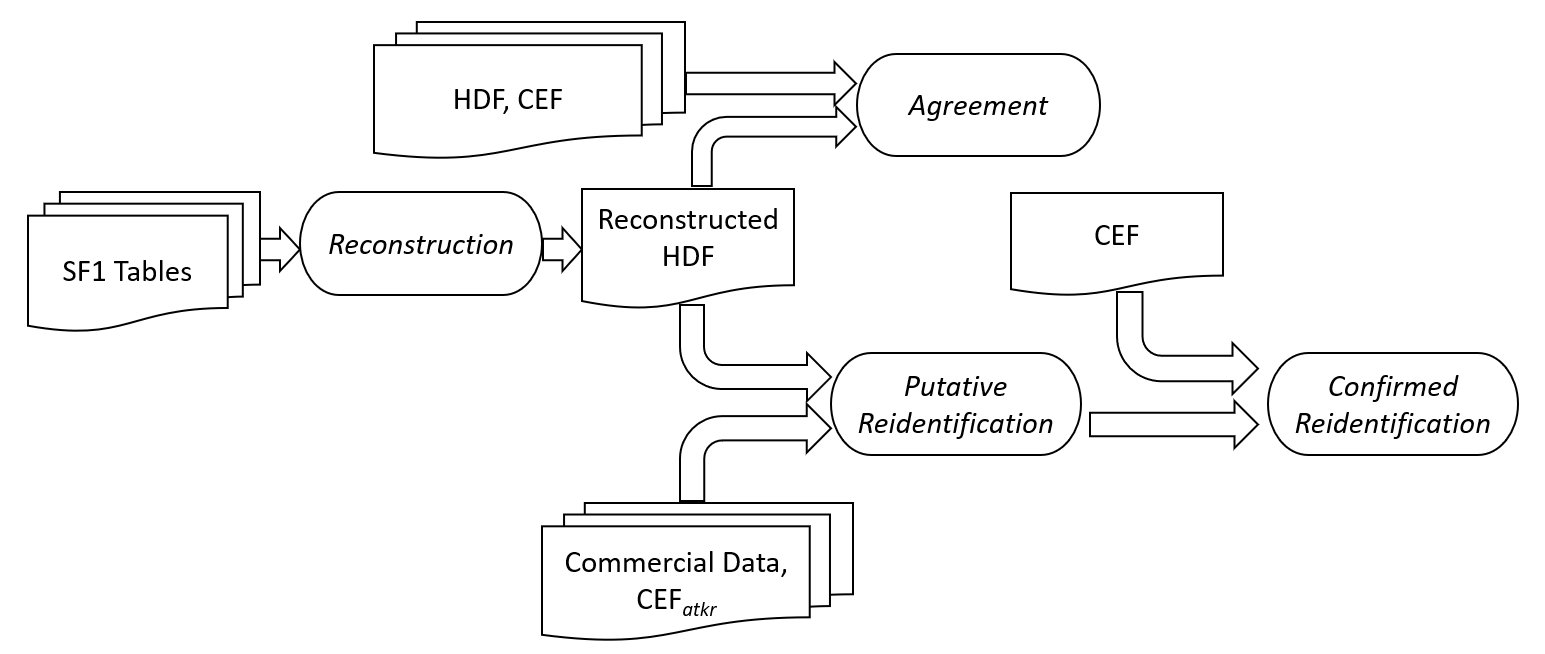
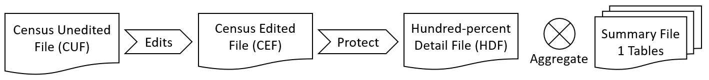
Based on Summary File 1 (SF1) tables, a database with the features and rows of the confidential Hundred-percent Detail File (HDF) is reconstructed, validated for agreement with the HDF and the confidential Census Edited File (CEF), linked to commercial databases and a quasi-identifier-only copy of the CEF (labeled ) to determine putative reidentifications, then reidentifications are confirmed by linkage to the full-feature CEF. SF1 is itself tabulated from the HDF using a processing sequence that begins with the Census Unedited File (CUF). See Figure 2.
Figure 1 provides a high-level overview of the databases that underlie the confidential and published versions of the 2010 Census and also summarizes our workflow using these databases. We begin by describing the internal Census Bureau databases from which the public SF1 was created. Next, we describe SF1 itself. We also describe the attributes and limitations of the commercial databases used in the analysis. We deliberately abstract from some of the complexity of these databases in order to focus on the features that are salient to our reconstruction and reidentification attacks.
| Dataset | |||||||||
| CUF | x | x | x | x | y | x | x | ||
| CEF | x | x | x | x | y | x | x | ||
| HDF | x | x | z | y | x | x | |||
| COMRCL | x | x | x | x | y | ||||
| x | x | x | x | y | |||||
| x | x | z | y | x | x | ||||
| x | x | x | x | x | |||||
| Putative | x | x | x | z | y | x | x | ||
| Putative | x | x | x | x | x | x | |||
| Confirmed | x | x | x | z | y | x | x | ||
| Confirmed | x | x | x | x | x | x | |||
| MDG | x | x | x | z | y | g | g | ||
| PRG | x | x | x | z | y | h | h | ||
| MDF | x | x | z | y | x | x | |||
| x | x | z | y | x | x | ||||
| x | x | z | y | x | x | ||||
| x | x | z | y | x | x |
3.2. 2010 Census internal databases
The U.S. Constitution mandates a census of population conducted every ten years. Since the 1970 Census, these enumerations have collected primarily self-reported information on households and the individuals in those households. For the 2010 Census, the confidential respondent microdata were stored in several databases. For our purposes, describing the relevant feature sets and provenance requires starting with the 2010 Census Unedited File (CUF), which contains the raw census responses for all living quarters, unduplicated and deemed in-scope for the enumeration. The 2010 Census Edited File (CEF) constitutes the final, fully edited, permanent electronic record of these responses to the 2010 Census. The application of confidentiality protections and tabulation recodes to the CEF produces the Hundred-percent Detail File (HDF), which is used to create all published data products. The tabulation edits in HDF recode the residential location to the 2010 Census tabulation geography, create various age groupings, and create a variety of race and ethnicity groupings, all described below.
As part of the internal confidentiality safeguards, the respondent’s name and address are stored on the CUF, not the CEF. Census data processing links the physical address to an identifier called the Master Address File Identifier (MAFID) that the Census Bureau’s Geography Division has determined to be a living quarter that existed on April 1, 2010, as either a housing unit or an occupied group quarters facility, and thus is in-scope for data collection in the 2010 Census. To facilitate research while safeguarding the name and address, the Census Bureau creates a crosswalk that relates the internal person-record identifier on the CEF to a person identifier called a Protected Identification Key (pik) using the production household data record-linkage system called the Person Identification Validation System (PVS).444The PVS has evolved over time. The application of the production record linkage system was completed contemporaneously with the 2010 Census data processing using the 2010-vintage version of the PVS. For details on pik assignment, see [carra-2014-01]. While the feature sets for the full hierarchical CUF, CEF and HDF are much larger, the portions of the CUF that we use are shown in Table 1 in the row labeled “CUF.”
The use of the Census Bureau’s production record-linkage system, and the selection of the 2010 Census vintage allowed us to do record linkage on name and address without having to design our own linkage system. We ensured that the same vintage of PVS was used for the commercial data we discuss later in this section. If the PVS recognized a person in the 2010 Census, it is extremely likely that the same vintage of the software would recognize the same person in the commercial data, thus assigning the same pik. All record linkage systems are subject to false positive and negative linkages. By employing the same production PVS system on all data used for this paper, we accept linkages based on piks with the error properties described in [carra-2014-02].
Not all records in the CEF have a pik and in some cases the same pik appears on multiple records because the PVS was not designed to unduplicate the input data set. For the purposes of this paper, we refer to the subset of records in the CEF with a distinct pik within the record’s census block as the data-defined population. To create the data-defined population, if there were multiple records with the same pik within a census block, one record was randomly chosen. The data-defined population is 276,000,000 records ( of all records in the CEF). Records with duplicate piks within a single block appeared in 15% of blocks. In total, 1% of records with a pik were removed by this unduplication. The remainder of the difference between the total 2010 Census population and the data-defined population are incomplete or imputed census responses to which the PVS cannot assign a pik because the CUF contained insufficient respondent-supplied data.
The MAFID is further geocoded into the 2010 Census tabulation geography. In this paper, we distinguish two components of the 15-digit tabulation geography–census tract (11-digit concatenation of FIPS state, county equivalent, tract) and census block (15-digit concatenation of FIPS state, county equivalent, tract, block).555FIPS stands for Federal Information Processing Standards, and refers to numeric and two-letter alphabetic codes defined in U.S. FIPS Publication 5-2. FIPS 5-2 was superseded by ANSI standard INCITS 38:2009. For details, see [ansifips]. Census blocks are a statistical definition of geography, not the commonly used “city block,” with complete coverage of the entire territory of the United States, and are the atoms in the Census Bureau’s geographic lattice that are used to build all other geographic tabulation summary levels, such as census tracts or county equivalents. Census blocks are defined in terms of territory, not population, and tessellate the entire United States. Some blocks may therefore be uninhabited (even underwater), others may have a very large population. See [censusblocks] for an overview. For more details on the person and geography attributes, see [sf1:2010:tech]. The HDF is formed from the CEF by applying the SDL methods described in Section 2.2, which are called “confidentiality edits” in the technical documentation [sf1:2010:tech]. Finally, the parts of the person records in CEF and HDF used in this paper have the feature sets shown in Table 1 in the appropriately labeled rows.
The confidential databases share the same schema and feature sets: one column for the census block, one column each for the person identifier (pik), sex, age, and ethnicity (Hispanic or Lation/Not Hispanic or Latino), and six columns for the required race categories.666For details on the person attributes, see [sf1:2010:tech]. For background on the definitions of the required race and ethnicity categories, see Statistical Policy Directive 15 [OMB:1997]. The category “some other race” is mandated by law, not statistical policy. Persons may self-declare multiple race categories; hence the binary race features are not mutually exclusive. In practice, most 2010 Census respondents only identified with a single race. The feature age is recorded in integer values. If a census response is missing, the process that creates the CEF performs edits and imputation, called “allocation” in the technical documents. There are no missing data in the CEF and, in particular, at least one of the six race categories must be selected. Excluding pik, which is standing in for name, we define all valid combinations of block, sex, age, race, and ethnicity as the feature space (sample space in statistics) for CEF and HDF, . There are approximately (161 billion) such combinations which gives the cardinality .777 Cardinality , where is the number of inhabited blocks in the 2010 Census, 103 is the number of single-year age categories 0 to 99 plus grouped ages 100-104, 105-109, 110+ allowed in the published tables, and is the number of allowable race combinations. Note that, for technical reasons, when we implement the reconstructions of HDF, we modify the feature set to eliminate the age binning for ages 100+. Finally, note that we used data for the 50 states and the District of Columbia.888The use of the term “state” in this document refers to all 51 state-equivalent political divisions. We excluded Puerto Rico because the 2010 vintage of the Census Bureau’s production name and address record linkage system did not work as well for this commonwealth.
3.3. 2010 Summary File 1
The most extensive and widely used 2010 Census data product is Summary File 1 [sf1:2010:tech]. Figure 2 illustrates the process of creating SF1 from the internal census databases. SF1 contains counts of persons, households, families within households, group quarters residents, and housing units tabulated at the census block, census tract, and county-equivalent geographic levels. SF1 also includes the tables released separately as the 2010 P.L. 94-171 Redistricting Data Summary File, which forms the basis for redistricting every legislative body in the United States and is normally released by March 31st of the year following the decennial census, several months before SF1.999The populations used for apportionment include a limited number of U.S. citizens and their families living abroad, known as the Federally Affiliated Overseas Population. These persons do not have records in the CEF, and their total for each state is added to the residential population for that state prior to apportionment, see Appendix G of [sf1:2010:tech]. The P.L. 94-171 Redistricting Data Summary File tables are renumbered in SF1 but are otherwise identical to the original release.
The SF1 and other published tables are created by tabulating the HDF according to various combinations of geographic and demographic detail. All published data from the 2010 Census used the same geographic hierarchy. See Appendix A of [sf1:2010:tech] for more details. The census block is the most detailed geographic category. There were 11,078,297 blocks defined for 2010 Census publications of which 6,207,027 had nonzero populations.101010Whether a block was inhabited or not was published without any confidentiality edits in 2010. These census blocks aggregate into 73,057 defined census tracts of which 72,531 had nonzero populations. These census tracts, in turn, aggregate into 3,143 county equivalents, all of which had nonzero populations.
Within this hierarchy, tables of varying demographic and household detail are created. In this paper, we focus on block- and tract-level tabular summaries of persons using only the 34 tables shown in Table 2. The census block-level tables, labeled in Panel A of Table 2, provide detailed information on sex and race, but with coarsened age information for those age 22 and over. The census tract-level summaries, labeled in Panel B of Table 2, report most of the detail in block-level tables in addition to reporting more detailed age.111111The tract-level schema for race is less detailed than the block-level schema; however this does not affect our reconstructions because we never use the tract-level data alone, and its race and ethnicity schema is nested in the block-level schema. We note for completeness that the 2010 Census PUMS, Summary File 2, and the American Indian/Alaska Native Summary File were also created from the HDF. The 2010 HDF itself, but not the 2010 CEF, can be used by external researchers with approved projects in the Federal Statistical Research Data Centers.
| Panel A: Tabulated at the Census Block Level | |||||||
| P1 | P6 | P7 | P8 | P9 | P10 | P11 | P12 |
| P14 | P12A | P12B | P12C | P12D | P12E | P12F | P12G |
| P12H | P12I | ||||||
| Panel B: Tabulated at the Census Tract Level | |||||||
| PCT12 | PCT12A | PCT12B | PCT12C | PCT12D | PCT12E | PCT12F | PCT12G |
| PCT12H | PCT12I | PCT12J | PCT12K | PCT12L | PCT12M | PCT12N | PCT12O |
3.4. The Treatment of Age in Summary File 1
2010 SF1 tabulated age differently depending on the specific table and the level of geographic detail. At the tract level and above (e.g., Table PCT12), age was tabulated in single years from 0 to 99 years, then binned into the ranges 100-104 years, 105-109 years, and 110 years and over. At the block level in most tables (e.g., Table P12), age was binned into the following ranges: 0-4; 5-9; 10-14; 15-17; 18-19; 20; 21; 22-24; 25-29; 30-34; 35-39; 40-44; 45-49; 50-54; 55-59; 60-61; 62-64; 65-66; 67-69; 70-74; 75-79; 80-84; and 85+. Also at the block level, Tables P10 and P11 selected only persons age 18 and older. Finally, the block-level table P14 selected only individuals age 20 or younger and encoded age in single years. Combining the different age binning and universe selection rules applied at the census block level defines the most detailed age schema that these tables can support. That schema has 38 age groups: single year of age from 0 to 21, then: 22-24; 25-29; 30-34; 35-39; 40-44; 45-49; 50-54; 55-59; 60-61; 62-64; 65-66; 67-69; 70-74; 75-79; 80-84; and 85+. We use this 38-bin age schema (feature agebin) in our assessments of agreement of the reconstructed HDF with the HDF and CEF. We show in the reidentification experiments that the 38-bin age schema provides sufficient uniqueness for persons at the census block level to enable reconstruction-abetted reidentification. It is important to note that tables P12 and P14, when combined, give the exact number of males and females in each of the 38 age bins in each census block, so any remaining uncertainty is in the race and ethnicity distribution within each sex and age bin. For any reconstructed microdata based on at least the tables in Panel A of Table 2, there is only one possible reconstruction on the feature set {block, sex, agebin}; that is, the reconstruction is exact on that feature set. In our matching algorithms, we distinguish between matches based on exact age (feature age) and those based on binned age (feature agebin). In Section 4.5 we elaborate on the solution variability of our reconstructions.
3.5. Circa 2010 Commercial Databases
We created the commercial data (COMRCL) used for our reidentification experiments by combining data extracts originally purchased in support of the 2010 Census evaluations from four commercial providers between 2009 and 2011.121212The four commercial databases were provided by Experian Marketing Solutions Incorporated, Infogroup Incorporated, Targus Information Corporation, and VSGI LLC. The databases used are the same as in [rastogi2012] except that we excluded data provided by the Melissa Data Corporation, which contain address information but not sex and age data. The COMCRL data serve as the background knowledge of an attacker with low-quality information contemporaneous with the release of the 2010 SF1. While the database schema and the purposes for which these commercial databases were originally collected vary, they all share certain attributes. All have basic personal identifying information (PII) including names, addresses, sex, and birthdates. The vintage 2010 versions of these databases that we used did not include self-reported race and ethnicity data.131313Race and ethnicity data are modeled in some of the commercial databases [rastogi2012].
We harmonized the feature sets for the commercial data to match the schemas used in the CEF, as indicated in the COMCRL row of Table 1. These data were originally acquired because the features we use—name, address, sex, and birthdate in particular—were expected to closely resemble those collected on the 2010 Census. In our harmonization, name and address were mapped to pik and MAFID, respectively. The MAFIDs were originally geocoded in 2009-2011, when these commercial databases were acquired. Because the final 2010 tabulation geography schema was not available at that time, we remapped the MAFID to final 2010 tabulation blocks in early 2019. PII was standardized and mapped to pik using the same 2010-vintage PVS that was used for the 2010 CUF. Table 3 shows that there were 289,100,000 records with a valid pik, block, sex, age in the commercial database. We excluded the 2,449,000 COMCRL records that have census block IDs outside the 2010 CEF universe from all reidentification studies using COMCRL. Among the COMCRL records in the CEF universe, only 106,300,000 () matched a CEF record on pik, block, sex, agebin, i.e., using binned age instead of exact age. Because our experiments on vulnerable populations—those whose characteristics differ from the modal person—use the census block universe for the {race, ethnicity} features to define vulnerable populations, only the 106,300,000 COMCRL records that match CEF records on the feature set {pik, block} are available for those studies. Thus, the commercial data used here are not very accurate compared to the 2010 CEF, and we do not rule out the possibility that better quality data may have been available in 2010. Better external data were available for the 2020 Census [brown:etal:2023].
| In CEF Universe | Not in CEF | |||
| Matched | Unmatched | Universe | Total | |
| () | () | () | () | |
| Records in COMRCL | 106,300 | 180,400 | 2,449 | 289,100 |
| Records not in COMRCL | 169,700 | |||
| Total | 276,000 | |||
4. Reconstruction Methodology
We define database reconstruction as any attempt to re-create the record-level image of the database from which a set of published query results or tabulations were originally calculated; in this case, that is the confidential HDF.141414See [garfinkel2018a] for a longer discussion of how to understand database reconstruction. Database reconstruction attempts to reverse-engineer the confidential HDF records that were the input data used in a tabulation system with the goal of making the reconstruction as close as possible to these confidential data. We note that the reconstruction described here is not the most powerful feasible reconstruction. We used only a subset of the SF1 tables, we made no attempt to reconstruct households or characteristics of the householder (adult respondent providing the census data on CUF), and we did not use statistical modeling to improve the reconstruction (e.g., in blocks where multiple different reconstructions were consistent with the published tables, we did not use statistical methods to identify the most likely reconstruction). Even without these enhancements, we show that the disclosure avoidance methods of the 2010 Census are highly susceptible to attack.
4.1. Reconstruction Overview
Table 2 shows the 34 tables we included in our reconstruction for any universe that was part of the total population.151515We did not use tables where the universe was households, which means that we did not use the “relationship to the householder” information to reconstruct household characteristics or to improve the reconstructed data for persons in those households. These tables, computed from the HDF person records, are multidimensional marginal counts related to sex, age, race, and ethnicity by census block and tract. Our reconstructed microdata contain these same variables and only these variables. The reconstructed data, therefore, necessarily reflect the schemas used for SF1 and are only informative about variables, in particular age, in the schemas used for publication, as described in Section 3.4.
Our experiments use two different subsets of SF1 data as shown in Table 2. The first reconstruction, which we denote as , uses both tract and block-level SF1 tables, taking advantage of both the geographic and race detail in the block summaries and the age detail in the tract summaries. The second reconstruction, , uses only the block-level tables. Thus, the second reconstruction removes the more granular age information found in the tract-level tables while retaining the full race and ethnicity schema used in the block-level data. Comparing results from and to HDF and CEF shows the loss of reconstruction accuracy from removing tract-level tables.
4.2. A Simplified Algebraic Representation of the Reconstruction Problem
Because it is very useful for understanding the mathematical structure of the reconstruction experiments, we begin by explaining the linear algebra representation of the reconstruction problem. Then, in Section 4.3, we provide a description of the integer program (IP) setup we used to generate the solutions discussed in our results. This IP formulation does not convey the high-level structure of the problem as simply but closely follows our software implementation.
The inputs to the reconstruction are the database schema for the tabulation feature set {block, sex, age, race, ethnicity}; the vector of all published statistics in the appropriate order; and the matrix workload that maps the histogram representation of the HDF onto the published statistics. We represent the table of the record-level data as the vectorized fully saturated contingency table (called a histogram in computer science) where every cell corresponds to a possible record type in and its value is the number of records of that type. Thus, instead of a multi-dimensional array, the contingency table is flattened into a vector (like the operation as.vector() in R or np.flatten() in numpy). Let represent the contingency table vector. Database reconstruction consists of finding at least one non-negative integer solution for in the equation system
| (1) |
where is column vector of the statistics extracted from SF1 for a given reconstruction, is the matrix for computing those SF1 tabulations from a contingency table vector , and is the set of non-negative integers. Each row of and corresponding component of , therefore, represent the formula for a single statistic and its realized value in SF1, respectively.
There are fewer statistics published per block than points in the sample space (), meaning that a unique solution to equation (1) is not always guaranteed. However, many low-population blocks have published tables that contain a large number of entries whose values are zero. This eliminates many candidate solutions, and often there is only one unique non-negative, integer-valued solution to equation (1). There is always at least one solution because SF1 was tabulated from a single real database with the schema encoded in (i.e., the HDF). The commercial software GurobiTM has a robust toolkit for solving IPs and related mixed integer linear programs (MILP) to produce solutions to problems such as these. See Section 4.3 for details. When multiple solutions exist, GurobiTM will pick one. In principle, statistical modeling could be used to select among candidate solutions to improve reconstruction quality, but we did not do this.
Given a solution to equation (1), another question of interest is how different could be from other possible solutions. If is the only solution to equation (1), then it represents an exact reconstruction of the microdata used to tabulate SF1, namely HDF, with certainty. Moreover, if the uniqueness of the solution can be determined from the published inputs to equation (1), then an attacker knows that those reconstructed records were present in HDF with certainty. To examine how often the solution was strongly constrained, we designed an algorithm for measuring solution variability by building a second IP model. Its goal is to find a second solution, , that maximizes the distance to . This allows an attacker, using only public information, to determine the maximum number of records in the reconstruction that could be incorrect. This problem is described in Section 4.5.
4.3. The Integer Programming Version of the Reconstruction Model
This section describes how the IP is implemented as a mathematical programming problem, which is the method used in all our statistical calculations. We begin by describing how we converted the basic schema for the feature set {block, sex, age, race, ethnicity} into the binary variables used in our reconstruction. The following notation describes the nine demographic features: W, BL, AIAN, ASIAN, NHOPI, SOR, HISP, SEX, and AGE and the values allowed for each feature.
| (2) | Reconstruction Feature Sets Using Exact Age | |||
| W | ||||
| BL | ||||
| AIAN | ||||
| ASIAN | ||||
| NHOPI | ||||
| SOR | ||||
| HISP | ||||
| SEX | ||||
| AGE | ||||
A potential record corresponds to a setting of the block along with settings for the demographic attributes (w, bl, aian, asian, nhopi, sor, hisp, a, s). Here the lowercase italic letters index the permitted values of the uppercase feature set of the same name (e.g. represents a value of the feature AIAN). We create one variable for the IP for each potential record. Since we do not know, a priori, how many records exist with the same demographic type and block, we must create multiple variables for . We use Table P12 from SF1 (age group by sex for each census block) to obtain an upper bound on the index for each block and combination of demographics. For example, for the demographic type of a 22-year-old Asian Hispanic female in a block , suppose Table P12 for that block indicates that there are 50 females in the age group 22-24 (See Table 4 for the age groupings in P12). This is an upper bound on the number of potential records for 22-year-old Asian Hispanic females in the block. Thus, we create the 50 variables for . These variables are binary, with a value of 1 indicating the presence of the potential record in a candidate microdata reconstruction. Once the binary variables are assigned values, the summation
represents the number of 22-year-old female Asian Hispanic people in that block. Formally, we created the complete set of binary variables as follows.
- •
-
•
For any age , sex , and block , define the constant to be the count in SF1 Table P12 of the number of people in block with sex and an age that is in the same age bin as age .
-
•
For every block , age , sex , and value of the race/ethnicity variables w, bl, aian, asian, nhopi, sor, hisp, we define the binary variables:
(3)
We emphasize that using SF1 Table P12 in this manner does not coarsen the age schema. It only determines the maximum number of variables that the integer program may use for each demographic type in the full schema.
| a | 0-4 | 5-9 | 10-14 | 15-17 | 18-19 | 20 | 21 | 22-24 | 25-29 | 30-34 | 35-39 |
| z | 0 | 1 | 2 | 3 | 4 | 5 | 6 | 7 | 8 | 9 | 10 |
| a | 40-44 | 45-49 | 50-54 | 55-59 | 60-61 | 62-64 | 65-66 | 67-69 | 70-74 | 75-79 | 80-84 |
| z | 11 | 12 | 13 | 14 | 15 | 16 | 17 | 18 | 19 | 20 | 21 |
| a | 85-110 | ||||||||||
| z | 22 |
Let T represent the set of all census tract indices, and represent the set of all census block indices in tract . We next illustrate how each SF1 table adds additional constraints on the variables. For example, consider the tract-level table PCT12I, which encodes the tabulation sex by age group in each tract for people who are “White Alone” and “Not Hispanic or Latino.” The age binning used by this table is , so let AGEBINPCT12I be the function that returns the appropriate PCT12I age bin for a given age . For each tract , PCT12I age bin , and sex , let be the corresponding count in table PCT12I. Then for each we add the following constraint:
where the summation over uses the upper bound on the number of variables in equation (3) (i.e., ).
| a | 0 | 1 | 2 | 3 | 4 | 5 | 6 | 7 | 8 | 9 | 10 |
| z | 0 | 1 | 2 | 3 | 4 | 5 | 6 | 7 | 8 | 9 | 10 |
| a | 11 | 12 | 13 | 14 | 15 | 16 | 17 | 18 | 19 | 20 | 21 |
| z | 11 | 12 | 13 | 14 | 15 | 16 | 17 | 18 | 19 | 20 | 21 |
| a | 22-24 | 25-29 | 30-34 | 35-39 | 40-44 | 45-49 | 50-54 | 55-59 | 60-61 | 62-64 | 65-66 |
| z | 22 | 23 | 24 | 25 | 26 | 27 | 28 | 29 | 30 | 31 | 32 |
| a | 67-69 | 70-74 | 75-79 | 80-84 | 85-110 | ||||||
| z | 33 | 34 | 35 | 36 | 37 |
We use the notational shorthand to represent all such constraints created by SF1 tract-level table (e.g., PCT12I) for tract . Specifically, the notation refers to the optimization variables for records in a block when performing the reconstruction, the notation indicates that we form the constraints using the optimization variables for all blocks that belong inside tract (i.e., ). For example, in the case of SF1 Table PCT12I, this means an application of equation (4.3) for each age bin and sex for the record variables in the tract. The tract-level tables used are listed in Panel B of Table 2. Similarly, we use the shorthand for the block-level constraints in block created by SF1 block-level table (Panel A of Table 2).
With this notation, the IP problem for the reconstruction model for tract can be written as:
| (4) | ||||
The objective function “max 0” indicates that any feasible solution that satisfies the constraints can be returned (i.e., if there are multiple candidate solutions, no statistical modeling or maximum entropy is used, and GurobiTM picks a solution arbitrarily). The optimization variables are the defined in equation (3). Once we have a feasible solution, for every that is set to 1, we add a corresponding record for that block and demographic type to the reconstructed dataset. For , we also recode the feature age into agebin because our matching algorithms require access to both variables. See Section 5. Thus, upon completion, the IP from equation (4) yields a reconstructed version of the HDF, called , that contains one record for each person in the 2010 Census with the features indicated in row of Table 1.161616 Since SF1 always groups all persons 100 years of age or older into the bins: “100-104 years”, “105-109 years”, and “110 years and over” or uses even coarser age groups, the IP can never resolve the feature age more precisely than these bins. The IP still has variables for individual ages 100, …, 110 and so Gurobi will arbitrarily choose a specific age within those age bins. This means that there is inherent solution variability in the ages of the oldest sub-populations.
Next, we present the IP for the reconstruction , which uses only the SF1 block-level tables shown in Panel A of Table 2. Block-level tables use several age binning schemes, but their intersection is not exact age. Instead, their intersection is the age grouping shown in Table 5, which has 38 age bins. Since this is the most fine-grained age resolution that can possibly be obtained from block-level tables, contains age reconstructed up to this 38-age binning (the feature that represents this age grouping is called agebin). To simplify the implementation, the IP uses the optimization variables from equation (3). This means that the solution provides single-year ages, but after the reconstructed microdata are created, we recode age into agebin as defined in Table 5. The IP for the block-level reconstruction is similar to the tract-level reconstruction. For each block , solve
| (5) | ||||
Again, no statistical modeling is used to return the most plausible solution if multiple feasible solutions exist. Once we obtain a feasible solution, for every that is set to 1, a corresponding record for that block and demographic type is created. Because our matching algorithm requires access to both age-related features, we retain the feature age and create the feature agebin using the appropriate bin in Table 5. The resulting record is added to the reconstructed dataset whose feature set is shown in the row of Table 1.
4.4. Implementation Notes
The IP formulation of the reconstruction problem is mathematically equivalent to the simplified model in Section 4.1. The only difference is that the optimization variables in the IP implemented in our code correspond to potential records, while the vector in equation (1) contains counts from the fully saturated contingency table defined on the sample space . The code in the replication archive implements the IP in equations (4) and (5), and these equations are useful for reading the software implementation in the replication archive, whereas the histogram representation in equation (1) is useful for understanding the high-level structure of the problem. For reconstruction outcomes, only run-time, not the space of feasible solutions, is affected by the choice of which representation to implement. It is not obvious a priori which representation should solve more quickly. We have direct experience solving the IP representation, and we found it to consistently solve very quickly at default GurobiTM settings for the set of tables we used in the reconstruction. Equation (1) is succinct, easy to represent in any matrix programming language that implements sparse matrix storage and MILP solvers, and yields a model with considerably fewer variables. On the other hand, the IP representation, while it produces less succinct models, uses only binary variables in the solution set, rather than non-negative integers, and binary variables are usually processed more efficiently in modern MILP solvers. Our discussion switches between the two representations to permit clarity of expression (equation (1)) versus fidelity to the details of our implemented reconstruction code (equations (4) and (5)).
4.5. Solution Variability
When an attacker performs a reconstruction, an important question is whether the attacker can determine if the reconstruction in a block is unique, or if the attacker can compute an upper bound on the number of reconstructed records that may be erroneous (i.e., a confidence score for reconstruction accuracy). In blocks with zero reconstruction error, an attacker would also be more confident about linking these reconstructed records to other data sources, since swapping and record-level synthetic data would be the only remaining disclosure avoidance techniques that could cause these reconstructed HDF records to differ from their CEF counterparts. This would be especially problematic if the swap rate were low. On the other hand, a high swap rate may prevent some records from being linked, but for the remainder of the records that are linked (and hence probably not swapped), the attacker would be more likely to learn additional attributes about those individuals from the reconstructed data. Recall that reconstruction error is limited to the race and ethnicity variables, along with the specific age within agebin. As explained in Section 3.4, SF1 tables P12 and P14 already give the exact count of males and females in each of the 38 age bins from the block-level schema for each block. This means that an attacker can always create microdata records with the correct sex and binned age values by expanding those tables. In the agebin schema, the only remaining uncertainty is in which race and ethnicity to attach to those records. In the tract-level age schema, there is also uncertainty about single year of age within age bin except for the population 21 years and under, since each of these age bins contains exactly one age.
For any reconstruction rHDF and geographic region , such as a specific tract or block, we let represent the subset of records in rHDF that belong to geographic region . If there are two feasible reconstructions, and , we consider them equivalent for region if and only if the difference is the ordering of the records; that is, if one is a permutation of the other. In other words, two reconstructions are equivalent on if their corresponding fully saturated contingency tables for region are the same. Letting represent the operator that converts a reconstruction into a fully saturated contingency table, two possible reconstructions and in region are distinct whenever .
Let index the cells of the histogram representation of the contingency table. We measure the difference between two histograms using the norm:
Note that the cells depend on the reconstruction schema. For example, when measuring solution variability relative to the agebin feature, the histograms use the 38-bin age grouping shown in Table 5. Also note that
where is the total population of geographic unit . Equality is achieved if and only if the two histograms completely disagree on the types of records present in . This bound follows because and are both constrained to have exactly records, so we can think of as being constructed by modifying a sequence of records in . Each such modification can increase the distance by no more than 2, and at most every one of the records can be modified, for a total distance of when the two histograms no longer have any records in common. On the other hand, the norm is 0 if and only if the two histograms agree exactly on the types and multiplicities of records present.
Given a feasible solution , we define solution variability relative to as the following function for geographic unit :
| (6) |
where feasible solutions use equation (4) when is a tract or equation (5) when is a block. Note that the multiplication by 100 allows us to interpret as the percentage of its maximum value.
If solution variability in equation (6) is 0, then there is a single, unique solution to the reconstruction problem in geounit , and the records in must exactly match the HDF for the variables present in records of both data sets and under the schema used to create . When solution variability in equation (6) is 100, there is at least one other reconstruction that has no records in common with . In this case, may be a poor reconstruction of HDF, and any agreement between the two may be due to happenstance. In general, is an upper bound on the percentage of records in that could differ from any other possible reconstruction, including the actual HDF. For example, if the solution variability is 10, then at most one-tenth of the records (i.e., 10%) in could differ from the actual HDF. Note that “differ” means that at least one attribute of the record is incorrect; it does not necessarily mean all attributes in the record were wrong.
It is worth noting that solution variability is a property specific to a given reconstruction because it measures the maximum percentage of records of that can be changed while still maintaining a feasible reconstruction. Thus two different reconstructions and can have different solution variabilities. For instance, suppose is in the middle of the feasible region and is in a remote corner of the feasible region. Then, the solution variability of is less than that of .
Given that an attacker may use a different solver or statistical modeling to find a feasible reconstruction, it is important for the data curator to understand the range of solution variability any attacker may obtain. Fortunately, using our method, the data curator can estimate a 100% confidence interval that is guaranteed to contain the attacker’s solvar value. To do so, the data curator obtains a reconstruction , computes its solution variability for a region , and appeals to the triangle inequality as follows. For any other feasible ,
| (7) |
and hence any attacker’s solvar will be within a factor of 2 of the data curator’s solvar.171717These bounds also address a technical caveat which is appropriate for our implementation: as an engineering quirk, the process we followed to produce the solution variability estimates involved re-solving the initial reconstruction optimization problems, not directly re-loading the original reconstruction solutions used for the initial reconstruction-abetted re-identification attack. The GurobiTM software that we used for reconstruction is largely, but not completely, deterministic at default settings. This nondeterminism could have caused the used in solution variability problems to differ from the original reconstructed solutions in some cases, although we suspect this would be unusual.
Computing for each block is manageable using GurobiTM, but computing solvar for larger regions can be very computationally expensive. Let denote the set of blocks composing region and, as usual, and refer to the population counts in block and region , respecitvely. Given , for each , we define cumulative solution variability, cumsolvar, as:
| (8) |
Recalling that is the set of all the blocks in tract , , is an upper bound on the percentage of records in tract for which any two solutions to can differ.181818The analogous claim is not true for , because our solution variability models, described in equations (9) and (10), make use of some tract-level tabulations. By removing tract-level tabulations, is less constrained and so has a larger feasible region. The function cumsolvar is of particular interest for regions composed of all blocks with no greater than the percentile for different values of (see Table 6). In particular, we focus our attention on persons who live in the set of blocks with . For these blocks, we know that the attacker is certain that the reconstructed records are in HDF regardless of the method used to compute the reconstruction.
4.6. Solvar Implementation Details
The integer program that determines solution variability in geography is computationally more expensive to solve than solving for an initial . For an attacker who wants to target a small number of blocks or tracts, that is not much of an issue. However, the data curator needs to compute the solution variability for all block and tracts. We found that computing a solution to equation (6), in which the feasible is required to be consistent with the block and tract level tables, is too expensive to perform for the entire nation. Hence, we relaxed the optimization problem to make it easier to solve while still allowing us to bound the solution variability for an attacker who performs a reconstruction using block and tract-level tables. While concerted research on this problem class is likely to yield faster solutions, we found that the following changes made the problem easier to solve. First, we use the 38-bin age groupings (feature agebin) that appear in the block-level tables.
Next, we change the starting solution, , around which solvar is computed by relaxing the tract-level constraints that define a feasible solution from equality constraints to inequality constraints. For a given block and its containing tract , we solve the following optimization problem:
| (9) | ||||
| s.t. | ||||
The differences from the reconstruction in equation (4) are that equality constraints for tract-level tables become inequality constraints, and the other blocks in tract are ignored when computing a reconstruction for block . Specifically, only optimization variables for block are used when forming the tract-level constraints, hence the left-hand side of the tract-level constraint is an underestimate of the counts in the tract-level tables.
Once we have for a block , we search for the that is furthest from while satisfying the same constraints. Specifically, for a given corresponding to block in tract , we solved the following IP:
| (10) | ||||
| s.t. | ||||
Note that the tract-level tables in the solvar equation (10) appear in inequality constraints. Variables for records in other blocks within the same tract do not appear in this optimization problem for block .
We note that the IP for the initial solution for is a strict relaxation of the constraints used for the reconstruction solving equation (4). This implies that the feasible region for is a superset of the feasible region for . Similarly, the solvar IP in equation (10) also searches for from a strictly larger solution space. This property implies that upper-bounds the solvar value for tract that an attacker would get using the stronger tract-level constraints. In other words, , , upper-bounds the percentage of records by which any two solutions to can differ because first, the union is a solution to a problem with a strictly larger solution space than , and second, upper-bounds the percentage of records by which any two solutions to this problem can disagree.
The problem relaxations we performed probably made our upper bound on solution variability much looser. Hence, strengthened (and even more concerning) solution variability bounds may be produced in the future. However, since summing the block-level solution to equation (10) and multiplying by 2 is also an upper bound on the exact solution variability for the tract-level problem, the large number of blocks with 0 block-level solution variability will still contribute 0 to the tract-level solution variability in the schema. Thus, the variability in these blocks is already bounded by 0 and cannot get tighter. Tracts with 0 tract-level solution variability found in solving the optimization problem (10) must also have 0 solution variability in any stronger tract-level IP.
We found that solution variability could be readily computed using the optimization in equation (10) for all 6,207,027 blocks with positive population in the 2010 Census tabulations. This demonstrates that attackers have a public, computationally feasible method for independently identifying blocks for which aggregation into tables introduces no additional uncertainty about the underlying microdata beyond the SDL measures that were applied at the record level to generate the HDF. No access to confidential data is required to perform these solution variability calculations. Furthermore, population uniques found in blocks with 0 solution variability are provably population uniques in the HDF, again without using any confidential data. And population uniques using the feature are provably population uniques on the exact age feature. Finally, incorporating additional SF1 tables to the ones shown in Table 2 can only decrease solution variability. Since we used only 18 of the 177 census block-level tables and 16 of the 84 census tract-level tables, our solutions to equation (10) are also upper bounds on the solution variability of reconstructions that use additional tables.
5. Matching and Reidentification Methodology
To assess the quality of the reconstructed microdata and execute the reidentification experiments we perform several different types of matching between various data sources. Referring again to Figure 1, we now discuss the methodology employed to compute agreement between the reconstructed and confidential data and to measure the success of our reidentification experiments using those reconstructions.
For either or , our first-order assessment of the quality of the reconstructed microdata matches these reconstructions directly to both the HDF and CEF. This is not a record linkage assessment. It compares the reconstructed microdata directly to the source microdata for the contingency tables in SF1, namely HDF, and to the source microdata for HDF, namely CEF. We label this step the agreement match because it provides measures of agreement in record-level feature values between or and the confidential HDF and CEF. After the agreement match, we do record-linkage based reidentifcation matches to see how accurately an attacker can infer race and ethnicity from the reconstructed microdata. Thus, we link and separately to both commercial data and a specially constructed extract from the CEF called that includes linking variables (quasi-identifiers) from the schema in equation (2) and the person identifier pik but no other variables—specifically, not race or ethnicity. These feature sets are shown in the rows COMCRL and on Table 1.
By record-linkage of the quasi-identifiers {block, sex, (age or agebin)} in reconstructed microdata to attacker databases that include names (feature pik), we create putative reidentifications. To enhance the attacker’s database, we attach the data on {race, ethnicity} found on or to the {pik, block, sex, (age or agebin)} information in the attacker’s database—either COMCRL or . The feature sets for the records in these putative reidentification databases are shown in the rows labeled Putative and Putative in Table 1. Finally, to evaluate the accuracy of the putative reidentifications, and classify confirmed reidentifications, we match putative reidentifications to the full CEF, linking on {pik, block, sex, (age or agebin)} and comparing the {race, ethnicity} inferred from the reconstructed microdata (attached to a putatively reidentified person) to that person’s actual census responses in the CEF. We label the reidentification confirmed, when {pik, block, sex, (age or agebin), race, ethnicity} all match in either the schema in equation (2) for the feature age or the schema in Table 5 for the feature agebin. The feature sets for these confirmed reidentifications are shown in the rows labeled Confirmed and Confirmed in Table 1. Finally, we use the ratio of confirmed to putative identifications as the measure of precision or accuracy for the attack.
To make the meaning of this exercise as clear as possible, we state the attacker model we are simulating concisely here. The attacker is an entity external to the Census Bureau with no access to the confidential data contained in HDF or CEF. The attacker has access to all published 2010 Census data—every table in SF1, in particular. The attacker selects a subset (possibly the universe) of these tables and performs record-level reconstruction, possibly using the algorithms in this paper. The attacker also has access to an external database that contains name and address (or some other personal identifying information sufficient to tag a unique person like Social Security Number) and quasi-identifiers—features that match some of the features in SF1—specifically, census block (geocoded from address), sex, and age. Notice that we have explicitly used the same feature set definitions for the attacker’s database as we used in our reconstruction. This is an essential characteristic of a record-linkage attack—the attacker knows enough about the definitions of the feature set for SF1 to construct quasi-identifiers with the same schemas. The attacker matches the external data to the reconstructed record-level data from SF1 using the matching variables (quasi-identifiers) {block, sex, age} and adds the other variables reconstructed from SF1 to the external database. These added variables can include any feature tabulated in SF1, including those tabulated for housing units and householders because those data can be reconstructed as part of the record for “person 1” or “householder,” the individual who completed the census responses for the persons living in the housing unit. In our experiments the extra variables are {race, ethnicity}.191919Implementing additional features in the reconstructed data is outside the scope of this paper; however, it is straightforward to add the feature “relationship to householder.” We sketch the details here. See the documentation for Table P29 Household Type by Relationship [sf1:2010:tech]. Notice that the universe is “Total Population,” which implies that the marginal total in each of these block-level tables is the block population in Table P1. Create binary variables for the 20 mutually exclusive and exhaustive relationships defined in Table P29: family male householder, family female householder, spouse, biological child, adopted child, stepchild, grandchild, brother or sister, parent, parent-in-law, son-in-law or daughter-in-law, other relatives, nonrelatives, nonfamily male householder living alone, nonfamily male householder not living alone, nonfamily female householder living alone, nonfamily female householder not living alone, nonfamily nonrelatives, group quarters institutionalized person, and group quarters noninstitutionalized person. Add the statistics from Table P29 to the set in Table 2. Add the constraints implied by these tables to the IP in equations (4) and (10). To further reduce solution variability, if any, in the relationship variables and {race, ethnicity}, add Tables P29A–P29I Household Type by Relationship for major {race, ethnicity} categories. To further reduce the solution variability, if any, in the household population universe, add Table P30. To further reduce the solution variability, if any, for children add Tables P31 and P32. To further reduce the solution variability, if any, for persons ages 65 and older, add Table P34. It is not necessary to add the full variable “relationship to householder” to further reduce solution variability in the features {race, ethnicity}. Using only “lives in household” (all relationships except the last two) and “lives in group quarters” (the last two relationships), use Tables P16A–P16I Population in Households by Age for major {race, ethnicity} categories. Once the relationship “householder” has been reconstructed (all categories that contain the word householder), solution variability for the householder’s {race, ethnicity} can be further reduced by adding Tables P18A–P18I Household Type for major {race, ethnicity} categories. Many tract-level SF1 tables also contain information that can further reduce remaining solution variability.
At this point the attacker is using the information from what we call putative reidentifications as record-level variables on the external database. The attacker may not care about the quality of these putative reidentifications; however, because the solution variability in the schema of our attack is 0 for 70% of all census blocks using just the 34 tables in Table 2, the attacker may be satisfied with the 97 million persons for whom they know with certainty they have exactly the information on the confidential internal database. Alternatively, the attacker can keep adding tables from SF1 until solution variability is 0 for as large a portion of the target population as desired. For all records for which solution variability is 0, the attacker knows with certainty that the data added from SF1 for those persons match the confidential source records exactly. That is, the attacker knows that they have an image of the confidential Hundred-percent Detail File (HDF) that is completely accurate in the schema of the feature set used for SF1 and the attack. Traditional SDL did not anticipate the possibility of reconstructing accurate microdata from published tables. That is the new feature of our experiments. However, the reidentification attacks we simulate using the record-level reconstructed data exactly match the textbook descriptions of such attacks. See, for example, [duncan:etal:2011:statistical, Figure 2.1, pp. 56-58 ].
In our experiments, we use the CEF itself as a labeled database to confirm the accuracy of inferences about {race, ethnicity}. An external attacker would need a similar labeled database to confirm the accuracy of those inferences. It need not be a complete enumeration like the CEF. Small-scale sample surveys or methods like those in [rocher:et:al:2019] and [dick:etal:2023] could be used. Or the data steward could allow the publication of data about how accurate those inferences would be, as the Census Bureau is doing by releasing the statistics found in this paper. If those inferences are sufficiently more accurate than well-specified baselines, then the confidentiality protections have failed. Such failure is not a {0,1} event. It is a continuum on . Our methodology calibrates this continuum using the precision of inferences about the features added to the external data from SF1 via the record-linkage attack—specifically, the ratio of confirmed to putative reidentifications. Our vulnerable population is persons who are different from their neighbors on race and ethnicity. We use the census block to define their neighbors. Other vulnerable populations in the 2010 Census include those for whom any characteristic collected on that census differs from their neighbors. See footnote 19 for further elaboration. Our methodology properly distinguishes between vulnerable populations—those where baseline statistical models have low precision and fail to make correct inferences—and nonvulnerable populations—those where baseline statistical models have high precision and generally make correct inferences. We use the results for vulnerable populations to illustrate the confidentiality protection failures in the 2010 Census publications. Specifically, the high reidentification precision rates for vulnerable populations are entirely due to the use of the vulnerable person’s data in the published tables. The most vulnerable persons are population uniques. Delete their data, and the tables that would have contained their responses are completely silent on the risky feature values; that is, the precision of baseline statistical inferences is exactly 0. The vulnerable populations were supposed to be protected by the use of record-level swapping targeting specific population-unique households, but those protections did not recognize how widespread such vulnerable populations were nor how their data could be reconstructed from the ensemble of tables. This confidentiality protection failure can be addressed within a variety of SDL frameworks. We use our reconstruction and reidentification methodology to evaluate three such frameworks: the 2020 Census DAS, which uses a differential privacy framework; enhanced versions of the household swapping framework used for the 1990, 2000 and 2010 Censuses; and the incomplete suppression system used for the 1980 Census.
5.1. Agreement Match
Algorithm 1 is the basic matching algorithm used generically as part of the agreement, putative, and confirmation matches. Given two databases and a set of common features, Algorithm 1 matches records on the set of features exactly and without replacement.The algorithm iterates over the rows in the left database () searching, in order, over the rows in the right database () to look for the first (if any) record that matches on all the selected features. If a matching record is found, the matching records in the left and right databases are both removed and the algorithm continues to the next record in the left database, again looking for a match in the right database. Notice that an essential feature of this matching algorithm is that every record in the left and right databases is at risk for one, and only one, match. It is not possible for a common record type in, say, the right database to be linked to many records in the left database. Failure to enforce this condition results in spurious claims about match rates as, for example, in [ruggles:vanriper:2022].
The , , CEF, and HDF have an overlapping feature set that supports the schema in equation (2), namely block, sex, age, race, ethnicity, as well as the schema in Table 5 supporting IP (5) where is replaced by . In order to measure how well reconstructed records match the underlying confidential data in HDF and CEF, we use Algorithm 2 to match the reconstructed microdata to our confidential databases on common features. Algorithm 2 works block-by-block implementing Algorithm 1 in two passes. First it finds all matches using block, sex, age, race, ethnicity, and then it finds any remaining matches using block, sex, agebin, race, ethnicity. The algorithm returns the unmatched records, counts of the matched records in both passes, and indices of the matched records in the original database for both passes by census block.
5.2. Reidentification Match
Our reconstruction-abetted reidentification attack uses the common features between the reconstructed database and the attacker database (either COMCRL or ) to attach features previously unknown to the attacker, in this case race, ethnicity, to the attacker database by linking on the common features {block, sex, (age or agebin)}. Thus, the attacker learns information about the database members that was previously not available. To evaluate the strength of the inference an attacker might achieve from access to improved auxiliary data, we compare the results from the lower-quality commercial data that were acquired by the Census Bureau contemporaneously with the 2010 Census with higher-quality attacker database formed by extracting {pik, block, sex, age} directly from the CEF, called . When is the attacker database, we exclude from the putative match linkage, using only the linking features {block, sex, (age or agebin)}, as we do with the commercial data. In general, we denote the attacker’s external database as and the reconstructed database as . Note that may have incomplete coverage, and may contain incorrect information relative to the confidential data.
A successful match between records in and , based on the common features block, sex, (age or agebin), is called a putative reidentification, since the attacker must collect additional information, possibly through independent field work or simulation studies, to verify that the putative match is correct.202020If the process of classifying the putative reidentifications in the reconstructed data as “correctly matched” or “incorrectly unmatched” to the external database is considered a statistical classifier, then the attacker needs a labeled training sample. Our record linkage algorithm for generating putative matches is shown in Algorithm 3. Like the agreement match algorithm, Algorithm 3 consists of two passes that first match on age for the complete input databases and then match on agebin for the unmatched residual from pass one. The algorithm returns an enhanced attacker external database consisting of records from for which a match was found in the reconstructed database with sensitive features race, ethnicity appended.
Given the enhanced attacker external database , we next determine if the race, ethnicity values appended from the reconstructed data match the confidential census responses in the CEF exactly. Algorithm 4 encodes this procedure. Like the agreement and putative reidentification algorithms, Algorithm 4 consists of two passes that first match on age for the complete input databases and then match on agebin for the unmatched residual from pass one. Records that meet the matching criteria are called confirmed reidentifications.
5.3. Statistical Baselines
In order to capture privacy-violating (non-LOO) inferences rather than statistical or generalizable (LOO) inferences, the results of the reidentification attack need to be compared to inferences that would be possible in a privacy-preserving counterfactual setting in which the same data are provided, except that a target individual’s record has been removed. In this case, we would compare inferences made about the removed person from the published 2010 Census data to inferences that would be made in the counterfactual world in which the person was removed. Exact comparisons of this sort are difficult because they involve removing a target individual, re-swapping and re-tabulating the data, performing reconstruction and reidentification to make inferences about the individual, and then repeating this process for every person in the United States, or at least a meaningful subset.
In lieu of explicitly leaving each record out, as in the first-best approach, we develop baselines that focus on small populations (census blocks) and emphasize inferences about persons not matching the modal race/ethnicity in their block. The intuition is that persons with nonmodal race, ethnicity and who are unique on or , according to the operative schema, are of particular interest. In these cases, the reconstruction-abetted reidentification attack could not have even identified a corresponding record as a putative reidentification had the target record been absent from the CEF. These cases are not uncommon—fully of all persons in the CEF are unique on these three variables. We posit two “statistical guessing” baselines that generate inferences by using either the modal race, ethnicity in a block (MDG, for modal guesser), or by guessing with probabilities proportional to the frequency of each race, ethnicity in a block (PRG, for probability guesser). We compare the performance of these statistical baselines to the performance achieved by the reconstruction-abetted reidentification attack. Our statistical baselines simulate the counterfactual world in which statistical (non-privacy-violating) methods based on the CEF are used to generate an inference about a person who had been removed from the CEF.
Using these statistical baselines, we emphasize the analysis of small populations that differ significantly from the people around them because inferences on these target populations are likely to be especially sensitive to the presence or absence of a target person’s record. We attempt to approximate performance in the counterfactual world (removing the target person’s record) by comparing to attackers armed with statistical information. By considering only a small subset of possible inferences and by allowing these statistical guessers to use information that implicitly treats the release of block-level tables even in very low-population blocks as statistical, this approach probably underestimates the true extent of confidentiality violations. However, it is computationally tractable and identifies a class of inferences and a group of target persons for which it is difficult to view the resulting inference precision as anything but a confidentiality violation.
We illustrate these baselines with an example: given the homogeneity of race and ethnicity within blocks, it would be reasonable to use the , data from other individuals in a block to make inferences about the target person. For example, suppose a block consisted of 10 people , with the first 9 being White-alone, and the 10th person being Asian-alone. All are non-Hispanic.212121In Census Bureau nomenclature, White-alone means the individual responded White in the WHITE set of schema 2 and did not select any of the other five choices. Similarly, the Asian-alone respondent selected Asian from the ASIAN schema and did not select any of the other five choices. All 10 respondents selected Not Hispanic or Latino in the HISP schema. When the target person is , the attacker in the counterfactual world (’s record is removed) would see 8 White-alone individuals and 1 Asian-alone. MDG would predict that the target person is White while PRG would guess randomly in proportion to each type, assigning White-alone with probability 8/9 and Asian-alone with probability 1/9. Alternatively, if the target person is , the attacker in the counterfactual world would see 9 White-alone individuals, and both the modal and proportional guessers would incorrectly guess White-alone. Repeating such an exercise across all individuals would result in a modal guesser achieving an accuracy of 90% (the only mistake coming when the target individual is Asian-alone) while the expected accuracy of the proportional guesser is approximately 81.1%. To simplify the calculations of these baselines, we use upper bounds. An upper bound on the accuracy of the modal guesser is the fraction of the block’s population that reports the modal race, ethnicity in the block. The upper bound on the accuracy of the proportional guesser is , where are the proportions of the block’s population of each cell.
Note that the modal guesser is targeting overall accuracy and would perform poorly when guessing the race and ethnicity of minorities within a block. The proportional guesser would perform better with minorities at the expense of overall accuracy, and so both baselines deserve consideration. Comparing the accuracy of reidentification experiments in small, nonmodal populations involving the reconstructed microdata ( and ) and the statistical baselines (MDG and PRG) estimates the improved inference about these individual due to the used of their actual census responses in the data—the privacy cost of the individual’s participation in the census. In terms of causal inference, the statistical baselines represent the inference accuracy of alternative estimates from the counterfactual world (in which the target person’s data were not used in the publications) whereas the inferences from the reconstructed data represent the inference accuracy of the observed world (in which the target person’s data were used in the publications).
There are two additional points worth making. The first is that the feature set , can also be inferred using the name of the target individual (in which case, the name needs to be part of the observed world and counterfactual inferences). However, since the reconstruction and reidentification algorithms used in this paper do not model this interaction, it is reasonable to omit it from the baseline. What is important for the comparison between the reconstruction and the statistical baseline results is: (1) all else being equal, the estimated privacy cost of being included in the census data publications is the difference in inference accuracy of the reconstruction versus the statistical baseline,222222A large difference between the reconstruction accuracy and the statistical baseline accuracy when less information is used, that is, when name is not used for the race/ethnicity inference, is particularly concerning because it directly indicates that confidentiality has already been breached and that additional information from the census response could be precisely revealed in a larger attack based on all SF1 tables. and (2) the contrast between the reconstruction and the statistical baseline inferences gives a lower bound on this privacy cost—the actual confidentiality breach could be larger but not smaller.
Furthermore, had the reconstruction used additional variables in the published tables (including household composition), the reconstructed data could have included additional attributes that are much harder to predict using only statistical information than are race and ethnicity. In those cases, the gap between inference due to reidentification and statistical inference would be much larger. Hence, this is another sense in which the experiments we performed understate the true privacy cost.
In order to assess the relative accuracy of reidentifications using either the MDG or PRG, we generate two databases, one containing the modal value of in the census block (used by MDG) and the other containing one guess per record using the probabilities proportional to the distribution of in the census block (used by PRG). Specifically, we use the HDF to create a frame of block, sex, agebin to which we attach the statistical baseline guesses of race, ethnicity. For the MDG database, we then compute, for each block, the modal and attach it to each record in the block.232323Given a tie in the block-level modal race, ethnicity or a block population of 1, we attempt to assign the block-group-level modal value. In the rare event that no block group mode can be assigned, either because of a block-group-level tie or a block group population of 1, we assign the block the national modal race, ethnicity. A similar exercise could be performed using published tables. One could use the tabulations in tables P12 and P14 from SF1 to create a frame of microdata records containing block, sex, agebin, then use tables P8 and P9 to compute the block-level MDG modal values. For the PRG database, we randomly select a race, ethnicity pair for each record, guessing each race, ethnicity in proportion to its relative frequency within the block.242424Similarly to MDG, the public tables can can be used to proportionally select race, ethnicity PRG values. We substitute each of these statistical baselines for the reconstructed HDF in the reidentification experiments to generate the baseline statistics. Note that the , , MDG, and PRG databases have identical putative match rates using the binned age schema in Table 5 by construction, since all rely on an identical frame of block, sex, agebin and both reconstructions perfectly replicate this frame because tables P12 and P14 are fully saturated for block, sex, agebin. The feature sets for MDG and PRG are shown in the the rows so labeled in Table 1.
Finally, we define several reidentification metrics that capture the accuracy of inferences an attacker can make about the target sensitive characteristics. Putative reidentifications are the records for which the attacker attempts to infer race, ethnicity. Confirmed reidentifications are the records for which the attacker is correct. The attacker’s precision is the ratio of the number of correct inferences to the number of attempted inferences. Thus, we define the putative and confirmed reidentification rates as well as the precision rate as follows:
| (11) |
| (12) |
| (13) |
We use these statistics to compare our reidentification results with nonstatistical baselines like the HDF itself (i.e., how much better would the reidentification be if the reconstruction were a perfect match to HDF) and with the statistical baselines MDG and PRG. In all cases, the attacker model is the same. The attacker begins with tabular summaries produced from a confidential source, the HDF. Then, the attacker reconstructs record-level images of the persons represented in the tables using either the schema or as illustrated in Table 1. Next, the attacker uses a record-level image that contains identifiable names (, in this work) and linking variables using the same schema as the reconstructed data, as in the COMCRL and rows of Table 1, to perform a record-linkage attack that associates the features race and ethnicity with each record in the attacker database. This step produces a record-level database with the features noted in the putative rows of Table 1. Finally, we assess the accuracy of the attack by linking the putative files back to the original confidential data using the features pik and block for linkage, but assessing the accuracy by comparing all features in the row CEF in Table 1.
In summary, the principal indicator of a confidentiality breach is that the precision rate in equation (13) for inferences based on the reconstructed microdata substantially exceeds the precision rate for inferences based on the statistical baselines. The gain in precision, which we will also call the gain in inference accuracy, from the reconstructed data compared to the statistical baseline need not be infinite to constitute a confidentiality breach. The upper-bound on the precision rate of any inference is the precision of that inference based on the CEF itself, since we take it as self-evident that releasing every person record in the CEF for the feature set {block, sex, age, race, ethnicity} is a breach of confidentiality.
6. Reconstruction Solution Variability Is So Limited That Simulation Assessment Is Unnecessary
We assess the agreement of the image of HDF embodied in and by comparing those reconstructed microdata files to HDF and CEF themselves using Algorithm 2. However, before assessing the agreement accuracy of and , we report results on the solution variability in our reconstruction experiments. If the solutions are highly variable, then simulation assessments like those of [rocher:et:al:2019, dick:etal:2023] rather than single-reconstruction assessments, as we propose, would be more appropriate. Table 6 shows every fifth percentile of the cumulative distribution of solvar, which is always assessed using the {block, sex, agebin, race, ethnicity} feature set for the reasons discussed in Section 4.5. The cumulative distribution displayed in the table is over census blocks, not persons. Thus there are blocks in each cell of the cumulative distribution, the population of which is shown in the “Population ()” column.
| Block | Maximum | Cumulative | Cumulative | Maximum | ||
| Percentile | Population | Population | Cumulative | |||
| (%) | (%) | (%) | () | () | (%) | (%) |
| 5 | 0.0 | 0.0 | 6,398 | 6,398 | 0.0 | 0.0 |
| 10 | 0.0 | 0.0 | 6,376 | 12,774 | 0.0 | 0.0 |
| 15 | 0.0 | 0.0 | 6,381 | 19,155 | 0.0 | 0.0 |
| 20 | 0.0 | 0.0 | 6,372 | 25,527 | 0.0 | 0.0 |
| 25 | 0.0 | 0.0 | 6,391 | 31,918 | 0.0 | 0.0 |
| 30 | 0.0 | 0.0 | 6,376 | 38,294 | 0.0 | 0.0 |
| 35 | 0.0 | 0.0 | 6,376 | 44,670 | 0.0 | 0.0 |
| 40 | 0.0 | 0.0 | 6,376 | 51,046 | 0.0 | 0.0 |
| 45 | 0.0 | 0.0 | 6,381 | 57,427 | 0.0 | 0.0 |
| 50 | 0.0 | 0.0 | 6,372 | 63,799 | 0.0 | 0.0 |
| 55 | 0.0 | 0.0 | 6,412 | 70,211 | 0.0 | 0.0 |
| 60 | 0.0 | 0.0 | 6,376 | 76,587 | 0.0 | 0.0 |
| 65 | 0.0 | 0.0 | 6,380 | 82,967 | 0.0 | 0.0 |
| 70 | 0.0 | 0.0 | 14,271 | 97,238 | 0.1 | 0.2 |
| 75 | 1.7 | 3.4 | 34,272 | 131,510 | 0.9 | 1.8 |
| 80 | 4.7 | 9.3 | 28,281 | 159,790 | 1.8 | 3.6 |
| 85 | 7.3 | 14.6 | 28,776 | 188,566 | 2.9 | 5.8 |
| 90 | 10.5 | 21.1 | 30,319 | 218,884 | 4.2 | 8.4 |
| 95 | 14.6 | 29.3 | 36,466 | 255,351 | 6.1 | 12.3 |
| 100 | 21.1 | 42.1 | 53,395 | 308,746 | 10.0 | 20.1 |
For 70% of all blocks, representing 97,238,000 person records, solution variability is 0. The reconstructed records for those individuals are guaranteed to match their confidential HDF records exactly using the agebin schema. The maximum solution variability for any block in the quantile is 3.4%. Since there are 34,272,000 people in this quantile, this means that at most 1,165,000 records in this quantile can differ from their confidential source on race or ethnicity. The maximum cumulative solution variability given any feasible solution for all census blocks, containing all 308,746,000 persons, is just 20.1%. Because this bound applies to any feasible solution, and because the solution variability IP in equation (10) upper-bounds even when using additional constraints, in any other reconstruction solution for no more than 20.1% of all records can differ from their HDF record on the value of even a single feature, evaluated on the {block, sex, agebin, race, ethnicity} schema, and all additional age variability in solutions for must be within categories. Thus, if agebin is sufficient for high agreement and reconstruction precision, the additional solution variability of the feature age within the feature agebin does not matter.
Finally, we note that [hawes:2022, abowd:hawes:2023] report reconstruction agreement and solution variability results based on 32 of the 34 tables shown in Table 2—excluding P8 and P10.252525These results were the basis for presentations the Census Bureau’s Scientific Advisory Committee, whose working group on differential privacy was monitoring the research and implementation decisions underlying the 2020 Census Disclosure Avoidance System. When those two tables are omitted, solution variability is 0 for only 65% of blocks (82.9 million persons), demonstrating empirically the mathematical property of the solution variability IP (10)—as more tables are added the solutions become less variable. In this case, two tables with additional {race, ethnicity} data for adults increased the number of 0 solution variability records by 14.3 million. That is 14.3 million additional people for whom the attacker is certain that the reconstructed record matches the HDF record exactly using the agebin schema.
Our solution variability results imply that for much of the U.S. population the record-level image of the features used to create the census tract and block-level data shown in Table 2 is essentially an exact copy of HDF on the binned-age schema. Thus, the SF1 data shown in Table 2 are equivalent to the microdata HDF records for the {block, sex, agebin, race, ethnicity} feature set. The release of these microdata was prohibited by the 2010 Census disclosure avoidance rules [mckenna:2019:microdata]. Permission to release the reconstructed HDF was approved in 2022 under clearance number CBDRB-FY22-DSEP-004. The public replication archive for this paper includes a sample of the reconstructed records in 29 tracts with 0 solution variability, all necessary inputs and programs to reconstruct the entire 308,745,538 person records for and from public data, and everything required to confirm our solution variability results. We conclude from Table 6 that evaluation of the vulnerability of the reconstructed data to record-linkage attacks can be assessed without using simulation methods. The upper-bound on the 100% confidence interval for any percentage point solution variability statistic , when computed on the universe of reconstructed records, reported in these results is . When the statistic is calculated on the universe with 0 solution variability, the upper-bound on the 100% confidence interval is .262626Because the reconstruction target is a finite database, HDF, and the IP in equation (10) upper bounds any feasible reconstruction, the meaning of the term 100% confidence interval is that no feasible solution outside the stated confidence interval exists.
| Census | Zero Solution Variability | ||||||
| Block | Population | Unique | Count | Blocks | Count | ||
| Size | Blocks | () | (%) | Blocks | () | (%) | (%) |
| 1-9 | 1,823,665 | 8,070 | 81.7 | 1,815,218 | 8,011 | 99.5 | 99.3 |
| 10-49 | 2,671,753 | 67,598 | 50.3 | 2,096,508 | 48,409 | 78.5 | 71.6 |
| 50-99 | 994,513 | 69,073 | 26.9 | 324,641 | 21,474 | 32.6 | 31.1 |
| 100-249 | 540,455 | 80,021 | 12.2 | 67,884 | 9,156 | 12.6 | 11.4 |
| 250-499 | 126,344 | 42,911 | 3.4 | 3,718 | 1,174 | 2.9 | 2.7 |
| 500-999 | 40,492 | 27,029 | 0.8 | 308 | 196 | 0.8 | 0.7 |
| 1,000+ | 9,805 | 14,043 | 0.2 | 105 | 169 | 1.1 | 1.2 |
Table 7 shows the percent of population uniques by census block size, for all blocks, and for those with 0 reconstruction solution variability. Over 99% of the population in the smallest blocks are in blocks where there is only one set of microdata records consistent with the published tables, meaning that a population unique on {block, sex, agebin} is identified with certainty. Even among blocks with population from 10 to 49, 71.6% of individuals are in blocks with unique reconstructed microdata, meaning that in those blocks a population unique on {block, sex, agebin} is also identified with certainty. Among blocks with 50-99 individuals, 0 solution variability blocks are less common, but still substantial. Overall, 70% of all blocks had no solution variability, representing 97,238,000 persons, as shown in Table 6. Since a record that is population unique on the feature set{block, sex, agebin} must also be unique on {block, sex, age}, no access to confidential data is required to learn the uniqueness of the most basic set of quasi-identifiers—residence location, sex, and age—and, therefore, the associated feature values {race, ethnicity} in the confidential HDF. Traditional SDL considers this exposure of population uniqueness in released data de facto prohibited disclosure: “[i]f a unit is population unique then disclosure will occur if a snooper knows it is unique” [duncan:etal:2011:statistical], pp. 42-43). Swapping the confidential CEF to create the confidential HDF introduces some uncertainty in the inference about the learned feature values {race, ethnicity}, but that uncertainty is upper bounded by the swap rate, which the Office of National Statistics in the United Kingdom has acknowledged by publishing the swap rate and stating that adding additional noise to every tabular summary was also required, effectively mimicking the consequences of the U.S. Census Bureau’s 2020 DAS without using a differential privacy framework [ONS:2023, dove:et:al:ONSApplying].
7. Reconstructed Data Strongly Agree with the Confidential Data
Having established that (1) there is no solution variability for 97,238,000 records (more than of the data-defined records); (2) no more than 20.1% of all records can differ on the value of a single feature in any alternative reconstruction; and, finally, (3) adding tables to the reconstruction cannot increase solution variability and usually decreases it (e.g., adding Tables P8 and P10 raised the percentage of 0-solvar blocks from 65% to 70%), we conclude that simulation-based assessments are not required. We perform agreement and reidentification assessments using the methods described in Section 5.
We begin by comparing and directly to HDF and CEF. To calibrate this comparison, we also compare HDF to CEF, which measures the agreement between the confidential databases. The agreement of HDF with CEF shows the effects of the record-level statistical disclosure methodology that was applied to create HDF from CEF. It also represents an upper bound on the agreement rate for any reconstructed HDFs compared to the CEF. If our reconstructions were perfect images of the HDF, then their agreement with the CEF would be identical to that of HDF. Any incremental error in the agreement of reconstructed HDFs with the CEF can thus be attributed to reconstruction error.
Agreement results are based on the matching methodology described in Section 5.1. We tabulate the number of records that agree on the reconstructed features relative to the total number of records; that is, we consider all records in HDF and CEF, not just those that are data-defined, when assessing reconstruction agreement. When reporting on matches based on the agebin feature, we count the records that matched on either exact age or binned age from Algorithm 2. Therefore, exact-age results always lower bound binned-age results.
Table LABEL:tab:reconstruction_by_blocksize shows the agreement match results for all census blocks (top panel) and for each of the seven census block-size intervals we considered throughout this work. Note that since HDF-HDF and CEF-CEF comparisons always yield 100% agreement, these rows are not shown. Consider first the HDF-CEF comparison. We find that the error introduced by the 2010 SDL methodology is relatively small. Less than of all person records disagree using either the age or agebin schema. The reconstruction agrees with the HDF using exact age for 48.5% of records, and using binned age for 95.2% of records. Comparing to CEF decreases the agreement rates only slightly for binned age (from 95.2% to 91.9%) or exact age match (from 48.5% to 46.6%), indicating that many of the reconstructed ages are off by a small number of years, but that this error in the reconstruction is entirely within the narrow bands of the agebin schema, implying that reidentification based on binned age will be almost as reliable as using exact age, especially for the population 21 and under, for which the agebin schema is the same as the exact age schema.
The reconstruction agreement rates with HDF and CEF are all slightly less than the respective agreement rates. Thus, using tract-level information improves the reconstruction accuracy relative to using only block-level tables even when using the binned-age feature. The agreement gain of over with respect to the HDF of 2.3 percentage points when comparing with the binned-age feature () is entirely an improvement in {race, ethnicity} matching because there is never any solution variability in the features {block, sex, agebin}—we always find the same the solution for these features once the tables P12 and P14 in Panel A of Table 2 are used because these two tables fully saturate this feature set. The agreement gain with respect to the HDF of 4.3 percentage points () can, therefore, be decomposed into 2.3 percentage points of improved agreement on {race, ethnicity} and 2.0 percentage points of improved agreement on age due to the information in the tract-level tables of shown in Panel B Table 2.
| Census | ||||||
|---|---|---|---|---|---|---|
| Data (- in | Block | Population | Agreement () | Agreement (%) | ||
| Algorithm 2) | Size | () | Exact Age | Binned Age | Exact Age | Binned Age |
| HDF-CEF | All | 308,746 | 297,200 | 297,600 | 96.3 | 96.4 |
| -CEF | All | 308,746 | 143,800 | 283,600 | 46.6 | 91.9 |
| -CEF | All | 308,746 | 132,200 | 276,900 | 42.8 | 89.7 |
| -HDF | All | 308,746 | 149,600 | 294,000 | 48.5 | 95.2 |
| -HDF | All | 308,746 | 136,500 | 286,700 | 44.2 | 92.9 |
| HDF-CEF | 1-9 | 8,070 | 5,866 | 5,973 | 72.7 | 74.0 |
| -CEF | 1-9 | 8,070 | 2,419 | 5,971 | 30.0 | 74.0 |
| -CEF | 1-9 | 8,070 | 2,325 | 5,968 | 28.8 | 74.0 |
| -HDF | 1-9 | 8,070 | 3,492 | 8,063 | 43.3 | 99.9 |
| -HDF | 1-9 | 8,070 | 3,275 | 8,056 | 40.6 | 99.8 |
| HDF-CEF | 10-49 | 67,598 | 63,460 | 63,580 | 93.9 | 94.1 |
| -CEF | 10-49 | 67,598 | 29,500 | 62,870 | 43.6 | 93.0 |
| -CEF | 10-49 | 67,598 | 28,990 | 62,330 | 42.9 | 92.2 |
| -HDF | 10-49 | 67,598 | 31,810 | 66,760 | 47.1 | 98.8 |
| -HDF | 10-49 | 67,598 | 30,860 | 66,090 | 45.6 | 97.8 |
| HDF-CEF | 50-99 | 69,073 | 66,560 | 66,630 | 96.4 | 96.5 |
| -CEF | 50-99 | 69,073 | 31,280 | 64,330 | 45.3 | 93.1 |
| -CEF | 50-99 | 69,073 | 30,600 | 63,130 | 44.3 | 91.4 |
| -HDF | 50-99 | 69,073 | 32,560 | 66,570 | 47.1 | 96.4 |
| -HDF | 50-99 | 69,073 | 31,540 | 65,230 | 45.7 | 94.4 |
| HDF-CEF | 100-249 | 80,021 | 78,370 | 78,420 | 97.9 | 98.0 |
| -CEF | 100-249 | 80,021 | 36,840 | 73,810 | 46.0 | 92.2 |
| -CEF | 100-249 | 80,021 | 34,690 | 71,940 | 43.4 | 89.9 |
| -HDF | 100-249 | 80,021 | 37,590 | 75,190 | 47.0 | 94.0 |
| -HDF | 100-249 | 80,021 | 35,160 | 73,180 | 43.9 | 91.4 |
| HDF-CEF | 250-499 | 42,911 | 42,320 | 42,340 | 98.6 | 98.7 |
| -CEF | 250-499 | 42,911 | 20,750 | 39,240 | 48.3 | 91.4 |
| -CEF | 250-499 | 42,911 | 18,170 | 37,960 | 42.3 | 88.5 |
| -HDF | 250-499 | 42,911 | 20,970 | 39,680 | 48.9 | 92.5 |
| -HDF | 250-499 | 42,911 | 18,270 | 38,330 | 42.6 | 89.3 |
| HDF-CEF | 500-999 | 27,029 | 26,720 | 26,740 | 98.9 | 98.9 |
| -CEF | 500-999 | 27,029 | 14,220 | 24,550 | 52.6 | 90.8 |
| -CEF | 500-999 | 27,029 | 11,380 | 23,480 | 42.1 | 86.9 |
| -HDF | 500-999 | 27,029 | 14,310 | 24,750 | 52.9 | 91.6 |
| -HDF | 500-999 | 27,029 | 11,410 | 23,640 | 42.2 | 87.5 |
| HDF-CEF | 1,000+ | 14,043 | 13,930 | 13,940 | 99.2 | 99.3 |
| -CEF | 1,000+ | 14,043 | 8,835 | 12,870 | 62.9 | 91.7 |
| -CEF | 1,000+ | 14,043 | 6,009 | 12,120 | 42.8 | 86.3 |
| -HDF | 1,000+ | 14,043 | 8,863 | 12,940 | 63.1 | 92.1 |
| -HDF | 1,000+ | 14,043 | 6,014 | 12,170 | 42.8 | 86.7 |
| Notes: Census Block Size is the population range in the census block. The denominator in | ||||||
| the Agreement (%) column is the Population column in the indicated row. Comparisons to | ||||||
| CEF and HDF are rounded to four significant digits to conform to disclosure limitation | ||||||
| requirements. Populations are displayed to full precision since only public data were used | ||||||
| to compute the block populations. The Block Population column shows the ranges for the | ||||||
| populations of the census blocks included in that row. | ||||||
Next consider how agreement of and with HDF and CEF varies as a function of census block size (Table LABEL:tab:reconstruction_by_blocksize). Because low-population blocks are much more likely to have had the targeted 2010 Census SDL treatment applied, agreement between the HDF and CEF is only 74.0% in blocks with populations of 1-9 persons. This does not mean the SDL was effective; as we show in Section 8, when a record linkage is made, additional attributes about a record can be accurately learned. Furthermore, we made no attempt to undo household record swaps. Using the binned-age schema, and also agree with the CEF for 74.0% of records in the 1-9 person block size, as the next two rows of Table LABEL:tab:reconstruction_by_blocksize show because virtually all persons who live in these low-population blocks have 0 solution variability (see Table 7). For persons living in blocks with population of 10-49, the HDF agrees with the CEF for 94.1% using the binned-age schema. and agree with the CEF for 93.0% and 92.2%, respectively. However, once again, because the vast majority of these persons have 0 solution variability, the reconstructions agree with the HDF 98.8% and 97.8%, respectively. Thus, the certainty with which low-population blocks can be reconstructed—there is almost always only one solution to the reconstruction and that one solution is provably identical to the HDF record— results in extremely high empirical agreement between the reconstructed and confidential HDFs.
As we proceed to larger block populations, we find that the agreement between HDF and CEF increases, reaching 99.3% for blocks with populations of 1,000 or more persons. This reflects the decreasing probability that any SDL treatment was applied to records in those blocks. On the other hand, while not monotonic, agreement of and with CEF decreases as block size increases using the binned-age schema, reflecting the effect of increased solution variability as block populations increase (and reflecting that no statistical modeling was used to select “realistic” reconstructions rather than algorithmically convenient solutions). However, the agreement of with HDF using the exact-age criterion increases dramatically in the 1,000+ panels because of the increased presence of group quarters residents, where the populations tend to be much more homogeneous on age, in these blocks.
We have two final comments on these reconstruction and solution variability results. First, both reconstruction and solution variability can be computed using only public data, meaning that an attacker would be able to use these methods to target particular blocks for which the reconstruction is unique—access to confidential data is not required to confirm that these records are exact images of the HDF. Second, inferences about persons in low-population blocks tend to be more sensitive to the absence of a record because leaving out a unique or near-unique record type in such blocks is much more likely to change the inference than leaving out one of a large number of records of the same type, say the modal {race, ethnicity}. When there is 0 solution variability, as there is in the vast majority of blocks with fewer than 50 people, this effect is even stronger because in these blocks a record unique in is provably unique in the HDF, while in blocks with greater solution variability, this may not be the case.
Taken together, the patterns in Table LABEL:tab:reconstruction_by_blocksize imply that the matches the CEF as well as the actual HDF matches the CEF for smaller blocks, which means that the Census Bureau was correct in considering low-population geographies a significant disclosure risk in microdata but incorrect in assuming that tabular aggregation could mitigate this risk. Thus, Table LABEL:tab:reconstruction_by_blocksize demonstrates conclusively that the 2010 Census disclosure avoidance system was fatally flawed by the failure to use SDL treatments for tabular data that were consistent with rules for microdata.272727In other words, continuing with the 2010 technology, instead of designing a new disclosure avoidance system for 2020, would likely have involved both dramatically increasing the swap rate and heavy use of suppression of block level tables. Sampling, aggregating geographic identifiers to populations of 100,000+, and aggregating demographic groups to national populations of 10,000+ probably protected the 2010 Public-Use Microdata Sample (PUMS) adequately considering that, unlike the 2000 Census PUMS, there were no long-form data to include. As we show in the next section, these reconstructed microdata permit prohibited confidentiality breaches just as the 2010 PUMS would have permitted had the Census Bureau used only its 2010 Census tabular data SDL treatment for the 2010 PUMS.
8. Reidentification Results
Having demonstrated that it is possible to reconstruct an accurate image of HDF from the publicly released tables, we now analyze the results of experiments that characterize what an attacker could learn from these data. We want to assess the range of possible confidentiality breaches as a function of the quality of the attacker’s external information holding constant the quality of the microdata reconstruction from published tables and the record-linkage algorithms. The COMCRL database described in Section 3.5 has deficiencies in both coverage and accuracy relative to the CEF. Only of COMRCL records with valid {pik, block, sex, agebin} feature values matched an in-universe record on the CEF (Table 3). Because we use information from the CEF to characterize vulnerable populations and because confirmation requires that all values of {pik, block, sex, (age or agebin), race, ethnicity} match, this poor agreement between COMCRL and CEF limits the achievable putative and confirmed reidentification rates but does not affect reidentification precision rates. More accurate commercial databases exist today, and other forms of external data are also feasible attacker information—for example, government databases, web-scraped data, or informal knowledge from friendships or coworkers. To model an attacker with access to higher quality external data, we use the specially prepared extract from the CEF called described in Section 5 that includes only as the attacker’s data.282828While better informed than an attacker using COMCRL, the attacker is still not worst-case because we hold constant the methodology used to reconstruct HDF and match to the external data. In particular, we use a straightforward record-linkage attack algorithm without any enhancements. Using strong linkage models, including models that search for a match in nearby blocks, would certainly strengthen the attack. When using as the attacker’s data, all data-defined CEF records are potentially at risk of confirmation.
To calibrate the reidentification rates from and as the source of {race, ethnicity}, we also analyze two types alternatives or baselines, each of which provide different insights. First, we use the CEF and HDF themselves as the source of {race, ethnicity}. Using these data as the source of the target characteristics demonstrates how accurate the attacker’s inferences would be if the confidential microdata themselves were released without any SDL treatment (CEF) or using only record-level SDL treatments (HDF) with a naive attacker that does not attempt to undo swaps.292929When the attacker’s external data is , we only perform the experiment using the HDF as the source of {race, ethnicity}. Second, as described in Section 5.3, we also incorporate two statistical baselines as the source of {race, ethnicity}. The first, MDG, attaches the within-block modal values of {race, ethnicity} to all records in the block. The second, PRG, randomly assigns {race, ethnicity} in proportion to the share of each pair within the census block. Because the MDG and PRG baselines assign {race, ethnicity} from the HDF matching on {block, sex agebin} and because perfectly replicates the {block, sex, agebin} feature values from HDF, the binned-age putative matches are identical for experiments using , , MDG, and PRG.303030When we use COMRCL records that match to the CEF on {pik, block}, putative reidentifications are not identical to those obtained from MDG and PRG.
In Section 8.1 we present reideintification metrics for the data-defined national population by census block size. Despite demonstrating high precision on inferences about {race, ethnicity} from reidentifications resulting from augmenting an external database using the reconstructed HDF, it is difficult to draw conclusions about confidentiality breaches based on the national block-size statistics. Hence, we consider vulnerable populations in Section 8.2, which presents results for nonmodal persons and contrasts these results with those for modal persons. Then, in Section 8.3, we complete the discussion of vulnerable populations by considering nonmodal persons with 0 solution variability who are population uniques in the reconstructed HDF (and, hence in the HDF due to the 0 solution variability).
While it is unclear which inferences about individuals are statistical versus privacy-breaching in the overall population, our analysis of vulnerable populations identifies inferences about {race, ethnicity} pairs that are clearly privacy breaches because the improvement in reidentification precision is due primarily (for nonmodal persons) or exclusively (for population unique, 0 solution variability, nonmodal persons) to the presence of the target individual’s data in the published tables. To illustrate the significance of this point, consider the data for the state of Montana in the 2010 SF1. According to SF1 Table P9, 87.8% of Montana residents in 2010 indicated Non-Hispanic White-alone as their race and ethnicity. From this fact alone we can make many high-quality inferences. For a randomly selected COMRCL record in Montana, we expect that record to be Non-Hispanic White-alone with about 88% probability. This does not, however, suggest that publishing a modest number of state-level statistics generates prohibited confidentiality violations because although these are inferences about individuals, they are precise because of racial and ethnic homogeneity in Montana and are, thus, predictable on a purely statistical basis. However, our results also show that the single person living in Montana who responded Not Hispanic or Latino, White, American Indian/Alaska Native, Asian, Native Hawaiian/Other Pacific Islander—a rare non-Hispanic 4-race response that is a 0 solution variability population unique on {block, sex, agebin, race, ethnicity}—can be reidentified with precision of 95.2%. That is, the “guess” that this person has the unusual non-Hispanic, 4-race feature value is wrong less than 1 time in 20. Had that person not responded to the 2010 Census, the precision would have been exactly 0 for the modal guesser and, approximately, or effectively 0.0% for the proportional guesser. That is, the attacker would “never have guessed” that response. The only reason this unusual person can be geolocated in a block of 15 persons and reidentified so precisely in the 2010 Census tables is that the actual response was used in all tables of SF1. Such inferences are confidentiality breaches.
The replication archive contains an ExcelTM workbook (rhdf_bt_0solvar_extract.xlsx) with reconstructed records from 29 census tracts in which every block has 0 solution variability. Tags identify every row that is population unique on {block, sex, agebin} and {block, sex, agebin, race, ethnicity} in the spreadsheet. No access to confidential data is required to produce or confirm these tables, and any population unique on agebin must also be population unique on age. Every population unique in that spreadsheet is known with certainty to be a population unique in the confidential HDF. The only reason the reidentification precision is not 100% is the record-level SDL that was applied to CEF to create HDF. But that SDL treatment was not designed to protect (1) full enumeration microdata files, as opposed to a 10% microdata sample, (2) full enumeration microdata files containing geographic areas with populations as small as 1 person, as opposed to the 100,000 minimum required for microdata samples, or (3) full enumeration files containing {race, ethnicity} responses as rare as non-Hispanic, White, American Indian/Alaska Native, Asian, and Native Hawaiian/Other Pacific Islander, which has a national population of only 7,460 as opposed to the 10,000 national population minimum required for microdata samples [mckenna:2019:microdata]. This is a classic example of inconsistent SDL. Evaluated according to the 2010 Census tabular data rules [mckenna2018disclosure] the release is “safe.” Evaluated under the 2010 Census microdata rules, it fails catastrophically. But it is exactly the same data release expressed in two mathematically equivalent representations—34 tabular summaries shown in Table 2 and 308,745,538 microdata records using the same feature set shown in equation (2).
Differentiating statistical or generalizable inferences from confidentiality-violating inferences can be subtle. As we described in Section 5.3, in the absence of computational or time constraints, an ideal experiment for estimating the distribution of empirical privacy loss in the 2010 Census publications would iteratively remove each individual’s record, treat it as a target, and repeat the entire set of reconstruction and reidentification experiments, examining inferences about that target person. The intuition behind this approach is especially clear in the case of reidentification. If the target person’s data were not in the confidential database then we could not assert that the feature values we attached to their record in the attacker’s data, either COMRCL or , were the result of a prohibited reidentification. Indeed, as discussed in Section 2.1, the Census Act (13 U.S. Code §§ 8(b) & 9) specifically identifies the source of the confidential information protected by statute as “information reported by, or on behalf of, any particular respondent,” and “data furnished by any particular establishment or individual,” which reflects the legal focus on data present in internal response databases. The ideal experiment extends this concept, arguing that even if an inference is made about a target person whose record is in the CEF, this inference should not be regarded as confidentiality-violating if that same inference could have been made after removing the target person’s record from the CEF. But, as the Montana example makes clear, if that inference could only have been made because the target person’s record was present in the CEF, that is a confidentiality breach.
Unfortunately, “leaving out” each record in the U.S. population, simulating the 2010 Census SDL treatments, then performing the reconstruction and reidentification attacks for each such record is prohibitively expensive in time and computational resources. To approximate the logic of this ideal experiment, however, we have focused on vulnerable populations—infrequently occurring records that would be very difficult or impossible to reidentify if not for their participation in the 2010 Census. Specifically, we focus on records with {race, ethnicity} not equal to the modal value within their block, and which are unique in {block, sex, agebin}. We also further subset to cases for which the attacker can be confident that the reconstructed microdata exactly match the confidential HDF—blocks with 0 solution variability. Accurate inferences about such records in our our experiments would be much more difficult, and often impossible, had the person’s record not been present in the CEF.
8.1. National Results
Table LABEL:tab:reid_national presents the statistics for putative and confirmed reidentifications, and for precision rates for all data-defined persons in the 2010 Census for all data-defined persons in COMRCL and . Detailed results by census block size appear in Appendix Table LABEL:tab:reid_blockpop, the top panel of which is identical to Table LABEL:tab:reid_national. The results in Table LABEL:tab:reid_national are refinements of those first released in 2019 [abowd:2019:AAAS]. They show that when the attacker uses the low quality COMRCL data, the reconstruction produces 166,100,000 putative reidentifications (57.9% putative rate for the data-defined population) of which 68,480,000 are confirmed (23.9% confirmation rate for the data-defined population) with a reidentification precision rate of 41.2%. When the attacker uses the high-quality quasi-identifier data in , the reconstruction yields 267,800,000 putative reidentifications (97.0% of the data-defined population) of which 208,500,000 are confirmed (75.5% of the data-defined population) with a precision rate of 77.9%.
| Attacker ( in Alg. 3): COMRCL | Attacker ( in Alg. 3): | ||||||||
|---|---|---|---|---|---|---|---|---|---|
| Data | Census | Popu- | Puta- | Con- | Preci- | Popu- | Puta- | Con- | Preci- |
| ( in | Block | lation | tive | firmed | sion | lation | tive | firmed | sion |
| Alg. 3) | Size | () | () | () | (%) | () | () | () | (%) |
| CEF | All | 286,700 | 167,500 | 82,760 | 49.4 | 276,000 | 276,000 | 237,500 | 86.1 |
| HDF | All | 286,700 | 166,100 | 80,540 | 48.5 | 276,000 | 267,800 | 228,400 | 85.3 |
| All | 286,700 | 166,100 | 68,480 | 41.2 | 276,000 | 267,800 | 208,500 | 77.9 | |
| All | 286,700 | 166,100 | 67,450 | 40.6 | 276,000 | 267,800 | 203,100 | 75.9 | |
| MDG | All | 286,700 | 166,100 | 76,270 | 45.9 | 276,000 | 267,800 | 205,100 | 76.6 |
| PRG | All | 286,700 | 166,100 | 66,260 | 39.9 | 276,000 | 267,800 | 177,700 | 66.3 |
| Notes: Census Block Size is the population range in the census block. Counts rounded to four | |||||||||
| significant digits to conform to disclosure limitation requirements. Population for attacker COMRCL | |||||||||
| is the total number of data-defined records in COMRCL that are also in the CEF universe (see | |||||||||
| Table 3). Population for attacker is the total number of data-defined CEF records. | |||||||||
The Census Bureau released similar reidentification results as part of litigation surrounding the 2020 Census and to its Scientific Advisory Committee between 2019 and 2022 [abowd2_fairlines_appendixB, hawes:2022, abowd:hawes:2023] based on earlier versions of the models presented in this paper. Some researchers noted that baselines similar to MDG and PRG could produce reidentifications apparently comparable to those of [ruggles:vanriper:2022, francis:2022]. The rows MDG and PRG in the COMRCL panel confirm that claim but only, as we shall see, if one ignores nonmodal and vulnerable populations. By construction, these two strategies have the same overall putative reidentifications as , and their confirmation and precision rates are also comparable. Comparison to statistical baselines at the national level highlights the fact that national reidentification rates, while informative about the scale of the match (e.g., 68,480,000 individuals had confirmed {race, ethnicity} in the COMRCL experiment using ), are difficult to interpret in terms of privacy loss. The misleading similarity between statistical baselines and requires using leave-one-out reasoning to resolve, which we do below. is able to reidentify the race and ethnicity of nonmodal individuals that are unique in the linking quasi-identifiers {block, sex, agebin} in blocks with 0 solution variability, where MDG and PRG completely fail—a much clearer demonstration of privacy loss.313131Since this paper is primarily a proof of concept, a larger-scale attack using more tables and reconstructing additional features would result in less solution variability and more population uniques.
Surprisingly, releasing the CEF itself with the full feature set in Table 1 (except pik) would produce only relatively modest increase in the putative reidentification rates compared to HDF, , or either baseline, as shown in the first row of Table LABEL:tab:reid_national for both COMCRL and . As noted in Table 3, COMCRL data did not align well with the data collected in the 2010 Census. But even if the attacker used high-quality input data, as in , releasing the CEF (except pik) with the feature set in Table 1 would still produce only modestly more putative reidentifications, and releasing the HDF with the feature sets shown in Table 1 would produce exactly the same putative reidentifications, as , , or either baseline. From the viewpoint of records at risk for record-linkage reidentification, the reconstructed microdata and the statistical baselines accurately replicate HDF. The confirmation and precision rates for CEF and HDF are marginally higher than those for , and MDG, and substantially better than PRG.
8.2. Detailed Results for Nonmodal and Modal Race-Ethnicity Records by Census Block Size
Figures 3 and 4 summarize the results, by census block size, for the low quality COMCRL and higher quality data, respectively. The detailed data are shown in Appendix Tables LABEL:tab:reid_blockpop, LABEL:tab:reid_blockpop_nm, and LABEL:tab:reid_blockpop_m. The first column of both figures shows the results for all data-defined persons by census block size. As summarized in the national results discussion, except for the lowest population blocks (1 to 9 persons), there are very few discernible differences between the CEF, HDF, , , MDG, and PRG results. Comparing the results for nonmodal data-defined persons (middle column) with those of modal data-defined persons (last column) reveals the power in the reconstructed microdata vis-á-vis the statistical baselines. There is only one substantive analytic difference between the COMCRL and results. Because we use the CEF itself to determine a nonmodal person, the data-defined populations in the COMCRL nonmodal and modal columns are a strict subset of the data-defined population in the all persons column: only the 106,300,000 records in the top left cell of Table 3 can be used to contrast the vulnerable (nonmodal) and nonvulnerable (modal) populations, whereas all 286,700,000 data-defined COMCRL records in the CEF universe can be used for the all persons column. All data-defined persons in the CEF can be studied in the results. For both attacker models, the denominators in the nonmodal and modal putative and confirmed reidentification rates from equations (11) and (12) are the actual at-risk data-defined subpopulations (nonmodal and modal, respectively). The reidentification precision rate defined in equation (13) is unaffected by restricting the domain of COMRCL. An external attacker using either COMRCL or higher quality data would still have to make inferences directly from the reconstructed microdata or form independent estimates of the race and ethnicity of the census block to estimate the putative or confirmed reidentification rate. But the external attacker’s estimate of the precision rate would still depend only on independent field work using a labeled sample of the attacker’s putative reidentification as noted in Section 5.2.
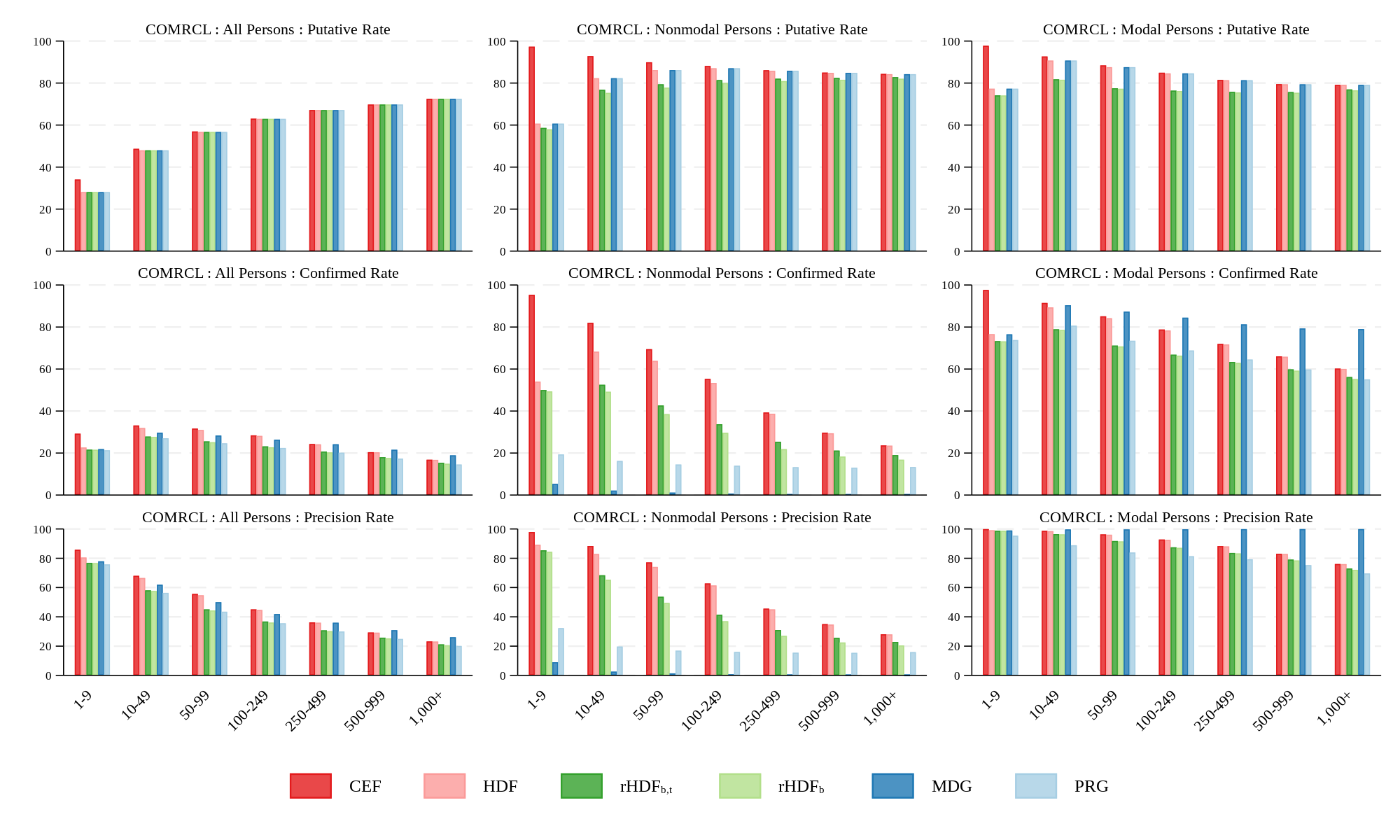
Notes: The denominator used in the first column is the COMCRL Population column in Table LABEL:tab:reid_blockpop, which totals to 286,700,000. The denominator in the second column is the COMRCL population in Table LABEL:tab:reid_blockpop_nm, and the denominator in the third column is the COMRCL population in Table LABEL:tab:reid_blockpop_m. The denominators in the second and third columns sum to 106,300,000 because only that subset of COMRCL records can be classified as modal and nonmodal from the CEF. See Table 3.
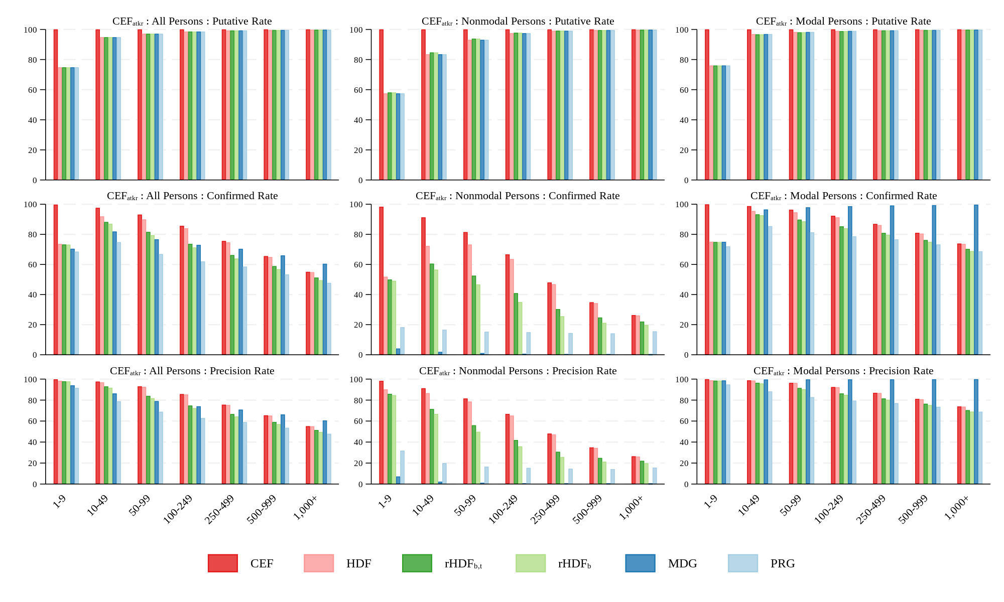
Notes: The denominator used in the first column is the Population column in Table LABEL:tab:reid_blockpop, which totals to 276,000,000. The denominator in the second column is the population in Table LABEL:tab:reid_blockpop_nm, and the denominator in the third column is the population in Table LABEL:tab:reid_blockpop_m. The denominators in the second and third columns sum to 276,000,000 because all records in can be classified as modal and nonmodal from the CEF. See Table 3.
For comparing and contrasting the nonmodal and modal persons results, the interpretation does not depend on the attacker database, so we characterize them generically. In these figures, nonmodal data-defined persons are the vulnerable population. Except for blocks with populations of 1-9 persons, CEF, HDF, , , MDG, and PRG putatively reidentify nonmodal persons at essentially the same rates because SF1 Tables P12 and 14 contain all the information used for putative reidentifications. It is the confirmation and precision rates that reveal the contrast with the modal person subpopulation. In blocks with 1-9 persons, the HDF, , and have essentially identical confirmation and precision rates, whereas the MDG baseline is nearly zero for both confirmation and precision rates, and the PRG baseline is greater than the MDG but substantially less than either or . As the population in the census block increases, the confirmation and precision rates of and decline but remain high, much closer to the rates for CEF and HDF than MDG (always essentially zero) and approaching proportional guessing only for the most populous census blocks. Even though there are 125 possible nonmodal {race, ethnicity} combinations, the reidentification precision rate of the reconstructed data is greater than 50% for 23,765,000 persons living in census blocks with populations of 1-99 persons (more than of all nonmodal data-defined persons) compared to essentially 0 for the modal guesser. For this same group, the smallest gain in the reidentification precision rate relative to the proportional guesser is 36.8 percentage points. This enormous gain in accuracy occurs only because the nonmodal person’s data were used in the SF1 tabulations. When the vulnerable population is defined as persons who differ from the predominant characteristics in small neighborhoods, in this case nonmodal {race, ethnicity} persons in lower-population census blocks, the statistical baselines either fail completely (MDG) or fair no better than chance (PRG), but the reconstructed microdata are correct at rates that approach the correctness of the confidential data themselves as the neighborhood population decreases.
Our interpretation of the mechanism causing the increased precision for vulnerable persons—the use of their specific response in the census tabulations—is further supported by examining the results for modal data-defined persons. In this case, the reidentification precision rates convey the main result. As expected, the modal guesser (MDG) has essentially perfect precision because our modal population was defined using the actual mode in the confidential data, and that is also the mode in the overwhelming majority of published block-level {race, ethnicity} tables, even in the census blocks with population of 1-9 persons, where the MDG precision rate takes its smallest value of 98.7%. But even in this nonvulnerable population, where the deck is deliberately stacked in favor of the modal guesser, and have reidentification precision rates substantially closer to the CEF and HDF than the proportional guesser. In blocks with populations of 1-9 persons, the precision rate of is at most 0.3 percentage points worse than HDF, while the precision rate of PRG is at best 4.0 percentage points worse than HDF. As the block population increases, the reidentification precision rates for CEF, HDF, , and all decrease, approaching but remaining greater than the precision rate for PRG. Even in the largest population census blocks, the precision of is at worst 3.3 percentage points lower than HDF while the precision of PRG is at best 4.8 percentage points lower than HDF. Even for less vulnerable populations, in this case modal {race, ethnicity} persons living in any size census block, the reconstructed microdata outperform proportional guessing, delivering prediction accuracy closer to the performance of the confidential data than this statistical baseline. Of course, the modal guesser outperforms even the confidential data in this case because of way it is defined.
8.3. Results for the Most Vulnerable Populations
We now discuss the results for the most tightly constrained definition of the vulnerable population—nonmodal data-defined persons living in blocks with 0 solution variability whose reconstructed records are population uniques for {block, sex, agebin}. Panel A of Table LABEL:tab:nm_solvar shows the results for nonmodal persons living in 0 solution variability blocks and Panel B shows the results for the subset of these persons who are population unique on {block, sex, agebin}. Recalling that population uniqueness on {block, sex, agebin} implies population uniquness on {block, sex, age} and that 0 solution variability implies that the record in the reconstructed data is provably the same as the record in HDF without referencing any confidential data, Table LABEL:tab:nm_solvar establishes that the reidentification precision rates of and HDF are essentially identical 91.2 versus 93.0 in COMCRL and 95.2 versus 95.6 in . These reidentification precisions are far in excess of the modal guesser’s (2.5 at best) or the proportional guesser’s (20.2). Thus, the correct {race, ethnicity} has been exposed for more than 19 of 20 persons in the population of nonmodal, 0-, {block, sex, agebin} uniques—essentially the same exposure as publishing the HDF itself, and only five percentage points worse than publishing the CEF itself. Statistical baselines are either almost always wrong or wrong for 4 of 5 persons in this vulnerable population. These results definitively show that the published SF1 tables result in confidentiality breaches since the high statistical precision of the reconstructed microdata is only possible because the target person’s data were used in the SF1 tabulations. If HDF was unsafe to release under the 2010 Census disclosure limitation framework, then the Summary File 1 statistics in Table 2 were also unsafe to release.
| Attacker ( in Alg. 3): COMRCL | Attacker ( in Alg. 3): | |||||||
|---|---|---|---|---|---|---|---|---|
| Popu- | Puta- | Con- | Preci- | Popu- | Puta- | Con- | Preci- | |
| Data ( in | lation | tive | firmed | sion | lation | tive | firmed | sion |
| Algorithm 3) | () | () | () | (%) | () | () | () | (%) |
| Panel A: Nonmodal Persons | ||||||||
| CEF | 2,098 | 1,925 | 1,633 | 84.8 | 6,517 | 6,517 | 5,727 | 87.9 |
| HDF | 2,098 | 1,646 | 1,278 | 77.7 | 6,517 | 5,189 | 4,209 | 81.1 |
| 2,098 | 1,557 | 1,009 | 64.8 | 6,517 | 5,305 | 3,634 | 68.5 | |
| 2,098 | 1,516 | 914 | 60.3 | 6,517 | 5,304 | 3,369 | 63.5 | |
| MDG | 2,098 | 1,646 | 33 | 2.0 | 6,517 | 5,189 | 88 | 1.7 |
| PRG | 2,098 | 1,646 | 274 | 16.6 | 6,517 | 5,189 | 890 | 17.2 |
| MDF | 2,098 | 593 | 103 | 17.3 | 6,517 | 1,866 | 353 | 18.9 |
| 2,098 | 593 | 103 | 17.3 | 6,517 | 1,866 | 352 | 18.9 | |
| 2,098 | 1,733 | 1,236 | 71.3 | 6,517 | 6,242 | 4,693 | 75.2 | |
| 2,098 | 1,255 | 680 | 54.1 | 6,517 | 4,270 | 2,482 | 58.1 | |
| Panel B: Nonmodal Uniques on | ||||||||
| CEF | 908 | 834 | 834 | 100.0 | 3,364 | 3,364 | 3,364 | 100.0 |
| HDF | 908 | 649 | 625 | 96.4 | 3,364 | 2,418 | 2,311 | 95.6 |
| 908 | 587 | 560 | 95.4 | 3,364 | 2,418 | 2,301 | 95.2 | |
| 908 | 565 | 537 | 95.0 | 3,364 | 2,418 | 2,237 | 92.5 | |
| MDG | 908 | 649 | 21 | 3.3 | 3,364 | 2,418 | 61 | 2.5 |
| PRG | 908 | 649 | 136 | 20.9 | 3,364 | 2,418 | 488 | 20.2 |
| MDF | 908 | 193 | 42 | 21.6 | 3,364 | 671 | 147 | 21.8 |
| 908 | 193 | 42 | 21.7 | 3,364 | 671 | 147 | 21.8 | |
| 908 | 723 | 710 | 98.2 | 3,364 | 3,194 | 3,111 | 97.4 | |
| 908 | 485 | 371 | 76.4 | 3,364 | 2,014 | 1,568 | 77.9 | |
| Notes: Counts rounded to four significant digits to conform to disclosure limitation | ||||||||
| requirements. The rows labeled and MDF (light gray highlight) are the analogues | ||||||||
| of and HDF, respectively, when the 2020 Census DAS is applied to the 2010 CEF. | ||||||||
| The rows labeled and (medium gray highlight) are the analogues | ||||||||
| of when alternative swapping parameters are used. See Section 10. Population for | ||||||||
| attacker COMRCL is data-defined nonmodal person records in COMRCL that match CEF | ||||||||
| on the feature set {pik, block}. Population for attacker is all data-defined | ||||||||
| nonmodal persons in CEF. | ||||||||
9. The 2010 Census Statistical Disclosure Limitation Framework Did Not Meet the Census Bureau’s Own Standards
The results of our experiment show that it is possible to create an extremely accurate reconstruction (95% binned-age agreement, see Table LABEL:tab:reconstruction_by_blocksize) of the underlying HDF microdata from publicly available sources, effectively undoing any confidentiality protection resulting from releasing tabular summaries instead of releasing the same features as a microdata extract of the universe of HDF person records. There was no reconstruction solution variability for of populated blocks, meaning that the reconstructed records in were the exact image of the records in HDF for the feature set {block, sex, agebin, race, ethnicity}. For these blocks, housing-unit swapping and synthetic data for the group quarters population are the only sources of uncertainty about their correctness relative to the CEF. These SDL measures do affect the accuracy of the reconstruction relative to the CEF, especially in the blocks with the smallest population sizes (74% agreement in blocks with population size of 0-9), but the accuracy is still very high overall (and could be higher for attackers who attempt to undo the swapping). When the reconstructed data are linked to an external dataset, an attacker can learn extra characteristics about members of their dataset that they previously did not know, and could not learn statistically, with very high accuracy for select publicly identifiable subgroups. The attacker’s successful inference depends on several factors. First, the more accurately the external dataset matches the linking variables {block, sex, agebin}, the more records the attacker will successfully link and the better the inference about the value of the other census responses will be. In our experiment, only about of the records in our low quality commercial data were correct matches to the CEF on these linking variables. Consequently, even though we could make a large number of putative matches, many were not confirmed–not because of incorrect inference on the unknown characteristics {race, ethnicity}, but because the characteristics on the external dataset were inaccurate quasi-identifiers. In our experiments using a much more accurate external database (either the or the subset of records in the commercial database that matched the CEF) the confirmation and precision rates were much higher. As the accuracy of the external data improves, the success of our attack improves, indicating that any conclusions based on the relatively low quality of commercial name and address databases in 2010 should be tempered by the improved quality of such data by 2020.
Our reconstruction-abetted reidentification atack was much more accurate in successfully inferring the of records with a value that was different than the most common (modal) in the block in comparison with the baseline inferential methods of guessing the modal {race, ethnicity} and guessing the {race, ethnicity} with probability proportional to publicly released counts. It also vastly outperformed the baseline methods when making inferences about records that were unique and had nonmodal , facts that the attacker could infer exactly in blocks with zero solution variability without consulting any confidential data. Therefore, while it is possible to make accurate inferences with these baseline methods when statistical information is used, the reconstruction-abetted reidentification attack exposes the vulnerability of the confidentiality protections by permitting accurate inferences on persons with statistically uncommon and rare characteristics. The accurate inference of the race and ethnicity of a person who is a population unique is only possible because that person’s record was available in . Such an inference is nonstatistical using the framework laid out in Section 5. Record-level data swapping marginally reduced the number of records in the at risk for a putative match, but it had no discernible effect on the precision of nonstatistical inferences for the vast majority of records.
The conclusion from this analysis is that the disclosure avoidance system applied to the 2010 Census did not meet the requirements for approval set forth by the Census Bureau’s Data Stewardship Executive Policy (DSEP) Committee for 2010 Census publications and, in light of current algorithmic and computational capabilities, it is not viable for future use. The results of the this experiment motivated the Census Bureau to change the SDL methods used for the 2020 Census [abowd2018us]. Instead of record swapping, synthetic group quarters data, and aggregation, the Bureau used differentially private mechanisms for all tabulations from the 2020 Census [Abowd20222020]. Had the Census Bureau continued to use the 2010 technology for 2020, it would have had to use the same rules for microdata as for tabular data, likely resulting in a much higher swap rate and a large amount of suppression of block-level data.
10. The 2020 Census Statistical Disclosure Limitation System Addressed the Failures of the 2010 System
Our final discussion addresses whether any SDL method can simultaneously defend against reidentification attacks and other nonstatistical uses while allowing publication of data that are fit for use in the primary applications. [christ:radway:bellovin:2020] demonstrated that the Census Bureau’s differentially private disclosure avoidance system could provide fitness-for-use in the redistricting application comparable to swapping but with superior confidentiality protection. They also noted that “[s]wapping places a disproportionate privacy burden on minority groups,” while differential privacy protections apply to all sub-populations. These results, which we confirm in this paper, are in contrast to the erroneous conclusions drawn by [kenny:et:al:2021] who calculated percentage changes incorrectly for small populations and failed to distinguish between generalizable and privacy-violating inferences [jarmin:etal:2023]. [wright:irimata:2021] demonstrated that the 2020 Census Redistricting Data (P.L. 94-171) Summary File was fit for use in redistricting and scrutiny under Section 2 of the 1965 Voting Rights Act.
On October 20, 2022, DSEP approved the final production settings for the 2020 Census disclosure avoidance system as applied to the Demographic and Housing Characteristics (DHC) File, the successor to the 2010 Summary File 1 used in this paper. DHC was produced using an extension of the algorithms described in [Abowd20222020] that includes the 2020 Census version of the tables used in this paper [cumings-menon:etal:2023]. The statistical summaries presented for the DSEP decision included an analysis of the effectiveness of the same reconstruction-abetted reidentification attack studied here based on the 2010 Census. The analysis compared the confidentiality protections from the original SF1 tables shown in Tables 2, 3 and 4 with the protection afforded by the differentially private disclosure avoidance system, when executed at the DHC production settings applied to the 2010 Census data, and the protection afforded by housing unit-level data swapping at rates of 5% and , i.e., swapping 5% or half of all housing units to a new location in a different block, tract, or elsewhere in the state. See Appendix C for details.
Table LABEL:tab:agree_blockpop_mdf shows the agreement rates overall and by census block size between the 2010 CEF and
-
•
HDF,
-
•
,
-
•
,
-
•
—reconstructed Microdata Detail File (MDF), [Abowd20222020], the production version output of the differentially private DAS for the DHC when applied to 2010 Census data and processed into the equivalents of the Table 2 statistics,
-
•
MDF—actual MDF from the same 2020 DAS output; i.e., not processed into tables, so there is no reconstruction of the microdata—these are the actual microdata from which DHC was tabulated,
-
•
—the results of the 5% swap-rate experiment when similarly processed.
-
•
—the results of the 50% swap-rate experiment when process through our reconstruction-abetted reidentification attack,
The , MDF, and reduce the agreement with the 2010 CEF substantially, with the and MDF reducing agreement more than . The agrees with the CEF at essentially the same rate as except for blocks with populations of 1-9 persons, where HDF, , and all agree with the CEF for 74.0% of records using binned age while agrees with 94.9% of these records. The experimental swap methodology did not single-out low population blocks for relatively greater swapping.
| Census | ||||||
|---|---|---|---|---|---|---|
| Data ( in | Block | Population | Agreement () | Agreement (%) | ||
| Algorithm 2) | Size | () | Exact Age | Binned Age | Exact Age | Binned Age |
| HDF-CEF | All | 308,746 | 297,200 | 297,600 | 96.3 | 96.4 |
| -CEF | All | 308,746 | 143,800 | 283,600 | 46.6 | 91.9 |
| -CEF | All | 308,746 | 132,200 | 276,900 | 42.8 | 89.7 |
| -CEF | All | 308,746 | 58,520 | 113,100 | 18.9 | 36.6 |
| MDF-CEF | All | 308,746 | 75,950 | 113,300 | 24.6 | 36.7 |
| -CEF | All | 308,746 | 144,500 | 281,200 | 46.8 | 91.1 |
| -CEF | All | 308,746 | 100,800 | 193,200 | 32.7 | 62.6 |
| HDF-CEF | 1-9 | 8,070 | 5,866 | 5,973 | 72.7 | 74.0 |
| -CEF | 1-9 | 8,070 | 2,419 | 5,971 | 30.0 | 74.0 |
| -CEF | 1-9 | 8,070 | 2,325 | 5,968 | 28.8 | 74.0 |
| -CEF | 1-9 | 8,070 | 232 | 647 | 2.9 | 8.0 |
| MDF-CEF | 1-9 | 8,070 | 276 | 647 | 3.4 | 8.0 |
| -CEF | 1-9 | 8,070 | 3,278 | 7,660 | 40.6 | 94.9 |
| -CEF | 1-9 | 8,070 | 1,803 | 4,280 | 22.3 | 53.0 |
| HDF-CEF | 10-49 | 67,598 | 63,460 | 63,580 | 93.9 | 94.1 |
| -CEF | 10-49 | 67,598 | 29,500 | 62,870 | 43.6 | 93.0 |
| -CEF | 10-49 | 67,598 | 28,990 | 62,330 | 42.9 | 92.2 |
| -CEF | 10-49 | 67,598 | 4,999 | 12,330 | 7.4 | 18.2 |
| MDF-CEF | 10-49 | 67,598 | 6,216 | 12,320 | 9.2 | 18.2 |
| -CEF | 10-49 | 67,598 | 30,320 | 63,370 | 44.9 | 93.8 |
| -CEF | 10-49 | 67,598 | 18,110 | 38,330 | 26.8 | 56.7 |
| HDF-CEF | 50-99 | 69,073 | 66,560 | 66,630 | 96.4 | 96.5 |
| -CEF | 50-99 | 69,073 | 31,280 | 64,330 | 45.3 | 93.1 |
| -CEF | 50-99 | 69,073 | 30,600 | 63,130 | 44.3 | 91.4 |
| -CEF | 50-99 | 69,073 | 8,350 | 18,830 | 12.1 | 27.3 |
| MDF-CEF | 50-99 | 69,073 | 10,670 | 18,820 | 15.5 | 27.2 |
| -CEF | 50-99 | 69,073 | 31,190 | 63,300 | 45.2 | 91.6 |
| -CEF | 50-99 | 69,073 | 20,200 | 41,180 | 29.2 | 59.6 |
| HDF-CEF | 100-249 | 80,021 | 78,370 | 78,420 | 97.9 | 98.0 |
| -CEF | 100-249 | 80,021 | 34,690 | 71,940 | 43.4 | 89.9 |
| -CEF | 100-249 | 80,021 | 36,840 | 73,810 | 46.0 | 92.2 |
| -CEF | 100-249 | 80,021 | 15,030 | 30,810 | 18.8 | 38.5 |
| MDF-CEF | 100-249 | 80,021 | 19,750 | 30,790 | 24.7 | 38.5 |
| -CEF | 100-249 | 80,021 | 36,310 | 71,880 | 45.4 | 89.8 |
| -CEF | 100-249 | 80,021 | 25,740 | 50,530 | 32.2 | 63.2 |
| HDF-CEF | 250-499 | 42,911 | 42,320 | 42,340 | 98.6 | 98.7 |
| -CEF | 250-499 | 42,911 | 18,170 | 37,960 | 42.3 | 88.5 |
| -CEF | 250-499 | 42,911 | 20,750 | 39,240 | 48.3 | 91.4 |
| -CEF | 250-499 | 42,911 | 12,220 | 22,570 | 28.5 | 52.6 |
| MDF-CEF | 250-499 | 42,911 | 16,290 | 22,600 | 38.0 | 52.7 |
| -CEF | 250-499 | 42,911 | 20,470 | 38,250 | 47.7 | 89.2 |
| -CEF | 250-499 | 42,911 | 15,830 | 29,030 | 36.9 | 67.7 |
| HDF-CEF | 500-999 | 27,029 | 26,720 | 26,740 | 98.9 | 98.9 |
| -CEF | 500-999 | 27,029 | 14,220 | 24,550 | 52.6 | 90.8 |
| -CEF | 500-999 | 27,029 | 11,380 | 23,480 | 42.1 | 86.9 |
| -CEF | 500-999 | 27,029 | 10,280 | 17,210 | 38.0 | 63.7 |
| MDF-CEF | 500-999 | 27,029 | 13,540 | 17,310 | 50.1 | 64.0 |
| -CEF | 500-999 | 27,029 | 14,090 | 24,060 | 52.1 | 89.0 |
| -CEF | 500-999 | 27,029 | 11,480 | 19,130 | 42.5 | 70.8 |
| HDF-CEF | 1,000+ | 14,043 | 13,930 | 13,940 | 99.2 | 99.3 |
| -CEF | 1,000+ | 14,043 | 8,835 | 12,870 | 62.9 | 91.7 |
| -CEF | 1,000+ | 14,043 | 6,009 | 12,120 | 42.8 | 86.3 |
| -CEF | 1,000+ | 14,043 | 7,407 | 10,670 | 52.8 | 76.0 |
| MDF-CEF | 1,000+ | 14,043 | 9,204 | 10,820 | 65.5 | 77.0 |
| -CEF | 1,000+ | 14,043 | 8,798 | 12,720 | 62.7 | 90.6 |
| -CEF | 1,000+ | 14,043 | 7,678 | 10,730 | 54.7 | 76.4 |
| Notes: Census Block Size is the population range in the census block. Counts rounded to | ||||||
| four significant digits, except block populations, to conform to disclosure limitation | ||||||
| requirements. Agreement percentages use the block populations in that row as the base. | ||||||
| The rows labeled and MDF (light gray highlight) are the analogues of | ||||||
| and HDF, resp., when the 2020 Census DAS is applied to the 2010 CEF. Rows labeled | ||||||
| and (medium gray highlight) are the results of applying the full | ||||||
| reconstruction-abetted reidentification attack to the specially swapped versions of HDF | ||||||
| described in the main text. | ||||||
Figures 5 and 6 compare the putative reidentification, confirmed reidentification, and reidentification precision rates by census block size when the attacker is COMCRL or , respectively. Their interpretation is identical to the interpretation of Figures 3 and 4. Detailed statistics can be found in Appendix Tables LABEL:tab:reid_blockpop_mdf, LABEL:tab:reid_blockpop_nm_mdf, and LABEL:tab:reid_blockpop_m_mdf.
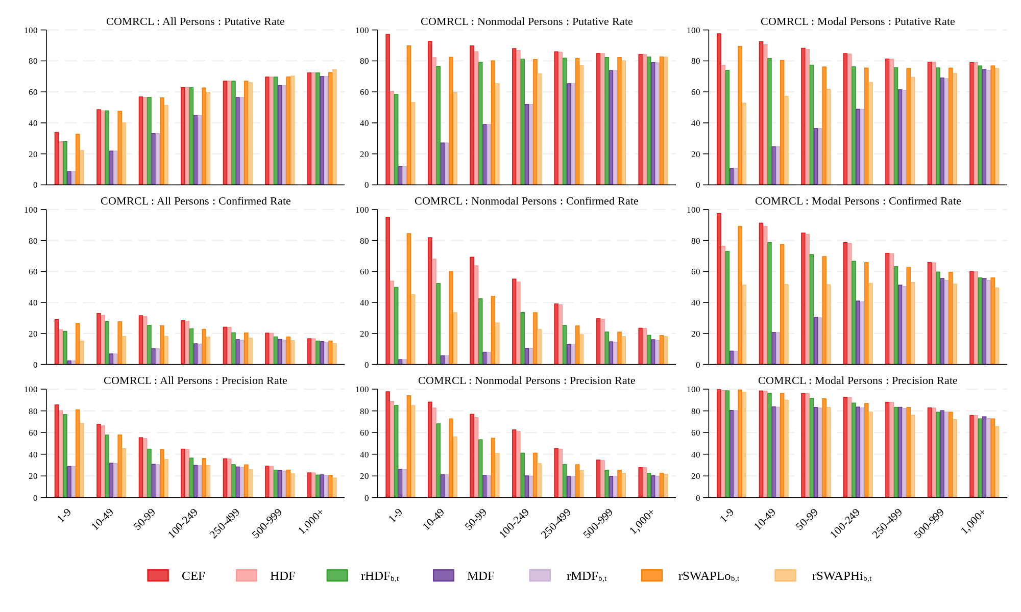
Notes: The denominator used in the first column is the COMCRL Population column in Table LABEL:tab:reid_blockpop_mdf, which totals to 286,700,000. The denominator in the second column is the COMRCL population in Table LABEL:tab:reid_blockpop_nm_mdf, and the denominator in the third column is the COMRCL population in Table LABEL:tab:reid_blockpop_m_mdf. The denominators in the second and third columns sum to 106,300,000 because only that subset of COMRCL records can be classified as modal and nonmodal from the CEF. See Table 3.
Only the output of the 2020 DAS ( and MDF) and succeed in reducing putative reidentification rates because only those SDL treatments introduce substantial noise in the quasi-identifiers {block, sex, agebin}. Without noise in those quasi-identifiers, putative reidentification rates will always be very close to those of the CEF.
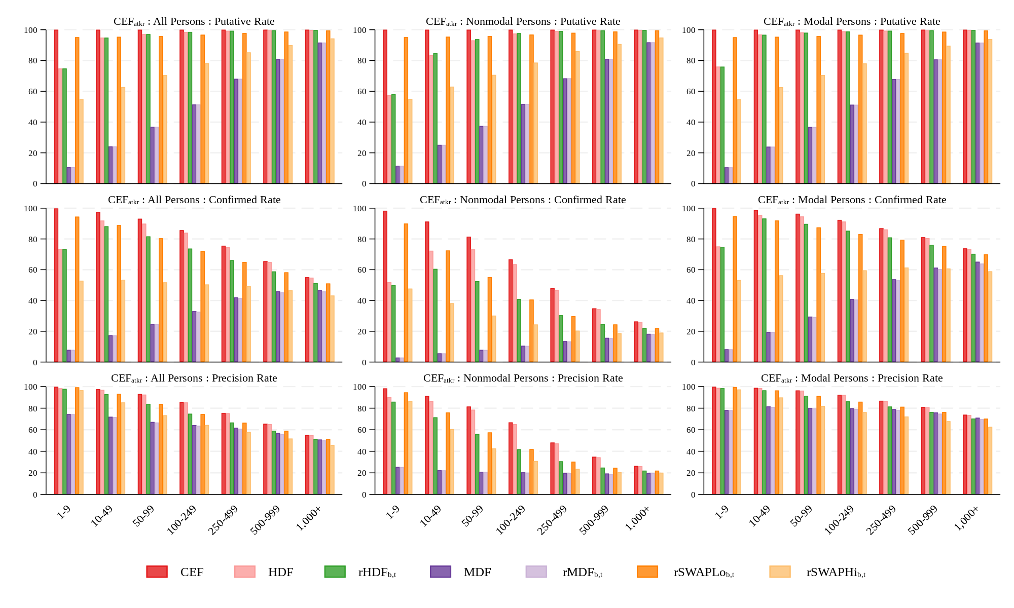
Notes: The denominator used in the first column is the Population column in Table LABEL:tab:reid_blockpop_mdf, which totals to 276,000,000. The denominator in the second column is the population in Table LABEL:tab:reid_blockpop_nm_mdf, and the denominator in the third column is the population in Table LABEL:tab:reid_blockpop_m_mdf. The denominators in the second and third columns sum to 276,000,000 because all records in can be classified as modal and nonmodal from the CEF. See Table 3.
The second important feature of Figures 5 and 6 is the very low, nearly uniform by block size, reidentification precision rates for and MDF for the nonmodal data-defined persons (middle column). These are the only SDL treatments shown in the figures that accomplish this reduction. As the data in Appendix Table LABEL:tab:reid_blockpop_nm_mdf show, the reidentification precision rate for nonmodal persons never exceeds 26.4% and averages 20.1% to 20.4%. An attacker using the methods in this paper would be wrong four times in five guessing the {race, ethnicity} from either the reconstructed MDF, , or the MDF itself. This is essentially the same as the failure rate on nonmodal persons for the PRG statistical baseline, 16.0% to 16.7%, shown in Appendix Table LABEL:tab:reid_blockpop_nm.
Table LABEL:tab:nm_solvar contains the final piece of evidence that the 2020 DAS effectively countered reconstruction-abetted reidentification attacks as we have modeled them here. For the nonmodal persons living in 0 solution variability blocks who are population unique on {block, sex, agebin} (Panel B), the reidentification precision rates of and MDF vary between 19.7% and 21.8%, essentially identical to the precision rates for nonmodal persons in general. Neither the low nor high swap rate experiments deliver precision rates for this vulnerable population below 72.2%. An attacker using and our methods would be correct about the population unique nonmodal {race, ethnicity} approximately three times out of four, even though 50% of the housing unit records have been swapped.
The replication archive also contains an ExcelTM (rmdf_bt_0solva_extract.xlsx) workbook with reconstructed MDF records from the same 29 census tracts in which every block has 0 solution variability for that are shown in rhdf_bt_0solvar_extract.xlsx. Tags also identify every row that is population unique on {block, sex, agebin} and {block, sex, agebin, race, ethnicity} in the spreadsheet. Inspection of the record-level data in these two workbooks shows how the DAS reduced both putative reidentification and reidentification precision rates.
Because we have demonstrated that the tabular and microdata formats for publishing data processed by the 2020 DAS are properly protected either when reconstructed from DHC tables into or as the MDF itself, both could be safely released. The 2020 DAS, therefore, demonstrably fixes the inconsistency flaw in the 2010 Census SDL framework.
We have only considered the ability of the 2020 DAS to defend against reconstruction-abetted reidentification attacks; however, both the redistricting and DHC data products were extensively tuned for accuracy. These results are available in other sources [USCB:2023:DHC:DEMO:Metrics, Abowd20222020, cumings-menon:etal:2023] and in the replication archive for this paper. The replication archive also contains the same extensive set of metrics for and . The low swap rate experiment has accuracy comparable to SF1. The high swap rate experiment has accuracy far worse than the production DHC on most statistics.
The other feasible alternative to the 2020 DAS was a variant of the suppression methods used in the 1980 Census. Suppression can defend against an important subset of reconstruction attacks—isolating the records of population uniques; however, successful suppression systems, such as the one used for economic censuses [cox:1995], require both primary and complementary suppression. Appendix D lays out the rules used for the 1980 Census as we adapted them to testing suppression for the 2020 Census. Only primary and whole table suppression were used. Without complementary suppression there is no provable defense against reconstruction of population unique records. We considered only the four primary tables in the P.L. 94-171 Redistricting Data Summary File (P8–P11 in Summary File 1). Appendix Tables 18 and 19 show that the use of just the 1980 Census primary suppression rules would have resulted in zeroing out up to 83.8% of the cells in these tables, suppressing up to 87.7% of the block-level redistricting tables, and suppressing 38.7% of the other block-level tables in the 2010 SF1. Suppression destroys the redistricting use case—missing block-level tables prevent the creation of new voting districts, which have unknown boundaries at the time of data publication. The new districts must have approximately equal populations and be drawn in compliance with Section 2 of the 1965 Voting Rights Act. This limitation of suppression was known in 1980 and constituted one of the main reasons for using swapping in the 1990 Census data [mckenna2018disclosure].
11. Conclusions
This paper directly addresses the concept at the heart of traditional statistical disclosure limitation: the claim that as long as there is some uncertainty regarding whether or not a particular respondent’s data were used in a particular statistic the agency has provided “plausible deniability.” We establish that the 2010 Census attacker does not need access to the confidential data to know (1) that the record is an exact copy of the confidential HDF (using the 38-age-bin schema) and (2) that the record is a population unique on the quasi-identifiers {block, sex, agebin} used for a classic record-linkage attack. While this is strictly true for “only” 97 million persons, adding more tables and more features can only increase this number. If the reconstructed microdata meet the conditions for a microdata-based record-linkage attack, then such an attack must be defended in the SDL framework. Therefore, the plausible deniability argument turns on whether the 2010 Census aggregation and swapping were adequate. We argued here that they were not. In particular, if the released tabular data have reidentification precision rates that are essentially identical to the original confidential data, then either those data could have been released without aggregation, which the Census Bureau has consistently argued would violate Title 13, or the tabular data are too disclosive, which is what we conclude. The burden of proof now lies with traditional SDL to defend the status quo or accept the consequences of our research.
This paper has also demonstrated that the decision to replace the SDL system used for the 2010 Census was based on sound scientific evidence that those methods would fail if applied to the 2020 Census and/or would lead to unacceptable data accuracy loss. First, we demonstrated that based on only 5 billion of the 150 billion statistics published from the 2010 Census, the confidential microdata from the tabulation input file, the Hundred-percent Detail File, could be recreated with at least 95% accuracy on the schema used for all block-level data. This image of the 2010 HDF, , fails three contemporaneous confidentiality requirements for the 2010 Census: (i) it is not a sample; (ii) the minimum population in the geographic identifier is 1 person, not 100,000; (iii) the minimum national population for cells in one-dimensional marginals is less than 10,000. Similar criteria are still in place for public-use microdata samples for other Census Bureau household surveys. Second, we demonstrated that the Census Bureau was correct to insist on minimum populations in microdata for both the geographic identifiers and demographic characteristics because for more than 70% of all blocks, the records in are provably identical to their counterparts in the HDF using the binned-age schema; hence, there is no confidentiality protection from aggregation over the geographic identifier population. Third, we demonstrated that could be used to make high-precision confidentiality-violating inferences: (i) the reidentification precision rate on inferences for nonmodal vulnerable populations is at least 62% and at worst 95% whereas the best precision rate for scientific inferences in vulnerable populations is 32%, and a modal guesser never exceeds 9% precision. Finally, we demonstrated that the differentially private SDL methods applied to the 2020 DHC, the successor to the 2010 SF1, successfully counter this reconstruction-abetted reidentification attack by greatly reducing the putative reidentification rates and by limiting the precision rates on nonmodal vulnerable populations to at most 26.4%. Although such a demonstration does not mean the public 2020 Census data are protected against an arbitrary attack into the indefinite future, it does mean that they are substantially better protected than they would have been had the methods applied to the 2010 Census been used.
Disclosure Statement
The research presented in this article was initiated, funded and supervised by the U.S. Census Bureau. All authors were either employees or contractors of the Census Bureau while performing their contributions.
Disclaimer and Acknowledgments
The views and opinions expressed in this paper are those of the authors and not the U.S. Census Bureau. Research was conducted under Project ID: P-7502798. John Abowd, Simson Garfinkel, Ramy Tadros, and Lars Vilhuber worked in their personal capacities and without access to any confidential data after leaving the Census Bureau (Abowd, Garfinkel, and Vilhuber) and Galois (Tadros), respectively, to assist in preparing the manuscript for publication. Statistics reported were released under DRB Clearance numbers CBDRB-FY20-DSEP-001, CBDRB-FY22-DSEP-003, CBDRB-FY22-DSEP-004, and CBDRB-FY23-0152.
Data availability
The public replication archive is located at https://github.com/uscensusbureau/recon_replication. The archive contains all tables and figures in this paper in an ExcelTM workbook. The archive also contains pointers to the official versions of all public data used in this paper, the complete code base, and a description of the workflow that meets current scientific best practices as defined by the American Economic Association https://aeadataeditor.github.io/. Census Bureau Data Stewardship Policy DS-027 https://www2.census.gov/foia/ds_policies/ds027.pdf permitted the editor and referees of journals that reviewed this work to independently verify the correctness of the calculations done on the confidential 2010 Census and commercial data used in this paper.
Contributions
-
•
Conceptualization: JMA, TA, SLG, DK, PL, LV
-
•
Data curation: NG, RAR, LV
-
•
Formal Analysis: TA, SLG, DK, PL
-
•
Methodology: JMA, TA, RA, DD, SD, SLG, NG, DK, PL, EL, SM, RAR, RNT, LV
-
•
Investigation: DD, SD, SLG, NG, DK, PL, EL, SM, RAR, RNT, LV
-
•
Software: TA, DD, SD, SLG, NG, PL, EL, SM, RAR, RNT, LV
-
•
Supervision: JMA
-
•
Writing – original draft: JMA, RA, SLG, NG, DK, PL, RAR, LV
-
•
Writing – review & editing: JMA, TA, RA, DD, SD, SLG, NG, DK, PL, EL, SM, RAR, RNT, LV
Appendix A Detailed Tables Referenced in Section 8
| Attacker ( in Alg. 3): COMRCL | Attacker ( in Alg. 3): | ||||||||
|---|---|---|---|---|---|---|---|---|---|
| Data | Census | Popu- | Puta- | Con- | Preci- | Popu- | Puta- | Con- | Preci- |
| ( in | Block | lation | tive | firmed | sion | lation | tive | firmed | sion |
| Alg. 3) | Size | () | () | () | (%) | () | () | () | (%) |
| CEF | All | 286,700 | 167,500 | 82,760 | 49.4 | 276,000 | 276,000 | 237,500 | 86.1 |
| HDF | All | 286,700 | 166,100 | 80,540 | 48.5 | 276,000 | 267,800 | 228,400 | 85.3 |
| All | 286,700 | 166,100 | 68,480 | 41.2 | 276,000 | 267,800 | 208,500 | 77.9 | |
| All | 286,700 | 166,100 | 67,450 | 40.6 | 276,000 | 267,800 | 203,100 | 75.9 | |
| MDG | All | 286,700 | 166,100 | 76,270 | 45.9 | 276,000 | 267,800 | 205,100 | 76.6 |
| PRG | All | 286,700 | 166,100 | 66,260 | 39.9 | 276,000 | 267,800 | 177,700 | 66.3 |
| CEF | 1-9 | 10,180 | 3,470 | 2,976 | 85.8 | 7,373 | 7,373 | 7,357 | 99.8 |
| HDF | 1-9 | 10,180 | 2,862 | 2,303 | 80.5 | 7,373 | 5,517 | 5,427 | 98.4 |
| 1-9 | 10,180 | 2,862 | 2,201 | 76.9 | 7,373 | 5,517 | 5,402 | 97.9 | |
| 1-9 | 10,180 | 2,862 | 2,196 | 76.7 | 7,373 | 5,517 | 5,395 | 97.8 | |
| MDG | 1-9 | 10,180 | 2,862 | 2,228 | 77.9 | 7,373 | 5,517 | 5,193 | 94.1 |
| PRG | 1-9 | 10,180 | 2,862 | 2,170 | 75.8 | 7,373 | 5,517 | 5,054 | 91.6 |
| CEF | 10-49 | 70,300 | 34,250 | 23,300 | 68.0 | 61,820 | 61,820 | 60,350 | 97.6 |
| HDF | 10-49 | 70,300 | 33,730 | 22,430 | 66.5 | 61,820 | 58,630 | 56,840 | 96.9 |
| 10-49 | 70,300 | 33,730 | 19,600 | 58.1 | 61,820 | 58,630 | 54,540 | 93.0 | |
| 10-49 | 70,300 | 33,730 | 19,430 | 57.6 | 61,820 | 58,630 | 53,840 | 91.8 | |
| MDG | 10-49 | 70,300 | 33,730 | 20,870 | 61.9 | 61,820 | 58,630 | 50,620 | 86.3 |
| PRG | 10-49 | 70,300 | 33,730 | 19,010 | 56.4 | 61,820 | 58,630 | 46,250 | 78.9 |
| CEF | 50-99 | 66,980 | 38,160 | 21,200 | 55.6 | 62,760 | 62,760 | 58,450 | 93.1 |
| HDF | 50-99 | 66,980 | 37,980 | 20,780 | 54.7 | 62,760 | 60,970 | 56,440 | 92.6 |
| 50-99 | 66,980 | 37,980 | 17,120 | 45.1 | 62,760 | 60,970 | 51,230 | 84.0 | |
| 50-99 | 66,980 | 37,980 | 16,860 | 44.4 | 62,760 | 60,970 | 49,880 | 81.8 | |
| MDG | 50-99 | 66,980 | 37,980 | 18,980 | 50.0 | 62,760 | 60,970 | 48,170 | 79.0 |
| PRG | 50-99 | 66,980 | 37,980 | 16,500 | 43.5 | 62,760 | 60,970 | 41,990 | 68.9 |
| CEF | 100-249 | 71,870 | 45,320 | 20,440 | 45.1 | 71,410 | 71,410 | 61,190 | 85.7 |
| HDF | 100-249 | 71,870 | 45,250 | 20,240 | 44.7 | 71,410 | 70,400 | 60,030 | 85.3 |
| 100-249 | 71,870 | 45,250 | 16,660 | 36.8 | 71,410 | 70,400 | 52,650 | 74.8 | |
| 100-249 | 71,870 | 45,250 | 16,350 | 36.1 | 71,410 | 70,400 | 50,890 | 72.3 | |
| MDG | 100-249 | 71,870 | 45,250 | 18,940 | 41.9 | 71,410 | 70,400 | 52,190 | 74.1 |
| PRG | 100-249 | 71,870 | 45,250 | 16,120 | 35.6 | 71,410 | 70,400 | 44,310 | 62.9 |
| CEF | 250-499 | 36,740 | 24,680 | 8,923 | 36.2 | 37,660 | 37,660 | 28,480 | 75.6 |
| HDF | 250-499 | 36,740 | 24,670 | 8,878 | 36.0 | 37,660 | 37,400 | 28,140 | 75.3 |
| 250-499 | 36,740 | 24,670 | 7,608 | 30.8 | 37,660 | 37,400 | 24,940 | 66.7 | |
| 250-499 | 36,740 | 24,670 | 7,459 | 30.2 | 37,660 | 37,400 | 24,090 | 64.4 | |
| MDG | 250-499 | 36,740 | 24,670 | 8,886 | 36.0 | 37,660 | 37,400 | 26,520 | 70.9 |
| PRG | 250-499 | 36,740 | 24,670 | 7,409 | 30.0 | 37,660 | 37,400 | 22,050 | 59.0 |
| CEF | 500-999 | 21,620 | 15,090 | 4,416 | 29.3 | 23,270 | 23,270 | 15,250 | 65.5 |
| HDF | 500-999 | 21,620 | 15,090 | 4,398 | 29.2 | 23,270 | 23,180 | 15,110 | 65.2 |
| 500-999 | 21,620 | 15,090 | 3,898 | 25.8 | 23,270 | 23,180 | 13,700 | 59.1 | |
| 500-999 | 21,620 | 15,090 | 3,809 | 25.3 | 23,270 | 23,180 | 13,230 | 57.1 | |
| MDG | 500-999 | 21,620 | 15,090 | 4,664 | 30.9 | 23,270 | 23,180 | 15,370 | 66.3 |
| PRG | 500-999 | 21,620 | 15,090 | 3,748 | 24.9 | 23,270 | 23,180 | 12,430 | 53.6 |
| CEF | 1,000+ | 8,976 | 6,510 | 1,510 | 23.2 | 11,670 | 11,670 | 6,432 | 55.1 |
| HDF | 1,000+ | 8,976 | 6,510 | 1,505 | 23.1 | 11,670 | 11,650 | 6,403 | 55.0 |
| 1,000+ | 8,976 | 6,510 | 1,380 | 21.2 | 11,670 | 11,650 | 5,986 | 51.4 | |
| 1,000+ | 8,976 | 6,510 | 1,339 | 20.6 | 11,670 | 11,650 | 5,779 | 49.6 | |
| MDG | 1,000+ | 8,976 | 6,510 | 1,699 | 26.1 | 11,670 | 11,650 | 7,056 | 60.6 |
| PRG | 1,000+ | 8,976 | 6,510 | 1,305 | 20.1 | 11,670 | 11,650 | 5,576 | 47.9 |
| PRG | 1,000+ | 8,976 | 6,510 | 1,305 | 20.1 | 11,670 | 11,650 | 5,576 | 47.9 |
| Notes: Census Block Size is the population range in the census block. Counts rounded to four | |||||||||
| significant digits to conform to disclosure limitation requirements. Population for attacker COMRCL | |||||||||
| is the total number of data-defined records in COMRCL that are also in the CEF universe (see | |||||||||
| Table 3). Population for attacker is the total number of data-defined CEF records. | |||||||||
| Attacker ( in Alg. 3): COMRCL | Attacker ( in Alg. 3): | ||||||||
|---|---|---|---|---|---|---|---|---|---|
| Data | Census | Popu- | Puta- | Con- | Preci- | Popu- | Puta- | Con- | Preci- |
| ( in | Block | lation | tive | firmed | sion | lation | tive | firmed | sion |
| Alg. 3) | Size | () | () | () | (%) | () | () | () | (%) |
| CEF | All | 17,320 | 15,330 | 9,746 | 63.6 | 65,850 | 65,850 | 42,070 | 63.9 |
| HDF | All | 17,320 | 14,780 | 8,967 | 60.7 | 65,850 | 62,530 | 38,120 | 61.0 |
| All | 17,320 | 13,910 | 6,147 | 44.2 | 65,850 | 62,810 | 27,180 | 43.3 | |
| All | 17,320 | 13,680 | 5,514 | 40.3 | 65,850 | 62,810 | 23,990 | 38.2 | |
| MDG | All | 17,320 | 14,780 | 170 | 1.2 | 65,850 | 62,530 | 580 | 0.9 |
| PRG | All | 17,320 | 14,780 | 2,473 | 16.7 | 65,850 | 62,530 | 10,000 | 16.0 |
| CEF | 1-9 | 150 | 146 | 143 | 97.9 | 480 | 480 | 472 | 98.3 |
| HDF | 1-9 | 150 | 91 | 81 | 89.2 | 480 | 276 | 249 | 90.2 |
| 1-9 | 150 | 88 | 75 | 85.4 | 480 | 279 | 240 | 86.0 | |
| 1-9 | 150 | 87 | 74 | 84.4 | 480 | 279 | 236 | 84.7 | |
| MDG | 1-9 | 150 | 91 | 8 | 9.0 | 480 | 276 | 20 | 7.2 |
| PRG | 1-9 | 150 | 91 | 29 | 32.3 | 480 | 276 | 88 | 31.8 |
| CEF | 10-49 | 2,733 | 2,537 | 2,242 | 88.4 | 9,545 | 9,545 | 8,713 | 91.3 |
| HDF | 10-49 | 2,733 | 2,250 | 1,865 | 82.9 | 9,545 | 7,971 | 6,904 | 86.6 |
| 10-49 | 2,733 | 2,099 | 1,435 | 68.4 | 9,545 | 8,084 | 5,777 | 71.5 | |
| 10-49 | 2,733 | 2,058 | 1,344 | 65.3 | 9,545 | 8,082 | 5,397 | 66.8 | |
| MDG | 10-49 | 2,733 | 2,250 | 59 | 2.6 | 9,545 | 7,971 | 184 | 2.3 |
| PRG | 10-49 | 2,733 | 2,250 | 444 | 19.7 | 9,545 | 7,971 | 1,587 | 19.9 |
| CEF | 50-99 | 3,957 | 3,558 | 2,748 | 77.2 | 13,740 | 13,740 | 11,200 | 81.5 |
| HDF | 50-99 | 3,957 | 3,411 | 2,527 | 74.1 | 13,740 | 12,790 | 10,060 | 78.6 |
| 50-99 | 3,957 | 3,143 | 1,688 | 53.7 | 13,740 | 12,900 | 7,221 | 56.0 | |
| 50-99 | 3,957 | 3,080 | 1,525 | 49.5 | 13,740 | 12,900 | 6,422 | 49.8 | |
| MDG | 50-99 | 3,957 | 3,411 | 47 | 1.4 | 13,740 | 12,790 | 157 | 1.2 |
| PRG | 50-99 | 3,957 | 3,411 | 576 | 16.9 | 13,740 | 12,790 | 2,111 | 16.5 |
| CEF | 100-249 | 5,055 | 4,457 | 2,797 | 62.8 | 18,670 | 18,670 | 12,460 | 66.8 |
| HDF | 100-249 | 5,055 | 4,400 | 2,700 | 61.4 | 18,670 | 18,210 | 11,870 | 65.2 |
| 100-249 | 5,055 | 4,116 | 1,706 | 41.4 | 18,670 | 18,260 | 7,645 | 41.9 | |
| 100-249 | 5,055 | 4,045 | 1,496 | 37.0 | 18,670 | 18,260 | 6,553 | 35.9 | |
| MDG | 100-249 | 5,055 | 4,400 | 35 | 0.8 | 18,670 | 18,210 | 132 | 0.7 |
| PRG | 100-249 | 5,055 | 4,400 | 706 | 16.0 | 18,670 | 18,210 | 2,798 | 15.4 |
| CEF | 250-499 | 2,703 | 2,328 | 1,063 | 45.6 | 10,970 | 10,970 | 5,275 | 48.1 |
| HDF | 250-499 | 2,703 | 2,320 | 1,047 | 45.1 | 10,970 | 10,870 | 5,142 | 47.3 |
| 250-499 | 2,703 | 2,219 | 687 | 31.0 | 10,970 | 10,880 | 3,337 | 30.7 | |
| 250-499 | 2,703 | 2,188 | 591 | 27.0 | 10,970 | 10,880 | 2,807 | 25.8 | |
| MDG | 250-499 | 2,703 | 2,320 | 12 | 0.5 | 10,970 | 10,870 | 51 | 0.5 |
| PRG | 250-499 | 2,703 | 2,320 | 359 | 15.5 | 10,970 | 10,870 | 1,586 | 14.6 |
| CEF | 500-999 | 1,807 | 1,536 | 537 | 35.0 | 7,846 | 7,846 | 2,735 | 34.9 |
| HDF | 500-999 | 1,807 | 1,534 | 532 | 34.7 | 7,846 | 7,812 | 2,690 | 34.4 |
| 500-999 | 1,807 | 1,490 | 383 | 25.7 | 7,846 | 7,813 | 1,945 | 24.9 | |
| 500-999 | 1,807 | 1,474 | 331 | 22.5 | 7,846 | 7,813 | 1,664 | 21.3 | |
| MDG | 500-999 | 1,807 | 1,534 | 6 | 0.4 | 7,846 | 7,812 | 28 | 0.4 |
| PRG | 500-999 | 1,807 | 1,534 | 236 | 15.4 | 7,846 | 7,812 | 1,116 | 14.3 |
| CEF | 1,000+ | 914 | 771 | 216 | 28.1 | 4,602 | 4,602 | 1,213 | 26.4 |
| HDF | 1,000+ | 914 | 770 | 215 | 28.0 | 4,602 | 4,595 | 1,203 | 26.2 |
| 1,000+ | 914 | 757 | 174 | 22.9 | 4,602 | 4,595 | 1,017 | 22.1 | |
| 1,000+ | 914 | 750 | 154 | 20.5 | 4,602 | 4,595 | 911 | 19.8 | |
| MDG | 1,000+ | 914 | 770 | 2 | 0.2 | 4,602 | 4,595 | 8 | 0.2 |
| PRG | 1,000+ | 914 | 770 | 122 | 15.9 | 4,602 | 4,595 | 717 | 15.6 |
| Notes: Census Block Size is the population range in the census block. Counts rounded to four | |||||||||
| significant digits to conform to disclosure limitation requirements. COMRCL and use | |||||||||
| only data-defined records. Only the 106,300,000 records in COMCRL that match CEF on the | |||||||||
| feature set {, } (see Table 3) can be used to identify a nonmodal person. For each | |||||||||
| attacker, the column Population shows the number of at-risk records. | |||||||||
| Attacker ( in Alg. 3): COMRCL | Attacker ( in Alg. 3): | ||||||||
|---|---|---|---|---|---|---|---|---|---|
| Data | Census | Popu- | Puta- | Con- | Preci- | Popu- | Puta- | Con- | Preci- |
| ( in | Block | lation | tive | firmed | sion | lation | tive | firmed | sion |
| Alg. 3) | Size | () | () | () | (%) | () | () | () | (%) |
| CEF | All | 88,930 | 77,620 | 73,010 | 94.1 | 210,100 | 210,100 | 195,400 | 93.0 |
| HDF | All | 88,930 | 76,300 | 71,570 | 93.8 | 210,100 | 205,200 | 190,300 | 92.7 |
| All | 88,930 | 69,260 | 62,330 | 90.0 | 210,100 | 204,900 | 181,300 | 88.5 | |
| All | 88,930 | 69,070 | 61,940 | 89.7 | 210,100 | 204,900 | 179,100 | 87.4 | |
| MDG | All | 88,930 | 76,300 | 76,100 | 99.7 | 210,100 | 205,200 | 204,500 | 99.7 |
| PRG | All | 88,930 | 76,300 | 63,790 | 83.6 | 210,100 | 205,200 | 167,700 | 81.7 |
| CEF | 1-9 | 2,901 | 2,836 | 2,833 | 99.9 | 6,893 | 6,893 | 6,886 | 99.9 |
| HDF | 1-9 | 2,901 | 2,243 | 2,222 | 99.1 | 6,893 | 5,241 | 5,177 | 98.8 |
| 1-9 | 2,901 | 2,151 | 2,126 | 98.8 | 6,893 | 5,239 | 5,163 | 98.5 | |
| 1-9 | 2,901 | 2,149 | 2,123 | 98.8 | 6,893 | 5,239 | 5,159 | 98.5 | |
| MDG | 1-9 | 2,901 | 2,243 | 2,220 | 99.0 | 6,893 | 5,241 | 5,173 | 98.7 |
| PRG | 1-9 | 2,901 | 2,243 | 2,141 | 95.4 | 6,893 | 5,241 | 4,966 | 94.8 |
| CEF | 10-49 | 23,020 | 21,330 | 21,050 | 98.7 | 52,270 | 52,270 | 51,630 | 98.8 |
| HDF | 10-49 | 23,020 | 20,880 | 20,570 | 98.5 | 52,270 | 50,660 | 49,930 | 98.6 |
| 10-49 | 23,020 | 18,830 | 18,170 | 96.5 | 52,270 | 50,550 | 48,760 | 96.5 | |
| 10-49 | 23,020 | 18,780 | 18,090 | 96.3 | 52,270 | 50,550 | 48,450 | 95.8 | |
| MDG | 10-49 | 23,020 | 20,880 | 20,810 | 99.7 | 52,270 | 50,660 | 50,440 | 99.6 |
| PRG | 10-49 | 23,020 | 20,880 | 18,570 | 88.9 | 52,270 | 50,660 | 44,660 | 88.2 |
| CEF | 50-99 | 21,680 | 19,170 | 18,450 | 96.3 | 49,020 | 49,020 | 47,250 | 96.4 |
| HDF | 50-99 | 21,680 | 18,990 | 18,250 | 96.1 | 49,020 | 48,180 | 46,380 | 96.3 |
| 50-99 | 21,680 | 16,810 | 15,430 | 91.8 | 49,020 | 48,070 | 44,010 | 91.5 | |
| 50-99 | 21,680 | 16,760 | 15,340 | 91.5 | 49,020 | 48,080 | 43,460 | 90.4 | |
| MDG | 50-99 | 21,680 | 18,990 | 18,940 | 99.7 | 49,020 | 48,180 | 48,010 | 99.7 |
| PRG | 50-99 | 21,680 | 18,990 | 15,930 | 83.9 | 49,020 | 48,180 | 39,880 | 82.8 |
| CEF | 100-249 | 22,380 | 19,010 | 17,640 | 92.8 | 52,740 | 52,740 | 48,730 | 92.4 |
| HDF | 100-249 | 22,380 | 18,940 | 17,540 | 92.6 | 52,740 | 52,200 | 48,150 | 92.3 |
| 100-249 | 22,380 | 17,100 | 14,960 | 87.5 | 52,740 | 52,140 | 45,000 | 86.3 | |
| 100-249 | 22,380 | 17,060 | 14,860 | 87.1 | 52,740 | 52,150 | 44,330 | 85.0 | |
| MDG | 100-249 | 22,380 | 18,940 | 18,900 | 99.8 | 52,740 | 52,200 | 52,060 | 99.7 |
| PRG | 100-249 | 22,380 | 18,940 | 15,410 | 81.4 | 52,740 | 52,200 | 41,510 | 79.5 |
| CEF | 250-499 | 10,920 | 8,901 | 7,860 | 88.3 | 26,690 | 26,690 | 23,200 | 86.9 |
| HDF | 250-499 | 10,920 | 8,885 | 7,831 | 88.1 | 26,690 | 26,520 | 23,000 | 86.7 |
| 250-499 | 10,920 | 8,278 | 6,921 | 83.6 | 26,690 | 26,510 | 21,610 | 81.5 | |
| 250-499 | 10,920 | 8,250 | 6,868 | 83.3 | 26,690 | 26,510 | 21,280 | 80.3 | |
| MDG | 250-499 | 10,920 | 8,885 | 8,874 | 99.9 | 26,690 | 26,520 | 26,470 | 99.8 |
| PRG | 250-499 | 10,920 | 8,885 | 7,049 | 79.3 | 26,690 | 26,520 | 20,460 | 77.1 |
| CEF | 500-999 | 5,873 | 4,668 | 3,879 | 83.1 | 15,430 | 15,430 | 12,510 | 81.1 |
| HDF | 500-999 | 5,873 | 4,663 | 3,866 | 82.9 | 15,430 | 15,370 | 12,420 | 80.8 |
| 500-999 | 5,873 | 4,447 | 3,516 | 79.1 | 15,430 | 15,370 | 11,760 | 76.5 | |
| 500-999 | 5,873 | 4,426 | 3,477 | 78.5 | 15,430 | 15,370 | 11,570 | 75.3 | |
| MDG | 500-999 | 5,873 | 4,663 | 4,658 | 99.9 | 15,430 | 15,370 | 15,340 | 99.8 |
| PRG | 500-999 | 5,873 | 4,663 | 3,512 | 75.3 | 15,430 | 15,370 | 11,310 | 73.6 |
| CEF | 1,000+ | 2,147 | 1,699 | 1,293 | 76.1 | 7,066 | 7,066 | 5,219 | 73.9 |
| HDF | 1,000+ | 2,147 | 1,699 | 1,290 | 76.0 | 7,066 | 7,056 | 5,200 | 73.7 |
| 1,000+ | 2,147 | 1,653 | 1,206 | 73.0 | 7,066 | 7,056 | 4,969 | 70.4 | |
| 1,000+ | 2,147 | 1,643 | 1,185 | 72.1 | 7,066 | 7,056 | 4,868 | 69.0 | |
| MDG | 1,000+ | 2,147 | 1,699 | 1,697 | 99.9 | 7,066 | 7,056 | 7,048 | 99.9 |
| PRG | 1,000+ | 2,147 | 1,699 | 1,183 | 69.6 | 7,066 | 7,056 | 4,859 | 68.9 |
| Notes: Census Block Size is the population range in the census block. Counts rounded to four | |||||||||
| significant digits to conform to disclosure limitation requirements. COMRCL and use | |||||||||
| only data-defined records. Only the 106,300,000 records in COMCRL that match CEF on the | |||||||||
| feature set {, } (see Table 3) can be used to identify a modal person. For each attacker, | |||||||||
| the column Population shows the number of at-risk records. | |||||||||
Appendix B Detailed Tables Referenced in Section 9
| Attacker ( in Alg. 3): COMRCL | Attacker ( in Alg. 3): | ||||||||
|---|---|---|---|---|---|---|---|---|---|
| Data | Census | Popu- | Puta- | Con- | Preci- | Popu- | Puta- | Con- | Preci- |
| ( in | Block | lation | tive | firmed | sion | lation | tive | firmed | sion |
| Alg. 3) | Size | () | () | () | (%) | () | () | () | (%) |
| CEF | All | 286,700 | 167,500 | 82,760 | 49.4 | 276,000 | 276,000 | 237,500 | 86.1 |
| HDF | All | 286,700 | 166,100 | 80,540 | 48.5 | 276,000 | 267,800 | 228,400 | 85.3 |
| All | 286,700 | 166,100 | 68,480 | 41.2 | 276,000 | 267,800 | 208,500 | 77.9 | |
| MDF | All | 286,700 | 112,100 | 32,790 | 29.3 | 276,000 | 130,800 | 82,510 | 63.1 |
| All | 286,700 | 112,100 | 32,380 | 28.9 | 276,000 | 130,800 | 81,670 | 62.5 | |
| All | 286,700 | 166,200 | 68,440 | 41.2 | 276,000 | 266,700 | 207,900 | 78.0 | |
| All | 286,700 | 154,300 | 50,600 | 32.8 | 276,000 | 207,100 | 140,000 | 67.6 | |
| CEF | 1-9 | 10,180 | 3,470 | 2,976 | 85.8 | 7,373 | 7,373 | 7,357 | 99.8 |
| HDF | 1-9 | 10,180 | 2,862 | 2,303 | 80.5 | 7,373 | 5,517 | 5,427 | 98.4 |
| 1-9 | 10,180 | 2,862 | 2,201 | 76.9 | 7,373 | 5,517 | 5,402 | 97.9 | |
| MDF | 1-9 | 10,180 | 894 | 260 | 29.1 | 7,373 | 785 | 584 | 74.5 |
| 1-9 | 10,180 | 894 | 260 | 29.1 | 7,373 | 785 | 584 | 74.4 | |
| 1-9 | 10,180 | 3,345 | 2,719 | 81.3 | 7,373 | 7,016 | 6,966 | 99.3 | |
| 1-9 | 10,180 | 2,273 | 1,564 | 68.8 | 7,373 | 4,038 | 3,900 | 96.6 | |
| CEF | 10-49 | 70,300 | 34,250 | 23,300 | 68.0 | 61,820 | 61,820 | 60,350 | 97.6 |
| HDF | 10-49 | 70,300 | 33,730 | 22,430 | 66.5 | 61,820 | 58,630 | 56,840 | 96.9 |
| 10-49 | 70,300 | 33,730 | 19,600 | 58.1 | 61,820 | 58,630 | 54,540 | 93.0 | |
| MDF | 10-49 | 70,300 | 15,470 | 4,966 | 32.1 | 61,820 | 14,950 | 10,770 | 72.0 |
| 10-49 | 70,300 | 15,470 | 4,939 | 31.9 | 61,820 | 14,950 | 10,720 | 71.7 | |
| 10-49 | 70,300 | 33,610 | 19,530 | 58.1 | 61,820 | 58,970 | 55,000 | 93.3 | |
| 10-49 | 70,300 | 28,270 | 12,870 | 45.5 | 61,820 | 38,790 | 33,100 | 85.3 | |
| CEF | 50-99 | 66,980 | 38,160 | 21,200 | 55.6 | 62,760 | 62,760 | 58,450 | 93.1 |
| HDF | 50-99 | 66,980 | 37,980 | 20,780 | 54.7 | 62,760 | 60,970 | 56,440 | 92.6 |
| 50-99 | 66,980 | 37,980 | 17,120 | 45.1 | 62,760 | 60,970 | 51,230 | 84.0 | |
| MDF | 50-99 | 66,980 | 22,360 | 6,954 | 31.1 | 62,760 | 23,180 | 15,570 | 67.2 |
| 50-99 | 66,980 | 22,360 | 6,896 | 30.8 | 62,760 | 23,180 | 15,450 | 66.7 | |
| 50-99 | 66,980 | 37,790 | 16,900 | 44.7 | 62,760 | 60,180 | 50,480 | 83.9 | |
| 50-99 | 66,980 | 34,510 | 12,280 | 35.6 | 62,760 | 44,300 | 32,500 | 73.4 | |
| CEF | 100-249 | 71,870 | 45,320 | 20,440 | 45.1 | 71,410 | 71,410 | 61,190 | 85.7 |
| HDF | 100-249 | 71,870 | 45,250 | 20,240 | 44.7 | 71,410 | 70,400 | 60,030 | 85.3 |
| 100-249 | 71,870 | 45,250 | 16,660 | 36.8 | 71,410 | 70,400 | 52,650 | 74.8 | |
| MDF | 100-249 | 71,870 | 32,330 | 9,745 | 30.1 | 71,410 | 36,710 | 23,600 | 64.3 |
| 100-249 | 71,870 | 32,330 | 9,628 | 29.8 | 71,410 | 36,710 | 23,370 | 63.7 | |
| 100-249 | 71,870 | 45,130 | 16,470 | 36.5 | 71,410 | 69,080 | 51,450 | 74.5 | |
| 100-249 | 71,870 | 43,060 | 12,930 | 30.0 | 71,410 | 55,870 | 35,980 | 64.4 | |
| CEF | 250-499 | 36,740 | 24,680 | 8,923 | 36.2 | 37,660 | 37,660 | 28,480 | 75.6 |
| HDF | 250-499 | 36,740 | 24,670 | 8,878 | 36.0 | 37,660 | 37,400 | 28,140 | 75.3 |
| 250-499 | 36,740 | 24,670 | 7,608 | 30.8 | 37,660 | 37,400 | 24,940 | 66.7 | |
| MDF | 250-499 | 36,740 | 20,800 | 5,974 | 28.7 | 37,660 | 25,640 | 15,840 | 61.8 |
| 250-499 | 36,740 | 20,800 | 5,875 | 28.3 | 37,660 | 25,640 | 15,640 | 61.0 | |
| 250-499 | 36,740 | 24,670 | 7,558 | 30.6 | 37,660 | 36,850 | 24,500 | 66.5 | |
| 250-499 | 36,740 | 24,320 | 6,338 | 26.1 | 37,660 | 32,110 | 18,630 | 58.0 | |
| CEF | 500-999 | 21,620 | 15,090 | 4,416 | 29.3 | 23,270 | 23,270 | 15,250 | 65.5 |
| HDF | 500-999 | 21,620 | 15,090 | 4,398 | 29.2 | 23,270 | 23,180 | 15,110 | 65.2 |
| 500-999 | 21,620 | 15,090 | 3,898 | 25.8 | 23,270 | 23,180 | 13,700 | 59.1 | |
| MDF | 500-999 | 21,620 | 13,920 | 3,540 | 25.4 | 23,270 | 18,820 | 10,700 | 56.9 |
| 500-999 | 21,620 | 13,920 | 3,463 | 24.9 | 23,270 | 18,820 | 10,540 | 56.0 | |
| 500-999 | 21,620 | 15,110 | 3,892 | 25.8 | 23,270 | 22,980 | 13,560 | 59.0 | |
| 500-999 | 21,620 | 15,220 | 3,391 | 22.3 | 23,270 | 20,940 | 10,850 | 51.8 | |
| CEF | 1,000+ | 8,976 | 6,510 | 1,510 | 23.2 | 11,670 | 11,670 | 6,432 | 55.1 |
| HDF | 1,000+ | 8,976 | 6,510 | 1,505 | 23.1 | 11,670 | 11,650 | 6,403 | 55.0 |
| 1,000+ | 8,976 | 6,510 | 1,380 | 21.2 | 11,670 | 11,650 | 5,986 | 51.4 | |
| MDF | 1,000+ | 8,976 | 6,299 | 1,346 | 21.4 | 11,670 | 10,700 | 5,450 | 50.9 |
| 1,000+ | 8,976 | 6,299 | 1,314 | 20.9 | 11,670 | 10,700 | 5,357 | 50.1 | |
| 1,000+ | 8,976 | 6,524 | 1,379 | 21.1 | 11,670 | 11,610 | 5,958 | 51.3 | |
| 1,000+ | 8,976 | 6,690 | 1,233 | 18.4 | 11,670 | 11,010 | 5,044 | 45.8 | |
| Notes: Census Block Size is the population range in the census block. Counts rounded to four | |||||||||
| significant digits to conform to disclosure limitation requirements. The row (light gray | |||||||||
| highlight) uses the full reconstruction-abetted reidentification attack on 2010 Census data processed | |||||||||
| using the 2020 Disclosure Avoidance System with final production parameters and reported | |||||||||
| using the same tabular schema as the 2010 Census Summary File 1. The row MDF (light gray | |||||||||
| highlight) implements only the reidentification attack using the Microdata Detail File created from | |||||||||
| the 2010 Census as input. The rows and (medium gray highlight) implement | |||||||||
| the full reconstruction-abetted reidentification attack using the specially swapped versions of the | |||||||||
| 2010 CEF described in the main text. | |||||||||
| Attacker ( in Alg. 3): COMRCL | Attacker ( in Alg. 3): | ||||||||
|---|---|---|---|---|---|---|---|---|---|
| Data | Census | Popu- | Puta- | Con- | Preci- | Popu- | Puta- | Con- | Preci- |
| ( in | Block | lation | tive | firmed | sion | lation | tive | firmed | sion |
| Alg. 3) | Size | () | () | () | (%) | () | () | () | (%) |
| CEF | All | 17,320 | 15,330 | 9,746 | 63.6 | 65,850 | 65,850 | 42,070 | 63.9 |
| HDF | All | 17,320 | 14,780 | 8,967 | 60.7 | 65,850 | 62,530 | 38,120 | 61.0 |
| All | 17,320 | 13,910 | 6,147 | 44.2 | 65,850 | 62,810 | 27,180 | 43.3 | |
| MDF | All | 17,320 | 8,782 | 1,795 | 20.4 | 65,850 | 35,360 | 7,192 | 20.3 |
| All | 17,320 | 8,778 | 1,775 | 20.2 | 65,850 | 35,380 | 7,108 | 20.1 | |
| All | 17,320 | 14,130 | 6,456 | 45.7 | 65,850 | 63,920 | 28,720 | 44.9 | |
| All | 17,320 | 12,240 | 4,235 | 34.6 | 65,850 | 51,600 | 17,170 | 33.3 | |
| CEF | 1-9 | 150 | 146 | 143 | 97.9 | 480 | 480 | 472 | 98.3 |
| HDF | 1-9 | 150 | 91 | 81 | 89.2 | 480 | 276 | 249 | 90.2 |
| 1-9 | 150 | 88 | 75 | 85.4 | 480 | 279 | 240 | 86.0 | |
| MDF | 1-9 | 150 | 18 | 5 | 26.4 | 480 | 56 | 14 | 25.5 |
| 1-9 | 150 | 18 | 5 | 26.2 | 480 | 56 | 14 | 25.4 | |
| 1-9 | 150 | 135 | 127 | 94.3 | 480 | 457 | 432 | 94.6 | |
| 1-9 | 150 | 80 | 68 | 85.2 | 480 | 264 | 229 | 86.5 | |
| CEF | 10-49 | 2,733 | 2,537 | 2,242 | 88.4 | 9,545 | 9,545 | 8,713 | 91.3 |
| HDF | 10-49 | 2,733 | 2,250 | 1,865 | 82.9 | 9,545 | 7,971 | 6,904 | 86.6 |
| 10-49 | 2,733 | 2,099 | 1,435 | 68.4 | 9,545 | 8,084 | 5,777 | 71.5 | |
| MDF | 10-49 | 2,733 | 745 | 160 | 21.5 | 9,545 | 2,404 | 538 | 22.4 |
| 10-49 | 2,733 | 745 | 160 | 21.5 | 9,545 | 2,405 | 535 | 22.3 | |
| 10-49 | 2,733 | 2,256 | 1,645 | 72.9 | 9,545 | 9,110 | 6,920 | 76.0 | |
| 10-49 | 2,733 | 1,633 | 921 | 56.4 | 9,545 | 6,017 | 3,647 | 60.6 | |
| CEF | 50-99 | 3,957 | 3,558 | 2,748 | 77.2 | 13,740 | 13,740 | 11,200 | 81.5 |
| HDF | 50-99 | 3,957 | 3,411 | 2,527 | 74.1 | 13,740 | 12,790 | 10,060 | 78.6 |
| 50-99 | 3,957 | 3,143 | 1,688 | 53.7 | 13,740 | 12,900 | 7,221 | 56.0 | |
| MDF | 50-99 | 3,957 | 1,550 | 322 | 20.8 | 13,740 | 5,147 | 1,087 | 21.1 |
| 50-99 | 3,957 | 1,550 | 321 | 20.7 | 13,740 | 5,148 | 1,079 | 21.0 | |
| 50-99 | 3,957 | 3,176 | 1,751 | 55.1 | 13,740 | 13,180 | 7,583 | 57.5 | |
| 50-99 | 3,957 | 2,595 | 1,067 | 41.1 | 13,740 | 9,708 | 4,149 | 42.7 | |
| CEF | 100-249 | 5,055 | 4,457 | 2,797 | 62.8 | 18,670 | 18,670 | 12,460 | 66.8 |
| HDF | 100-249 | 5,055 | 4,400 | 2,700 | 61.4 | 18,670 | 18,210 | 11,870 | 65.2 |
| 100-249 | 5,055 | 4,116 | 1,706 | 41.4 | 18,670 | 18,260 | 7,645 | 41.9 | |
| MDF | 100-249 | 5,055 | 2,636 | 538 | 20.4 | 18,670 | 9,668 | 1,981 | 20.5 |
| 100-249 | 5,055 | 2,636 | 533 | 20.2 | 18,670 | 9,673 | 1,958 | 20.2 | |
| 100-249 | 5,055 | 4,101 | 1,700 | 41.4 | 18,670 | 18,080 | 7,585 | 42.0 | |
| 100-249 | 5,055 | 3,637 | 1,156 | 31.8 | 18,670 | 14,680 | 4,557 | 31.0 | |
| CEF | 250-499 | 2,703 | 2,328 | 1,063 | 45.6 | 10,970 | 10,970 | 5,275 | 48.1 |
| HDF | 250-499 | 2,703 | 2,320 | 1,047 | 45.1 | 10,970 | 10,870 | 5,142 | 47.3 |
| 250-499 | 2,703 | 2,219 | 687 | 31.0 | 10,970 | 10,880 | 3,337 | 30.7 | |
| MDF | 250-499 | 2,703 | 1,772 | 354 | 20.0 | 10,970 | 7,502 | 1,493 | 19.9 |
| 250-499 | 2,703 | 1,771 | 350 | 19.8 | 10,970 | 7,506 | 1,471 | 19.6 | |
| 250-499 | 2,703 | 2,213 | 679 | 30.7 | 10,970 | 10,750 | 3,270 | 30.4 | |
| 250-499 | 2,703 | 2,085 | 527 | 25.3 | 10,970 | 9,442 | 2,237 | 23.7 | |
| CEF | 500-999 | 1,807 | 1,536 | 537 | 35.0 | 7,846 | 7,846 | 2,735 | 34.9 |
| HDF | 500-999 | 1,807 | 1,534 | 532 | 34.7 | 7,846 | 7,812 | 2,690 | 34.4 |
| 500-999 | 1,807 | 1,490 | 383 | 25.7 | 7,846 | 7,813 | 1,945 | 24.9 | |
| MDF | 500-999 | 1,807 | 1,337 | 268 | 20.0 | 7,846 | 6,361 | 1,234 | 19.4 |
| 500-999 | 1,807 | 1,336 | 262 | 19.6 | 7,846 | 6,364 | 1,217 | 19.1 | |
| 500-999 | 1,807 | 1,489 | 381 | 25.6 | 7,846 | 7,755 | 1,916 | 24.7 | |
| 500-999 | 1,807 | 1,451 | 329 | 22.7 | 7,846 | 7,118 | 1,467 | 20.6 | |
| CEF | 1,000+ | 914 | 771 | 216 | 28.1 | 4,602 | 4,602 | 1,213 | 26.4 |
| HDF | 1,000+ | 914 | 770 | 215 | 28.0 | 4,602 | 4,595 | 1,203 | 26.2 |
| 1,000+ | 914 | 757 | 174 | 22.9 | 4,602 | 4,595 | 1,017 | 22.1 | |
| MDF | 1,000+ | 914 | 723 | 148 | 20.5 | 4,602 | 4,224 | 844 | 20.0 |
| 1,000+ | 914 | 722 | 144 | 20.0 | 4,602 | 4,225 | 834 | 19.7 | |
| 1,000+ | 914 | 757 | 173 | 22.9 | 4,602 | 4,582 | 1,012 | 22.1 | |
| 1,000+ | 914 | 756 | 166 | 22.0 | 4,602 | 4,368 | 880 | 20.2 | |
| Notes: Census Block Size is the population range in the census block. Counts rounded to four | |||||||||
| significant digits to conform to disclosure limitation requirements. COMRCL and use only | |||||||||
| data-defined records. See notes to Table LABEL:tab:reid_blockpop_nm for details of the universe for nonmodal data-defined | |||||||||
| persons in the COMRCL data. The column Population for each attacker is the number of at-risk | |||||||||
| records. The row (light gray highlight) uses the full reconstruction-abetted | |||||||||
| reidentification attack on 2010 Census using the 2020 Disclosure Avoidance System with final | |||||||||
| production data parameters and reported using the same tabular schema as the 2010 Census | |||||||||
| Summary File 1. The row MDF (light gray highlight) implements only the reidentification | |||||||||
| attack using the Microdata Detail File created from the 2010 Census as input. The rows | |||||||||
| and (medium gray highlight) implement the full reconstruction- | |||||||||
| abetted reidentification attack using the specially swapped versions of the 2010 CEF described | |||||||||
| in the main text. | |||||||||
| Attacker ( in Alg. 3): COMRCL | Attacker ( in Alg. 3): | ||||||||
|---|---|---|---|---|---|---|---|---|---|
| Data | Census | Popu- | Puta- | Con- | Preci- | Popu- | Puta- | Con- | Preci- |
| ( in | Block | lation | tive | firmed | sion | lation | tive | firmed | sion |
| Alg. 3) | Size | () | () | () | (%) | () | () | () | (%) |
| CEF | All | 88,930 | 77,620 | 73,010 | 94.1 | 210,100 | 210,100 | 195,400 | 93.0 |
| HDF | All | 88,930 | 76,300 | 71,570 | 93.8 | 210,100 | 205,200 | 190,300 | 92.7 |
| All | 88,930 | 69,260 | 62,330 | 90.0 | 210,100 | 204,900 | 181,300 | 88.5 | |
| MDF | All | 88,930 | 37,350 | 30,990 | 83.0 | 210,100 | 95,410 | 75,320 | 78.9 |
| All | 88,930 | 37,220 | 30,600 | 82.2 | 210,100 | 95,400 | 74,560 | 78.2 | |
| All | 88,930 | 68,950 | 61,990 | 89.9 | 210,100 | 202,800 | 179,200 | 88.4 | |
| All | 88,930 | 56,500 | 46,360 | 82.1 | 210,100 | 155,500 | 122,800 | 79.0 | |
| CEF | 1-9 | 2,901 | 2,836 | 2,833 | 99.9 | 6,893 | 6,893 | 6,886 | 99.9 |
| HDF | 1-9 | 2,901 | 2,243 | 2,222 | 99.1 | 6,893 | 5,241 | 5,177 | 98.8 |
| 1-9 | 2,901 | 2,151 | 2,126 | 98.8 | 6,893 | 5,239 | 5,163 | 98.5 | |
| MDF | 1-9 | 2,901 | 317 | 256 | 80.7 | 6,893 | 729 | 570 | 78.2 |
| 1-9 | 2,901 | 317 | 255 | 80.5 | 6,893 | 729 | 569 | 78.1 | |
| 1-9 | 2,901 | 2,602 | 2,592 | 99.6 | 6,893 | 6,558 | 6,533 | 99.6 | |
| 1-9 | 2,901 | 1,535 | 1,496 | 97.5 | 6,893 | 3,773 | 3,672 | 97.3 | |
| CEF | 10-49 | 23,020 | 21,330 | 21,050 | 98.7 | 52,270 | 52,270 | 51,630 | 98.8 |
| HDF | 10-49 | 23,020 | 20,880 | 20,570 | 98.5 | 52,270 | 50,660 | 49,930 | 98.6 |
| 10-49 | 23,020 | 18,830 | 18,170 | 96.5 | 52,270 | 50,550 | 48,760 | 96.5 | |
| MDF | 10-49 | 23,020 | 5,714 | 4,805 | 84.1 | 52,270 | 12,540 | 10,230 | 81.6 |
| 10-49 | 23,020 | 5,707 | 4,779 | 83.7 | 52,270 | 12,540 | 10,190 | 81.2 | |
| 10-49 | 23,020 | 18,550 | 17,880 | 96.4 | 52,270 | 49,860 | 48,080 | 96.4 | |
| 10-49 | 23,020 | 13,230 | 11,950 | 90.3 | 52,270 | 32,770 | 29,450 | 89.9 | |
| CEF | 50-99 | 21,680 | 19,170 | 18,450 | 96.3 | 49,020 | 49,020 | 47,250 | 96.4 |
| HDF | 50-99 | 21,680 | 18,990 | 18,250 | 96.1 | 49,020 | 48,180 | 46,380 | 96.3 |
| 50-99 | 21,680 | 16,810 | 15,430 | 91.8 | 49,020 | 48,070 | 44,010 | 91.5 | |
| MDF | 50-99 | 21,680 | 7,942 | 6,632 | 83.5 | 49,020 | 18,030 | 14,480 | 80.3 |
| 50-99 | 21,680 | 7,929 | 6,575 | 82.9 | 49,020 | 18,030 | 14,370 | 79.7 | |
| 50-99 | 21,680 | 16,550 | 15,150 | 91.6 | 49,020 | 47,000 | 42,890 | 91.3 | |
| 50-99 | 21,680 | 13,420 | 11,210 | 83.5 | 49,020 | 34,590 | 28,360 | 82.0 | |
| CEF | 100-249 | 22,380 | 19,010 | 17,640 | 92.8 | 52,740 | 52,740 | 48,730 | 92.4 |
| HDF | 100-249 | 22,380 | 18,940 | 17,540 | 92.6 | 52,740 | 52,200 | 48,150 | 92.3 |
| 100-249 | 22,380 | 17,100 | 14,960 | 87.5 | 52,740 | 52,140 | 45,000 | 86.3 | |
| MDF | 100-249 | 22,380 | 10,980 | 9,207 | 83.8 | 52,740 | 27,050 | 21,620 | 79.9 |
| 100-249 | 22,380 | 10,950 | 9,095 | 83.1 | 52,740 | 27,040 | 21,410 | 79.2 | |
| 100-249 | 22,380 | 16,930 | 14,770 | 87.2 | 52,740 | 51,000 | 43,870 | 86.0 | |
| 100-249 | 22,380 | 14,850 | 11,770 | 79.3 | 52,740 | 41,190 | 31,420 | 76.3 | |
| CEF | 250-499 | 10,920 | 8,901 | 7,860 | 88.3 | 26,690 | 26,690 | 23,200 | 86.9 |
| HDF | 250-499 | 10,920 | 8,885 | 7,831 | 88.1 | 26,690 | 26,520 | 23,000 | 86.7 |
| 250-499 | 10,920 | 8,278 | 6,921 | 83.6 | 26,690 | 26,510 | 21,610 | 81.5 | |
| MDF | 250-499 | 10,920 | 6,724 | 5,620 | 83.6 | 26,690 | 18,140 | 14,350 | 79.1 |
| 250-499 | 10,920 | 6,689 | 5,525 | 82.6 | 26,690 | 18,130 | 14,170 | 78.2 | |
| 250-499 | 10,920 | 8,237 | 6,879 | 83.5 | 26,690 | 26,100 | 21,230 | 81.3 | |
| 250-499 | 10,920 | 7,609 | 5,811 | 76.4 | 26,690 | 22,670 | 16,400 | 72.3 | |
| CEF | 500-999 | 5,873 | 4,668 | 3,879 | 83.1 | 15,430 | 15,430 | 12,510 | 81.1 |
| HDF | 500-999 | 5,873 | 4,663 | 3,866 | 82.9 | 15,430 | 15,370 | 12,420 | 80.8 |
| 500-999 | 5,873 | 4,447 | 3,516 | 79.1 | 15,430 | 15,370 | 11,760 | 76.5 | |
| MDF | 500-999 | 5,873 | 4,067 | 3,272 | 80.5 | 15,430 | 12,450 | 9,468 | 76.0 |
| 500-999 | 5,873 | 4,039 | 3,201 | 79.3 | 15,430 | 12,450 | 9,319 | 74.9 | |
| 500-999 | 5,873 | 4,439 | 3,511 | 79.1 | 15,430 | 15,230 | 11,640 | 76.4 | |
| 500-999 | 5,873 | 4,236 | 3,062 | 72.3 | 15,430 | 13,820 | 9,383 | 67.9 | |
| CEF | 1,000+ | 2,147 | 1,699 | 1,293 | 76.1 | 7,066 | 7,066 | 5,219 | 73.9 |
| HDF | 1,000+ | 2,147 | 1,699 | 1,290 | 76.0 | 7,066 | 7,056 | 5,200 | 73.7 |
| 1,000+ | 2,147 | 1,653 | 1,206 | 73.0 | 7,066 | 7,056 | 4,969 | 70.4 | |
| MDF | 1,000+ | 2,147 | 1,603 | 1,198 | 74.8 | 7,066 | 6,477 | 4,606 | 71.1 |
| 1,000+ | 2,147 | 1,591 | 1,169 | 73.5 | 7,066 | 6,476 | 4,523 | 69.8 | |
| 1,000+ | 2,147 | 1,653 | 1,205 | 72.9 | 7,066 | 7,030 | 4,945 | 70.3 | |
| 1,000+ | 2,147 | 1,617 | 1,066 | 65.9 | 7,066 | 6,641 | 4,164 | 62.7 | |
| Notes: Census Block Size is the population range in the census block. Counts rounded to four | |||||||||
| significant digits to conform to disclosure limitation requirements. COMRCL and use only | |||||||||
| data-defined records. See notes to Table LABEL:tab:reid_blockpop_nm for details of the universe for modal data-defined | |||||||||
| persons in the COMRCL data. The column Population for each attacker is the number of at-risk | |||||||||
| records. The row (light gray highlight) uses the full reconstruction-abetted | |||||||||
| reidentification attack on 2010 Census using the 2020 Disclosure Avoidance System with final | |||||||||
| production data processed parameters and reported using the same tabular schema as the 2010 | |||||||||
| Census Summary File 1. The row MDF (light gray highlight) implements only the reidentification | |||||||||
| attack using the Microdata Detail File created from the 2010 Census as input. The rows | |||||||||
| and (medium gray highlight) implement the full reconstruction- | |||||||||
| abetted reidentification attack using the specially swapped versions of the 2010 CEF described | |||||||||
| in the main text. | |||||||||
Appendix C Details of the Swapping Experiments in the Main Text
In total, we performed more than 40 different swapping experiments. Only two are discussed in the text—the ones with the lowest and highest swap rates considered. This section describes the swapping experiment code supporting the study of reconstruction-abetted reidentification using variants of the 2010 swapping algorithm. The 2010 swapping algorithm includes a match key and geographic constraints. The match key gives the aspects of the household that must be identical among any pair of swapped households. The algorithm used here is more flexible than the actual 2010 swapping algorithm with respect to geography: it favors swapping households within particular geographic boundaries, but it will allow some percentage of swaps outside of those boundaries.
Our testing algorithm retains the general framework of the 2010 swapping algorithm but uses additional randomness to widen the range of possible swaps. For the match key, we use a noisy version of the household size (number of people), so that households that agree on the match key will sometimes differ in size by 1 or 2. We also create a noisy version of the household’s geography and attempt to swap records that agree on those noisy values, thus deliberately creating swaps across geographic boundaries and controlling the frequencies of such swaps. The swap header file, which controls the overall swap target rate, includes the settings for the perturbations in household size and geography. The 2010 algorithm also prioritizes households for swapping based on measures of their risk of being reidentified. Our testing algorithm gives every household equal probability of being swapped.
The match key is noisy household size. We add discrete noise from the set {-1,0,1} to household size and then use the noisy household size as the swapping match key. Households are randomly assigned to one of three groups:
-
•
No change in household size
-
•
Household size increase by 1 person
-
•
Household size decrease by 1 person
The noisy household groups are assigned randomly based on probabilities specified before running the code. For example, if we want 50% of records to keep the same household size value, 25% to increase by 1, and 25% to decrease by 1, then we randomly assign records to groups such that each record has a 50% chance of being assigned group 1, 25% chance of being assigned group 2, and 25% chance of being assigned group 3. The noisy household size is then used in the match key. Variables used in the match key must match exactly between swapped records. Households retain their original size. The noisy household sizes are used only to facilitate the swapping and may be discarded after the swapping is performed.
Assigning 100% of households to group 1 and 0% to the other groups tunes the noise to zero and reverts to the original 2010 version of household size in the match key. This scheme only allows households to swap with other households that are different in size by at most 2. This change to the swap protocol eliminates the block-level population invariant, making the swapping more comparable to the DAS treatment of population.
We explored four different noise distributions:
-
•
0% probability of decreasing by 1 person, 100% probability of staying the same, 0% probability of increasing by 1 person,
-
•
25% probability of decreasing by 1 person, 50% probability of staying the same, 25% probability of increasing by 1 person,
-
•
10% probability of decreasing by 1 person, 80% probability of staying the same, 10% probability of increasing by 1 person,
-
•
40% probability of decreasing by 1 person, 20% probability of staying the same, 40% probability of increasing by 1 person.
We also created noisy pseudo-geographies for the swapping experiments. For the purpose of determining swaps, each household also receives a noisy pseudo-geography. First, we split the households in the state randomly into groups 1, 2 and 3, based on i.i.d. draws from a discrete distribution on these three values with predetermined probabilities (for example, 50% in group 1, 30% in group 2, 20% in group 3). For households in group 1, the pseudo-tract is equal to the household’s actual tract. For households in group 2, group households into counties. Within each county, randomly permute the tract of group 2 households, and assign a pseudo-tract based on the permutation (e.g., the first household’s pseudo-tract is the first tract in the permuted list of tracts). A household’s pseudo-county is equal to the household’s original county. For households in group 3, randomly permute the list of tracts of group 3 households within state, and assign pseudo-tract based on that permutation (e.g., the first household’s pseudo-tract is the first tract in the permuted list of tracts ). Each household’s pseudo-county is the county associated with its pseudo-tract. For all groups, also retain the original tract and county. Under this scheme, each pseudo-tract has the same number of housing units as the corresponding original geography. The pseudo-geography algorithm used the following probabilities for assigning groups 1, 2 and 3:
-
•
Tract unperturbed (group 1) 100%, tract perturbed within county (group 2) 0%, tract perturbed within state (group 3) 0% (household size unperturbed)
-
•
Group 1 30%, group 2 40%, group 3 30%,
-
•
Group 1 50%, group 2 30%, group 3 20%,
-
•
Group 1 50%, group 2 10%, group 3 40%.
When the swapping algorithm is run, swaps are between households within the same pseudo-tract whenever possible; when that’s not possible, swaps are between households within the same pseudo-county if possible, and within the state otherwise (regardless, swap households only if they have the same value for the match key, i.e., the same perturbed household size bin). Smaller match keys allow for higher swap rates within geography; the pseudo-tract construct will allow more swaps outside of actual tract with these smaller keys. Pseudo-geographies are discarded after the algorithm has been run unless needed for auditing, as their only purpose is to facilitate swapping. Tuning the probabilities with which households are assigned to each group allows us to control the approximate probabilities of swapping within and across different geographic levels (the probabilities are a function of the group proportions and the sizes of different geographic levels).
The results labeled in the main text used a 5% swap rate, the (0%, 100%, 0%) household size noise parameters (household size was not perturbed), and the (100%, 0%, 0%) pseudo-geography parameters (all swaps were within tract). The results labeled in the main text used a 50% swap rate, the (25%, 50%, 25%) household size noise parameters, and the (30%, 40%, 30%) pseudo-geography parameters.
Appendix D The Effects of the 1980 Suppression Rules if Applied to the 2010 Census Summary File 1
To study the suppression rules as implemented in the 1980 Census, we had to coarsen the 63-category race feature. Using the full set of race categories would have resulted in suppressing nearly all tables. We implemented coarsening based on the [OMB:1997] version of Statistical Policy Directive 15 as adopted in 1997 by the Department of Justice Voting Section at that time for use in the redistricting that followed the 2000 Census. The coarsened race categories are:
-
•
White alone
-
•
Black alone or in combination with White
-
•
Asian alone or in combination with White
-
•
Native Hawaiian or other Pacific Islander alone or in combination with White
-
•
American Indian or Alaska Native alone or in combination with White
-
•
Some other race alone or in combination with White
-
•
Two or more races, except as explicitly noted in the categories above
We used the same Hispanic or Latino feature as in the 2010 Census:
-
•
Hispanic or Latino
-
•
Not Hispanic or Latino
The rules for the P.L. 94-171 Redistricting Data Summary File were:
-
•
Table Suppression: Whole tables were suppressed (not published) for geographies with between 1 and 14 persons in any of the race/ethnicity groups; applied to
-
–
Redistricting Table P3 (SF1 Table P10) Race for the Population 18 Years and Over, and
-
–
Redistricting Table P4 (SF1 Table P11) Hispanic or Latino, and not Hispanic or Latino, by Race for the Population 18 Years and Over
-
–
-
•
Cell Suppression: Cell counts of 1 or 2 were replaced by 0; applied to
-
–
Redistricting Table P1 (SF1 Table P8) Race
-
–
Redistricting Table P2 (SF1 Table P9) Hispanic or Latino, and not Hispanic or Latino by Race
-
–
-
•
Additional Summary File 1 (SF1) Tables
-
–
Table Suppression: For all person-level tables, whole tables that are not dedicated solely to race and ethnicity data were suppressed if their geographies had total populations between 1 and 14 persons
-
–
| Total | Cells Changed | Percentage of | |
| Geography | Cells | to Zero | Cells Changed |
| Panel A: P.L. 94-171 Table P1 (SF1 P8) | |||
| Race | |||
| National | 7 | 0 | 0.0 |
| State | 357 | 0 | 0.0 |
| County | 22,001 | 530 | 2.4 |
| Tract | 507,717 | 28,024 | 5.5 |
| Block Group | 1,518,048 | 153,914 | 10.1 |
| Block | 43,449,189 | 3,538,888 | 8.1 |
| Panel B: P.L. 94-171 Table P2 (SF1 P9) | |||
| Hispanic or Latino, and Not Hispanic or Latino by Race | |||
| National | 14 | 0 | 0.0 |
| State | 714 | 0 | 0.0 |
| County | 44,002 | 2,987 | 6.8 |
| Tract | 1,015,434 | 110,081 | 10.8 |
| Block Group | 3,036,096 | 440,539 | 14.5 |
| Block | 86,898,378 | 5,071,570 | 5.8 |
| Panel C: P.L. 94-171 Table P3 (SF1 P10) | |||
| Race For The Population 18 Years and Over | |||
| National | 1 | 0 | 0.0 |
| State | 51 | 0 | 0.0 |
| County | 3,143 | 1,610 | 51.2 |
| Tract | 72,531 | 61,177 | 84.3 |
| Block Group | 216,864 | 207,643 | 95.7 |
| Block | 6,206,505 | 5,204,047 | 83.8 |
| Panel D: P.L. 94-171 Table P4 (SF1 P11) | |||
| Hispanic or Latino, and not Hispanic or Latino | |||
| by Race for the Population 18 Years and Over | |||
| National | 14 | 0 | 0.0 |
| State | 714 | 0 | 0.0 |
| County | 44,002 | 4,078 | 9.3 |
| Tract | 1,015,434 | 146,400 | 14.4 |
| Block Group | 3,036,096 | 533,314 | 17.6 |
| Block | 86,891,070 | 5,822,712 | 6.7 |
| Total | Suppressed | Percentage of | |
| Geography | Tables | Tables | Tables Suppressed |
| Panel A: P.L. 94-171 Table P3 (SF1 P10) | |||
| Race for the Population 18 Years and Over | |||
| National | 1 | 0 | 0.0 |
| State | 51 | 0 | 0.0 |
| County | 3,143 | 1,610 | 51.2 |
| Tract | 72,531 | 61,177 | 84.3 |
| Block Group | 216,864 | 207,643 | 95.7 |
| Block | 6,206,505 | 5,204,047 | 83.8 |
| Panel B: P.L. 94-171 Table P4 (SF1 P11) | |||
| Hispanic or Latino, and not Hispanic or Latino | |||
| by Race for the Population 18 Years and Over | |||
| National | 1 | 0 | 0.0 |
| State | 51 | 0 | 0.0 |
| County | 3,143 | 2,645 | 84.2 |
| Tract | 72,531 | 72,346 | 99.7 |
| Block Group | 216,864 | 216,759 | 100.0 |
| Block | 6,206,505 | 5,445,153 | 87.7 |
| Panel C: Geographies Meeting Criteria for Person | |||
| Table Suppression in 2010 Summary File 1 | |||
| National | 1 | 0 | 0.0 |
| State | 51 | 0 | 0.0 |
| County | 3,143 | 0 | 0.0 |
| Tract | 72,531 | 131 | 0.2 |
| Block Group | 216,864 | 204 | 0.1 |
| Block | 6,207,027 | 2,401,802 | 38.7 |