A new discrete non-stationary demand process with applications in inventory control

Abstract

Methods to generate realistic non-stationary demand scenarios are a key component for analyzing and optimizing decision policies in supply chains. Typical forecasting techniques recommended in standard inventory control textbooks consist of some form of exponential smoothing for both the estimates for the mean and standard deviation. We propose and study a class of demand generating processes (DGPs) that yield non-stationary demand scenarios, and that are consistent with SES, meaning that SES yields unbiased estimates when applied to the generated demand scenarios. As demand in typical practical settings is discrete and non-negative, we study consistent DGPs on the non-negative integers, and derive conditions under which the existence of such DGPs can be guaranteed.

Our subsequent simulation study gains further insights into the proposed DGP. It demonstrates that from a given initial forecast, our DGPs yields a diverse set of demand scenarios with a wide range of properties. To show the applicability of the DGP, we apply it to generate demand in a standard inventory problem with full backlogging and a positive lead time. We find that appropriate dynamic base-stock levels can be obtained using a new and relatively simple algorithm, and we demonstrate that this algorithm outperforms relevant benchmarks.

1 Introduction

Companies throughout the world face many forms of uncertainty that impact operational supply chain processes. One of these sources of uncertainty is the demand for their products. In order to evaluate a variety of decision policies for supply chain operations planning problems like inventory control or capacity planning, companies need realistic demand scenarios. Realistic demand scenarios are essential for evaluating policies or strategies in dynamic supply chain problems, and they can also be used in optimization methods such as deep reinforcement learning (DRL; Boute . 2022), (multi-stage) stochastic programming (Kataoka, 1963), robust optimization (Bertsimas ., 2019) and bootstrapping (Snyder ., 2002; Boylan  Babai, 2022; Goltsos ., 2022). As demand is typically non-stationary, it does not suffice to estimate a distribution based on some demand observations, and to use that fitted distribution to generate a demand realization for each period independently. Instead we require a way of simulating scenarios that evolve over time.

Consider for instance the case where one wants to use DRL or some type of simulation-based optimization to find good inventory replenishment policies. In order to train the algorithm or estimate the impact of policies, samples of demand trajectories are required. We have some data about historic demand ($d_{t}$) and the forecasts for those periods ($f_{t}$). In papers focusing on applying DRL in supply chain problems, some demand distribution is assumed, and demand trajectories are generated by sampling from this stationary distribution (Boute ., 2022). So in that case, the historical demand data could be used to derive some parametric demand distribution using the first- and second-order statistics. Another approach (see for example Altendorfer . 2016) is to use also the forecast history to fit a distribution for the forecast error, to sample from the stationary forecast error distribution and to multiply this with the latest forecast. Both of these approaches will result in a stable demand trajectory range over time, as illustrated in Figure 1 (a).

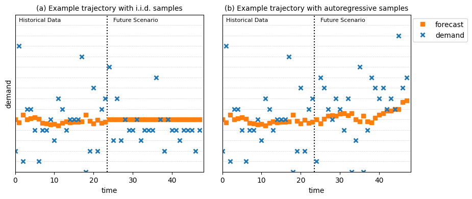
Figure 1: Example of demand trajectory range when drawing i.i.d. samples (a) vs. autoregressive samples (b).

However, knowing that companies employ forecasts and update those over time based on more recent observations, it is inconsistent to draw demand trajectory samples from stationary and i.i.d. distributions. Instead, to accurately represent reality when using solution methods like DRL, demand scenarios should be autoregressive, which would result in a different demand trajectory range, as illustrated in Figure 1 (b), which also reflects increasing demand uncertainty the longer we look into the future. With positive autocorrelation, if demand in early periods turns out higher than initially expected, then demand in later periods is likely to also be higher than initially anticipated. With negative autocorrelation, high demand in certain periods will be followed by periods with lower demand. That real-life demand processes are autoregressive is well-known. A celebrated approach to generate autoregressive time-series are ARIMA models (Hyndman  Athanasopoulos, 2018), and such models have also been studied in the context of demand modeling for inventory control (Graves, 1999; Gilbert, 2005).

The prevalence of autoregressive demand processes is also recognized by seminal books on inventory control (Silver ., 2017; Axsäter, 2015), which recommend forecasting via exponential smoothing as a suitable technique for most products. With this method, positive autocorrelation is the underlying assumption. Standard simple exponential smoothing yields point forecasts. While well-studied in forecasting literature, point forecasts are insufficient for properly balancing underage and overage costs in inventory control settings (Axsäter, 2015). For that latter purpose, estimating the standard deviation $\sigma$ as well as the mean $\mu$ of demand is crucial, and standard inventory textbooks (Silver ., 2017; Axsäter, 2015) recommend to estimate the second moment of demand by smoothing the forecast error over time, which yields an approach that we shall refer to as simple exponential smoothing for mean and standard deviation (SES). The forecasting literature has traditionally focused on point estimates, but the idea of forecasting variance has been proposed there as well, see e.g. Gelper . (2010).

The broad application of SES in inventory practice and recommendations by standard textbooks (Silver ., 2017; Axsäter, 2015) motivate us to study demand processes that are consistent with SES. Intuitively, this consistency entails that SES is a suitable forecasting process for the demand scenarios resulting from the demand generating process (DGP). That is, SES applied to the first $t$ data points $\{d_{1},...,d_{t}\}$ yields unbiased estimates of the mean and variance of the demand in period $t+1$. DGPs that are consistent with SES yield demand scenarios that are autoregressive.

For demand models to be practically useful, they would benefit from some properties in addition to being autoregressive. In particular, Kolassa (2016) and Rostami-Tabar  Disney (2023) emphasize the need for discrete, non-negative demand distributions in supply chain management, especially for low-volume demand, for example for safety stock setting, but also scenario analysis or other forecast-driven decision processes. Typical ARIMA models fall short in this regard: they tend to feature time series with continuous and negative values. More importantly, the error terms which cause the ‘shocks’ in the demand process are generally assumed to be independent, identically distributed variables (Graves, 1999; Gilbert, 2005), which is contrary to the idea of updating estimates of $\sigma$ over time.

When the demand can take on any real value, specifying a demand process that is consistent with any SES forecasting procedure is relatively straightforward, since for any combination of $\mu$ and $\sigma$ there exists a corresponding continuous distribution (for example a normal distribution). However, not all combinations of mean and variance have a corresponding distribution on the non-negative integers (see Adan ., 1995). A natural question that arises is whether there exist demand processes that are non-negative, discrete and consistent with SES forecasting.

In this paper, we answer this question, by deriving the conditions needed for existence of consistent demand processes on the non-negative integers. When these conditions are satisfied, the developments in this paper yield an intuitive and simple DGP that (1) is consistent with Simple Exponential Smoothing as proposed by the standard textbooks on inventory control (Axsäter (2015) and Silver . (2017)), (2) takes on values on the non-negative integers, and (3) considers updating the estimate of the demand variance rather than assuming known and exogenous variance (4) yields demand scenarios that are autoregressive, covering non-stationary developments of demand, such as exploding or vanishing demand trajectories, and (5) covers a variety of demand profiles (e.g. erratic or intermittent) as often seen in practice. The DGP can generate demand scenarios for any initial estimate of the mean and standard deviation of demand, and we view it as a key contribution of this paper.

To illustrate the relevance of the DGP, we demonstrate how these demand scenarios can be used in one specific type of supply chain operations planning problem: spare parts inventory control. Graves (1999) proposed a method for determining base-stock levels in case of non-stationary ARIMA demand. We evaluate the performance of that method in the context of the DGP studied in this paper. Additionally, we propose an alternative solution method that utilizes the knowledge about the DGP to determine base-stock levels that are better suited for these realistic low-volume demand processes.

The remainder of the paper is organized as follows: Section 2 provides an overview of the treatment of non-stationary demand processes for supply chain operations planning problems in literature. The DGP is proposed and analyzed in Section 3, where we also derive conditions under which the existence of the DGP can be guaranteed. In Section 4 we describe the application of our DGP in the context of a simple inventory control problem, propose the solution method for finding base-stock levels, and examine the performance of this solution method using numerical experiments. We conclude the paper in Section 5.

2 Literature review

The literature concerning demand processes can be roughly grouped into (1) stationary and independent and identically distributed (i.i.d.) demand and (2) non-stationary demand. Although i.i.d. stationary demand processes are popular because of their analytical tractability, they are often a poor reflection of reality. In this paper, we therefore focus on the body of literature for the latter category. Within non-stationary demand, we recognize two different streams of literature: (1) independent non-stationary demand and (2) autoregressive demand. Within the autoregressive demand stream, there are Markov-modulated and ARIMA-type demand processes. The contribution of this paper falls in the latter category.

While we aim to focus mostly on non-stationary demand, we call some attention to studies that investigate how best to forecast lead time demand variance for stationary demand processes. For example in inventory control problems, a common way of determining safety stock levels in practice is to assume that the demand follows a normal distribution, and then to multiply the lead time demand standard deviation with some safety factor to obtain a certain service level (Prak ., 2017). Note that for other types of distributions, it is possible to use the cumulative distribution function to find the value that corresponds to achieving a target service level. However, it is notoriously difficult to find the appropriate standard deviation of lead-time demand, even if the demand is stationary. The standard way of taking $\sigma\sqrt{L}$ as the standard deviation of lead-time demand ignores correlation of forecast errors and leads to an underestimation of the variance and thus safety stocks. Prak . (2017) and Janssen . (2009) demonstrate this and propose ways of correcting for this underestimation in stationary demand processes, in order to achieve the service level target.

In many papers considering non-stationary demand in operational planning problems, it is assumed that the demand distribution and its parameters are known, and independently varying over the periods in the time horizon. Xiang . (2018) compute near-optimal parameters of an ($s_{t},S_{t}$) lot sizing policy using mixed integer linear programming. The authors assume that the demand in a period follows a known probability density function. While they illustrate their results using a normal distribution, they argue that their modeling strategy is distribution independent. The coefficient of variation remains fixed in every time period, and the mean in each time period is given by some non-stationary pattern (e.g. a product life cycle pattern or sinusoidal oscillations). Furthermore, the distributions in each period are independent. Knowing that the majority of companies use time series forecasting methods to predict the demand over time, it is unlikely that demand in different periods is independent. There are a number of studies that employ similar ways of modeling the non-stationary demand when aiming to optimize lot sizing policy parameters, and the reader is referred to Ma . (2022) or Visentin . (2021) for an extensive overview of those papers.

Another way of modeling the fluctuating demand environment was proposed by Song  Zipkin (1993), where they consider that there are some identifiable factors (e.g. economic conditions, innovation) that determine the demand environment. This environment is modeled as a continuous-time Markov chain, and if the environment is in state $i$, demand follows a Poisson process with rate $\lambda_{i}$. This can be seen as an autoregressive demand process. With this generalization of standard demand processes, the authors provide qualitative descriptions of the forms of optimal inventory policies. Two algorithms are presented for computing the parameters of these policies. Other authors extend these Markov-modulated demand processes by investigating the impact of having partial observability of the demand (Bayraktar  Ludkovski, 2010), or demand correlations (Hu ., 2016) on the structure of the optimal policy. They find that in such cases, the optimal policy is a state-dependent ($s,S$) policy, which is promising as these are widely used in practice. However, finding the state-dependent parameters is not trivial, and analytically intractable.

Several authors have also addressed the issue of estimating the lead-time demand variance in non-stationary ARIMA-type processes. Graves (1999) models the demand as a (0,1,1) IMA process, where every period there is a shift in the mean of the demand process that is proportional (with factor $\alpha$) to the size of the shock which is normally distributed with mean $0$ and variance $\sigma^{2}$. Using this model for demand, the author provides a correction factor for the safety stock that is a function of the lead-time ($L$) and $\alpha$. Graves (1999) concludes that ‘we require dramatically more safety stock when demand is non-stationary, in comparison with the textbook case of stationary demand’ (p. 54). Strijbosch . (2011) use a similar model for the demand (the (0,1,1) ARIMA model), but they ensure that demand cannot be negative by truncating the mean. They conclude that most benefits in stock control performance can be attributed to having an appropriate demand variance updating procedure, rather than the choice of forecasting method or forecast parameter values. Prak  Teunter (2019) provide a framework on how to incorporate uncertainty about future demand into inventory models, using trended and random walk models for demand, that is normally distributed. Babai . (2022) explore three strategies to estimate variance of lead-time demand, and derive analytical results for an ARMA(1,1) demand process. Some research focuses on the need of predicting full lead-time demand distributions in supply chain operations planning. Cao  Shen (2019) propose a neural network model to forecast quantiles of a non-negative non-stationary autoregressive demand process.

A key feature of many autoregressive demand processes in literature is that they consider the variance of the underlying demand process to be exogenous and known. In practical settings, the variance of the demand is unknown and rather forecasted and updated based on demand observations, in line with the recommendations by seminal inventory control books (Axsäter, 2015; Silver ., 2017). Another feature of many studied autoregressive non-stationary models is that they are all considering real-valued demand, as opposed to discrete, integer-valued demand that is typically seen in practice. We contribute a DGP that addresses two gaps in literature: (1) the need for a practical discrete, non-negative, and non-stationary autoregressive stochastic process that (2) includes updating the forecast of the expectation as well as the demand variance as recommended by Axsäter (2015) and Silver . (2017). We contribute to literature by specifying a new demand process on the non-negative integers in which $\sigma$ is a forecast rather than an exogenously given number. In particular, $\sigma$ in our model is treated in the same way as the mean demand $\mu$: as an unknown parameter for which an initial estimate is available that will be updated in a manner consistent with Simple Exponential Smoothing (Axsäter, 2015; Silver ., 2017). We prove several desirable properties of the model, and illustrate a potential way in which it can be used to determine inventory control policies.

3 The demand generating process

Our proposed DGP is closely related to the exponential smoothing forecasting approach that shall be formalized in Section 3.1. The key ideas underlying the DGP will be introduced in Section 3.2, and some key analytical results are provided in Section 3.3. In Section 3.4 we reflect on the long term demand expectations of the proposed DGP.

3.1 Simple exponential smoothing

Simple exponential smoothing (SES) is a suitable forecasting approach when there is no clear trend or seasonality in demand. The DGP proposed in this paper is closely related to the SES forecasting method. To formally define SES, let $d_{1},d_{2},\ldots$ denote the demand time series, let $\alpha,\omega\in[0,1]$ denote two smoothing constants. Also, let $f_{t}$ and $MSE_{t}$ denote respectively our forecast of the mean demand in period $t$ and of the associated mean square error, based on all information available at time $t-1$. These forecasts are defined recursively by (see Silver ., 2017; Axsäter, 2015):

$$f_{t+1} =\alpha\cdot d_{t}+(1-\alpha)\cdot f_{t}$$ (1)

$$MSE_{t+1} =\omega\cdot(d_{t}-f_{t})^{2}+(1-\omega)\cdot MSE_{t}$$ (2)

Initial forecasts $f_{1}$ and $MSE_{1}$ can be obtained using any of the methods described in literature (Silver ., 2017; Axsäter, 2015). Note that in some versions of SES, only point forecasts are obtained via (1), but this is insufficient for applications in supply chain management, and hence we focus on SES as given by (1-2).

A DGP is a stochastic (demand) process $\{D_{t}\}_{t\in\mathbb{N}}$ from which realizations $d_{1},d_{2},\ldots,$ can be efficiently computed, e.g. for purposes of applying reinforcement learning, multi-stage stochastic programming, or bootstrapping. Suppose we would like to model a DGP for obtaining future demand scenarios for some product, and suppose that SES is an appropriate forecasting method for that product. This could very well be the case as SES is extensively applied in industry (Goltsos ., 2022) and recommended in seminal inventory textbooks. Then it is reasonable to suppose that SES could be successfully applied to the generated demand realizations, or, in other words, that the DGP is consistent with SES, in a sense to be defined next:

Definition 3.1.

Consider any DGP $\{D_{t}\}_{t\in\mathcal{N}}$, and consider the SES forecasting approach with given $\alpha$, $\omega$, and initial forecasts $f_{1}$, $MSE_{1}$. The DGP is consistent with the SES approach if (1-2) applied to the first $t$ data points $d_{1},...,d_{t}$ yields unbiased estimates $f_{t+1}$ and $MSE_{t+1}$ of the mean and variance of the (conditional) demand distribution $D_{t+1}$ in period $t+1$. That is, for any $t\in\mathbb{N}$:

$$\mu_{t+1} :=\mathbb{E}[D_{t+1}|D_{t}=d_{t},\ldots,D_{1}=d_{1}]=f_{t+1}$$ (3)

$$\sigma^{2}_{t+1} :=\mathbb{E}[(D_{t+1}-\mu_{t+1})^{2}|D_{t}=d_{t},\ldots,D_{1}=d_{1}]=MSE_{t+1}$$ (4)

With this definition in hand, we are ready to discuss our DGP.

3.2 Demand generating process

Consider any stochastic process $\{D_{t}\}_{t\in T}$ that is consistent with SES. Moreover, suppose that (given information on demand until $t$), $D_{t+1}$ is normally distributed. Since $\mathbb{E}[D_{1}]=\mu_{1}=f_{1}$ and $\mathbb{E}[(D_{1}-\mu_{1})^{2}]=\sigma_{1}^{2}=MSE_{1}$, the distribution of $D_{1}$ is fully specified. We may thus generate $d_{1}$, which in turn enables us to compute $f_{2}$ and $MSE_{2}$ using (1-2). Since $\mathbb{E}[D_{2}]=\mu_{2}=f_{2}$ and $\mathbb{E}[(D_{2}-\mu_{2})^{2}]=\sigma_{2}^{2}=MSE_{2}$, this in turn enables us to determine the distribution of $D_{2}$, which enables generation of $d_{2}$, etc.

Hence, under the assumption of normally distributed demands, it is relatively straightforward to obtain a DGP that is consistent with SES. However, since normal distributions are continuous and may take on negative values, this is typically not satisfactory for purposes of supply chain optimization, especially for low volume demand (see Sections 1 and 2). Instead, we would prefer to ensure that $D_{t}$ takes on values in the non-negative integers. For this purpose, we propose to adopt the fitting procedure suggested by Adan . (1995). Depending on the mean $\mu$ and variance $\sigma^{2}$, this procedure fits one in four classes of distributions defined on the non-negative integers. The distribution parameter $a$ ($a=\sigma^{2}/\mu^{2}-1/\mu$) determines which distribution class is to be fitted. In order of increasing variability, these classes are mixtures of binomials, Poisson, mixtures of negative-binomial and mixtures of geometric distributions with balanced means. Using this fitting procedure to obtain the distribution of $D_{t}$, instead of assuming normal distributions, yields the DGP that will be the subject of study for this paper.

This DGP may be used to generate sequences of discrete demands, based on an an initial estimate $f_{1},MSE_{1}$. The resulting demand sequences are autoregressive. As an illustration, Figure 2 shows two demand sequences obtained using the DGP, where in one demand sequence, the mean demand decreases, while in the other sequence the mean increases. Relatedly, if the initially provided estimate $\mu_{1}=f_{1}$ turns out to deviate considerably from $d_{1}$, then the uncertainty $MSE_{2}$ associated with $\mu_{2}$ is also revised upwards.

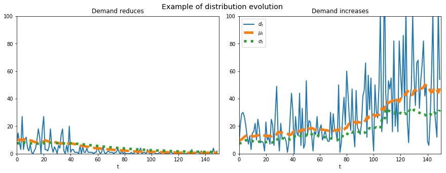
Figure 2: Example of two demand sequences having identical initial parameters ($f_{1}=10,MSE_{1}=60,\alpha=\omega=0.05$), and showing the evolution of $\mu_{t},\sigma_{t}$ over time.

A related and interesting feature of our proposed DGP is that the type of distribution may change when the forecast is updated over time, as the distribution parameter $a$ also changes over time as a result. This is shown in Figure 3 for the two example demand sequences of Figure 2. Note that for the demand sequence for which the mean decreases, the demand becomes intermittent, and the type of distribution that is fitted is more volatile (i.e., a geometric mixture distribution) than the original distribution that was based on initial estimates (i.e., a negative binomial mixture). In the case of increasing demand, the distribution class remains the same.

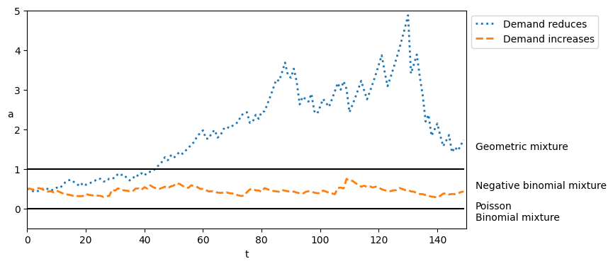
Figure 3: The evolution of distribution parameter $a=\frac{\sigma_{t}^{2}}{\mu_{t}^{2}}-\frac{1}{\mu_{t}}$ for the two demand sequences of Figure 2, showing the changing distribution type over time. $f_{1}=10,MSE_{1}=60,\alpha=\omega=0.05$

There is one caveat, however: it is well-known (see Adan ., 1995) that there does not exist a distribution on the non-negative integers for any combination of $\mu$ and $\sigma^{2}$; some combinations are not feasible. A relevant open question is then whether it is possible to define a consistent DGP on the non-negative integers.

To see why this question is relevant, suppose that $f_{1}=\mu_{1}$ and $MSE_{1}=\sigma^{2}_{1}$ represent a feasible combination, such that a discrete distribution can be fitted on $D_{1}$. This enables the generation of $d_{1}$, which yields $f_{2}=\mu_{2}$ and $MSE_{2}=\sigma^{2}_{2}$. But under which circumstances can we guarantee that $\mu_{2},\sigma^{2}_{2}$ is again feasible, etc., such that the sequence can be completed? The next section is devoted to answering this question.

3.3 Consistent DGPs on the non-negative integers

As discussed in the previous section, challenges may arise when attempting to define a consistent DGP on the non-negative integers. For instance, it is impossible to specify an integral distribution with mean 0.5 and variance less than 0.25. To ensure consistency with SES, our updates to the mean and variance of $D_{t}$ must follow (1) and (2), which may collide with the need to arrive at feasible combinations of $\mu_{t}$ and $\sigma_{t}^{2}$.

Theorem 3.2 demonstrates that such collisions can be avoided when $\alpha=\omega$. In Theorem 3.3 we show that when $\alpha\neq\omega$, feasibility cannot be guaranteed. Before presenting these theorems, we first present the next Lemma, which rephrases Lemma 2.1 of Adan . (1995):

Lemma 3.1.

For a pair of non-negative, real numbers ($\mu,\sigma^{2}$), there exists a corresponding random variable $X$ on the non-negative integers if and only if

$$\sigma^{2}\geq(\mu-\lfloor\mu\rfloor)(1-\mu+\lfloor\mu\rfloor)$$ (5)

implying that the variance of a distribution should be at least the variance of a binomial(1,$\mu-\lfloor\mu\rfloor$) distribution.

Proof.

Following Lemma 2.1 in Adan . (1995), let $k=\lfloor\mu\rfloor$. Let $\delta$ denote the difference between $k$ and $\mu$: $\delta=\mu-k=\mu-\lfloor\mu\rfloor$, meaning that $0\leq\delta<1$. We can rewrite $k=\mu-\delta$, and then we substitute $k$ in their Lemma 2.1:

$$\begin{split}\frac{\sigma^{2}}{\mu^{2}}&\geq\frac{2k+1}{\mu}-\frac{k(k+1)}{\mu^{2}}-1\\ &\geq\frac{2(\mu-\delta)+1}{\mu}-\frac{(\mu-\delta)(\mu-\delta+1)}{\mu^{2}}-1\\ &\geq\frac{2\mu-2\delta+1}{\mu}-\frac{\mu^{2}-2\delta\mu+\mu-\delta+\delta^{2}}{\mu^{2}}-1\\ &\geq\left(\frac{2\mu}{\mu}-\frac{2\delta}{\mu}+\frac{1}{\mu}\right)-\left(\frac{\mu^{2}}{\mu^{2}}-\frac{2\mu\delta}{\mu^{2}}+\frac{\mu}{\mu^{2}}+\frac{\delta^{2}}{\mu^{2}}-\frac{\delta}{\mu^{2}}\right)-1\\ &\geq 2-\frac{2\delta}{\mu}+\frac{1}{\mu}-1+\frac{2\delta}{\mu}-\frac{1}{\mu}-\frac{\delta^{2}}{\mu^{2}}+\frac{\delta}{\mu^{2}}-1\\ &\geq-\frac{\delta^{2}}{\mu^{2}}+\frac{\delta}{\mu^{2}}\\ &\geq\frac{\delta(1-\delta)}{\mu^{2}}\\ \sigma^{2}&\geq\delta(1-\delta)=(\mu-\lfloor\mu\rfloor)(1-\mu+\lfloor\mu\rfloor)\\ \end{split}$$ (6)

∎

We are now ready to prove the main result of this section:

Theorem 3.2.

Let $\{D_{t}\}_{t\in\mathbb{N}}$ be a stochastic demand process on the non-negative integer domain, and suppose that $(\mu_{1},\sigma_{1}^{2})$ satisfies feasibility condition (5). Given $d_{1},\ldots,d_{t}$, let $\mu_{t}=f_{t}$, $\sigma_{t}^{2}=MSE_{t}$ be defined as in (1-2), using smoothing parameters $\alpha$ and $\omega=\alpha$. Then the resulting combination ($\mu_{t}$, $\sigma^{2}_{t}$) satisfies feasibility condition (5), and may hence be used to fit a new non-negative integer distribution.

Whereas the stochastic demand process remains feasible to fit a non-negative integer distribution when using $\alpha=\omega$, this feasibility cannot be guaranteed if $\alpha\neq\omega$, as shown in Theorem 3.3.

Theorem 3.3.

Let $\{D_{t}\}_{t\in\mathbb{N}}$ be a stochastic demand process on the non-negative integer domain, and suppose that $(\mu_{1},\sigma_{1}^{2})$ satisfies feasibility condition (5). Given $d_{1},\ldots,d_{t}$, let $\mu_{t}=f_{t}$, $\sigma_{t}^{2}=MSE_{t}$ be defined as in (1-2), using smoothing parameters $\alpha$ and $\omega\neq\alpha$. Then the resulting combination ($\mu_{t}$, $\sigma^{2}_{t}$) is not guaranteed to satisfy feasibility condition (5), and with positive probability it cannot be used to fit a new non-negative integer distribution.

Proof.

We prove that we cannot guarantee feasibility of the resulting combination of $\mu_{t+1}$ and $\sigma_{t+1}$ for $\alpha\neq\omega$ by giving a counterexample that shows that feasibility condition (5) no longer holds. In the counterexample we have a $Bin(1,p)$ distribution at time $t$, with $\mu_{t}=p$ and $\sigma_{t}^{2}=p(1-p)$. Suppose we use smoothing constants $\alpha$ and $\omega$ and that we draw $d_{t}=0$. The updated values are now (7) and (8).

$$\mu_{t+1}=(1-\alpha)\mu_{t}+\alpha d_{t}=(1-\alpha)p$$ (7)

$$\sigma_{t+1}^{2}=(1-\omega)\sigma_{t}^{2}+\omega(d_{t}-\mu_{t})^{2}=(1-\omega)p(1-p)+\omega p^{2}$$ (8)

Note that in this binomial distribution, $\delta_{t+1}=\mu_{t+1}$. To fit a feasible non-negative integer distribution, feasibility condition (5) must hold. We find using (9) that it could also be that $\sigma_{t+1}^{2}-\mu_{t+1}(1-\mu_{t+1})<0$ when using $\alpha\neq\omega$, as $(p-2p^{2})$ can take positive values as well as negative values.

$$\begin{split}\sigma_{t+1}^{2}-\mu_{t+1}(1-\mu_{t+1})&=(1-\omega)p(1-p)+\omega p^{2}-(1-\alpha)p(1-(1-\alpha)p)\\ &=p-p\omega-p^{2}+2\omega p^{2}-(p-p^{2}+2\alpha p^{2}-\alpha p-\alpha^{2}p^{2})\\ &=\alpha^{2}p^{2}+2\omega p^{2}-2\alpha p^{2}+\alpha p-\omega p\\ &=(\alpha p)^{2}+(\alpha-\omega)(p-2p^{2})\\ \end{split}$$ (9)

In that case feasibility condition (5) does not hold, and there is no feasible non-negative integer distribution for that combination of $\mu_{t+1}$ and $\sigma_{t+1}$, thus completing our counterexample. ∎

We have now shown the necessary condition for which we can define a consistent DGP on the non-negative integers: one needs to use identical smoothing parameters for the mean and variance (1-2).

3.4 Longer term demand estimates

In this section, we make a few observations regarding the longer-term one-step-ahead demand expectations in the proposed DGP. As illustrated in Figure 2, the DGP may yield individual demand realizations that, over time, deviate substantially from $f_{1}=\mu_{1}$ in either direction. One may wonder whether over the longer term, demand realizations from the DGP are expected to be higher or lower compared to the initial estimate. When utilizing the different demand samples in a method such as DRL, it is desirable if on average they remain in line with the initial forecast, i.e. they are unbiased. In fact, since $\mu_{t}$ is known, based on $d_{1},\ldots,d_{t-1}$, we may observe the following:

$$\begin{split}\mathbb{E}[D_{t+1}]=\mathbb{E}[\mathbb{E}[f_{t+1}|f_{t}]]&=\mathbb{E}[(1-\alpha)\cdot\mathop{\mathbb{E}}[f_{t}|f_{t}]+\alpha\cdot\mathop{\mathbb{E}}[{d_{t}}|f_{t}]]\\ &=\mathbb{E}[(1-\alpha)\cdot f_{t}+\alpha\cdot f_{t}]\\ &=\mathbb{E}[f_{t}]=\mathbb{E}[D_{t}]=f_{1}\end{split}$$ (10)

Here, the first equality follows from (1), the second equality holds because $f_{t}=\mu_{t}$, and the last equality holds by continuing this type of argument recursively. Thus, over time, the expectation of the mean of the DGP remains the same as the initial estimate of the mean $f_{1}$. A similar identity can be derived for the expected variance:

$$\begin{split}\mathbb{E}[MSE_{t+1}]=\mathbb{E}[\mathbb{E}[MSE_{t+1}|MSE_{t}]]&=\mathbb{E}[(1-\omega)\cdot\mathbb{E}[MSE_{t}]+\omega\cdot\mathbb{E}[(d_{t}-f_{t})^{2}]]\\ &=\mathbb{E}[(1-\omega)\cdot\mathbb{E}[MSE_{t}]+\omega\cdot\mathbb{E}[MSE_{t}]]\\ &=\mathbb{E}[MSE_{t}]=\mathbb{E}[\sigma_{t}^{2}]=MSE_{1}\end{split}$$ (11)

Here, we observe that the parameter $MSE_{t}$ that represents the estimated one-step-ahead variance remains in expectation equal to the initial estimate of the one-step-ahead variance $MSE_{1}$.

In fact, using an ARIMA process for generating non-negative integer demand trajectories does not exhibit this lack of bias. If one were to use the (0,1,1) ARIMA process to generate demand observations, truncate negative values, and round the continuous values to the nearest integer, the average demand in the long-term would deviate significantly from the initial forecast, as shown in Figure 4. While the ARIMA process would generally yield unbiased trajectories in cases with a very low coefficient of variation, once the standard deviation is in a similar magnitude of the mean, a lot of bias is introduced. This highlights the importance of having an appropriate DGP for non-negative integer distributions.

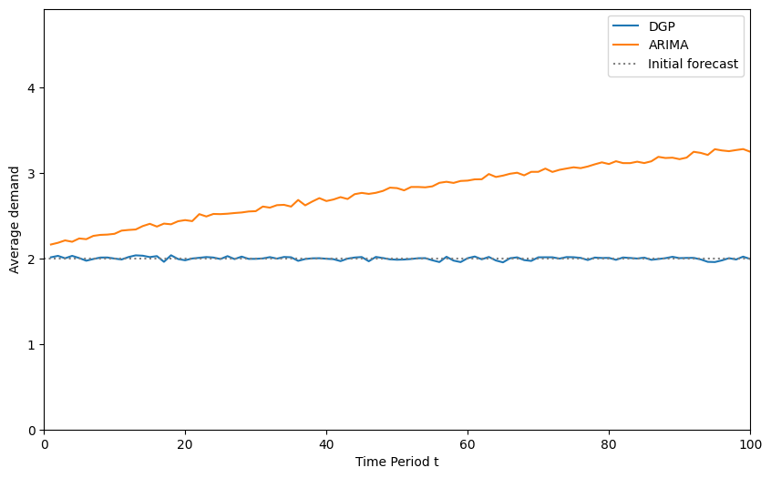
Figure 4: The average value of 10,000 demand samples at increasing time periods $t$. In this case the initial forecast is equal to 2, the standard deviation $\sigma=2$, smoothing parameter $\alpha=0.1$. Using the ARIMA process to generate demand introduces bias, while the DGP proposed in this paper remains unbiased.

4 Application in inventory control

To illustrate a potential application of the DGP as described in Section 3, we consider an inventory control problem with low volume demand. It is a common problem in industry, for example when considering spare parts inventory. In this problem we have an inventory system where we have to replenish products with non-stationary stochastic demand, such that we are able to meet customer demand immediately from stock. Replenishment orders are delivered after a deterministic lead time ($l$). At the beginning of a period, we have to place a replenishment order. This becomes available after $l$ periods. After placing an order, we observe and satisfy demand. This means that there are $l+1$ periods of uncertain demand to cover before the replenishment order becomes available. Any demand that cannot be satisfied is backordered. The inventory transition function that describes how demand, backorders, inventory and replenishment orders relate to each other is defined by (12), with a summary of the notation shown in Table LABEL:table:modelnotation. Backorders are fulfilled first, followed by any new demand in the period (13). The costs per period are either inventory holding costs or backorder penalty costs (14).

$$I_{t-1}-b_{t-1}+q_{t}=d_{t}+I_{t}-b_{t}$$ (12)

$$d_{t}^{s}=\min(I_{t-1}-b_{t-1}+q_{t},d_{t})$$ (13)

$$c_{t}=h\cdot I_{t}+p\cdot b_{t}$$ (14)

We evaluate how existing solution methods for the inventory control problem perform when encountering low volume and highly variable demand, which follows our proposed DGP. Additionally we provide a new solution method that uses some information about the DGP. We describe these solution methods in section 4.1. The setup of numerical experiments to evaluate the performance of these solution methods is specified in section 4.2. Finally, the results of these numerical experiments are presented in section 4.3.

4.1 Solution methods

A typical approach to solving the inventory control problem is to follow a base-stock policy. In this policy, we need to set a base-stock level $S_{t}$ that covers the demand during lead-time plus some uncertainty. Every period, the replenishment order is equal to the base-stock level minus the current inventory position ($q_{t+l}=S_{t}-IP_{t}$), if the inventory position (15) is below $S_{t}$.

$$IP_{t}=I_{t-1}-b_{t-1}+\sum_{t^{\prime}=t}^{t+L-1}q_{t^{\prime}}$$ (15)

Several authors have found that a state-dependent $(s,S)$-policy is optimal for this problem (see Section 2) when there is Markov-modulated non-stationary demand. In our case of autoregressive non-stationary demand, such an optimal structure has not been proven, although a policy of that structure is very common to use. In any case, it still remains difficult to find the optimal base-stock levels. However, there are some well-established guidelines in determining the parameters, namely to set the base-stock with a certain service level target in mind.

There are different kinds of service level targets under consideration in inventory control problems. Often in literature, the ‘in-stock probability’ ($P_{1}$-service level) is used (16), which is the probability of not observing a stock-out during the lead time. Another service level is the fill rate ($P_{2}$-service level), which is the proportion of demand that is met during lead time (17). Typically, when computing the base-stock level the ‘in-stock probability’ target is considered, mainly for its prevalence in common textbooks and ease of use with regards to its implementation with cumulative distribution functions.

$$\hat{P_{1}}=\frac{1}{T}\sum_{t\in T}P(I_{t-1}-b_{t-1}+q_{t}\geq d_{t})$$ (16)

$$\hat{P_{2}}=\sum_{t\in T}\frac{d_{t}^{s}}{d_{t}}$$ (17)

When considering an in-stock probability target $P_{1}^{*}$, the base-stock level can be computed by $S=L\mu+\phi(P_{1}^{*})\sigma\sqrt{L}$. A key assumption in this method is that the demand follows a (stationary) normal distribution that is i.i.d. over time, which makes the cumulative distribution function (CDF) for the standard normal random variable $\phi(P_{1}^{*})$ applicable. Note that since we have a periodic review of the inventory (every period), the lead time that we need to consider in the base-stock level calculations is the sum of the lead time and review period ($L=l+1$). In cases that a different demand distribution is assumed, the CDF is required to determine the base-stock level. In the experiments, we use the CDF of the standard normal random variable.

The standard deviation of demand is often linked to the forecast error, and Prak . (2017) show that even with stationary demand, the forecast errors over the lead time demand are positively correlated. Without considering that correlation, the standard deviation of demand is often underestimated and needs to be corrected. The standard deviation may need additional corrections due to the non-stationarity of demand.

Solution method 1 (S1)

Graves (1999) provides a correction factor in the case that demand follows an ARIMA process that is forecasted with single exponential smoothing (18) with parameter $\alpha$. This indicates that the standard deviation should be inflated due to the additional uncertainty in the demand process.

$$S_{ses}=L\mu+\phi(P_{1}^{*})\sigma\sqrt{L}\sqrt{1+\alpha(L-1)+\alpha^{2}\frac{(L-1)(2L-1)}{6}}$$ (18)

We consider two variants of this solution method. Commonly the estimate for $\mu$ is updated in ARIMA processes, while the estimate for $\sigma$ is considered to stay unchanged (S1a). The impact of using updated estimates of $\sigma$ in (18) is studied (S1b). Note that in Graves’ model, the demand is real-valued and can take on negative values. This could lead to underestimating the base-stock level that is needed when demand is integer-valued and non-negative, especially in cases similar to the example in Figure 4.

Solution method 2 (S2)

Using the DGP proposed in this paper, we can generate non-negative and integer-valued demand scenarios. With these scenarios, we can derive an empirical CDF, which we then use to find the base-stock level (19).

$$S_{emp}=\hat{F_{n}}(P_{1}^{*})$$ (19)

The empirical CDF is found as follows:

1. Generate $n=10,000$ demand scenarios of length $L$, given an initial estimate for $\mu$ and $\sigma$

2. Compute lead time demand for each scenario: $\sum_{t=0}^{L}d_{t}$

3. Compute empirical CDF based on the $n$ lead time demand observations and target in-stock probability

4.2 Experimental setup

To evaluate the performance of the two solution methods for computing the base-stock level in low-volume spare parts environment, we consider a number of different problem parameters. For the DGP, we consider two different cases of low volume demand, that have a highly variable initial starting distributions as given by the paper of Adan . (1995). We investigate three different values for the smoothing parameter. Note that 0.1 is recommended as a maximum value as by Silver . (2017). Especially in cases with longer lead times, the empirical variance of lead time demand could be very different from the normal distribution or ARIMA approximations. Therefore we consider several levels of the lead time $l$. We also consider several levels of the penalty costs $p$, which are used to compute the in-stock probability target ($P_{1}^{*}=\frac{p}{p+h}$). We look at the target in-stock probabilities to identify the efficiency curve (trade off between inventory and fill rate). A summary of the experimental settings is found in Table LABEL:table:experimental-settings.

To evaluate the performance of the three solution methods, we run 10,000 simulations for 100 time periods each. The demand in the simulation is based on the DGP described in section 3, generated with $\alpha$. At period 1, there is no starting inventory, and we use $2\cdot L$ periods as warm-up periods. We are interested in the performance of the different methods on the expected costs per period ($\mathbb{E}[c_{t}]$) and their achieved fill rate (17) combined with average on hand inventory levels. Note that in setting the base-stock level, the in-stock probability target is considered. Nevertheless, the fill rate is a more common service measure in practice as it considers the magnitude of not satisfying demand as well. Small cases of lost demand are less damaging than in case of the in-stock probability, but missing large demand has a heavier impact on the fill rate. That is why we focus on the fill rate performance in the next section.

4.3 Results

5 Conclusion

We proposed a new demand process for non-stationary demand that is useful in generating practical and realistic demand scenarios. In this DGP, the expectation and variance of demand are treated as a forecast rather than an exogenously given number. This is in line with recommendations in seminal literature (Axsäter, 2015; Silver ., 2017). Additionally, this DGP generates non-negative integer demand, using a powerful fitting technique proposed by Adan . (1995). We proved the conditions under which this DGP is feasible, and demonstrated that the model is able to generate realistic and practically relevant demand scenarios.

Subsequently, we investigated a spare parts inventory control problem in this non-stationary demand setting using the DGP to generate the evaluation scenarios. We evaluated two existing base-stock policies, and suggested a new base-stock level computation method that utilizes the DGP to find an empirical CDF of demand during lead time, and then sets appropriate base-stock levels, outperforming existing base-stock policies. In cases these cases of low-volume demand, where the degree of non-stationarity is high, the variance is high and lead times are long, the method of Graves (1999), which considers potentially negative and continuous demand, leads to underestimations of the heavy tail of the demand distribution. The newly suggested method is better able to estimate the heavy tail of the demand distribution, an essential ingredient for finding appropriate inventory control parameters.

The characteristics and properties of the DGP in this paper can be utilized in more ways to specify and evaluate new inventory control policies for non-stationary demand settings. In addition to the inventory control problem, other supply chain operations planning problems could also be studied using the DGP in this paper. Another direction for future research is to study how trend and seasonality can also be incorporated in the DGP, as these will increase the practical relevance of the DGP even further. A final interesting future research direction is to understand how these non-stationary demand scenarios impact results found in optimization algorithms like multi-stage stochastic programming or Deep Reinforcement Learning. The non-stationarity of the scenarios could pose extra challenges to these algorithms, which requires additional research.

References

- Adan \BOthers. (\APACyear1995) \APACinsertmetastarAdan1995{APACrefauthors}Adan, I., van Eenige, M.\BCBL \BBA Resing, J. \APACrefYearMonthDay1995. \BBOQ\APACrefatitleFitting discrete distributions on the first two moments Fitting discrete distributions on the first two moments.\BBCQ \APACjournalVolNumPagesProbability in the engineering and informational sciences94623–632. \PrintBackRefs\CurrentBib
- Altendorfer \BOthers. (\APACyear2016) \APACinsertmetastarAltendorfer2016{APACrefauthors}Altendorfer, K., Felberbauer, T.\BCBL \BBA Jodlbauer, H. \APACrefYearMonthDay2016. \BBOQ\APACrefatitleEffects of forecast errors on optimal utilisation in aggregate production planning with stochastic customer demand Effects of forecast errors on optimal utilisation in aggregate production planning with stochastic customer demand.\BBCQ \APACjournalVolNumPagesInternational Journal of Production Research543718-3735. {APACrefURL} http://dx.doi.org/10.1080/00207543.2016.1162918 {APACrefDOI} \doi10.1080/00207543.2016.1162918 \PrintBackRefs\CurrentBib
- Axsäter (\APACyear2015) \APACinsertmetastarAxsater2015{APACrefauthors}Axsäter, S. \APACrefYearMonthDay2015. \BBOQ\APACrefatitleForecasting Forecasting.\BBCQ \BIn \APACrefbtitleInventory Control Inventory control (\PrintOrdinalThird Edit \BEd, \BPGS 7–36). \APACaddressPublisherSpringer. \PrintBackRefs\CurrentBib
- Babai \BOthers. (\APACyear2022) \APACinsertmetastarZiedBabai2022{APACrefauthors}Babai, M\BPBIZ., Dai, Y., Li, Q., Syntetos, A.\BCBL \BBA Wang, X. \APACrefYearMonthDay2022. \BBOQ\APACrefatitleForecasting of lead-time demand variance: Implications for safety stock calculations Forecasting of lead-time demand variance: Implications for safety stock calculations.\BBCQ \APACjournalVolNumPagesEuropean Journal of Operational Research2963846–861. {APACrefURL} https://doi.org/10.1016/j.ejor.2021.04.017 {APACrefDOI} \doi10.1016/j.ejor.2021.04.017 \PrintBackRefs\CurrentBib
- Bayraktar \BBA Ludkovski (\APACyear2010) \APACinsertmetastarBayraktar2010{APACrefauthors}Bayraktar, E.\BCBT \BBA Ludkovski, M. \APACrefYearMonthDay2010. \BBOQ\APACrefatitleInventory management with partially observed nonstationary demand Inventory management with partially observed nonstationary demand.\BBCQ \APACjournalVolNumPagesAnnals of Operations Research17617–39. {APACrefDOI} \doi10.1007/s10479-009-0513-8 \PrintBackRefs\CurrentBib
- Bertsimas \BOthers. (\APACyear2019) \APACinsertmetastarBertsimas2019{APACrefauthors}Bertsimas, D., Sim, M.\BCBL \BBA Zhang, M. \APACrefYearMonthDay2019. \BBOQ\APACrefatitleAdaptive distributionally robust optimization Adaptive distributionally robust optimization.\BBCQ \APACjournalVolNumPagesManagement Science652604–618. {APACrefDOI} \doi10.1287/mnsc.2017.2952 \PrintBackRefs\CurrentBib
- Boute \BOthers. (\APACyear2022) \APACinsertmetastarboute2022deep{APACrefauthors}Boute, R\BPBIN., Gijsbrechts, J., Van Jaarsveld, W.\BCBL \BBA Vanvuchelen, N. \APACrefYearMonthDay2022. \BBOQ\APACrefatitleDeep reinforcement learning for inventory control: A roadmap Deep reinforcement learning for inventory control: A roadmap.\BBCQ \APACjournalVolNumPagesEuropean Journal of Operational Research2982401–412. \PrintBackRefs\CurrentBib
- Boylan \BBA Babai (\APACyear2022) \APACinsertmetastarBoylan2022{APACrefauthors}Boylan, J\BPBIE.\BCBT \BBA Babai, M\BPBIZ. \APACrefYearMonthDay2022. \BBOQ\APACrefatitleEstimating the cumulative distribution function of lead-time demand using bootstrapping with and without replacement Estimating the cumulative distribution function of lead-time demand using bootstrapping with and without replacement.\BBCQ \APACjournalVolNumPagesInternational Journal of Production Economics252April108586. {APACrefURL} https://doi.org/10.1016/j.ijpe.2022.108586 {APACrefDOI} \doi10.1016/j.ijpe.2022.108586 \PrintBackRefs\CurrentBib
- Cao \BBA Shen (\APACyear2019) \APACinsertmetastarCao2019{APACrefauthors}Cao, Y.\BCBT \BBA Shen, Z\BPBIJ\BPBIM. \APACrefYearMonthDay2019. \BBOQ\APACrefatitleQuantile forecasting and data-driven inventory management under nonstationary demand Quantile forecasting and data-driven inventory management under nonstationary demand.\BBCQ \APACjournalVolNumPagesOperations Research Letters476465–472. {APACrefURL} https://doi.org/10.1016/j.orl.2019.08.008 {APACrefDOI} \doi10.1016/j.orl.2019.08.008 \PrintBackRefs\CurrentBib
- Gelper \BOthers. (\APACyear2010) \APACinsertmetastarGelper2010{APACrefauthors}Gelper, S., Fried, R.\BCBL \BBA Croux, C. \APACrefYearMonthDay2010. \BBOQ\APACrefatitleRobust forecasting with exponential and holt-winters smoothing Robust forecasting with exponential and holt-winters smoothing.\BBCQ \APACjournalVolNumPagesJournal of Forecasting293285–300. {APACrefDOI} \doi10.1002/for.1125 \PrintBackRefs\CurrentBib
- Gilbert (\APACyear2005) \APACinsertmetastarGilbert2005{APACrefauthors}Gilbert, K. \APACrefYearMonthDay2005. \BBOQ\APACrefatitleAn ARIMA supply chain model An ARIMA supply chain model.\BBCQ \APACjournalVolNumPagesManagement Science512305–310. {APACrefDOI} \doi10.1287/mnsc.1040.0308 \PrintBackRefs\CurrentBib
- Goltsos \BOthers. (\APACyear2022) \APACinsertmetastarGoltsos2022{APACrefauthors}Goltsos, T\BPBIE., Syntetos, A\BPBIA., Glock, C\BPBIH.\BCBL \BBA Ioannou, G. \APACrefYearMonthDay2022. \BBOQ\APACrefatitleInventory – forecasting: Mind the gap Inventory – forecasting: Mind the gap.\BBCQ \APACjournalVolNumPagesEuropean Journal of Operational Research2992397–419. {APACrefURL} https://doi.org/10.1016/j.ejor.2021.07.040 {APACrefDOI} \doi10.1016/j.ejor.2021.07.040 \PrintBackRefs\CurrentBib
- Graves (\APACyear1999) \APACinsertmetastarGraves1999{APACrefauthors}Graves, S\BPBIC. \APACrefYearMonthDay1999. \BBOQ\APACrefatitleA Single-Item Inventory Model for a Nonstationary Demand Process A Single-Item Inventory Model for a Nonstationary Demand Process.\BBCQ \APACjournalVolNumPagesManufacturing & Service Operations Management1150–61. {APACrefDOI} \doi10.1287/msom.1.2.174 \PrintBackRefs\CurrentBib
- Hu \BOthers. (\APACyear2016) \APACinsertmetastarHu2016{APACrefauthors}Hu, J., Zhang, C.\BCBL \BBA Zhu, C. \APACrefYearMonthDay2016. \BBOQ\APACrefatitle(s, S) Inventory systems with correlated demands (s, S) Inventory systems with correlated demands.\BBCQ \APACjournalVolNumPagesINFORMS Journal on Computing284603–611. \PrintBackRefs\CurrentBib
- Hyndman \BBA Athanasopoulos (\APACyear2018) \APACinsertmetastarhyndman2018forecasting{APACrefauthors}Hyndman, R\BPBIJ.\BCBT \BBA Athanasopoulos, G. \APACrefYear2018. \APACrefbtitleForecasting: principles and practice Forecasting: principles and practice. \APACaddressPublisherOTexts. \PrintBackRefs\CurrentBib
- Janssen \BOthers. (\APACyear2009) \APACinsertmetastarJanssen2009{APACrefauthors}Janssen, E., Strijbosch, L.\BCBL \BBA Brekelmans, R. \APACrefYearMonthDay2009. \BBOQ\APACrefatitleAssessing the effects of using demand parameters estimates in inventory control and improving the performance using a correction function Assessing the effects of using demand parameters estimates in inventory control and improving the performance using a correction function.\BBCQ \APACjournalVolNumPagesInternational Journal of Production Economics118134–42. {APACrefDOI} \doi10.1016/j.ijpe.2008.08.029 \PrintBackRefs\CurrentBib
- Kataoka (\APACyear1963) \APACinsertmetastarkataoka1963stochastic{APACrefauthors}Kataoka, S. \APACrefYearMonthDay1963. \BBOQ\APACrefatitleA stochastic programming model A stochastic programming model.\BBCQ \APACjournalVolNumPagesEconometrica: Journal of the Econometric Society181–196. \PrintBackRefs\CurrentBib
- Kolassa (\APACyear2016) \APACinsertmetastarKolassa2016{APACrefauthors}Kolassa, S. \APACrefYearMonthDay2016. \BBOQ\APACrefatitleEvaluating predictive count data distributions in retail sales forecasting Evaluating predictive count data distributions in retail sales forecasting.\BBCQ \APACjournalVolNumPagesInternational Journal of Forecasting323788–803. {APACrefURL} http://dx.doi.org/10.1016/j.ijforecast.2015.12.004 {APACrefDOI} \doi10.1016/j.ijforecast.2015.12.004 \PrintBackRefs\CurrentBib
- Ma \BOthers. (\APACyear2022) \APACinsertmetastarMa2022{APACrefauthors}Ma, X., Rossi, R.\BCBL \BBA Archibald, T\BPBIW. \APACrefYearMonthDay2022. \BBOQ\APACrefatitleApproximations for non-stationary stochastic lot-sizing under (s,Q)-type policy Approximations for non-stationary stochastic lot-sizing under (s,Q)-type policy.\BBCQ \APACjournalVolNumPagesEuropean Journal of Operational Research2982573–584. {APACrefURL} https://doi.org/10.1016/j.ejor.2021.06.013 {APACrefDOI} \doi10.1016/j.ejor.2021.06.013 \PrintBackRefs\CurrentBib
- Prak \BBA Teunter (\APACyear2019) \APACinsertmetastarPrak2019{APACrefauthors}Prak, D.\BCBT \BBA Teunter, R. \APACrefYearMonthDay2019. \BBOQ\APACrefatitleA general method for addressing forecasting uncertainty in inventory models A general method for addressing forecasting uncertainty in inventory models.\BBCQ \APACjournalVolNumPagesInternational Journal of Forecasting351224–238. {APACrefURL} https://doi.org/10.1016/j.ijforecast.2017.11.004 {APACrefDOI} \doi10.1016/j.ijforecast.2017.11.004 \PrintBackRefs\CurrentBib
- Prak \BOthers. (\APACyear2017) \APACinsertmetastarPrak2017{APACrefauthors}Prak, D., Teunter, R.\BCBL \BBA Syntetos, A. \APACrefYearMonthDay2017. \BBOQ\APACrefatitleOn the calculation of safety stocks when demand is forecasted On the calculation of safety stocks when demand is forecasted.\BBCQ \APACjournalVolNumPagesEuropean Journal of Operational Research2562454–461. {APACrefURL} http://dx.doi.org/10.1016/j.ejor.2016.06.035 {APACrefDOI} \doi10.1016/j.ejor.2016.06.035 \PrintBackRefs\CurrentBib
- Rostami-Tabar \BBA Disney (\APACyear2023) \APACinsertmetastarRostami-Tabar2023{APACrefauthors}Rostami-Tabar, B.\BCBT \BBA Disney, S\BPBIM. \APACrefYearMonthDay2023. \BBOQ\APACrefatitleOn the order-up-to policy with intermittent integer demand and logically consistent forecasts On the order-up-to policy with intermittent integer demand and logically consistent forecasts.\BBCQ \APACjournalVolNumPagesInternational Journal of Production Economics257December 2022108763. {APACrefURL} https://doi.org/10.1016/j.ijpe.2022.108763 {APACrefDOI} \doi10.1016/j.ijpe.2022.108763 \PrintBackRefs\CurrentBib
- Silver \BOthers. (\APACyear2017) \APACinsertmetastarSilver2017{APACrefauthors}Silver, E\BPBIA., Pyke, D\BPBIF.\BCBL \BBA Thomas, D\BPBIJ. \APACrefYearMonthDay2017. \BBOQ\APACrefatitleForecasting Models and Techniques Forecasting Models and Techniques.\BBCQ \BIn \APACrefbtitleInventory and Production Management in Supply Chains Inventory and production management in supply chains (\PrintOrdinalFourth Edition \BEd, \BPGS 73–144). \APACaddressPublisherTaylor & Francis Group. \PrintBackRefs\CurrentBib
- Snyder \BOthers. (\APACyear2002) \APACinsertmetastarSnyder2002{APACrefauthors}Snyder, R\BPBID., Koehler, A\BPBIB.\BCBL \BBA Ord, J\BPBIK. \APACrefYearMonthDay2002. \BBOQ\APACrefatitleForecasting for inventory control with exponential smoothing Forecasting for inventory control with exponential smoothing.\BBCQ \APACjournalVolNumPagesInternational Journal of Forecasting1815–18. {APACrefDOI} \doi10.1016/S0169-2070(01)00109-1 \PrintBackRefs\CurrentBib
- Song \BBA Zipkin (\APACyear1993) \APACinsertmetastarSong1993{APACrefauthors}Song, J\BHBIs.\BCBT \BBA Zipkin, P. \APACrefYearMonthDay1993. \BBOQ\APACrefatitleInventory Control in a Fluctuating Demand Environment Inventory Control in a Fluctuating Demand Environment.\BBCQ \APACjournalVolNumPagesOperations Research412351–370. \PrintBackRefs\CurrentBib
- Strijbosch \BOthers. (\APACyear2011) \APACinsertmetastarStrijbosch2011{APACrefauthors}Strijbosch, L\BPBIW., Syntetos, A\BPBIA., Boylan, J\BPBIE.\BCBL \BBA Janssen, E. \APACrefYearMonthDay2011. \BBOQ\APACrefatitleOn the interaction between forecasting and stock control: The case of non-stationary demand On the interaction between forecasting and stock control: The case of non-stationary demand.\BBCQ \APACjournalVolNumPagesInternational Journal of Production Economics1331470–480. {APACrefURL} http://dx.doi.org/10.1016/j.ijpe.2009.10.032 {APACrefDOI} \doi10.1016/j.ijpe.2009.10.032 \PrintBackRefs\CurrentBib
- Visentin \BOthers. (\APACyear2021) \APACinsertmetastarVisentin2021{APACrefauthors}Visentin, A., Prestwich, S., Rossi, R.\BCBL \BBA Tarim, S\BPBIA. \APACrefYearMonthDay2021. \BBOQ\APACrefatitleComputing optimal (R, s, S) policy parameters by a hybrid of branch-and-bound and stochastic dynamic programming Computing optimal (R, s, S) policy parameters by a hybrid of branch-and-bound and stochastic dynamic programming.\BBCQ \APACjournalVolNumPagesEuropean Journal of Operational Research294191–99. {APACrefURL} https://doi.org/10.1016/j.ejor.2021.01.012 {APACrefDOI} \doi10.1016/j.ejor.2021.01.012 \PrintBackRefs\CurrentBib
- Xiang \BOthers. (\APACyear2018) \APACinsertmetastarXiang2018{APACrefauthors}Xiang, M., Rossi, R., Martin-Barragan, B.\BCBL \BBA Tarim, S\BPBIA. \APACrefYearMonthDay2018. \BBOQ\APACrefatitleComputing non-stationary (s, S) policies using mixed integer linear programming Computing non-stationary (s, S) policies using mixed integer linear programming.\BBCQ \APACjournalVolNumPagesEuropean Journal of Operational Research2712490–500. {APACrefURL} https://doi.org/10.1016/j.ejor.2018.05.030 {APACrefDOI} \doi10.1016/j.ejor.2018.05.030 \PrintBackRefs\CurrentBib