Active flux for triangular meshes for compressible flows problems

Abstract

In this article, we show how to construct a numerical method for solving hyperbolic problems, whether linear or nonlinear, using a continuous representation of the variables and their mean value in each triangular element. This type of approach has already been introduced by Roe, and others, in the multidimensional framework under the name of Active flux, see [1, 2, 3, 4, 5]. Here, the presentation is more general and follows [6, 7]. Various examples show the good behavior of the method in both linear and nonlinear cases, including non-convex problems. The expected order of precision is obtained in both the linear and nonlinear cases. This work represents a step towards the development of methods in the spirit of virtual finite elements for linear or nonlinear hyperbolic problems, including the case where the solution is not regular.

1 Introduction

In [1, 2, 3] is introduced a new numerical method for solving hyperbolic problems on triangular unstructured meshes. It uses the degrees of freedom (DoFs) of the quadratic polynomials, and they are all on the boundary of the elements, and another degree of freedom is used, the average of the solution. This leads to a potentially third order method, with a globally continuous approximation. The time integration relies on a back-tracing of characteristics. This has been extended to square elements, in a finite difference fashion, in [4, 5]. In [6], a different, though very close, point of view is followed. The time stepping relies on standard Runge-Kutta time stepping, and several versions of the same problem can be used without preventing local conservation. These routes have been followed in [7] which gives several versions of higher order approximation, in one dimension.

The purpose of this paper is to extend the work of [6] to several dimensions, using simplex elements. We first describe the approximation space, then propose a discretization method, with some justifications, and then show numerical examples. We also show how to handle discontinuous solutions.

The hyperbolic problems we consider are written in a conservation form as:

$$\dfrac{\partial\mathbf{u}}{\partial t}+\text{ div }{\mathbf{f}}(\mathbf{u})=0,\quad\mathbf{x}\in\Omega\subset\mathbb{R}^{d},$$ (1)

with here $d=2$, complemented by initial conditions

$$\mathbf{u}(\mathbf{x},0)=\mathbf{u}_{0}(\mathbf{x}),\qquad\mathbf{x}\in\Omega,$$

and boundary conditions that will be described case by case. The solution $\mathbf{u}\in\mathbb{R}^{m}$ must stay in an open subspace $\mathcal{D}\subset\mathbb{R}^{d}$ so that the flux ${\mathbf{f}}$ is defined. This is the invariant domain.

Two sets of problems are considered:

• the case when $\mathbf{u}$ is a function with values in $\mathbb{R}$. In that case, ${\mathbf{f}}$ will be linear, ${\mathbf{f}}(\mathbf{u},\mathbf{x})=\mathbf{a}(\mathbf{x})\mathbf{u}$ or non-linear. Here, $\mathcal{D}=\mathbb{R}$ but the solution must stay in $[\min\limits_{x\in\mathbb{R}}\mathbf{u}_{0}(\mathbf{x}),\max\limits_{\mathbf{x}\in\mathbb{R}}\mathbf{u}_{0}(\mathbf{x})]$ due to Kruzhkov’s theory: in these particular examples, we set $\mathcal{D}=[\min\limits_{\mathbf{x}\in\mathbb{R}}\mathbf{u}_{0}(\mathbf{x}),\max\limits_{\mathbf{x}\in\mathbb{R}}\mathbf{u}_{0}(\mathbf{x})]$.

• the case of the Euler equations, where $\mathbf{u}=(\rho,\rho\mathbf{v},E)$, $\rho$ is the density, $\mathbf{v}$ is the velocity and $E$ is the total energy, i.e. the sum of the internal energy $e$ and the kinetic energy $\tfrac{1}{2}\rho\mathbf{v}^{2}$. The flux is

  $${\mathbf{f}}(\mathbf{u})=\begin{pmatrix}\rho\mathbf{v}\\ \rho\mathbf{v}\otimes\mathbf{v}+p\text{Id}_{d}\\ (E+p)\mathbf{v}\end{pmatrix}.$$

  We have introduced the pressure that is related to the internal energy and the density by an equation of state. Here we make the choice of a perfect gas,

  $$p=(\gamma-1)e.$$

  In this example, $\mathcal{D}=\{\mathbf{u}\in\mathbb{R}^{4},\rho>0,e>0\}$.

We note that for smooth solutions, (1) can be re-written in a non-conservation form,

$$\dfrac{\partial\mathbf{u}}{\partial t}+\mathbf{J}\cdot\nabla\mathbf{u}=0,$$

where

$$\mathbf{J}\cdot\nabla\mathbf{u}=A\dfrac{\partial\mathbf{u}}{\partial x}+B\dfrac{\partial\mathbf{u}}{\partial y},$$

with $A$ and $B$ being the Jacobians of the flux in the $x-$ and $y-$ direction, respectively. The system is hyperbolic, i.e. for any vector ${\mathbf{n}}=(n_{x},n_{y})$, the matrix

$$\mathbf{J}\cdot{\mathbf{n}}=An_{x}+Bn_{y}$$

is diagonalisable in $\mathbb{R}$.

2 Approximation space

For now, we consider a triangle $E$ and the corresponding quadratic polynomial approximation. The degrees of freedom are the vertices $\sigma_{i},i=1,\ldots 3$, the midpoints $\sigma_{i},i=4,\ldots 6$ where is given the point value of a function, and the average, see figure 1. The first question whether we can find a polynomial space $V$ that contains at least the quadratic polynomials, and something more, in order to accommodate the average value as an independent variable, that is if that we can find $7$ polynomials ($\varphi_{i}$) such that

$${\color[rgb]{0,0,0}\varphi_{j}}(\sigma_{i})=\delta_{i}^{j}~{}\text{ for }~{}1\leq i,j\leq 6,\quad\int_{E}\varphi_{i}(\mathbf{x})\;{\color[rgb]{0,0,0}{\rm d}}\mathbf{x}=0~{}\text{ for }~{}i=1,\ldots,6,$$

and

$$\varphi_{7}(\sigma_{i})=0,\quad\int_{E}\varphi_{7}(\mathbf{x})\;{\color[rgb]{0,0,0}{\rm d}}\mathbf{x}=|E|.$$

A obvious choice is $\varphi_{7}=60\lambda_{1}\lambda_{2}\lambda_{3}$ and $\varphi_{i}=\text{the Lagrange basis function}+\beta_{i}\varphi_{7}$ with $\beta_{i}$ well chosen.

More precisely, the quadratic Lagrange polynomials are $\varphi_{i}^{L}(\mathbf{x})=\lambda_{i}(2\lambda_{i}-1)$, $i=1,2,3$ and $\varphi^{L}_{4}=4\lambda_{1}\lambda_{2}$, $\varphi_{5}^{L}=4\lambda_{2}\lambda_{3}$ and $\varphi_{6}^{L}=4\lambda_{1}\lambda_{3}$. Since

$$\int_{E}\varphi_{i}^{L}\;{\rm d}\mathbf{x}=0,$$

for $i=1,2,3$, we set $\varphi_{i}=\varphi_{i}^{L}$. Similarly, we see that we can set

$$\varphi_{i}=\varphi_{i}^{L}-{\color[rgb]{0,0,0}\frac{1}{3}}\varphi_{7},$$

for $i=4,5,6.$

The same idea can be extended to tetrahedrons and higher than quadratic degree. For example, we can get a cubic approximation by taking $9$ Lagrange points with barycentric coordinates $(\tfrac{i}{3},\tfrac{j}{3},\tfrac{k}{3})$ with $i+j+k={\color[rgb]{0,0,0}3}$ and at least one among the $\{i,j,k\}$ being set to $0$ so that we are on the boundary of the triangle $E$, and the average value. Hence the polynomials are:

$$\varphi_{10}=60\lambda_{1}\lambda_{2}\lambda_{3},$$

and

$$\varphi_{i}=\frac{1}{2}\lambda_{i}(3\lambda_{i}-1)(3\lambda_{i}-2)-2\lambda_{1}\lambda_{2}\lambda_{3},\quad\text{ for }\quad i=1,2,3,$$

then

$$\varphi_{4}=\frac{9}{2}\lambda_{1}\lambda_{2}(3\lambda_{1}-1)-\frac{9}{2}\lambda_{1}\lambda_{2}\lambda_{3},$$

$$\varphi_{5}=\frac{9}{2}\lambda_{1}\lambda_{2}(3\lambda_{2}-1)-\frac{9}{2}\lambda_{1}\lambda_{2}\lambda_{3},$$

and the others $\{\varphi_{6},\varphi_{7},\varphi_{8},\varphi_{9}\}$ are obtained by symmetry.

Our notations will be $\mathbf{u}_{\sigma}$ for the point values and $\hbox{\vbox{\hrule height=0.5pt\kern 1.72218pt\hbox{\kern-0.50003pt$\mathbf{u}$\kern 0.0pt}}}_{E}$ for the average.

3 Numerical schemes

In this section, we describe how to evolve in time the degrees of freedom. We use the method of line, with a SSP Runge-Kutta (third order) in time. In the following, we describe the spatial discretisation. We first describe the high order version, and then a first order one.

3.1 High order schemes

The update of the average values is done by using the conservative formulation, i.e.,

$$\dfrac{\partial\mathbf{u}}{\partial t}+\text{ div }{\mathbf{f}}(\mathbf{u})=0,$$ (2)

both the conservative and a non-conservative version of the same system

$$\dfrac{\partial\mathbf{u}}{\partial t}+\mathbf{J}\cdot\nabla\mathbf{u}=0.$$ (3)

On a triangle, $\mathbf{u}$ is represented by point values at the Lagrange DoFs, and $\mathbf{u}$ simply by its average on the elements. The function $\mathbf{u}$ is a quadratic or cubic polynomial on each edges, so that the update is done via:

$$|E|\dfrac{{\rm d}\bar{\mathbf{u}}_{E}}{{\rm d}t}+\oint_{\partial E}{\mathbf{f}}(\mathbf{u}){\color[rgb]{0,0,0}\cdot{\mathbf{n}}}\;{\rm d}{\color[rgb]{0,0,0}\gamma}=0,$$ (4)

where the integral is obtained by using quadrature formula on each edge/face. In our simulations, we use a Gaussian quadrature formula with 3 (or 5 for cubic approximation) Gaussian points on each edge, so that there is no loss of accuracy.

The update of the boundary values is more involved and we describe several solutions. Inspired from Residual Distribution schemes, and in particular the LDA scheme [8], one can define, for the polynomial degrees of freedom over the element $E$,

$$\Phi_{\sigma}^{E}(\mathbf{u})=\big{(}K^{E}_{\sigma}\big{)}^{+}N_{\sigma}\big{(}\mathbf{J}(\mathbf{u}_{\sigma})\cdot\nabla\mathbf{u}\big{)},\quad N_{\sigma}^{-1}=\sum_{\sigma\in E}\big{(}K^{E}_{\sigma}\big{)}^{+},$$

where $K^{E}_{\sigma}=\mathbf{J}(\mathbf{u}_{\sigma})\cdot{\mathbf{n}}_{\sigma}$. Since the problem is hyperbolic, one can take its positive and negative part, whatever the vector ${\mathbf{n}}_{\sigma}$. This vector, see figure 1, is defined as follows:

• For quadratic approximation, if $\sigma$ is a vertex, ${\mathbf{n}}_{\sigma}$ is the inward normal to the opposite edge of $\sigma$, if $\sigma$ is a mid point, this is is the outward normal to the edge where $\sigma$ is sitting.

• for cubic element, the same is done for the vertices, and for the degrees of freedom on edges we apply the same procedure.

We can define a general procedure. A degree of freedom belongs to two edges, the one sitting on its left and the one sitting on its right. We simply add the scaled normals of the outward normal to these edges.

Once this is done, we update $\mathbf{u}$ by the following

$$\dfrac{{\rm d}\mathbf{u}_{\sigma}}{{\rm d}t}+\sum\limits_{E,\sigma\in E}\Phi_{\sigma}^{E}=0.$$

The idea behind is to have some up-winding mechanism, however, the consistency is not clear: if we have a linear $\mathbf{u}$, i.e. with $\nabla\mathbf{u}$ constant, we would like to recover

$$\sum\limits_{E,\sigma\in E}\Phi_{\sigma}^{E}=\mathbf{J}(\mathbf{u}_{\sigma})\cdot\nabla\mathbf{u}.$$

A priori, there is no reason for this. Hence a better idea is:

             

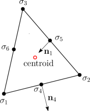
Figure 1: normals for (5). Left: $P_{2}$-element; Right: $P_{3}$-element.

$$\dfrac{{\rm d}\mathbf{u}_{\sigma}}{{\rm d}t}+\sum\limits_{E,\sigma\in E}\Phi_{\sigma}^{E}(\mathbf{u})=0,$$ (5a)

with

$$\Phi_{\sigma}^{E}(\mathbf{u})=N_{\sigma}\big{(}K_{\sigma}^{E})^{+}\mathbf{J}(\mathbf{u}_{\sigma})\cdot\nabla\mathbf{u}(\sigma),$$ (5b)

where $${\mathbf{n}}_{\sigma} \sigma$$ is sum of the inward normals of the sides that contain (see figure 1),

$$K_{\sigma}^{E}=\mathbf{J}(\mathbf{u}_{\sigma})\cdot{\mathbf{n}}_{\sigma}^{E}\text{ and }N_{\sigma}^{-1}=\sum\limits_{E,\sigma\in E}\big{(}K_{\sigma}^{E}\big{)}^{+}.$$ (5c)

so that consistency is obvious. From [9], one can see that the matrix $N$ exists. A slightly different version is

$$\Phi_{\sigma}^{E}(\mathbf{u})=N_{\sigma}\text{ sign}\big{(}K_{\sigma}^{E})\mathbf{J}(\mathbf{u}_{\sigma})\cdot\nabla\mathbf{u},\qquad N_{\sigma}^{-1}=\sum\limits_{E,\sigma\in E}\text{sign}\big{(}K_{\sigma}^{E}\big{)}.$$

3.2 Low order schemes

For the average value, one can simply take a standard finite volume (so we do not use the boundary values). We have taken the Lax-Friedrichs numerical flux and the Roe scheme in our simulations.

The real problem is what to do with the point values. A first order version

             

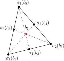
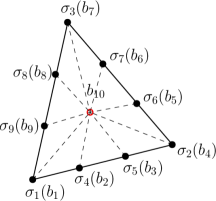
Figure 2: Geometry for the first order scheme. Left: $P_{2}$-element; Right: $P_{3}$-element.

can be defined as follows. We first, and temporarily for the definition of sub-elements only, re-number the boundary nodes. We pick one degree of freedom, call it $b_{1}$, and list the other in a counter-clockwise manner: we get the list $\{b_{1},\ldots,b_{N-1}\}$ of all the boundary degrees of freedom. The centroid is denoted by $b_{N}$, with $N=7$ for a quadratic approximation, and $N=10$ for the cubic one. Then we define the sub-elements of vertices $\{b_{i},b_{N},b_{i+1}\}$ with a numbering modulo $N$. This defines $N-1$ sub-elements that we denote by $T^{E}_{i}$, then we get inwards normals ${\mathbf{n}}_{b_{i}}^{l}$. For quadratic elements, and using back the original numbering, this is illustrated in Figure 2. In what follows, we use the original numbering with this geometrical definition of sub-elements.

The update of $\mathbf{u}_{\sigma}$ is done with (5) where $\Phi_{\sigma}^{E}$ needs to be modified. We use

$$\Phi_{\sigma}^{E}=\frac{1}{|C_{\sigma}|}\sum_{T^{E}_{i},\sigma\in T^{E}_{i}}\Phi_{\sigma}^{T^{E}_{i}}(\mathbf{u}).$$ (6)

The residuals will be defined the following, which is done to get monotone first order residual distribution schemes, see [8, 10] for example. We will use two types of residuals:

• a version that is inspired by the Local Lax-Friedrichs scheme

  $$\Phi_{\sigma}^{T^{E}_{i}}=\frac{1}{3}\oint_{T^{E}_{i}}\mathbf{J}(\mathbf{u})\cdot\nabla\mathbf{u}\;{\rm d}\mathbf{x}+\alpha_{T^{E}_{i}}\big{(}\mathbf{u}_{\sigma}-\overline{\mathbf{u}}_{T^{E}_{i}}\big{)}$$

  with

  $$\oint_{T^{E}_{i}}\mathbf{J}(\mathbf{u})\cdot\nabla\mathbf{u}\;{\rm d}\mathbf{x}\approx|T^{E}_{i}|\mathbf{J}(\overline{\mathbf{u}}_{T^{E}_{i}})\nabla\mathbf{u}({\color[rgb]{0,0,0}\hbox{\vbox{\hrule height=0.5pt\kern 1.72218pt\hbox{\kern-0.50003pt$\mathbf{u}$\kern 0.0pt}}}_{T^{E}_{i}}}),$$ (7)

  where we use the $\mathbb{P}^{1}$ approximation on $T^{E}_{i}$ and $\overline{\mathbf{u}}_{T^{E}_{i}}$ is the arithmetic average of the $\mathbf{u}$’s at three vertices of $T^{E}_{i}$ (hence we use the average value here). Last,

  $$\alpha_{T^{E}_{i}}\geq\max\limits_{\begin{subarray}{c}{\color[rgb]{0,0,0}\sigma\in T^{E}_{i},}\\ {\mathbf{n}}_{b}^{i}\text{ normals of }T^{E}_{i}\end{subarray}}\rho\big{(}\mathbf{J}({\color[rgb]{0,0,0}\mathbf{u}_{\sigma}})\cdot{\mathbf{n}}_{b}^{i}\big{)},$$

  where $\rho(B)$ is the spectral radius of the matrix $B$.

• A version that is inspired by the finite volume scheme rewritten in the residual distribution framework, see [11] for details. We have used the Roe scheme with Harten-Yee entropy fix.

We still need to define $|C_{\sigma}|$. It is

$$|C_{\sigma}|=\sum_{E,\sigma\in E}\sum_{T^{E}_{i},\sigma\in T^{E}_{i}}\frac{|T^{E}_{i}|}{3},$$

and after some simple calculations, we see that

$$|C_{\sigma}|=\sum_{E,\sigma\in E}\frac{2|E|}{3{\color[rgb]{0,0,0}(N-1)}}.$$

The low order version can easily be shown to be invariant domain preserving under some CFL conditions. For example, the Local Lax-Friedrichs version needs that

$$3\frac{\Delta t}{|T^{E}_{i}|}\rho\big{(}\mathbf{J}(\mathbf{u}_{\sigma})\cdot{\mathbf{n}}_{b}^{i}\big{)}\leq 1,\qquad\forall E,i$$

and this condition turns out to be much more restrictive than the one we can use in practice.

3.3 Linear stability

Linear stability is not easy to study when the mesh has no particular symmetry, and when the scheme under consideration does not satisfy a variational principle. In the one dimensional case, it was possible to show that the scheme developed in [6] is linearly stable: this has been done by W. Barsukow and reported in [7] using [12]. However, the scheme (5), adapted in 1D, would not be exactly the same as in [6]. So we have conducted an experimental study on several types of meshes generated by GMSH [13] with several types of meshing option (frontal Delaunay, Delaunay). The all proved to be stable for the linear and non-linear problems tested above, with a CFL halved with respect to the standard value for quadratic approximation and divided by 3 for the cubic approximation. This is more or less what is expected because for quadratic (resp. cubic) approximation, the density of degrees of freedom is approximately doubled (resp. tripled).

For the first order approximation, using Rusanov, it is easy to get a CFL condition for which the solution stays in its domain of dependence.

3.4 Non linear stabilisation

When the solution develops discontinuities, the high order scheme will be prone to numerical oscillations. To overcome this, we have used a simplified version of the MOOD paradigm, [14, 15]. Since point values and average are independent variables, we need to test both.

The idea is to work with several schemes ranging from order $p=3\text{ or }4$ to $1$, with the lowest order one able to provide results staying in the invariance domain. For the element $E$, we write the scheme for $\hbox{\vbox{\hrule height=0.5pt\kern 1.72218pt\hbox{\kern-0.50003pt$\mathbf{u}$\kern 0.0pt}}}_{E}$ as $S_{E}(k)$ and for $u_{\sigma}$ as $S_{\sigma}(k)$.

We denote by $\mathbf{u}^{n}_{E}$ and $\mathbf{u}_{\sigma}^{n}$ the solution at the time $t_{n}$. After each Runge-Kutta cycle, the updated solution is denoted by $\tilde{\mathbf{u}}_{E}$, $\tilde{\mathbf{u}}_{\sigma}$.

We first run the full order scheme, for each Runge-Kutta cycle. Concerning the average $\mathbf{u}_{E}$, we store the flux $\int_{\Gamma}{\mathbf{f}}(\mathbf{u}^{h})\cdot{\mathbf{n}}$ for reasons of conservation. Then, for the average,

1. Computer Admissible Detector (CAD in short): We check if $\tilde{\mathbf{u}}_{E}$ is a valid vector with real components: we check if each component is not NaN. Else, we flag the element and go to the next one in the list,

2. Physically Admissible Detector (PAD in short):We check if $\tilde{\mathbf{u}}_{E}\in\mathcal{D}$. If this is false, the element is flagged, and go to the next one in the list.

3. Then we check if at $t_{n}$, the solution is not constant in the elements used in the numerical stencil (so we check and compare between the average and point values $u_{\sigma}$ in $E$ with those in the elements sharing a face with $E$). This is done in order to avoid to detect a fake maximum principle. If the solution is declared locally constant, we move to the next element.

4. Discrete Maximum Principle (DMP in short): we check if $\tilde{\mathbf{u}}_{E}$ is a local extrema. if we are dealing with the Euler equations, we compute the density and the pressure and perform this test on these two values only, even though for a system this is not really meaningful. We denote by $\xi$ the functional on which we perform the test (i.e. $\mathbf{u}_{F}$ itself for scalar problems, and the density/pressure obtained from $V(E)$, the set of elements elements $F$ that share a face or a vertex with $E$, excluding $E$ itself. We say we have a potential extrema if

   $$\xi_{E}^{n+1}\not\in[\big{(}\min\limits_{F\in V(E)}\xi_{F}^{n}\big{)}{\color[rgb]{0,0,0}-}\varepsilon_{E}^{n},\big{(}\max\limits_{F\in V(E)}\xi_{F}^{n}\big{)}{\color[rgb]{0,0,0}+}\varepsilon_{E}^{n}],$$

   where $\varepsilon_{E}^{n}$ estimated as in [14]. If the test is wrong, we go to the next element, else the element is flagged.

If an element is flagged, then each of its faces are flagged, and recompute the flux of the flagged faces using the first order scheme.

For the point values, the procedure is similar, and then for the flagged degrees of freedom, we recompute

$$\sum\limits_{E,\sigma\in E}\Phi_{\sigma}^{E}(\mathbf{u}^{n})$$

with the first order scheme.

4 Numerical results

In this section, we demonstrate the performance of the developed schemes in §3 on several numerical examples. When MOOD is activated, we use the local Rusanov scheme (with a small stencil) as described in §3.2. The CFL number (based on the elements) is always set to $0.4$.

4.1 Scalar case

We begin with the scalar case,

$$\dfrac{\partial u}{\partial t}+\mathbf{a}(\mathbf{x})\cdot\nabla u=0,$$ (8)

with, for $\mathbf{x}=(x,y)$, $\mathbf{a}(\mathbf{x})=\big{(}a^{(1)},a^{(2)}\big{)}$ representing the velocity field that the quantity $u$ is moving with.

4.1.1 Convection problem

In the first example, we consider $\mathbf{a}(\mathbf{x})=2\pi\big{(}-(y-y_{0}),x-x_{0}\big{)}$ and note that $\text{ div }\mathbf{a}=0$, so that (8) can be put in a conservation form. The domain is $\Omega=[-20,20]^{2}$, $(x_{0},y_{0})=(0,0)$ and the initial condition is

$$u_{0}(\mathbf{x})=e^{-\|\mathbf{x}-\mathbf{\tilde{x}}_{0}\|^{2}},~{}~{}\mathbf{\tilde{x}}_{0}=(5,5).$$ (9)

The solution is checked after one rotation ($T=1$) with the exact one. The initial mesh is obtained with GMSH, using the front Delaunay option. Then we subdivide the mesh by cutting the edges into two equal or three equal segments, and a quadratic approximation or a cubic approximation is employed. The discrete $L^{1}$-, $L^{2}$-, and $L^{\infty}$-errors of the point values $u$ computed with quadratic and cubic approximations are shown on Tables 1 and 2, respectively. As one can clearly see that, the expected third- and fourth-order accuracy is achieved.

Table 1: Errors and rates for the initial condition (9) with the quadratic approximation of (2)-(5).

$h$	$L^{1}$	rate	$L^{2}$	rate	$L^{\infty}$	rate
$2.00\times 10^{-1}$	$4.309\times 10^{-1}$	-	$6.703\times 10^{-2}$	-	$3.270\times 10^{-2}$	-
$1.91\times 10^{-1}$	$3.749\times 10^{-1}$	2.85	$5.857\times 10^{-2}$	2.77	$2.871\times 10^{-2}$	2.66
$1.82\times 10^{-1}$	$3.241\times 10^{-1}$	3.13	$5.079\times 10^{-2}$	3.06	$2.512\times 10^{-2}$	2.87
$1.74\times 10^{-1}$	$2.850\times 10^{-1}$	2.89	$4.485\times 10^{-2}$	2.80	$2.215\times 10^{-2}$	2.83
$1.67\times 10^{-1}$	$2.553\times 10^{-1}$	2.59	$4.026\times 10^{-2}$	2.54	$2.007\times 10^{-2}$	2.39
$1.60\times 10^{-1}$	$2.269\times 10^{-1}$	2.89	$3.584\times 10^{-2}$	2.84	$1.786\times 10^{-2}$	2.78
$1.33\times 10^{-1}$	$1.317\times 10^{-1}$	2.98	$2.100\times 10^{-2}$	2.93	$1.056\times 10^{-2}$	2.88

Table 2: Same as in Table 1 but with the cubic approximation.

$h$	$L^{1}$	rate	$L^{2}$	rate	$L^{\infty}$	rate
$4.00\times 10^{-1}$	$5.219\times 10^{-1}$	-	$6.800\times 10^{-2}$	-	$2.206\times 10^{-2}$	-
$3.33\times 10^{-1}$	$2.440\times 10^{-1}$	4.17	$3.268\times 10^{-2}$	4.02	$1.121\times 10^{-2}$	3.71
$2.86\times 10^{-1}$	$1.358\times 10^{-1}$	3.80	$1.839\times 10^{-2}$	3.73	$6.339\times 10^{-3}$	3.70
$2.50\times 10^{-1}$	$7.978\times 10^{-2}$	3.99	$1.083\times 10^{-2}$	3.96	$3.705\times 10^{-3}$	4.02
$2.22\times 10^{-1}$	$4.868\times 10^{-2}$	4.19	$6.634\times 10^{-3}$	4.16	$2.321\times 10^{-3}$	3.97
$2.00\times 10^{-1}$	$3.267\times 10^{-2}$	4.19	$4.458\times 10^{-3}$	4.16	$1.542\times 10^{-3}$	3.97

4.1.2 Zalesak test case

In the second example, we consider a Zalesak’s problem, which involves the solid body rotation of a notched disk. Here the domain is $[0,1]^{2}$ and the rotation field is $\mathbf{a}(\mathbf{x})$ also defined to be a rotation with respect to $(x_{0},y_{0})=(0.5,0.5)$ and angular speed of $2\pi$. The initial condition is

$$u_{0}(\mathbf{x})=\left\{\begin{array}[]{ll}0.25\big{(}1+\cos(\frac{\pi r_{1}}{0.15}))&\text{ if }r_{1}=\|\mathbf{x}-(0.25,0.5)\|\leq 0.15,\\ 1-\frac{r_{2}}{0.15}&\text{ if }r_{2}=\|\mathbf{x}-(0.5,0.25)\|\leq 0.15,\\ 1&\text{ if }r_{3}=\|\mathbf{x}-(0.5,0.75)\|\leq 0.15,\\ 0&\text{ if }|x-0.5|\leq 0.025~{}\text{ and }~{}y\in[0.6,0.85].\end{array}\right.$$

We use the MOOD procedure and compute the numerical solution with a mesh that has 3442 vertices, 10123 edges, and 16881 elements (hence 13565 (resp. 40569) DoFs in total for quadratic (resp. cubic) approximation, thanks to the Euler relation). The results computed by quadratic approximation after 1, 2, and 3 rotations are displayed in Figures 3–4.

(a) point values $\mathbf{u}_{\sigma}$

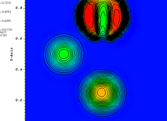
(b) average values $\hbox{\vbox{\hrule height=0.5pt\kern 1.37775pt\hbox{\kern-0.40002pt$\mathbf{u}$\kern 0.0pt}}}_{E}$

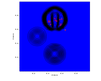
(c) flag on $\mathbf{u}_{\sigma}$

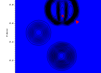
(d) flag on $\hbox{\vbox{\hrule height=0.5pt\kern 1.37775pt\hbox{\kern-0.40002pt$\mathbf{u}$\kern 0.0pt}}}_{E}$

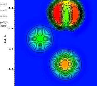
(e) point values $\mathbf{u}_{\sigma}$

(f) average values $\hbox{\vbox{\hrule height=0.5pt\kern 1.37775pt\hbox{\kern-0.40002pt$\mathbf{u}$\kern 0.0pt}}}_{E}$

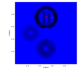
(g) flag on $\mathbf{u}_{\sigma}$

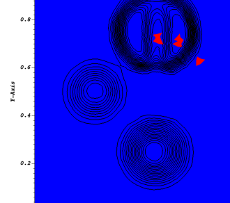
(h) flag on $\hbox{\vbox{\hrule height=0.5pt\kern 1.37775pt\hbox{\kern-0.40002pt$\mathbf{u}$\kern 0.0pt}}}_{E}$

(i) point values $\mathbf{u}_{\sigma}$

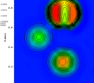
(j) average values $\hbox{\vbox{\hrule height=0.5pt\kern 1.37775pt\hbox{\kern-0.40002pt$\mathbf{u}$\kern 0.0pt}}}_{E}$

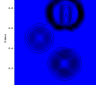
(k) flag on $\mathbf{u}_{\sigma}$

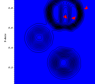
(l) flag on $\hbox{\vbox{\hrule height=0.5pt\kern 1.37775pt\hbox{\kern-0.40002pt$\mathbf{u}$\kern 0.0pt}}}_{E}$

Figure 3: Zalesak problem: quadratic approximation and MOOD criteria are checked expect for PAD. Top row: $T=1$; Middle row: $T=2$; Bottom row: $T=3$.

From the subplots in the first two columns of these figures, one can observe that, both the point values and the average values can be correctly captured. In the last two columns of these figures, we also indicate in red where the MOOD criteria are violated. We first check the criteria expect for PAD. From the subplots in the last two columns of Figure 3, we see that, as expected, the first order scheme is only used around the region where the solution is non-smooth. We also observe that the minimum value of $\mathbf{u}_{\sigma}$ and $\hbox{\vbox{\hrule height=0.5pt\kern 1.72218pt\hbox{\kern-0.50003pt$\mathbf{u}$\kern 0.0pt}}}_{E}$ is $\approx-10^{-2}$. This is due to the fact that the PAD is not checked.

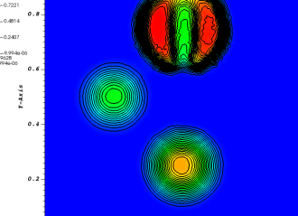
(a) point values $\mathbf{u}_{\sigma}$

(b) average values $\hbox{\vbox{\hrule height=0.5pt\kern 1.37775pt\hbox{\kern-0.40002pt$\mathbf{u}$\kern 0.0pt}}}_{E}$

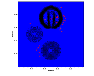
(c) flag on $\mathbf{u}_{\sigma}$

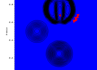
(d) flag on $\hbox{\vbox{\hrule height=0.5pt\kern 1.37775pt\hbox{\kern-0.40002pt$\mathbf{u}$\kern 0.0pt}}}_{E}$

(e) point values $\mathbf{u}_{\sigma}$

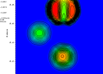
(f) average values $\hbox{\vbox{\hrule height=0.5pt\kern 1.37775pt\hbox{\kern-0.40002pt$\mathbf{u}$\kern 0.0pt}}}_{E}$

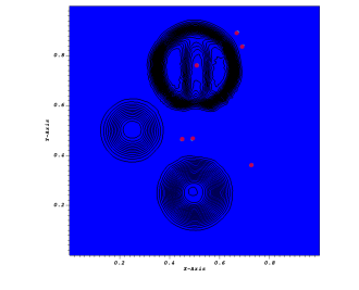
(g) flag on $\mathbf{u}_{\sigma}$

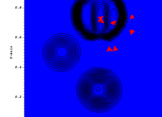
(h) flag on $\hbox{\vbox{\hrule height=0.5pt\kern 1.37775pt\hbox{\kern-0.40002pt$\mathbf{u}$\kern 0.0pt}}}_{E}$

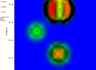
(i) point values $\mathbf{u}_{\sigma}$

(j) average values $\hbox{\vbox{\hrule height=0.5pt\kern 1.37775pt\hbox{\kern-0.40002pt$\mathbf{u}$\kern 0.0pt}}}_{E}$

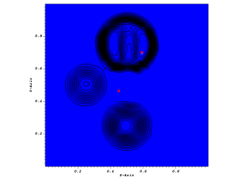
(k) flag on $\mathbf{u}_{\sigma}$

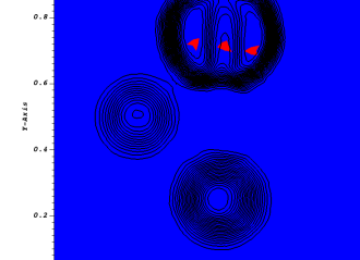
(l) flag on $\hbox{\vbox{\hrule height=0.5pt\kern 1.37775pt\hbox{\kern-0.40002pt$\mathbf{u}$\kern 0.0pt}}}_{E}$

Figure 4: Same as in Figure 3 but all MOOD criteria are checked.

We then check all the MOOD criteria including PAD, and say that PAD is violated if $\mathbf{u}_{\sigma}<-10^{-5}$ or $\hbox{\vbox{\hrule height=0.5pt\kern 1.72218pt\hbox{\kern-0.50003pt$\mathbf{u}$\kern 0.0pt}}}_{E}<-10^{-5}$. From the subplots in the last two columns of Figure 4, we clearly see that the first-order scheme will be also used in the region where the solution is smooth but PAD may not be satisfied. At the same time, we can see that the minimum value of $\mathbf{u}_{\sigma}$ and $\hbox{\vbox{\hrule height=0.5pt\kern 1.72218pt\hbox{\kern-0.50003pt$\mathbf{u}$\kern 0.0pt}}}_{E}$ is $>-10^{-5}$, which satisfies the assumed PAD criterion.

Finally, we compute the solution using cubic approximation. For saving space, only the results obtained with checking all MOOD criteria are presented in Figure 5. Comparing the sensor results with those computed by quadratic approximation, we observe that cubic approximation leads to less activation of MOOD paradigm.

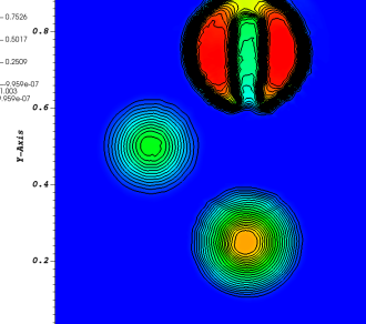
(a) point values $\mathbf{u}_{\sigma}$

(b) average values $\hbox{\vbox{\hrule height=0.5pt\kern 1.37775pt\hbox{\kern-0.40002pt$\mathbf{u}$\kern 0.0pt}}}_{E}$

(c) flag on $\mathbf{u}_{\sigma}$

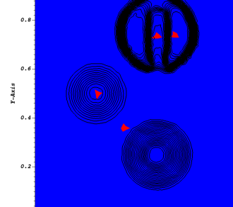
(d) flag on $\hbox{\vbox{\hrule height=0.5pt\kern 1.37775pt\hbox{\kern-0.40002pt$\mathbf{u}$\kern 0.0pt}}}_{E}$

(e) point values $\mathbf{u}_{\sigma}$

(f) average values $\hbox{\vbox{\hrule height=0.5pt\kern 1.37775pt\hbox{\kern-0.40002pt$\mathbf{u}$\kern 0.0pt}}}_{E}$

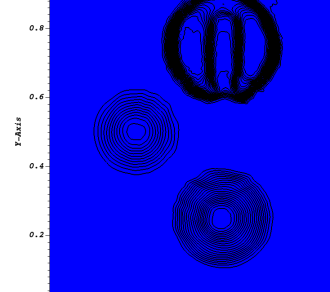
(g) flag on $\mathbf{u}_{\sigma}$

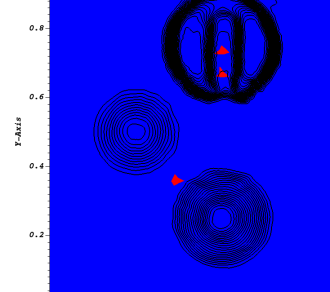
(h) flag on $\hbox{\vbox{\hrule height=0.5pt\kern 1.37775pt\hbox{\kern-0.40002pt$\mathbf{u}$\kern 0.0pt}}}_{E}$

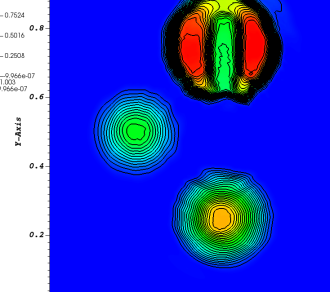
(i) point values $\mathbf{u}_{\sigma}$

(j) average values $\hbox{\vbox{\hrule height=0.5pt\kern 1.37775pt\hbox{\kern-0.40002pt$\mathbf{u}$\kern 0.0pt}}}_{E}$

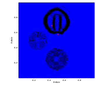
(k) flag on $\mathbf{u}_{\sigma}$

(l) flag on $\hbox{\vbox{\hrule height=0.5pt\kern 1.37775pt\hbox{\kern-0.40002pt$\mathbf{u}$\kern 0.0pt}}}_{E}$

Figure 5: Same as in Figure 4 but using cubic approximation.

4.1.3 KPP test case

In the third example, we consider the KPP problem which has been first considered by Kurganov, Popov and Petrova in [16]. The governing PDE is

$$\dfrac{\partial u}{\partial t}+\dfrac{\partial\big{(}{\color[rgb]{0,0,0}\sin}\;u\big{)}}{\partial x}+\dfrac{\partial\big{(}{\color[rgb]{0,0,0}\cos}\;u\big{)}}{\partial y}=0,$$ (10)

in a domain $[-2,2]^{2}$ with the initial condition

$$u_{0}(\mathbf{x})=\left\{\begin{array}[]{ll}\frac{7}{2}\pi&\text{ if }\|\mathbf{x}-(0,0.5)\|^{2}\leq 1,\\ \frac{\pi}{4}&\text{ else.}\end{array}\right.$$

The problem (10) is non-convex, in the sense that compound wave may exist. Here we have used the MOOD paradigm with the Local Lax-Friedrichs scheme as a first order scheme. We compute the numerical solution until final time $T=1$ using both the quadratic and cubic approximations. For the $P_{2}$ (resp. $P_{3}$) elements, the mesh has 8601 vertices, 25480 edges, 16880 elements, and 34081 (resp. 76441) degrees of freedom. We present the obtained numerical results in Figures 6 and 7.

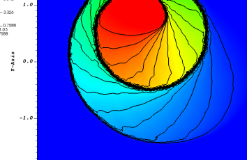
(a) point values $\mathbf{u}_{\sigma}$

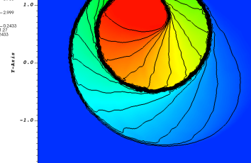
(b) average values $\hbox{\vbox{\hrule height=0.5pt\kern 1.37775pt\hbox{\kern-0.40002pt$\mathbf{u}$\kern 0.0pt}}}_{E}$

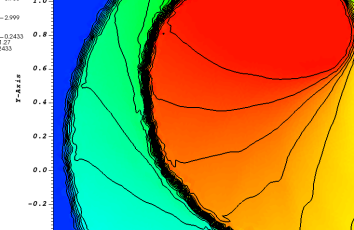
(c) zoom of average values

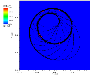
(d) flag on point values $\mathbf{u}_{\sigma}$

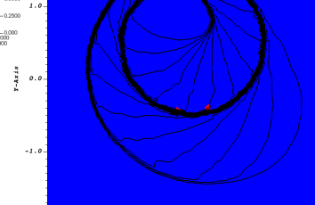
(e) flag on average values $\hbox{\vbox{\hrule height=0.5pt\kern 1.37775pt\hbox{\kern-0.40002pt$\mathbf{u}$\kern 0.0pt}}}_{E}$

Figure 6: KPP problem: using quadratic approximation.

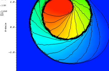
(a) point values $\mathbf{u}_{\sigma}$

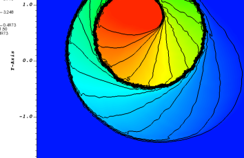
(b) average values $\hbox{\vbox{\hrule height=0.5pt\kern 1.37775pt\hbox{\kern-0.40002pt$\mathbf{u}$\kern 0.0pt}}}_{E}$

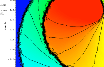
(c) zoom of average values

(d) flag on point values $\mathbf{u}_{\sigma}$

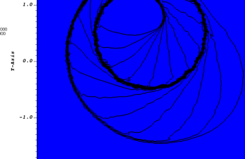
(e) flag on average values $\hbox{\vbox{\hrule height=0.5pt\kern 1.37775pt\hbox{\kern-0.40002pt$\mathbf{u}$\kern 0.0pt}}}_{E}$

Figure 7: Same as in Figure 6 but using cubic approximation.

Same as in Figure 6 but

If the method is not dissipative enough, the two shocks in the northwest direction at around $22^{\circ}$ will be attached and this is not correct. Here this is not the case, and the solution looks correct, at least in comparison with the existing literature on the subject. We are not aware of any form of exact analytical solution. We also indicate in red where the computed quantities ($\mathbf{u}_{\sigma}$ or $\hbox{\vbox{\hrule height=0.5pt\kern 1.72218pt\hbox{\kern-0.50003pt$\mathbf{u}$\kern 0.0pt}}}_{E}$) violate MOOD criteria (PAD is included) given in §3.4. As one can see, the low-order scheme is only activated at a limited number of locations. When the cubic approximation is used, the average values does not violate the MOOD criteria at the final time.

4.2 Euler equations

We proceed with Euler equations of gas dynamics and consider the following six cases:

• A stationary vortex case in $[-10,10]^{2}$ for $T=3$.

• A moving vortex case in $[-20,20]^{2}$ for $T=20$.

• The Sod problem in $[-1,1]^{2}$ for $T=0.16$.

• The 13th case studied by Liu and Lax [17], where the solution is shown at time $T=1$.

• The 3rd case of [18] by Kurganov and Tadmor. Here $T=1$.

• The double Mach reflection case of Woodward and Collela, [19].

4.2.1 Accuracy test

In the first example of nonlinear system case, we verify the order of convergence of the proposed schemes. To this end, we consider a smooth stationary isentropic vortex flow. The computational domain is $[-10,10]\times[-10,10]$ with Dirichelet boundary conditions everywhere. The initial condition is given by

$$\rho=(1+\delta T)^{\frac{1}{\gamma-1}},\quad u=-\frac{\varepsilon}{2\pi}x_{2}e^{\frac{1-r^{2}}{2}},\quad v=\frac{\varepsilon}{2\pi}x_{1}e^{\frac{1-r^{2}}{2}},\quad p=\rho^{\gamma},$$ (11)

where the vortex strength is $\varepsilon=5$ and $\delta T=-\frac{(\gamma-1)\varepsilon^{2}}{8\gamma\pi^{2}}e^{1-r^{2}}$ with $r=\|\mathbf{x}\|=\sqrt{x_{1}^{2}+x_{2}^{2}}$. This is a stationary equilibrium of the system so the exact solution coincides with the initial condition at any time. The proposed scheme is not able to exactly preserve this equilibrium state and the truncation error is $\mathcal{O}(h^{p})$, where $h$ is the characteristic size of the triangular mesh and $p$ is the order of the scheme. Thus, it severs as a good numerical example to verify the order of convergence; see also, e.g. in [20, 21].

Tables 3– 6 report the convergence rates of $P_{2}$ and $P_{3}$ approximations for the vortex test problem run on a sequence of successively refined meshes. The meshes are obtained from the Cartesian $40\times 40$, $80\times 80$, $160\times 160$, $320\times 320$, and $640\times 640$ meshes which are all cut by the diagonal. From the obtained results, we can clearly see that the expected third- and fourth-accuracy is achieved by the proposed schemes with quadratic and cubic approximations, respectively.

Table 3: Errors and rates on the average values of density, quadratic approximation, $T=3$.

$h$	$L^{1}$	rate	$L^{2}$	rate	$L^{\infty}$	rate
$3.6262\times{10^{-1}}$	$1.262\times 10^{-4}$	-	$2.850\times 10^{-5}$	-	$8.406\times 10^{-3}$	-
$1.7901\times{10^{-1}}$	$2.220\times 10^{-5}$	$2.46$	$4.851\times 10^{-6}$	$2.51$	$1.364\times 10^{-3}$	$2.58$
$8.8944\times{10^{-2}}$	$3.179\times 10^{-6}$	$2.78$	$6.865\times 10^{-7}$	$2.80$	$2.058\times 10^{-4}$	$2.70$
$4.4332\times{10^{-2}}$	$4.172\times 10^{-7}$	$2.92$	$9.093\times 10^{-8}$	$2.90$	$2.843\times 10^{-5}$	$2.84$
$2.2132\times{10^{-2}}$	$5.298\times 10^{-8}$	$2.97$	$1.160\times 10^{-8}$	$2.96$	$3.660\times 10^{-6}$	$2.95$

Table 4: Same as in Table 3 but for point values of density

$h$	$L^{1}$	rate	$L^{2}$	rate	$L^{\infty}$	rate
$2.9608\times{10^{-1}}$	$9.100\times 10^{-5}$	-	$2.696\times 10^{-5}$	-	$1.979\times 10^{-2}$	-
$1.4616\times{10^{-1}}$	$1.526\times 10^{-5}$	$2.53$	$4.083\times 10^{-6}$	$2.68$	$1.960\times 10^{-3}$	$3.28$
$7.2623\times{10^{-2}}$	$2.182\times 10^{-6}$	$2.78$	$5.799\times 10^{-7}$	$2.79$	$2.355\times 10^{-4}$	$3.03$
$3.6198\times{10^{-2}}$	$2.860\times 10^{-7}$	$2.92$	$7.685\times 10^{-8}$	$2.90$	$3.323\times 10^{-5}$	$2.81$
$1.8070\times{10^{-2}}$	$3.630\times 10^{-8}$	$2.97$	$9.796\times 10^{-9}$	$2.96$	$4.356\times 10^{-6}$	$2.92$

Table 5: Errors and rates on the average values of density, cubic approximation, $T=3$.

$h$	$L^{1}$	rate	$L^{2}$	rate	$L^{\infty}$	rate
$3.6262\times{10^{-1}}$	$1.956\times 10^{-5}$	-	$4.651\times 10^{-6}$	-	$2.051\times 10^{-3}$	-
$1.7901\times{10^{-1}}$	$8.975\times 10^{-7}$	$4.37$	$1.603\times 10^{-7}$	$4.77$	$5.134\times 10^{-5}$	$5.22$
$8.8944\times{10^{-2}}$	$4.970\times 10^{-8}$	$4.14$	$8.579\times 10^{-9}$	$4.19$	$3.373\times 10^{-6}$	$3.89$
$4.4332\times{10^{-2}}$	$1.867\times 10^{-7}$	$4.08$	$4.829\times 10^{-10}$	$4.13$	$2.895\times 10^{-9}$	$4.16$
$2.2132\times{10^{-2}}$	$1.755\times 10^{-10}$	$4.03$	$2.863\times 10^{-11}$	$4.07$	$1.128\times 10^{-8}$	$4.04$

Table 6: Same as in Table 5 but for point values of density.

$h$	$L^{1}$	rate	$L^{2}$	rate	$L^{\infty}$	rate
$2.4175\times{10^{-1}}$	$1.462\times 10^{-5}$	-	$4.990\times 10^{-6}$	-	$2.169\times 10^{-3}$	-
$1.1934\times{10^{-1}}$	$6.647\times 10^{-7}$	$4.38$	$1.713\times 10^{-7}$	$4.78$	$9.512\times 10^{-5}$	$4.43$
$5.9296\times{10^{-2}}$	$3.733\times 10^{-8}$	$4.12$	$9.757\times 10^{-9}$	$4.10$	$5.200\times 10^{-6}$	$4.16$
$2.9555\times{10^{-2}}$	$2.253\times 10^{-9}$	$4.03$	$5.953\times 10^{-10}$	$4.02$	$3.018\times 10^{-7}$	$4.09$
$1.4754\times{10^{-2}}$	$1.399\times 10^{-10}$	$4.00$	$3.798\times 10^{-11}$	$3.96$	$2.254\times 10^{-8}$	$3.73$

4.2.2 Moving vortex problem

In the second example of nonlinear system case, we consider the following initial condition:

$$\rho=\big{(}T_{\infty}+\Delta T\big{)}^{\frac{1}{\gamma-1}},\quad u=u_{\infty}-{y_{2}}Me^{\frac{1-R}{2}},\quad v=v_{\infty}+y_{1}Me^{\frac{1-R}{2}},\quad p=\rho^{\gamma},$$ (12)

prescribed in the domain $[-20,20]^{2}$. In (12), $(u_{\infty},v_{\infty})=(1,\frac{\sqrt{2}}{2})$, $T_{\infty}=1$, $M=\frac{5}{2\pi}$, $\mathbf{y}=({\bf x-x_{0}})/2$ with $\mathbf{x}_{0}=(-10,-10)$, $R=\|\mathbf{y}\|^{2}$, and $\Delta T=-\frac{\gamma-1}{2\gamma}M^{2}e^{{1-R}}$. This vortex is simply advected with the velocity $(u_{\infty},v_{\infty})$ so that it is very easy to compute the exact solution. The third- and fourth-order results at final time $T=20$, for the scheme (2)-(5), are shown in Figures 8 and 9. The mesh as well as a comparison with the exact solution is also shown. We have also displayed zooms of the solution at $T=20$, superimposed with the exact one. For the fourth order case, it is difficult to see a difference, at this scale, between the exact and numerical solutions. In the two cases, the mesh that is plotted is obtained from the actual computational mesh where we have subdivided the elements using the Lagrange points: these meshes represent all the degrees of freedom that we actually use. It turns out that the plotting meshes (represented) are identical for the two types of solutions.

(a) $P_{2}$-element: point values $\rho_{\sigma}$

(b) $P_{2}$-element: zoom of $\rho_{\sigma}$

(c) $P_{2}$-element: average values $\hbox{\vbox{\hrule height=0.5pt\kern 1.37775pt\hbox{\kern-0.40002pt$\rho$\kern 0.0pt}}}_{E}$

(d) $P_{2}$-element: zoom of $\hbox{\vbox{\hrule height=0.5pt\kern 1.37775pt\hbox{\kern-0.40002pt$\rho$\kern 0.0pt}}}_{E}$

Figure 8: Moving vortex problem: $\rho$, zoom of the solution and the mesh. The exact solution is in black lines, the numerical solution with colored isolines. The mesh has 69705 DoFs, 35082 elements, third order scheme.

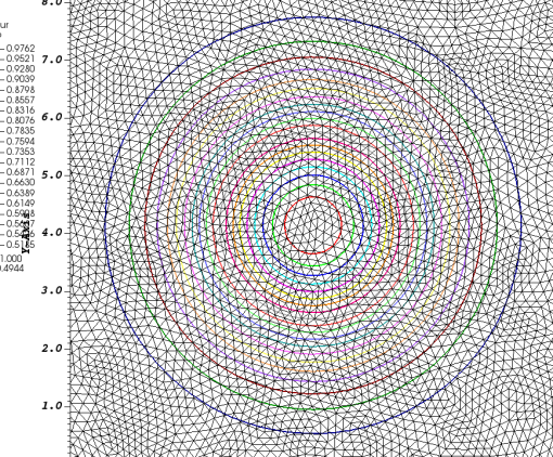
(a) $P_{3}$-element: point values $\rho_{\sigma}$

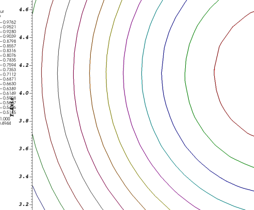
(b) $P_{3}$-element: zoom of $\rho_{\sigma}$

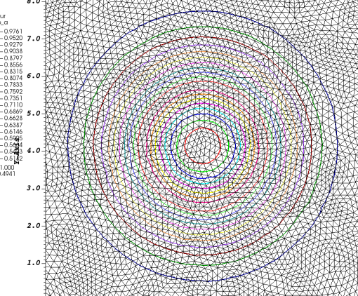
(c) $P_{3}$-element: average values $\hbox{\vbox{\hrule height=0.5pt\kern 1.37775pt\hbox{\kern-0.40002pt$\rho$\kern 0.0pt}}}_{E}$

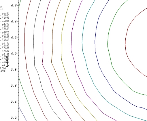
(d) $P_{3}$-element: zoom of $\hbox{\vbox{\hrule height=0.5pt\kern 1.37775pt\hbox{\kern-0.40002pt$\rho$\kern 0.0pt}}}_{E}$

Figure 9: Moving vortex problem: $\rho$, zoom of the solution and the mesh. The exact solution is in black lines, the numerical solution with colored isolines. The mesh has 70762 DoFs, 15930 elements, fourth order scheme.

4.2.3 2D Sod problem

In the third example of nonlinear system case, we test the proposed schemes on a well-known 2D Sod benchmark problem. The initial condition is given by

$$(\rho,u,v,p)=\left\{\begin{aligned} &(1,0,0,1.5)&&\mbox{if}~{}\|\mathbf{x}\|^{2}\leq 0.25,\\ &(0.125,0,0,0.1)&&\mbox{else},\end{aligned}\right.$$

the boundary condition is solid wall, and the final time we compute is $T=0.16$. The two approximations (quadratic and cubic) have been used to compute the solution. We plot the results (density component) in Figure 10. As one can see, both two approximations produce similar results and cubic approximation is much more accurate as expected. In Figure 11, we also plot the flags where the first-order scheme is activated at the final time. We can clearly see that only the first-order scheme for the point values is used and the cubic approximation leads to less triggers of the first-order scheme.

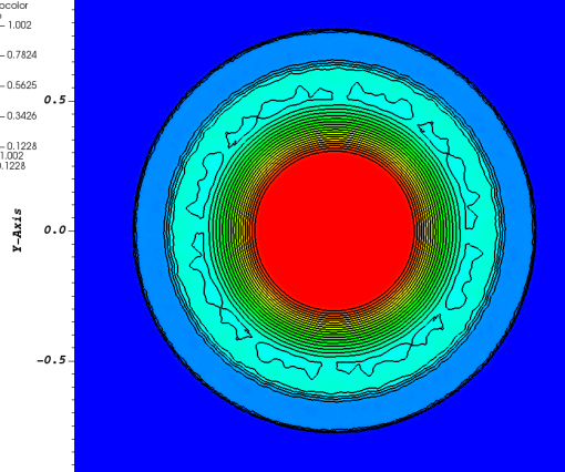
(a) point values $\rho_{\sigma}$ using $P_{2}$-element

(b) average values $\hbox{\vbox{\hrule height=0.5pt\kern 1.37775pt\hbox{\kern-0.40002pt$\rho$\kern 0.0pt}}}_{E}$ using $P_{2}$-element

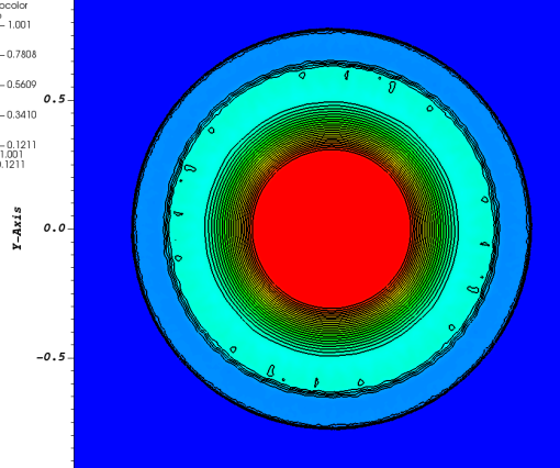
(c) point values $\rho_{\sigma}$ using $P_{3}$-element

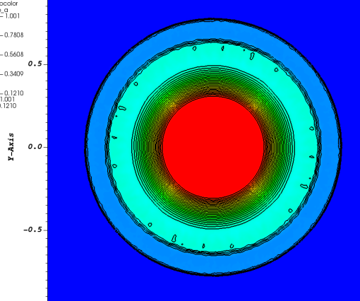
(d) average values $\hbox{\vbox{\hrule height=0.5pt\kern 1.37775pt\hbox{\kern-0.40002pt$\rho$\kern 0.0pt}}}_{E}$ using $P_{3}$-element

Figure 10: Sod problem: profiles of density.

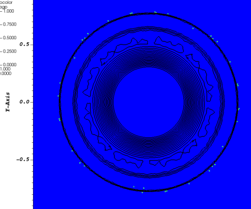
(a) flag on $\rho_{\sigma}$ using $P_{2}$-element

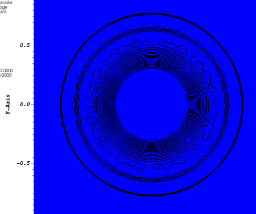
(b) flag on $\hbox{\vbox{\hrule height=0.5pt\kern 1.37775pt\hbox{\kern-0.40002pt$\rho$\kern 0.0pt}}}_{E}$ using $P_{2}$-element

(c) flag on $\rho_{\sigma}$ using $P_{3}$-element

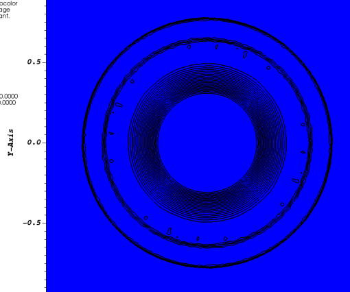
(d) flag on $\hbox{\vbox{\hrule height=0.5pt\kern 1.37775pt\hbox{\kern-0.40002pt$\rho$\kern 0.0pt}}}_{E}$ using $P_{3}$-element

Figure 11: Sod problem: flags at the positions first-order scheme is used.

4.2.4 Liu-Lax problem

In the fourth example of nonlinear system case, we consider the following initial condition

$$(\rho,u,v,p)=\left\{\begin{array}[]{ll}(\rho_{1},u_{1},v_{1},p_{1})=(0.5313,0,0,0.4)&\text{ if }x\geq 0\text{ and }y\geq 0,\\ (\rho_{2},u_{2},v_{2},p_{2})=(1,0.7276,0,1)&\text{ if }x\leq 0\text{ and }y\geq 0,\\ (\rho_{3},u_{3},v_{3},p_{3})=(0.8,0,0,1)&\text{ if }x\leq 0\text{ and }y\leq 0,\\ (\rho_{4},u_{4},v_{4},p_{4})=(1,0,0.7276,1)&\text{ if }x\geq 0\text{ and }y\leq 0,\end{array}\right.$$

prescribed in the computational domain $[-2,2]^{2}$. The states 1 and 2 are separated by a shock. The states 2 and 3 are separated by slip line. The states 3 and 4 are separated by a steady slip-line. The states 4 and 1 are separated by a shock. The mesh has $53227$ vertices, $158878$ edges, $105652$ elements, and $212105$ (resp. $476635$) DoFs for quadratic (resp. cubic) approximation. The obtained results of density field are plotted in Figure 12.

(a) point values $\rho_{\sigma}$ using $P_{2}$-element

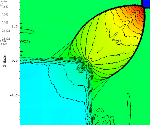
(b) average values $\hbox{\vbox{\hrule height=0.5pt\kern 1.37775pt\hbox{\kern-0.40002pt$\rho$\kern 0.0pt}}}_{E}$ using $P_{2}$-element

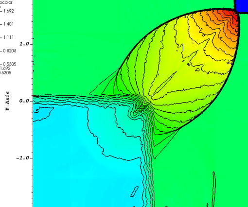
(c) point values $\rho_{\sigma}$ using $P_{3}$-element

(d) average values $\hbox{\vbox{\hrule height=0.5pt\kern 1.37775pt\hbox{\kern-0.40002pt$\rho$\kern 0.0pt}}}_{E}$ using $P_{3}$-element

Figure 12: Liu-Lax case: profiles of density.

4.2.5 Kurganov-Tadmor problem

In the fifth example of nonlinear system case, the initial condition is

$$(\rho,u,v,p)=\left\{\begin{array}[]{ll}(\rho_{1},u_{1},v_{1},p_{1})=(1.5,0,0,1.5)&\text{ if }x\geq 1\text{ and }y\geq 1,\\ (\rho_{2},u_{2},v_{2},p_{2})=(0.5323,1.206,0,0.3)&\text{ if }x\leq 1\text{ and }y\geq 1,\\ (\rho_{3},u_{3},v_{3},p_{3})=(0.138,1.206,1.206,0.029)&\text{ if }x\leq 1\text{ and }y\leq 1,\\ (\rho_{4},u_{4},v_{4},p_{4})=(0.5323,0,1.206,0.3)&\text{ if }x\leq 1\text{ and }y\leq 1.\end{array}\right.$$

Here the four states are separated by shocks. The domain is $[0,1.2]^{2}$. The solution at $T=1$ is displayed in Figure 13. The mesh has $53140$ vertices, $158617$ edges, $105478$ elements, and $211757$ (resp. $475852$) DoFs for quadratic (resp. cubic) approximation. We see that, on one hand, the solution looks very similar to what is obtained in the literature; see e.g. in [22, 23, 24]. On the other hand, the first order schemes (for average and point values) are activated on very few positions, see Figure 14.

(a) point values $\rho_{\sigma}$ using $P_{2}$-element

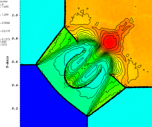
(b) average values $\hbox{\vbox{\hrule height=0.5pt\kern 1.37775pt\hbox{\kern-0.40002pt$\rho$\kern 0.0pt}}}_{E}$ using $P_{2}$-element

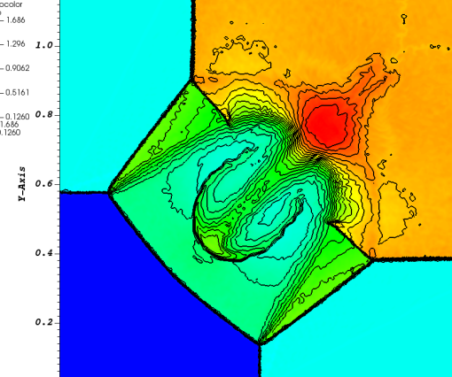
(c) point values $\rho_{\sigma}$ using $P_{3}$-element

(d) average values $\hbox{\vbox{\hrule height=0.5pt\kern 1.37775pt\hbox{\kern-0.40002pt$\rho$\kern 0.0pt}}}_{E}$ using $P_{3}$-element

Figure 13: Kurganov-Tadmor problem: profiles of density.

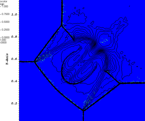
(a) flag on $\rho_{\sigma}$ using $P_{2}$-element

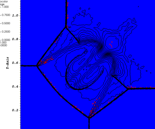
(b) flag on $\hbox{\vbox{\hrule height=0.5pt\kern 1.37775pt\hbox{\kern-0.40002pt$\rho$\kern 0.0pt}}}_{E}$ using $P_{2}$-element

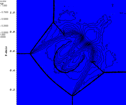
(c) flag on $\rho_{\sigma}$ using $P_{3}$-element

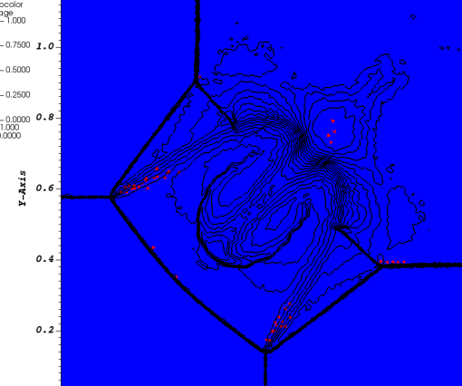
(d) flag on $\hbox{\vbox{\hrule height=0.5pt\kern 1.37775pt\hbox{\kern-0.40002pt$\rho$\kern 0.0pt}}}_{E}$ using $P_{3}$-element

Figure 14: Kurganov-Tadmor problem: flags at the positions first-order scheme is used.

4.2.6 Woodward-Collela problem

In the final example of nonlinear system case, we consider a double Mack reflection problem. The domain is a ramp, and initially a shock at Mach 10 is set at $x=0$. The mesh has $29290$ vertices, $57870$ elements and $87159$ edges, i.e. $116449$ (reps. $261478$) DoFs for $P_{2}$ (reps. $P_{3}$) approximations. The right condition is

$$(\rho_{R},u_{R},v_{R},p_{R})=(\gamma,0,0,1)$$

so that the speed of sound is $1$ ($\gamma=1.4$) and the left state is obtained assuming a shock at Mach 10, so that

$$(\rho_{L},u_{L},v_{L},p_{L})=(8,8.25,0,116.5).$$

The solution at $T=0.2$ is shown on Figure 15. We observe slight oscillations in the numerical solution, indicating the need for carefully designing limiting strategies or adjusting the MOOD criteria. This will be the focus of our future research. We also display the location where the first order scheme is activated at the final time; see Figure 16.

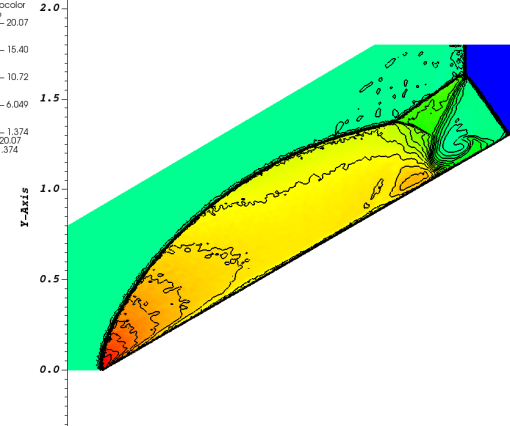
(a) point values $\rho_{\sigma}$ using $P_{2}$-element

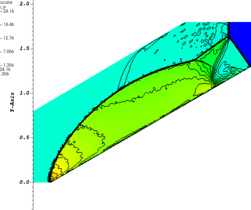
(b) average values $\hbox{\vbox{\hrule height=0.5pt\kern 1.37775pt\hbox{\kern-0.40002pt$\rho$\kern 0.0pt}}}_{E}$ using $P_{2}$-element

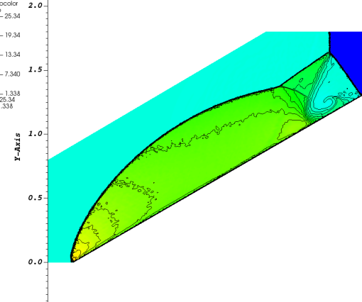
(c) point values $\rho_{\sigma}$ using $P_{3}$-element

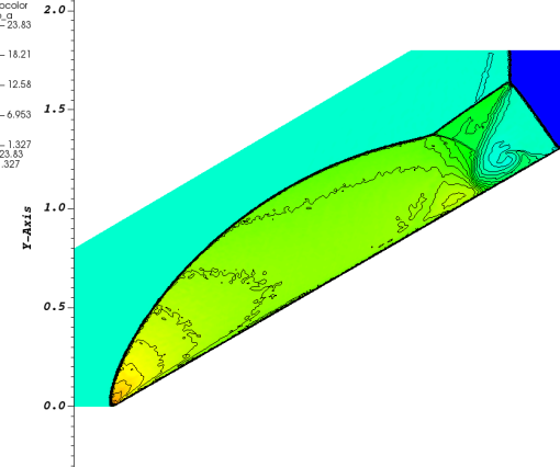
(d) average values $\hbox{\vbox{\hrule height=0.5pt\kern 1.37775pt\hbox{\kern-0.40002pt$\rho$\kern 0.0pt}}}_{E}$ using $P_{3}$-element

Figure 15: Woodward-Collela problem: profiles of density.

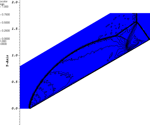
(a) flag on $\rho_{\sigma}$ using $P_{2}$-element

(b) flag on $\hbox{\vbox{\hrule height=0.5pt\kern 1.37775pt\hbox{\kern-0.40002pt$\rho$\kern 0.0pt}}}_{E}$ using $P_{2}$-element

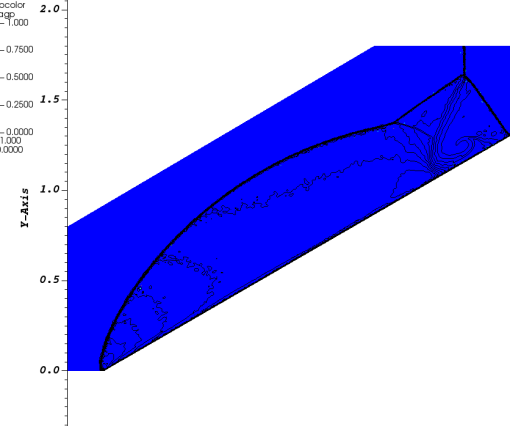
(c) flag on $\rho_{\sigma}$ using $P_{3}$-element

(d) flag on $\hbox{\vbox{\hrule height=0.5pt\kern 1.37775pt\hbox{\kern-0.40002pt$\rho$\kern 0.0pt}}}_{E}$ using $P_{3}$-element

Figure 16: Woodward-Collela problem: flags at the positions first-order scheme is used.

5 Conclusions

We have presented a computational method inspired by the so-called Active flux method, following the ideas developed in [6] and [7], and using triangular type meshes. The method is able to handle shocks. We have illustrated the behavior of this method on several cases with smooth and discontinuous problems and models ranging from scalar to systems. The behavior of the method is as expected.

Appendix A Boundary conditions for the Euler case.

We have considered two type of boundary condition on $\partial\Omega$ where $\Omega\subset\mathbb{R}^{2}$: wall boundary conditions and inflow/outflow. We describe how they are implemented for the update of the averages and the point values.

A.1 Average values

Inside the domain, $\hbox{\vbox{\hrule height=0.5pt\kern 1.72218pt\hbox{\kern-0.50003pt$\mathbf{u}$\kern 0.0pt}}}_{E}$ will satisfy:

$$|E|\dfrac{{\rm d}{\color[rgb]{0,0,0}\hbox{\vbox{\hrule height=0.5pt\kern 1.72218pt\hbox{\kern-0.50003pt$\mathbf{u}$\kern 0.0pt}}}_{E}}}{{\rm d}t}+\oint_{\partial E}\hat{\mathbf{f}}_{\mathbf{n}}(\mathbf{u}^{h},\mathbf{u}^{-})\;{\color[rgb]{0,0,0}{\rm d}\gamma}={\color[rgb]{0,0,0}|E|\dfrac{{\rm d}\hbox{\vbox{\hrule height=0.5pt\kern 1.72218pt\hbox{\kern-0.50003pt$\mathbf{u}$\kern 0.0pt}}}_{E}}{{\rm d}t}+}\sum_{\Gamma\text{edge of }E}\int_{\Gamma}\hat{\mathbf{f}}_{\mathbf{n}}(\mathbf{u}^{h},\mathbf{u}^{-})\;{\color[rgb]{0,0,0}{\rm d}\Gamma}{\color[rgb]{0,0,0}=0},$$

where the numerical flux is the continuous one for the high order scheme and a standard numerical flux for the first order case. Here, $\mathbf{u}^{h}$ is the value of $\mathbf{u}$ on the boundary of $\partial E$, $\mathbf{u}^{-}$ is the value on the opposite side of the element, and ${\mathbf{n}}$ is the local normal.

If one edge $\Gamma$ is contained in $\partial\Omega$, we modify

$$\int_{\Gamma}\hat{\mathbf{f}}_{\mathbf{n}}(\mathbf{u}^{h},\mathbf{u}^{-})\;{\rm d}\gamma\approx|\Gamma|\sum_{\text{ quadrature points }}\omega_{q}\hat{\mathbf{f}}_{\mathbf{n}}(\mathbf{u}^{h}(\mathbf{x}_{q}),\mathbf{u}^{-}(\mathbf{x}_{q}))$$

evaluated by quadrature. We use a Gaussian quadrature with 3 points.

• for wall, by setting the state $\mathbf{u}^{-}(\mathbf{x}_{q})$ equal to the state obtained from $\mathbf{u}^{h}(\mathbf{x}_{q})$ by symmetry with respect to $\Gamma$, i.e. same density, same pressure, but the velocity $\mathbf{v}$ is

  $$\mathbf{v}^{-}(\mathbf{x}_{q})=\mathbf{v}^{h}(\mathbf{x}_{q})-2\frac{\langle\mathbf{v}^{h}(\mathbf{x}_{q}),{\mathbf{n}}\rangle}{\|{\mathbf{n}}\|^{2}}{\mathbf{n}}.$$

• for inflow/outflow, since we want to impose $\mathbf{u}=\mathbf{u}_{\infty}$ weakly, we take $\mathbf{u}^{-}=\mathbf{u}^{\infty}$, and the flux is some upwind flux (the Roe one for the numerical experiments).

• For supersonic inflow/outflows or if the solution stays constant in a neighborhood of the boundary, we will impose Neumann Conditions, i.e. we force the solution to stay constant.

A.2 Point values

It is a bit more involved. Let us remind that the update of the solution is made by (5a),

$$\dfrac{{\rm d}\mathbf{u}_{\sigma}}{{\rm d}t}+\sum\limits_{E,\sigma\in E}\Phi_{\sigma}^{E}(\mathbf{u})=0$$

that we have to modify into

$$\dfrac{{\rm d}\mathbf{u}_{\sigma}}{{\rm d}t}+\sum\limits_{E,\sigma\in E}\Phi_{\sigma}^{E}(\mathbf{u})+\sum_{\Gamma\subset\partial{\color[rgb]{0,0,0}\Omega},\sigma\in\Gamma}\Phi_{\sigma}^{\Gamma}(\mathbf{u})=0$$ (13)

and we need to define $\Phi_{\sigma}^{\Gamma}(\mathbf{u})$. We do it in two cases: wall and Neumann conditions.

• Neumann condition: again, we force the solution to stay the same, i.e.

  $$\sum\limits_{E,\sigma\in E}\Phi_{\sigma}^{E}(\mathbf{u})+\sum_{\Gamma\subset\partial{\color[rgb]{0,0,0}\Omega},\sigma\in\Gamma}\Phi_{\sigma}^{\Gamma}(\mathbf{u})=0.$$

  In practice, once $\sum\limits_{E,\sigma\in E}\Phi_{\sigma}^{E}(\mathbf{u})$ has been computed, we set this quantity to $0$.

• Wall. For each $\Gamma$ in (13), with normal ${\mathbf{n}}$, there is one element $E$ that has $\Gamma$ as one of its edges. Then we consider $E^{-}$, the (virtual) element that is symmetric with respect to ${\mathbf{n}}$. We consider $\mathbf{u}^{-}$, the state symmetric to $\mathbf{u}^{h}$ with respect to ${\mathbf{n}}$, i.e. same density and pressure, symmetric velocity. Using this we define $\Phi^{\Gamma}(\mathbf{u}^{h})$ by $\Phi^{\Gamma}(\mathbf{u}^{h})=\Phi^{E^{-}}(\mathbf{u}^{-})$.

References

• [1] T.A. Eyman and P.L. Roe. Active flux. 49th AIAA Aerospace Science Meeting, 2011.
• [2] T.A. Eyman and P.L. Roe. Active flux for systems. 20 th AIAA Computationa Fluid Dynamics Conference, 2011.
• [3] T.A. Eyman. Active flux. PhD thesis, University of Michigan, 2013.
• [4] C.ย Helzel, D.ย Kerkmann, and L.ย Scandurra. A new ADER method inspired by the active flux method. Journal of Scientific Computing, 80(3):35โ€“61, 2019.
• [5] W.ย Barsukow. The active flux scheme for nonlinear problems. J. Sci. Comput., 86(1):Paper No. 3, 34, 2021.
• [6] R.ย Abgrall. A combination of residual distribution and the active flux formulations or a new class of schemes that can combine several writings of the same hyperbolic problem: application to the 1d Euler equations. Commun. Appl. Math. Comput., 5(1):370โ€“402, 2023.
• [7] Remi Abgrall and Wasilij Barsukow. Extensions of active flux to arbitrary order of accuracy. ESAIM, Math. Model. Numer. Anal., 57(2):991โ€“1027, 2023.
• [8] H.ย Deconinck and M.ย Ricchiuto. Encyclopedia of Computational Mechanics, chapter Residual distribution schemes: foundation and analysis. John Wiley & sons, 2007. DOI: 10.1002/0470091355.ecm054.
• [9] R.ย Abgrall. Toward the ultimate conservative scheme: Following the quest. J. Comput. Phys., 167(2):277โ€“315, 2001.
• [10] R.ย Abgrall. Essentially non oscillatory residual distribution schemes for hyperbolic problems. J. Comput. Phys, 214(2):773โ€“808, 2006.
• [11] R.ย Abgrall. Some remarks about conservation for residual distribution schemes. Comput. Methods Appl. Math., 18(3):327โ€“351, 2018.
• [12] John J.ย H. Miller. On the location of zeros of certain classes of polynomials with applications to numerical analysis. J. Inst. Math. Appl., 8:397โ€“406, 1971.
• [13] Christophe Geuzaine and Jean-Franรงois Remacle. Gmsh: a 3-D finite element mesh generator with built-in pre- and post-processing facilities. Int. J. Numer. Methods Eng., 79(11):1309โ€“1331, 2009.
• [14] S.ย Clain, S.ย Diot, and R.ย Loubรจre. A high-order finite volume method for systems of conservation lawsโ€”Multi-dimensional Optimal Order Detection (MOOD). J. Comput. Phys., 230(10):4028โ€“4050, 2011.
• [15] F.ย Vilar. A posteriori correction of high-order discontinuous Galerkin scheme through subcell finite volume formulation and flux reconstruction. J. Comput. Phys., 387:245โ€“279, 2019.
• [16] Alexander Kurganov, Guergana Petrova, and Bojan Popov. Adaptive semidiscrete central-upwind schemes for nonconvex hyperbolic conservation laws. SIAM J. Sci. Comput., 29(6):2381โ€“2401, 2007.
• [17] Xu-Dong Liu and Peterย D. Lax. Solution of two-dimensional riemann problems of gas dynamics by positive schemes. SIAM J. Sci. Comput., 19:319โ€“340, 1998.
• [18] Alexander Kurganov and Eitan Tadmor. Solution of two-dimensional Riemann problems for gas dynamics without Riemann problem solvers. Numer. Methods Partial Differ. Equations, 18(5):584โ€“608, 2002.
• [19] P.ย Woodward and P.ย Colella. The numerical solution of two-dimensional fluid flow with strong shocks. Journal of Computational Physics, 54:115โ€“173, 1988.
• [20] E.ย Gaburro, W.ย Boscheri, S.ย Chiocchetti, C.ย Klingenberg, V.ย Springel, and M.ย Dumbser. High order direct Arbitrary-Lagrangian-Eulerian schemes on moving Voronoi meshes with topology changes. Journal of Computational Physics, 407:109167, 2020.
• [21] R.ย Abgrall, P.ย Bacigaluppi, and S.ย Tokareva. High-order residual distribution scheme for the time-dependent Euler equations of fluid dynamics. Computers and Mathematics with Applications, 78:274โ€“297, 2019.
• [22] A.ย Kurganov, Y.ย Liu, and V.ย Zeitlin. Numerical dissipation switch for two-dimensional central-upwind schemes. ESAIM Mathematical Modelling and Numerical Analysis, 55:713โ€“734, 2021.
• [23] N.ย K. Grag, A.ย Kurganov, and Y.ย Liu. Semi-discrete central-upwind Rankine-Hugoniot schemes for hyperbolic systems of conservation laws. Journal of Computational Physics, 428:110078, 2021.
• [24] B.-S. Wang, W.ย Don, A.ย Kurganov, and Y.ย Liu. Fifth-order A-WENO schemes based on the adaptive diffusion central-upwind Rankine-Hugoniot fluxes. Communications on Applied Mathematics and Computation, 5:295โ€“314, 2023.