An invariant measure of chiral quantum transport

Abstract:

We study the invariant measure of the transport correlator for a chiral Hamiltonian and analyze its properties. The Jacobian of the invariant measure is a function of random phases. Then we distinguish the invariant measure before and after the phase integration. In the former case we found quantum diffusion of fermions and a uniform zero mode that is associated with particle conservation. After the phase integration the transport correlator reveals two types of evolution processes, namely classical diffusion and back-folded random walks. Which one dominates the other depends on the details of the underlying chiral Hamiltonian and may lead either to classical diffusion or to the suppression of diffusion.

1 Introduction

We consider the quantum evolution of a particle from the site ${\bf r}^{\prime}$ to the site ${\bf r}$ during the time period $t$ in a particle conserving system. Then the building block for quantum transport is provided by the transition probability $|\langle{\bf r}|e^{-iHt}|{\bf r}^{\prime}\rangle|^{2}$, which is obtained from the transition amplitude $\langle{\bf r}|e^{-iHt}|{\bf r}^{\prime}\rangle$ over time $t$ for a system defined by the Hamiltonian $H$. We can Laplace transform the amplitude with respect to time and calculate the resulting transition probability, the transport correlator, as

$$\Big{|}\int_{0}^{\infty}\langle{\bf r}|e^{-iHt}|{\bf r}^{\prime}\rangle e^{-\epsilon t}dt\Big{|}^{2}=|G_{{\bf r}{\bf r}^{\prime}}(\epsilon)|^{2},$$ (1)

where $G(\epsilon)=(H-i\epsilon)^{-1}$ is the one-particle Green’s function. Besides the spatial coordinates ${\bf r}$, the Hamiltonian can also depend on additional quantum numbers, such as a spinor or band index. Quantum transport in multiband systems has been a popular subject in recent years due to the discovery of new materials, beginning with graphene [1], topological insulators [2, 3, 4] and including more specialized models such as two-dimensional models with random gauge field [5].

To describe realistic transport in a disordered material we must include random scattering. This can be attributed to a random Hamiltonian $H$. A very successful approach to random scattering is based on the random matrix theory [6, 7], where $H$ is a symmetric or Hermitian matrix with independently and identically distributed matrix elements $H_{ij}$ for $i\leq j$. Many interesting properties (e.g., level repulsion statistics) can be calculated from the invariant measure. This is based on the idea that the fluctuations of the $N$ eigenvalues of, for instance, a symmetric $N\times N$ random matrix $H$, which are invariant under the orthogonal transformation of the matrix, are separated from the remaining $N(N-1)/2$ random degrees of freedom of the matrix elements. Then the Jacobian of the latter provides the invariant measure. This concept can also been applied to the more general class of random matrices, which are defined on a lattice and describe hopping of quantum particles on this lattice [8]. Instead of fixing the eigenvalues of these matrices, one can also use a uniform approximation of the matrix that is fixed by a variational approach (saddle-point approximation). Then the fluctuations induced by the chiral symmetry are represented as the invariant measure.

The goal of the following analysis is to start from the disorder averaged transport correlator $\langle|G_{{\bf r}{\bf r}^{\prime}}(\epsilon)|^{2}\rangle_{d}$ and reduce the general disorder average $\langle\ldots\rangle_{d}$ by the integration with respect to its invariant measure. The justification of this reduction is that the long-range behavior is associated with the invariant measure of the underlying chiral property of a particle-hole symmetric Hamiltonian $H$. It will be shown that the invariant measure provides the long-range properties even before performing the phase integration.

The paper is organized as follows. After a brief discussion of the chiral Hamiltonian $H$, the related Green’s functions, and the corresponding chiral invariance in Sect. 2, we give a summary of the invariant measure, which was originally derived in a previous paper, in Sect. 3. This is followed by an analysis of the corresponding Jacobian and a discussion of the effects caused by phase averaging. In Sect. 4 the different mappings, related to the derivation of the invariant measure, are summarized and an example for a simple two-band Hamiltonian is studied. Finally, we provide some conclusions with open problems and a brief outlook in Sect. 5.

2 Model

The transport correlator in Eq. (1) is a fundamental quantity for the description of quantum transport [9], consisting of products of matrix elements of the advanced and the retarded one-particle Green’s function $G(\pm\epsilon)=(H\pm i\epsilon)^{-1}$ in the form of $G_{{\bf r}{\bf r}^{\prime}}(\epsilon)G_{{\bf r}^{\prime}{\bf r}}(-\epsilon)=(H-i\epsilon)^{-1}_{{\bf r}{\bf r}^{\prime}}(H+i\epsilon)^{-1}_{{\bf r}^{\prime}{\bf r}}$. In the following we consider a multiband Hamiltonian $H$ on a $d$-dimensional lattice $\Lambda$ with $|\Lambda|<\infty$ sites and assume that it is related to its transposed $H^{T}$ through the chiral relation $UH^{T}U^{\dagger}=-H$, where $U$ is a spatially uniform unitary matrix. Then the chiral relation implies that the trace and the determinant for the advanced/retarded Green’s functions obey ${\rm Tr}[G(-\epsilon)]=-{\rm Tr}[G(\epsilon)]$ and $\det[G(-\epsilon)]=\det[-G(\epsilon)]$. Using the Pauli matrices $\{\sigma_{j}\}_{j=1,2,3}$ and the $2\times 2$ unit matrix $\sigma_{0}$, a two-band Hamiltonian can be expressed by an expansion in terms of these matrices. An example is the Hamiltonian $H=h_{1}\sigma_{1}+h_{2}\sigma_{2}+m\sigma_{3}$ with a random $m$ that is independently and identically distributed on the lattice, while the matrices $h_{1,2}$ act on the lattice. For symmetric matrices $h_{1,2}$ this Hamiltonian satisfies the chiral relation for $U=\sigma_{2}$.

The pair of the advanced and retarded Green’s functions can also be written as blocks of an advanced Green’s function when we replace the Hamiltonian $H$ by the block-diagonal Hamiltonian ${\hat{H}}=diag(H,H^{T})$. Then the corresponding advanced Green’s function reads ${\hat{G}}(\epsilon)=({\hat{H}}-i\epsilon)^{-1}$ and we get $G(\epsilon)={\hat{G}}_{11}(\epsilon)$ and $G(-\epsilon)=-U{\hat{G}}_{22}(\epsilon)U^{\dagger}$. For

$${\hat{S}}=\pmatrix{0&sU\cr s^{\prime}U^{\dagger}&0\cr}$$ (2)

with two independent parameters $s$ and $s^{\prime}$ we obtain for ${\hat{H}}$ the symmetry relation

$$e^{\hat{S}}{\hat{H}}e^{\hat{S}}={\hat{H}},$$ (3)

since ${\hat{H}}$ and ${\hat{S}}$ anticommute. It was shown that this symmetry is associated with an invariant measure [8].

3 Invariant measure

In general, for a random chiral Hamiltonian there exists an invariant measure of the disorder average. To demonstrate this we consider the example of the previous section $H=h_{1}\sigma_{1}+h_{2}\sigma_{2}+m\sigma_{3}$ and assume a random $m_{\bf r}$ at each lattice site ${\bf r}$ that obeys a Gaussian distribution $\exp(-m_{\bf r}^{2}/g)dm_{\bf r}$. To control the strong fluctuations of $|G_{{\bf R}{\bf R}^{\prime}}(\epsilon)|^{2}$ near the poles of the Green’s functions, we transform the random field $m_{\bf r}$ to another random field $Q_{\bf r}$ such that this mapping provides the relation

$$\langle|G_{{\bf R}{\bf R}^{\prime}}(\epsilon)|^{2}\rangle_{d}=\langle Q_{\bf R}Q_{{\bf R}^{\prime}}\rangle_{Q}.$$ (4)

Thus, the average transport correlator is a correlation function of the random field $Q_{\bf r}$ [10]. The mapping $m_{\bf r}\to Q_{\bf r}$ yields a Jacobian, and the Gaussian weight $\exp(-m_{\bf r}^{2}/g)$ transforms to the corresponding weight $P(\{Q_{\bf r}\})$ for the field $Q_{\bf r}$, where the latter is correlated on the lattice. Separating the integration over $Q_{\bf r}$ in two parts, namely one that leaves $P(\{Q_{\bf r}\})$ invariant and one that does not. The former, together with the corresponding Jacobian $J$, defines an invariant measure. More specific, it was shown that for a chiral Hamiltonian the invariant measure is given by an integration over random phases, where the Jacobian is $J=\det C$ with the $|\Lambda|\times|\Lambda|$ random-phase matrix $C$. The elements of this matrix are [8]

$$C_{{\bf r}{\bf r}^{\prime}}=2\delta_{{\bf r}{\bf r}^{\prime}}-\sum_{\mu,\mu^{\prime}=1,2}z_{{\bf r}\mu}h_{{\bf r}\mu,{\bf r}^{\prime}\mu^{\prime}}\sum_{{\bf r}^{\prime\prime}}\sum_{\mu^{\prime\prime}=1,2}h^{\dagger}_{{\bf r}^{\prime}\mu^{\prime},{\bf r}^{\prime\prime}\mu^{\prime\prime}}z^{*}_{{\bf r}^{\prime\prime}\mu^{\prime\prime}}\ {\rm with}\ z_{{\bf r}\mu}=e^{i\alpha_{{\bf r}\mu}}\ (0\leq\alpha_{{\bf r}\mu}<2\pi)$$ (5)

with the non-random $2|\Lambda|\times 2|\Lambda|$ matrix

$$h={\bf 1}+2i\eta(\bar{H}-i\eta-i\epsilon)^{-1},$$ (6)

which represents an effective Green’s function. $\eta$ ($0<\eta<\infty$) is an effective scattering rate, usually obtained either from experimental observations, from numerical simulations or from a self-consistent Born approximation of the average one-particle Green’s function. It is proportional to the average density of states, indicating that on average there are state with non-zero density for $\eta>0$. For our approach it must be positive but its actual value is not important for the subsequent discussion. Finally, ${\bar{H}}$ is the average Hamiltonian: ${\bar{H}}=\langle H\rangle_{d}$. It is crucial to note that in the limit $\epsilon\to 0$ the matrix $h$ is unitary (i.e., $hh^{\dagger}={\bf 1}$). $\epsilon>0$ is only necessary to avoid the uniform zero mode with $\sum_{{\bf r}^{\prime}}C_{{\bf r}{\bf r}^{\prime}}=0$. After removing it from the spectrum (cf. App. A), we can take the limit $\epsilon\to 0$. The phase integration provides the relation

$$\langle|G_{{\bf R}{\bf R}^{\prime}}(\epsilon)|^{2}\rangle_{d}\sim\frac{\langle adj_{{\bf R}{\bf R}^{\prime}}C\rangle_{\alpha}}{\langle\det C\rangle_{\alpha}},$$ (7)

where the adjugate matrix is $adj_{{\bf R}{\bf R}^{\prime}}C\equiv C^{-1}_{{\bf R}{\bf R}^{\prime}}\det C$, which is obtained from the determinant by differentation as

$$\partial_{W_{{\bf R}^{\prime}{\bf R}}}\det(C+W)|_{W=0}=\sum_{\pi}\delta_{{\bf R}\pi({\bf R}^{\prime})}{\rm sgn}\pi\prod_{{\bf r}\neq{\bf R}^{\prime}}C_{{\bf r}\pi({\bf r})}.$$ (8)

The relation $\sim$ preserves the asymptotic properties on large distances $|{\bf R}-{\bf R}^{\prime}|$. The phase average $\langle\ldots\rangle_{\alpha}$ is taken with respect to a statistically independent and uniform distribution of the phases $\{\alpha_{{\bf r}\mu}\}$ on the interval $[0,2\pi)$. We will discuss the phase average only in a second step but treat the invariant measure in the following for a general realization of the random phases. Averaging can be performed explicitly and leads to a loop expansion of the determinant and the adjugate matrix [8].

The random-phase matrix $C$ has some remarkable properties, which will be analyzed subsequently, revealing eventually a spatial scaling behavior of $\langle|G_{{\bf R}{\bf R}^{\prime}}(\epsilon)|^{2}\rangle_{d}$ and quantum diffusion of fermions. To this end we consider the random unitary matrix $u=zhz^{*}$ and rewrite $C$ as

$$C_{{\bf r}{\bf r}^{\prime}}={\rm Tr}_{2}[{\hat{C}}_{{\bf r}{\bf r}^{\prime}}E_{2}]\ \ \ {\rm with}\ \ {\hat{C}}_{{\bf r}\mu,{\bf r}^{\prime}\mu^{\prime}}=\delta_{{\bf r}{\bf r}^{\prime}}\delta_{\mu\mu^{\prime}}-u_{{\bf r}\mu,{\bf r}^{\prime}\mu^{\prime}}\sum_{{\bf r}^{\prime\prime},\mu^{\prime\prime}}u^{\dagger}_{{\bf r}^{\prime}\mu^{\prime},{\bf r}^{\prime\prime}\mu^{\prime\prime}},$$ (9)

where $E_{2}=\sigma_{0}+\sigma_{1}$ and ${\rm Tr}_{2}$ is the trace with respect to $2\times 2$ matrices for a Hamiltonian $H$ with two bands. A generalization to a multiband Hamiltonian is straightforward but not considered explicitly. Moreover, with the $2|\Lambda|\times 2|\Lambda|$ matrix $E$, whose elements are 1, we can write $[u^{\dagger}E]_{{\bf r}\mu}=\sum_{{\bf r}^{\prime\prime},\mu^{\prime\prime}}u^{\dagger}_{{\bf r}\mu,{\bf r}^{\prime\prime}\mu^{\prime\prime}}$ and get

$${\hat{C}}={\bf 1}-u[u^{\dagger}E]_{d}={\bf 1}-uu^{\dagger}+u(u^{\dagger}-[u^{\dagger}E]_{d}),$$ (10)

where $[A]_{d}$ is the diagonal part of the general matrix $A$ and ${\bf 1}-uu^{\dagger}=4\epsilon\eta[{\bar{H}}^{2}+(\eta+\epsilon)^{2}]^{-1}$. Now we split $u^{\dagger}$ into its diagonal part $u^{\prime}:=[u^{\dagger}]_{d}$ and its off-diagonal part $v:=u^{\dagger}-u^{\prime}$ and insert this into $u^{\dagger}-[u^{\dagger}E]_{d}$. This gives

$$u^{\prime}+v-[u^{\prime}E]_{d}-[vE]_{d}=v-[vE]_{d},$$ (11)

since $[u^{\prime}E]_{d}=u^{\prime}$. Thus, the diagonal part $u^{\prime}$ drops out and reveals that $z^{*}(v-[vE]_{d})z=h^{\dagger}-[h^{\dagger}]_{d}-[vE]_{d}$ can be understood as a hopping matrix $z^{*}vz$ with an additional random diagonal part $-[vE]_{d}$. In contrast to the conventional disordered tight-binding model [11, 12, 13, 14], the diagonal term also scales with the hopping matrix $v$, since it consists of a sum of hopping terms. In other words, when $v$ changes as $v\to L^{p}v$ under a change of the lattice constant $a\to La$, the entire matrix $v-[vE]_{d}$ scales with $L^{p}$.

We return to $C$ in Eq. (9) and ${\hat{C}}$ in Eq. (10) and write

$$C=\epsilon C^{\prime}+C^{\prime\prime}\ \ {\rm with}\ \ C^{\prime}=4\eta{\rm Tr}_{2}[(z{\bar{H}}^{2}z^{*}+(\eta+\epsilon)^{2})^{-1}E_{2}],\ \ C^{\prime\prime}={\rm Tr}_{2}[u(v-[vE]_{d})E_{2}].$$ (12)

The properties of the determinant and the adjugate matrix of $C$ are linked to the spectral properties of ${\bf 1}-{u^{\dagger}}^{-1}[u^{\dagger}E]_{d}$ in Eq. (10). To analyze this matrix we rewrite it as a quadratic form in $z$:

$$z_{{\bf r}\mu}(\delta_{{\bf r}{\bf r}^{\prime}}\delta_{{\bf r}{\bf r}^{\prime\prime}}\delta_{\mu\mu^{\prime\prime}}-\sum_{\mu^{\prime}}h^{\dagger-1}_{{\bf r}\mu,{\bf r}^{\prime}\mu^{\prime}}h^{\dagger}_{{\bf r}^{\prime}\mu^{\prime},{\bf r}^{\prime\prime}\mu^{\prime\prime}})z^{*}_{{\bf r}^{\prime\prime}\mu^{\prime\prime}}$$

$$=z_{{\bf r}\mu}\sum_{\mu^{\prime}}(\delta_{{\bf r}{\bf r}^{\prime}}\sum_{\bar{{\bf r}}}h^{\dagger-1}_{{\bf r}\mu,\bar{{\bf r}}\mu^{\prime}}h^{\dagger}_{\bar{{\bf r}}\mu^{\prime},{\bf r}^{\prime\prime}\mu^{\prime\prime}}-h^{\dagger-1}_{{\bf r}\mu,{\bf r}^{\prime}\mu^{\prime}}h^{\dagger}_{{\bf r}^{\prime}\mu^{\prime},{\bf r}^{\prime\prime}\mu^{\prime\prime}})z^{*}_{{\bf r}^{\prime\prime}\mu^{\prime\prime}},$$ (13)

which yields

$$C^{\prime\prime}_{{\bf r}{\bf r}^{\prime}}=2\sum_{\bar{{\bf r}}}(\delta_{{\bf r}{\bf r}^{\prime}}-\delta_{\bar{{\bf r}}{\bf r}^{\prime}})K_{{\bf r}\bar{{\bf r}}}=2(\delta_{{\bf r}{\bf r}^{\prime}}\sum_{\bar{{\bf r}}}K_{{\bf r}\bar{{\bf r}}}-K_{{\bf r}{\bf r}^{\prime}}),$$ (14)

where

$$K_{{\bf r}{\bf r}^{\prime}}=\frac{1}{2}\sum_{\mu,\mu^{\prime},\mu^{\prime\prime}}\sum_{{\bf r}^{\prime\prime}}u^{\dagger-1}_{{\bf r}\mu,{\bf r}^{\prime}\mu^{\prime}}u^{\dagger}_{{\bf r}^{\prime}\mu^{\prime},{\bf r}^{\prime\prime}\mu^{\prime\prime}}\ \ {\rm with}\ \ \sum_{\bar{{\bf r}}}K_{{\bf r}\bar{{\bf r}}}=1.$$ (15)

This indicates that $K_{{\bf r}{\bf r}^{\prime}}$ is formally a random transition amplitude for ${\bf r}^{\prime}\to{\bf r}$ with particle conservation due to $\sum_{\bar{{\bf r}}}K_{{\bf r}\bar{{\bf r}}}=1$. Then $C^{\prime\prime}$, defined in Eq. (14), can be understood as a model for quantum diffusion. In contrast to classical diffusion its transition rates are complex numbers rather than probabilities. On the other hand, the average amplitude is a positive number, given by the isotropic mean

$$\langle K_{{\bf r}{\bf r}^{\prime}}\rangle_{\alpha}=\frac{1}{2}\sum_{\mu,\mu^{\prime}}h^{\dagger-1}_{{\bf r}\mu,{\bf r}^{\prime}\mu^{\prime}}h^{\dagger}_{{\bf r}^{\prime}\mu^{\prime},{\bf r}\mu}=\frac{1}{2}\sum_{\mu,\mu^{\prime}}|h_{{\bf r}\mu,{\bf r}^{\prime}\mu^{\prime}}|^{2}$$ (16)

for $h^{\dagger-1}=h$ in the limit $\epsilon\to 0$. This implies

$$\langle C^{\prime\prime}_{{\bf r}{\bf r}^{\prime}}\rangle_{\alpha}=2(\delta_{{\bf r}{\bf r}^{\prime}}-\langle K_{{\bf r}{\bf r}^{\prime}}\rangle_{\alpha})=2(\delta_{{\bf r}{\bf r}^{\prime}}-\sum_{\mu,\mu^{\prime}}|h_{{\bf r}\mu,{\bf r}^{\prime}\mu^{\prime}}|^{2}).$$ (17)

These results can be interpreted as follows. Before phase average the expansion of the determinant $\det C$ or the adjugate matrix $adj_{{\bf R}{\bf R}^{\prime}}C$ provide quantum walks on the lattice in the form of loops, where a site is only visited once. This reflects the fact that the determinant represents fermions, which obey Pauli’s exclusion principle. Thus, the invariant measure describes quantum diffusion of fermions.

After phase average the physics is quite different though, since the average connects lattice sites ${\bf r}$ and ${\bf r}^{\prime}$, visited by the quantum walk, with the transition amplitude $h^{\dagger}_{{\bf r}{\bf r}^{\prime}}$. The latter decays on large distances exponentially, while on short distances it depends strongly on the specific structure of the Hamiltonian ${\bar{H}}$. This is as if we connect the quantum walk between the two lattice sites by an elastic rubber band with an exponential strength for large stretches. In other words, phase averaging is subject to quantum interference effects, which is sensitive to spatial directions and can cause an anisotropic evolution. The average transition amplitude in Eq. (16) is isotropic, since $\langle K_{{\bf r}{\bf r}^{\prime}}\rangle_{\alpha}$ is equal in all lattice directions. Therefore, the length of the rubber band is the same in all directions. The situation is different though for two consecutive steps ${\bf r}\to{\bf r}^{\prime}\to{\bf r}^{\prime\prime}$:

$$\langle K_{{\bf r}{\bf r}^{\prime}}K_{{\bf r}^{\prime}{\bf r}^{\prime\prime}}\rangle_{\alpha}=\langle K_{{\bf r}{\bf r}^{\prime}}\rangle_{\alpha}\langle K_{{\bf r}^{\prime}{\bf r}^{\prime\prime}}\rangle_{\alpha}+\frac{1}{4}\sum_{\mu,\mu^{\prime},\mu^{\prime\prime},\mu^{\prime\prime\prime}}h^{\dagger-1}_{{\bf r}\mu,{\bf r}^{\prime}\mu^{\prime}}h^{\dagger}_{{\bf r}^{\prime}\mu^{\prime},{\bf r}^{\prime}\mu^{\prime\prime\prime}}h^{\dagger-1}_{{\bf r}^{\prime}\mu^{\prime\prime\prime},{\bf r}^{\prime\prime}\mu^{\prime\prime}}h^{\dagger}_{{\bf r}^{\prime\prime}\mu^{\prime\prime},{\bf r}\mu}.$$ (18)

While the first term on the right-hand side is isotropic, the second term depends on the site ${\bf r}^{\prime\prime}$ relative to ${\bf r}$ and ${\bf r}^{\prime}$. This is visualized in Fig. 1c) and calculated for a special example in Sect. 4. While for the first term the length of the rubber band does not change when going from ${\bf r}^{\prime}$ to any of the available ${\bf r}^{\prime\prime}$ with fixed length $|{\bf r}^{\prime\prime}-{\bf r}^{\prime}|$, the rubber band has different lengths for the second term. The latter favors a return of the quantum walk closer to ${\bf r}$ rather than to move away from ${\bf r}$. This picture can be generalized to more steps, connected by rubber bands between pairs of sites along the quantum walk. In general, there is one specific pairing of sites, where the lengths of the rubber bands are not affected for all possible conformations of the random walks, namely when the sites of the quantum walk are connected in each step. This corresponds to the factorization of the phase average

$$\langle K_{{\bf r}{\bf r}_{1}}\rangle_{\alpha}\cdots\langle K_{{\bf r}_{n-1}{\bf r}_{n}}\rangle_{\alpha}\ ,$$

which is visualized in the lower graph of Fig. 1b). It represents a classical random walk with transition probabilities $\langle K_{{\bf r}{\bf r}^{\prime}}\rangle_{\alpha}\geq 0$ and $\sum_{\bar{{\bf r}}}\langle K_{{\bf r}\bar{{\bf r}}}\rangle_{\alpha}=1$. The co-existence of the classical random walk and the folded walks with rubber bands indicates a competition between those walks. To understand this point better we rewrite the right-hand side of Eq. (7) as

$$\frac{\langle adj_{{\bf R}{\bf R}^{\prime}}C\rangle_{\alpha}}{\langle\det C\rangle_{\alpha}}=\frac{adj_{{\bf R}{\bf R}^{\prime}}\langle C\rangle_{\alpha}+\sum_{j}a_{j;{\bf R}{\bf R}^{\prime}}}{\det\langle C\rangle_{\alpha}+\sum_{j}d_{j}},$$ (19)

where the two sums are finite on a finite lattice and are created by a systematic expansion in terms of truncated correlations (linked cluster expansion) as

$$\langle\prod_{\bf r}C_{{\bf r}\pi({\bf r})}\rangle=\prod_{\bf r}\langle C_{{\bf r}\pi({\bf r})}\rangle+\sum_{{\bf r},{\bf r}^{\prime}}\left[\langle C_{{\bf r}\pi({\bf r})}C_{{\bf r}^{\prime}\pi({\bf r}^{\prime})}\rangle_{\alpha}-\langle C_{{\bf r}\pi({\bf r})}\rangle_{\alpha}\langle C_{{\bf r}^{\prime}\pi({\bf r}^{\prime})}\rangle_{\alpha}\right]\prod_{\bar{{\bf r}}\neq{\bf r},{\bf r}^{\prime}}\langle C_{\bar{{\bf r}}\pi(\bar{{\bf r}})}\rangle_{\alpha}+\cdots$$ (20)

for the determinant and the adjugate matrix. Then it depends on the details of the Hamiltonian ${\bar{H}}$ and on the scattering rate $\eta$, which term dominates the others. On an elementary level, we can compare the first and the second term on the right-hand side of Eq. (18), as discussed in Sect. 4. For large distances the classical random walk would be important. On the other hand, for a given number of steps the sum over all realizations of the classical random walk may have a much smaller weight than the sum over all compactly folded walks, which are created by the rubber bands. Thus, we must compare the weights of all walks with a given number of steps and extract those with the highest weight as dominant.

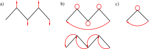
Figure 1: a) A realization of a random walk from site ${\bf r}_{1}$ to site ${\bf r}_{5}$ before phase average, consisting of four steps: $K_{{\bf r}_{1}{\bf r}_{2}}K_{{\bf r}_{2}{\bf r}_{3}}K_{{\bf r}_{3}{\bf r}_{4}}K_{{\bf r}_{4}{\bf r}_{5}}$. According to Eq. (15), the black links represent $u^{\dagger-1}$, while the red arrows represent the factors $\sum_{{\bf r}^{\prime\prime},\mu^{\prime\prime}}u^{\dagger}_{{\bf r}\mu,{\bf r}^{\prime\prime}\mu^{\prime\prime}}$. b) The same random walk after phase average: Two typical contributions are shown for $\langle K_{{\bf r}_{1}{\bf r}_{2}}K_{{\bf r}_{2}{\bf r}_{3}}K_{{\bf r}_{3}{\bf r}_{4}}K_{{\bf r}_{4}{\bf r}_{5}}\rangle_{\alpha}$, where the red connection is $h^{\dagger}$ and corresponds to a “rubber band”. The lower graph represents a classical random walk $\langle K_{{\bf r}_{1}{\bf r}_{2}}\rangle_{\alpha}\langle K_{{\bf r}_{2}{\bf r}_{3}}\rangle_{\alpha}\langle K_{{\bf r}_{3}{\bf r}_{4}}\rangle_{\alpha}\langle K_{{\bf r}_{4}{\bf r}_{5}}\rangle_{\alpha}$. c) This is the two step walk $\langle K_{{\bf r}{\bf r}^{\prime}}K_{{\bf r}^{\prime}{\bf r}^{\prime\prime}}\rangle_{\alpha}-\langle K_{{\bf r}{\bf r}^{\prime}}\rangle_{\alpha}\langle K_{{\bf r}^{\prime}{\bf r}^{\prime\prime}}\rangle_{\alpha}$ of Eq. (18).

4 Discussion of the Results

This work on the invariant measure of the transport properties in chiral systems is based on the random phase matrix $C=\epsilon C^{\prime}+C^{\prime\prime}$ of Eq. (12), whose properties were studied in the previous section. $C$ is connected with the original random Hamiltonian $H$ through several mappings between different random matrices. First, there is the mapping between Hamiltonians

$$H\to z{\bar{H}}z^{*}-i\eta$$ (21)

with the phenomenological scattering rate $\eta>0$. This is accompanied by the mapping of the Green’s function $(H-i\epsilon)^{-1}\to u$ with the effective Green’s function of the Hamiltonian $z{\bar{H}}z^{*}-i\eta$

$$u=zhz^{*}={\bf 1}+2i\eta(z{\bar{H}}z^{*}-i\eta-i\epsilon)^{-1},$$ (22)

from which we eventually get $C$ in Eq. (12) and the transition amplitude $K$ in Eq. (15). $u$ is unitary in the limit $\epsilon\to 0$, which implies the conservative transfer $\sum_{{\bf r}^{\prime}}K_{{\bf r}{\bf r}^{\prime}}=1$ in Eq. (14). The eigenvalues of $u$ are identical with those of $h$ in Eq. (6), which is not random. The corresponding eigenvectors $\Psi_{{\bf k},{\bf r}\mu}$ of $u$ are random though, given by the plane wave $\psi_{{\bf k},{\bf r}}=\exp(i{\bf k}\cdot{\bf r})/\sqrt{|\Lambda|}$ with a random phase factor as $\Psi_{{\bf k},{\bf r}\mu}=z_{{\bf r}\mu}\psi_{{\bf k},{\bf r}}$.

For strong scattering ($\eta\sim\infty$) we get $u\sim-{\bf 1}$, whereas for weak scattering ($\eta\sim 0$) we obtain $u\sim{\bf 1}$. In both limits the transition matrix becomes diagonal with $K={\bf 1}$, implying that the quantum diffusion disappears. All these results are valid before phase averaging. The transport correlator, defined through the relation in Eq. (7), requires phase averaging of $\det C$ and the related adjugate matrix. Although the average can be performed easily, the result leads to complex expressions, which can be associated with classical random walks and folded random walks with rubber bands. On a more elementary level we get for $u$ the diagonal mean $\langle u_{{\bf r}\mu,{\bf r}^{\prime}\mu^{\prime}}\rangle_{\alpha}=\delta_{{\bf r}{\bf r}^{\prime}}\delta_{\mu\mu^{\prime}}h_{{\bf r}\mu,{\bf r}\mu}$ and a vanishing variance, while the mean $\langle C^{\prime\prime}\rangle_{\alpha}$ in Eq. (17) reveals classical diffusion. The fluctuations of $C^{\prime\prime}$ are characterized by the variance

$$\langle{C^{\prime\prime}_{{\bf r}{\bf r}^{\prime}}}^{2}\rangle_{\alpha}-\langle C^{\prime\prime}_{{\bf r}{\bf r}^{\prime}}\rangle_{\alpha}^{2}=\sum_{\mu}\left(\sum_{\mu^{\prime}}|h_{{\bf r}\mu,{\bf r}^{\prime}\mu^{\prime}}|^{2}\right)^{2}.$$ (23)

Then the ratio of the standard deviation and the mean value is

$$R:=\frac{\sqrt{\langle C_{{\bf r}{\bf r}^{\prime}}^{2}\rangle_{\alpha}-\langle C_{{\bf r}{\bf r}^{\prime}}\rangle_{\alpha}^{2}}}{\langle C_{{\bf r}{\bf r}^{\prime}}\rangle_{\alpha}}=\sqrt{1-2p_{1}p_{2}/(p_{1}+p_{2})^{2}}\ \ {\rm with}\ \ p_{\mu}=\sum_{\mu^{\prime}}|h_{{\bf r}\mu,{\bf r}^{\prime}\mu^{\prime}}|^{2},$$ (24)

which is equal or less than 1. In other words, the fluctuations of $C$ around the mean value $\langle C\rangle$ are restricted. Moreover, for $N$ bands with equal $p_{\mu}\equiv{\bar{p}}$ we get $R=N^{-1/2}$, indicating a non-random limit for a large number of bands $N\sim\infty$. In contrast, the fluctuations of $|G_{{\bf r}{\bf r}^{\prime}}(\epsilon)|^{2}$ are unbounded for $\epsilon\sim 0$ due to the proximity to the poles of the Green’s functions. This demonstrates that the invariant measure is better controlled than the original transport correlator.

In order to give an example for the anisotropic effect of the phase averaging, we expand $h$ in powers of $1/\eta$:

$$h=-{\bf 1}+i\frac{1}{\eta}{\bar{H}}+\frac{1}{\eta^{2}}{\bar{H}}^{2}+O(1/\eta^{3}).$$ (25)

Then we choose a band-diagonal matrix ${\bar{H}}=\Delta\sigma_{3}$, where $\Delta$ is nearest-neighbor hopping: $\Delta_{{\bf r}-{\bf r}^{\prime}}=1$ for ${\bf r}$, ${\bf r}^{\prime}$ nearest-neighbor sites and zero otherwise. For the nearest-neighbor vectors ${\bf r}^{\prime}={\bf r}\pm{\bf e}_{1,2}$ on a square lattice with lattice unit vectors ${\bf e}_{1,2}$ we obtain, after neglecting terms of order $1/\eta^{3}$,

$$h_{{\bf r},\mu}=\cases{-1+4/\eta^{2}&${\bf r}=0$\cr(-1)^{\mu}i/\eta&${\bf r}=\pm{\bf e}_{1,2}$\cr 1/\eta^{2}&${\bf r}=\pm({\bf e}_{1}+{\bf e}_{2}),\pm({\bf e}_{1}-{\bf e}_{2}),\pm 2{\bf e}_{1,2}$\cr 0&otherwise\cr}$$ (26)

with $h_{{\bf r}\mu,{\bf r}^{\prime}\mu}\equiv h_{{\bf r}-{\bf r}^{\prime},\mu}$. The weight $|h_{{\bf r}\mu}|$ decreases in powers of $1/\eta$ as we increase the distance $|{\bf r}|$, with the maximal weight $1-4/\eta^{2}$ for ${\bf r}=0$. This yields for the classical diffusion in two steps with the special choice ${\bf r}^{\prime}={\bf r}+{\bf e}_{1}$ and ${\bf r}^{\prime\prime}={\bf r}^{\prime}+{\bf R}={\bf r}+{\bf e}_{1}+{\bf R}$

$$\langle K_{{\bf r}{\bf r}^{\prime}}\rangle_{\alpha}\langle K_{{\bf r}^{\prime}{\bf r}^{\prime\prime}}\rangle_{\alpha}=\frac{1}{4}\sum_{\mu,\mu^{\prime}}|h_{{\bf r}-{\bf r}^{\prime},\mu}|^{2}\sum_{\mu}|h_{{\bf r}^{\prime}-{\bf r}^{\prime\prime},\mu^{\prime}}|^{2}=\frac{1}{4}\sum_{\mu,\mu^{\prime}}|h_{-{\bf e}_{1},\mu}|^{2}\sum_{\mu}|h_{-{\bf R},\mu^{\prime}}|^{2}$$

$$=\frac{1}{\eta^{4}}\cases{1&${\bf R}=\pm{\bf e}_{1,2}$\cr 1/\eta^{2}&${\bf r}=\pm({\bf e}_{1}+{\bf e}_{2}),\pm({\bf e}_{1}-{\bf e}_{2}),\pm 2{\bf e}_{1,2}$\cr}$$ (27)

and for the corresponding two step term $\langle K_{{\bf r}{\bf r}^{\prime}}K_{{\bf r}^{\prime}{\bf r}^{\prime\prime}}\rangle_{\alpha}-\langle K_{{\bf r}{\bf r}^{\prime}}\rangle_{\alpha}\langle K_{{\bf r}^{\prime}{\bf r}^{\prime\prime}}\rangle_{\alpha}$ of Eq. (18)

$$\frac{1}{4}h_{-{\bf e}_{1},\mu}h^{\dagger}_{0,\mu}h_{-{\bf R},\mu}h^{\dagger}_{{\bf R}+{\bf e}_{1},\mu}=\frac{1-4/\eta^{2}}{4\eta^{2}}\cases{(-1+4/\eta^{2})&${\bf R}=-{\bf e}_{1}$\cr 1/\eta^{2}&${\bf R}={\bf e}_{1},\pm{\bf e}_{2},-{\bf e}_{1}\pm{\bf e}_{2},-2{\bf e}_{1}$\cr 0&otherwise\cr},$$ (28)

which is real and does not depend on the band index $\mu$. It should be noted that (i) ${\bf R}=-{\bf e}_{1}$ implies ${\bf r}^{\prime\prime}={\bf r}$, which does not contribute to the determinant or to the adjugate matrix, and (ii) the two step term vanishes for ${\bf R}={\bf e}_{1}\pm{\bf e}_{2}$, $2{\bf e}_{1,2}$ and $-2{\bf e}_{2}$, indicating a complete suppression of the transfer to these sites. This, in contrast to the non-vanishing value at ${\bf R}=-{\bf e}_{1}\pm{\bf e}_{2}$ and ${\bf R}=-2{\bf e}_{1}$, represents the anisotropy due to the rubber-band effect of the phase averaging.

The two examples in Fig. 1b) can be directly extended to larger random walks by adding repeatedly either a link with a single-site loop (upper graph) or a two-site loop $\langle K_{{\bf r}{\bf r}^{\prime}}\rangle_{\alpha}$ (lower graph). With Eq. (26) the weight of the upper graph then changes by a factor of order $1/\eta$, while the lower graph changes by a factor of order $1/\eta^{2}$ for each additional link. This indicates that for this example the weight of the exponentially decaying upper graph dominates the classical random walk graph as the number of steps increases.

5 Conclusions

The analysis of the invariant measure has revealed that transport in systems with a chiral Hamiltonian is linked to quantum diffusion of fermions, where the evolution is described by the random transition amplitude $K_{{\bf r}{\bf r}^{\prime}}$ with particle conservation $\sum_{{\bf r}^{\prime}}K_{{\bf r}{\bf r}^{\prime}}=1$. This conservation law is reflected by a uniform zero mode. Central for the derivation of the transition amplitude is the effective Green’s function $u$ defined in Eq. (22). This can be seen as an approximation of the original product of Green’s functions $G(\pm\epsilon)$. The fluctuations of $u$ are bounded, in contrast to the unbounded fluctuations of $G(\pm\epsilon)$. Through phase averaging, i.e., integration with respect to the invariant measure, two types of competing walks are created, namely classical random walks and back-folded random walks. The latter are formed as if the walker is pulled back by rubber bands to its previous positions. The competition of these contributions can lead to a suppression of classical diffusion due to interference effects in phase averaging. Details of this phenomenon for specific models are still open and should be addressed in the future.

The limit $\eta\to 0$ is connected with a transition from the regime of quantum diffusion to a non-diffusive regime. The latter is characterized by a vanishing average density of states. Assuming a gap in the spectrum of ${\bar{H}}$, disorder in the form of, e.g., a random gap term $m$ in $H=h_{1}\sigma_{1}+h_{2}\sigma_{2}+m\sigma_{3}$, can create localized (bound) states at zero energy (midgap states), which are not visible in the average density of states. The properties of the transition and the transport properties in the regime with $\eta=0$, where the invariant measure approach is not valid any more, should be studied in a separate project.

Appendix A Separation of the uniform zero mode

The role of the uniform zero mode can be discussed in term of the spectral representation of the (normalized) correlator before averaging

$$C^{-1}_{{\bf R}{\bf R}^{\prime}}=\sum_{k\geq 0}\frac{\psi^{*}_{k}({\bf R})\psi_{k}({\bf R}^{\prime})}{\lambda_{k}}\ \ (\lambda_{0}=O(\epsilon))$$

with eigenmodes $\psi_{k}$ and eigenvalues $\lambda_{k}$ of $C$. Since the uniform zero mode $\psi_{0}=1/\sqrt{|\Lambda|}$ is not random and $\lambda_{k}\neq 0$ for $k>0$, we separate this mode and split the sum into $k=0$ and $k>0$:

$$C^{-1}_{{\bf R}{\bf R}^{\prime}}=\frac{1}{|\Lambda|}{\bar{K}}_{rec}+\sum_{k>0}\frac{\psi^{*}_{k}({\bf R})\psi_{k}({\bf R}^{\prime})}{\lambda_{k}}\ ,\ \ \frac{1}{|\Lambda|}{\bar{K}}_{rec}=\frac{\psi^{*}_{0}({\bf R})\psi_{0}({\bf R}^{\prime})}{\lambda_{0}}=\frac{1}{|\Lambda|\lambda_{0}},$$ (29)

where the recurrent part with ${\bar{K}}_{rec}$ does not decay but vanishes uniformly for a large system size $|\Lambda|$. The recurrent part provides the $1/\epsilon$ behavior for the normalized $\sum_{{\bf R}^{\prime}}{\hat{K}}_{{\bf R}{\bf R}^{\prime}}$, while the remaining sum is independent of $\lambda_{0}$. After phase averaging we get for the right-hand side of Eq. (7)

$$\frac{\langle C^{-1}_{{\bf R}{\bf R}^{\prime}}\prod_{k^{\prime}\geq 0}\lambda_{k^{\prime}}\rangle}{\langle\prod_{k^{\prime}\geq 0}\lambda_{k^{\prime}}\rangle}=\frac{\lambda_{0}\langle C^{-1}_{{\bf R}{\bf R}^{\prime}}\prod_{k^{\prime}>0}\lambda_{k^{\prime}}\rangle}{\lambda_{0}\langle\prod_{k^{\prime}>0}\lambda_{k^{\prime}}\rangle}=\frac{1}{|\Lambda|}{\bar{K}}_{rec}+\frac{1}{\langle\prod_{k^{\prime}>0}\lambda_{k^{\prime}}\rangle}\Big{\langle}\sum_{k>0}\frac{\psi^{*}_{k}({\bf R})\psi_{k}({\bf R}^{\prime})\prod_{k^{\prime}>0}\lambda_{k^{\prime}}}{\lambda_{k}}\Big{\rangle},$$ (30)

since $\lambda_{0}$ does not depend on the random variables. This means that the uniform zero mode gives an additive term to the correlator, which leads to a divergence of $\sum_{{\bf R}^{\prime}}{\hat{K}}_{{\bf R}{\bf R}^{\prime}}\sim 1/\lambda_{0}$ even for a finite system.

References

• [1] Novoselov KΒ S, Geim AΒ K, Morozov SΒ V, Jiang D, Katsnelson MΒ I, Grigorieva IΒ V, Dubonos SΒ V and Firsov AΒ A 2005 Nature 438 197–200 ISSN 1476-4687 URL https://doi.org/10.1038/nature04233
• [2] Qi XΒ L, Hughes TΒ L and Zhang SΒ C 2008 Phys. Rev. B 78(19) 195424 URL https://link.aps.org/doi/10.1103/PhysRevB.78.195424
• [3] Bernevig B and Hughes T 2013 Topological Insulators and Topological Superconductors (Princeton University Press) ISBN 9781400846733
• [4] Haim A, Ilan R and Alicea J 2019 Phys. Rev. Lett. 123(4) 046801 URL https://link.aps.org/doi/10.1103/PhysRevLett.123.046801
• [5] Li CΒ A, Zhang SΒ B, Budich JΒ C and Trauzettel B 2022 Phys. Rev. B 106(8) L081410 URL https://link.aps.org/doi/10.1103/PhysRevB.106.L081410
• [6] Dyson FΒ J 1962 Journal of Mathematical Physics 3 140–156 (Preprint https://doi.org/10.1063/1.1703773) URL https://doi.org/10.1063/1.1703773
• [7] Mehta M 2004 Random Matrices (Pure and applied mathematics no v. 142) (Elsevier/Academic Press) ISBN 9780120884094 URL https://books.google.de/books?id=1vKgAQAACAAJ
• [8] Ziegler K 2015 Journal of Physics A: Mathematical and Theoretical 48 055102 ISSN 1751-8121 URL http://dx.doi.org/10.1088/1751-8113/48/5/055102
• [9] DasΒ Sarma S, Adam S, Hwang EΒ H and Rossi E 2011 Rev. Mod. Phys. 83(2) 407–470 URL https://link.aps.org/doi/10.1103/RevModPhys.83.407
• [10] Ziegler K 2009 Phys. Rev. B 79(19) 195424
URL https://link.aps.org/doi/10.1103/PhysRevB.79.195424
• [11] Anderson PΒ W 1958 Phys. Rev. 109(5) 1492–1505
URL https://link.aps.org/doi/10.1103/PhysRev.109.1492
• [12] Abrahams E, Anderson PΒ W, Licciardello DΒ C and Ramakrishnan TΒ V 1979 Phys. Rev. Lett. 42(10) 673–676 URL https://link.aps.org/doi/10.1103/PhysRevLett.42.673
• [13] Wegner F 1979 Zeitschrift fΓΌr Physik B Condensed Matter 35 207–210 ISSN 1431-584X URL https://doi.org/10.1007/BF01319839
• [14] Vollhardt D and WΓΆlfle P 1980 Phys. Rev. B 22(10) 4666–4679 URL https://link.aps.org/doi/10.1103/PhysRevB.22.4666