Tilted Dirac Cones in Two-Dimensional Materials: Impact on Electron Transmission and Pseudospin Dynamics

Abstract

This study is devoted to the profound implications of tilted Dirac cones on the quantum transport properties of two-dimensional (2D) Dirac materials. These materials, characterized by their linear conic energy dispersions in the vicinity of Dirac points, exhibit unique electronic behaviors, including the emulation of massless Dirac fermions and the manifestation of relativistic phenomena such as Klein tunneling. Expanding beyond the well-studied case of graphene, the manuscript focuses on materials with tilted Dirac cones, where the anisotropic and tilted nature of the cones introduces additional complexity and richness to their electronic properties. The investigation begins by considering a heterojunction of 2D Dirac materials, where electrons undergo quantum tunneling between regions with upright and tilted Dirac cones. The role of tilt in characterizing the transmission of electrons across these interfaces is thoroughly examined, shedding light on the influence of the tilt parameter on the transmission probability and the fate of the pseudospin of the Dirac electrons, particularly upon a sudden change in the tilting. We also investigate the probability of reflection and transmission from an intermediate slab with arbitrary subcritical tilt, focusing on the behavior of electron transmission across regions with varying Dirac cone tilts. The study demonstrates that for certain thicknesses of the middle slab, the transmission probability is equal to unity, and both reflection and transmission exhibit periodic behavior with respect to the slab thickness.

I Introduction 

The discovery of Dirac-like fermions in graphene has significantly expanded the horizons of condensed matter physics and led to the development of Dirac-fermion systems Novoselov01 . These materials exhibit remarkable electronic properties, characterized by the presence of linear conic energy dispersions near the Dirac points within their momentum space Neto01 . Due to the linear nature of the energy dispersion, the low-energy charge carriers within these materials behave like massless Dirac fermions, resulting in the emergence of relativistic behavior Neto01 .

The electronic properties of graphene can be controlled by applying external electric and magnetic fields or altering sample geometry and/or topology Neto01 . Edge (surface) states in graphene depend on the edge termination (zigzag or armchair) and affect the physical properties of nanoribbons. Different types of disorder modify the Dirac equation, leading to unusual spectroscopic and transport properties Neto01 . Also, the electron-electron and electron-phonon interactions in single- and multi-layer 2D materials affect the behavior of Dirac fermions in these materials. Neto01 .

One of the most notable phenomena associated with the relativistic behavior of graphene is Klein tunneling, a fundamental quantum mechanical phenomenon rooted in the principles of relativistic physics Dombey01 ; Katsnelson01 ; Ghanbari01 . In graphene, the low-energy excitations are massless, chiral Dirac fermions, and the chemical potential crosses exactly the Dirac point  Katsnelson01 . This unique dispersion, valid only at low energies, mimics the physics of quantum electrodynamics (QED) for massless fermions, except for the fact that in graphene, the Dirac points occur at the vertices of the standard hexagonal Brillouin zone Katsnelson01 .

Dirac cones, can exhibit tilted dispersions along a preferred direction of wave vector, introducing additional complexity and richness to their electronic properties Liu01 ; Qian01 ; Lu01 ; Li01 . In materials with tilted Dirac cones, the linear energy-momentum relation remains intact, but the tilt in the cone results in anisotropic behaviors and opens up exciting possibilities for tailoring their specific properties. This tilt also naturally leads to an emergent spacetime metric Volovik01 .

Based on a parameter known as the tilt parameter, $\zeta$, the tilted Dirac cones can be classified into four primary types Volovik02 ; Volovik03 ; Soluyanov01 : Untilted type ($\zeta=0$) for which the Dirac cone is not tilted, and its dispersion is isotropic. Type-I or subcritical type ($0<\zeta<1$) for which the Dirac cone is tilted, and its dispersion is anisotropic. This type exhibits a range of anisotropic behaviors and can be tailored to specific properties. Type-II or overcritical type ($\zeta>1$) for which the Dirac cone is highly tilted, and its dispersion is strongly anisotropic. This type can lead to exotic phenomena such as anomalous Hall effect or unconventional Klein tunneling Dombey01 . Type-III or critical type ($\zeta=1$) for which the Dirac cone is critically tilted, and its dispersion is highly anisotropic. This type can exhibit intricate transport phenomena, such as modified Klein tunneling Dombey01 . In summary, tilted Dirac cones in 2D materials introduce additional complexity and richness to their electronic properties, leading to anisotropic behaviors and emergent spacetime metrics. These tilted cones can be classified into four primary types based on the tilt parameter, each exhibiting unique properties and potential for tailoring specific applications.

The tilt observed in the energy dispersion cones of fermions has a significant impact on various properties of these particles Yekta01 ; Goerbig01 ; Trescher01 ; Steiner01 ; Zhang01 . For example, in 8-Pmmn borophene, the impact of tilted velocity and anisotropic Dirac cones on phenomena like asymmetric and oblique Klein tunneling and valley-dependent electron retroreflection has been examined Dombey01 ; Zhang01 ; Zhou01 . Variations in the tilt magnitude lead to non-universal behavior in the anomalous Hall conductivity Zyuzin01 , with small (subcritical) tilts inducing an asymmetric Pauli blockade, resulting in finite free-electron Hall responses Steiner01 and non-zero photocurrents Ma01 , while large (overcritical) tilts cause the Fermi surface to deviate from a point-like structure, resulting in the emergence of a gap in the Landau-level spectrum and the absence of chiral zero modes when the magnetic field direction falls outside the cone Soluyanov01 . Recent discussions have also highlighted the considerable variation in optical conductivity among different tilt types in 2D materials with tilted Dirac cones Wild01 ; Tan01 . Furthermore, due to the anisotropy associated with the tilting of the bands, these materials also provide a rich solid-state space-time platform, marked by the corresponding non-Minkowski metric Mola01 ; Mola02 . Therefore, it is fascinating and advantageous to investigate how the characteristic tilting of the Dirac cones affects the transmission of Dirac fermions across interfaces that connect regions with varying types of tilted Dirac cones. This question becomes particularly pertinent as active endeavors are underway to manipulate and precisely tune the tilt in Dirac materials Goerbig01 ; Yekta01 ; Lu02 ; Long01 .

To comprehend the impact of the tilt in the Dirac cone, we investigate the quantum transport in a heterojunction of 2D Dirac materials, where electrons tunnel between an upright Dirac cone and a tilted Dirac cone. Our study focuses on the role of the tilt in characterizing the transmission and the fate of the pseudospin of the Dirac electrons upon a sudden change in the tilting. This research is crucial for understanding the behavior of electron transmission across regions with varying Dirac cone tilts, providing valuable insights into quantum transport phenomena in such systems. The investigation of the effects of Dirac cone tilt not only helps us understand electron transmission probabilities through barriers but also has significant implications for optimizing resonant-tunneling quantum devices based on heterostructures, paving the way for novel quantum device development. This research is of significant interest due to the ongoing efforts to manipulate and precisely tune the tilt in Dirac materials. The manuscript also sheds light on the broader implications of tilted Dirac cones, particularly in less symmetric Dirac materials, where the Coulomb interaction can give rise to even more exotic phenomena. Furthermore, the study delves into the theoretical exploration of the excitonic transition in 2D tilted cones to understand the electron-hole pairing instability as a function of tilt, providing valuable insights into the chiral excitonic instability of such systems. In summary, the manuscript offers a comprehensive theoretical investigation into the impact of tilted Dirac cones on electron transmission and pseudospin dynamics in 2D materials, contributing valuable insights into these unique electronic systems and their potential applications in quantum transport and beyond. The study also undertakes a theoretical investigation into the transmission characteristics of Dirac fermions across interfaces linking regions with differing types of energy dispersion tilt. The rest of the paper is organized as follows.

Section II explains the desired model and its results. In subsection II.1, we first introduce the Hamiltonian and the eigenstates of the tilted Dirac cone. Subsequently, in subsection II.2, based on the continuity equation, we derive the appropriate boundary conditions between two regions with different tilts and calculate the spin rotation at the interface. In this subsection, we also determine the probability of electron reflection and transmission from a non-tilted region to a tilted region for both normal and oblique incidence. In subsection II.3, we calculate the probability of reflection and transmission from an intermediate slab with arbitrary tilt. In particular, we have investigated the effect of slab thickness on these possibilities. It is shown that by changing the thickness of the slab, these probabilities will also change periodically, and for certain thicknesses, one of them is equal to unit while the other is zero. These analysis provide valuable insights into the behavior of electron transmission across regions with varying Dirac cone tilts, contributing to a deeper understanding of quantum transport phenomena in such systems. A summary along with the conclusion remarks are presented in section III.

II Theoretical formalism 

In this section, we present the theoretical framework for examining the behavior of Dirac fermions in 2D tilted materials. We begin by introducing the desired model and the corresponding Hamiltonian that captures the unique characteristics of these fermions. Subsequently, we determine the eigenvalues and eigenstates of the Hamiltonian to gain insights into the fundamental properties of the system. Following this, we investigate the behavior of fermions at the interface of two materials, shedding light on their transmission properties in this context. Additionally, we analyze the behavior of fermions when they collide with a buffer slab of limited thickness between two mediums. Finally, we thoroughly present and discuss the results obtained from each case, providing a comprehensive understanding of the behavior of Dirac fermions in the specified scenarios.

II.1 Hamiltonian Model for Dirac Fermions in 2D Tilted Materials 

The aim of this section is to construct and explain the theoretical framework utilized in this research for examining the low-energy transmission characteristics of tilted Dirac fermions. To this end, we can start by examining the Hamiltonian that describes such a process. The proper Hamiltonian is assumed as

$${\mathcal{H}}=v_{x}k_{x}\sigma_{x}+v_{y}k_{y}\sigma_{y}+v_{t}k_{x}{\bf 1},$$ (1)

in which $k_{x}$ and $k_{y}$ are the electron momentum or wavevector components in the $x$ and $y$ directions, respectively, $\sigma_{x}$ and $\sigma_{y}$ are the well-known Pauli matrices, and ${\bf 1}$ is a $2\times 2$ identity matrix. The model parameters $v_{x}$ and $v_{y}$ indicate the anisotropic velocities, while $v_{t}$ represents the tilt velocity that represents nematicity of the Dirac electrons mingling space and time.

Introducing the tilt parameter as $\zeta=v_{t}/v_{x}$ allows us to consider the band tilting along the $x$-direction. The value of this parameter classifies the Dirac materials into four distinct phases. $\zeta=0$ indicates the untilted Dirac materials while $\zeta=1$ corresponds the critical tilting. For values of $\zeta$ between $0$ and $1$, the 2D materials are categorized in subcritical class and for values greater than $1$, they belong to overcritical class.

For the sake of simplicity in the computations, and without loss of generality, in the following, we assume that $v_{x}=v_{y}=v$. With this assumption, the eigenvalues and eigenvectors for both the conduction and valence bands can be easily obtained by diagonalizing the Hamiltonian given in Eq. (1). The obtained results are

$$E_{\lambda,{\bf k}}=v_{t}k_{x}+\lambda vk,$$ (2)

and

$$\psi_{\lambda,{\bf k}}({\bf r})={1\over 2}\Big{(}\begin{array}[]{c}1\\ \lambda e^{i\varphi}\end{array}\Big{)}e^{i{\bf k}\cdot\bf{r}},$$ (3)

where ${\bf r}=(x,y)$ represents the position vector, ${\bf k}=(k_{x},k_{y})=(k\cos\varphi,k\sin\varphi)$ denotes the wavevector measured from the Dirac point, $k$ is the norm of the wavevector, $\varphi=\tan^{-1}(ky/k_{x})$, and $\lambda=\pm 1$ indicates the conduction $(+1)$ and valence $(-1)$ bands, respectively. As is seen from Eq. (3), the directions of the pseudospin, ${\bf S}$, and the wave vector, ${\bf k}$, are the same.

II.2 Single interface heterojunction

The investigation of the behavior of Dirac fermions at the interface of two 2D Dirac materials is a pivotal step in our theoretical framework. This analysis involves the examination of the low-energy transmission properties of tilted Dirac fermions, which can be described by the Hamiltonian given by Eq. (1).

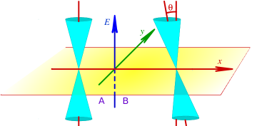
Figure 1: A schematic representation of the behavior of electrons when passing through a heterojunction of 2D Dirac materials, where electrons undergo quantum tunneling between regions with upright and tilted Dirac cones.

In order to accomplish this task, we can begin our study by considering a heterojunction formed by two different Dirac materials, each with distinct types of tilt in their energy bands, as illustrated in Fig. 1. As depicted in the figure, the mediums are labeled by $A$ and $B$, the Dirac cone on the left side ($x<0$) remains untilted ($\zeta_{A}=0$), while it exhibits tilt ($\zeta_{B}\neq 0$), on the right side ($x>0$). Consequently, the tilt velocity in Eq. (1) becomes a function of $x$ and can be expressed as

$$v_{t}(x)=v_{t}\Theta(x)=v_{t}\Big{\{}\begin{array}[]{lr}0,&\quad x<0,\\ 1,&\quad x>0,\end{array},$$ (4)

where $\Theta(x)$ denotes the Heaviside unit step function.

It is important to highlight that in our investigation, we specifically address the scenario with Dirac cones tilted in the $k_{x}$-direction, which is perpendicular to the interface. This configuration is distinct from cases where the tilt is parallel to the interface, as discussed in the literature Pattrawutthiwong01 .

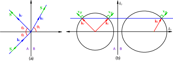
Figure 2: Reflection and transmission of the electron waves at the interface between two 2D materials for an oblique incidence: (a) Orientation of the wave vectors ${\bf k}_{i}$, ${\bf k}_{r}$ and ${\bf k}_{t}$ the pseudo-spin ${\bf S}$ at the interface, (b) The intersections of the Fermi surface and the Dirac cones in regions $A$ and $B$. The Dirac cones for the second region are tilted. ${\bf v}_{gi}$, ${\bf v}_{gr}$, and ${\bf v}_{gt}$ are the group velocities of the incident, reflected and transmitted waves, respectively.

We are interested in understanding the transmission properties across the interface between regions $A$ and $B$, as illustrated in Fig. 1. Before delving into the calculations of reflection and transmission coefficients, let us establish the boundary conditions by utilizing the continuity equation. In elementary quantum mechanics, it is well known that the probability density, $\rho$, and the probability current density, $\bf{J}$, satisfy the continuity equation:

$${\partial\rho\over\partial t}+\bf{\nabla}\cdot\bf{J}=0,$$ (5)

representing the conservation of the probability in a given system which is a fundamental concept in quantum mechanics. Now, assume that the Hamitonian describing the transport of an untilted Dirac fermion in a “hypothetical system” is given by $H=\sigma_{z}k_{z}=-i\sigma_{z}\partial/\partial z$. For this case, using the time dependent Schrödinger equation, it is easy to show that the continuity equation is satisfied with $\rho$ and ${\bf J}$ defined in terms of wavefunction $\psi$ as $\rho=\psi^{\dagger}\psi$ and ${\bf J}=(\psi^{\dagger}\sigma_{z}\psi){\bf e}_{z}$ in which ${\bf e}_{z}$ is the unit vector in $z$ direction. Also, in this case it is an easy practice to show that the wavefunction $\psi$ is continues everywhere even at the interface of two $2D$ Dirac mediums with untilted Dirac cones. This fact implies that, at the interface of these regions, we have $\psi_{A}=\psi_{B}$ where $\psi_{A}$ and $\psi_{B}$ refer to the electron wavefunctions in regions $A$ and $B$ at the interface, respectively. It should be mentioned that $\psi$, $\rho$ and $\bf{J}$ are all functions of the position $\bf{r}$ and time $t$, but for the sake of brevity, explicit display of this dependence has been avoided.

In similarity with what was stated above for the untilted Dirac fermions, the continuity equation remains hold for the tilted Dirac fermions obeying the Hamiltonian given in Eq. (1), if ${\bf J}$ is defined as ${\bf J}=J_{x}{\bf e}_{x}+J_{y}{\bf e}_{y}$ with $J_{x}=\psi^{\dagger}(v_{x}\sigma_{x}+v_{t}{\bf 1})\psi$ and $J_{y}=\psi^{\dagger}v_{y}\sigma_{y}\psi$. Consequently, if $J_{x}$ can be written as $J_{x}=\Psi^{\dagger}\sigma_{z}\Psi$, it can be concluded that $\Psi$ is continues everywhere including the interface of the regions. Specially, at the interface of the regions, we have:

$$\Psi_{A}=\Psi_{B},$$ (6)

which is a crucial point to continue the discussion.

With the above introduction we return to the main issue in question. A schematic representation of the considered system is depicted in Fig. 2. The figure illustrates two key aspects: (a) the orientation of the wave vectors ${\bf k}_{i}$, ${\bf k}_{r}$, ${\bf k}_{t}$, and the pseudo-spin ${\bf S}$ at the interface, and (b) the intersections of the Fermi surface and the Dirac cones in regions $A$ and $B$, with the cones in the second region being tilted. In part (a), the orientation of the wave vectors and the pseudo-spin at the interface is depicted, providing insight into the behavior of the wave vectors and the associated pseudo-spin at the interface. This orientation is crucial for understanding the dynamics of the system at the interface. In part (b), the intersections of the Fermi surface and the Dirac cones in regions $A$ and $B$ are shown, with particular emphasis on the tilted nature of the cones in the second region. This tilt has significant implications for the electronic properties in this region, and the figure serves to visually convey this important characteristic. The intersections of the Fermi surface and the Dirac cones are fundamental to the electronic structure and behavior of the material, and the tilt in the second region introduces additional complexity to the electronic properties, which is effectively captured in the figure.

If the probability current densities in regions $A$ and $B$ are represented by $\bf{J}_{A}$ and $\bf{J}_{B}$, respectively, the perpendicular components of these two vector quantities must be equal at the junction of the regions, that is: $J_{Ax}=J_{Bx}$. This condition implies that

$$\psi_{A}^{\dagger}(v_{A}\sigma_{x}+v_{At}{\bf 1})\psi_{A}=\psi_{B}^{\dagger}(v_{B}\sigma_{x}+v_{Bt}{\bf 1})\psi_{B}$$ (7)

in which $v_{A}$ and $v_{B}$ are the $x$ components of the electron velocities in regions $A$ and $B$, respectively.

A similar boundary condition has been derived for quantum transport in the Weyl semimetals of type II in Refs. Hashimoto01 and Witten01 . However, it is important to note two differences. First, in the mentioned references, the right side of the equation has been set equal to zero, which is due to the assumption of a closed boundary condition in those studies, but in the current research, the boundary condition is for the quantum transport of the massless Dirac fermions from the interface of the regions. The other is that in the mentioned studies, the similar boundary condition has been obtained by providing some different and a little complicated discussions, while in this research, the appropriate boundary condition has been deduced simply by employing the continuity condition.

Our attention is now directed towards expressing the continuity condition given in Eq. (7) as

$$\Psi_{A}^{\dagger}\sigma_{z}\Psi_{A}=\Psi_{B}^{\dagger}\sigma_{z}\Psi_{B},$$ (8)

in order to establish the continuity of $\Psi$ at the boundary of the regions as stated in Eq. (6). For this purpose, using a unitary transformation represented by the unitary operator of $U$ denoted as

$$U={1\over\sqrt{2}}(\sigma_{x}+\sigma_{z})={1\over\sqrt{2}}\Big{(}\begin{array}[]{cc}1&1\\ 1&-1\end{array}\Big{)},$$ (9)

it is possible to transform Eq. (7) to

$$\begin{split}v_{A}\psi_{A}^{\dagger}U^{\dagger}(\sigma_{z}&+\zeta_{A}{\bf 1})U\psi_{A}\\ &=v_{B}\psi_{B}^{\dagger}U^{\dagger}(\sigma_{z}+\zeta_{B}{\bf 1})U\psi_{B},\end{split}$$ (10)

where $\sigma_{z}=U^{\dagger}\sigma_{x}U$, and $\zeta_{A}$ and $\zeta_{B}$ denote the tilt parameters for mediums $A$ and $B$, correspondingly. The boundary condition represented in Eq. (8) can be expressed in its explicit matrix form as

$$v_{A}\psi_{A}^{\dagger}\Big{(}\begin{array}[]{cc}\zeta_{A}&1\\ 1&\zeta_{A}\end{array}\Big{)}\psi_{A}=v_{B}\psi_{B}^{\dagger}\Big{(}\begin{array}[]{cc}\zeta_{B}&1\\ 1&\zeta_{B}\end{array}\Big{)}\psi_{B}.$$ (11)

By converting this relation into the form given in Eq. (8) and considering Eq. (6), a continues quantity at the interface is obtained such as:

$$\begin{split}\sqrt{v_{A}}\Big{(}\begin{array}[]{cc}\sqrt{1+\zeta_{A}}&0\\ 0&\sqrt{1-\zeta_{A}}\end{array}\Big{)}U\psi_{A}\qquad\qquad\qquad\qquad\\ =\sqrt{v_{B}}\left(\begin{array}[]{cc}\sqrt{1+\zeta_{B}}&0\\ 0&\sqrt{1-\zeta_{B}}\end{array}\right)U\psi_{B}.\end{split}$$ (12)

A similar expression has been also derived in Ref. Hashimoto01 for theoretical study of the escape from black hole analogs in 2D materials.

Ultimately, when both sides of Eq. (12) are multiplied from the left by unitary matrix $U^{\dagger}$, the continuity condition of that component of ${\bf J}$ which is perpendicular to the interface at the junction of the regions is reduced accordingly as

$$M_{A}\psi_{A}=M_{B}\psi_{B},$$ (13)

where $M_{A}$ and $M_{B}$ are two $2\times 2$ matrices corresponding to the mediums of $A$ and $B$, respectively. The explicit matrix form of these matrices are given by

$$M_{A}=\Big{(}\begin{array}[]{cc}a_{A}&b_{A}\\ b_{A}&a_{A}\end{array}\Big{)},\quad{\rm and}\quad M_{B}=\Big{(}\begin{array}[]{cc}a_{B}&b_{B}\\ b_{B}&a_{B}\end{array}\Big{)}$$ (14)

where

$$\begin{split}a_{A}={1\over 2}\sqrt{v_{A}}\Big{(}\sqrt{1+\zeta_{A}}+\sqrt{1-\zeta_{A}}\Big{)},\\ b_{A}={1\over 2}\sqrt{v_{A}}\Big{(}\sqrt{1+\zeta_{A}}-\sqrt{1-\zeta_{A}}\Big{)}.\end{split}$$ (15)

Similarly, $a_{B}$, and $b_{B}$ have the same forms as those in Eq. (15), except that index $A$ should be replaced by $B$.

It is evident that if the tilt velocities in both regions are equal, i.e. $v_{A}=v_{B}$, it leads to $M_{A}=M_{B}$, resulting in the simplification of the boundary condition of Eq. (13) to $\psi_{A}=\psi_{B}$. This condition holds true even if $v_{A}=v_{B}=0$, which indicates no tilt in the $k_{x}$-direction (though tilt may still exist in the $k_{y}$-direction, as shown in Ref. Pattrawutthiwong01 ). However, for our current research, given the tilt in the direction perpendicular to the interface between regions $A$ and $B$, we will utilize the boundary condition provided in Eq. (13), as we will discuss it further.

Prior to concluding this subsection, we address the rotation of the “spin” or “pseudospin” state of the Dirac fermions in confronting with the interface of the regions at which a sudden change occurs in tilt. For the sake of simplicity in the calculations, we revert to the bases obtained after employing the unitary transformation represented in Eq. (9). In the specified bases, if the “spin” or “pseudospin” states of the Dirac fermions, in regions $A$ and $B$, are denoted by $\psi_{SA}$ and $\psi_{SB}$, respectively, by referring to Eq. (12), it is found that

$$\begin{split}\psi_{SB}=\sqrt{v_{A}/v_{B}}&\Big{(}\begin{array}[]{cc}\sqrt{1+\zeta_{B}}&0\\ 0&\sqrt{1-\zeta_{B}}\end{array}\Big{)}^{-1}\\ &\Big{(}\begin{array}[]{cc}\sqrt{1+\zeta_{A}}&0\\ 0&\sqrt{1-\zeta_{A}}\end{array}\Big{)}\psi_{SA}.\end{split}$$ (16)

Using the basic calculus, the above relation can be easily reduced to

$$\psi_{SB}=\Big{(}\begin{array}[]{cc}a_{S}&0\\ 0&b_{S}\end{array}\Big{)}\psi_{SA}.$$ (17)

where $a_{S}$ and $b_{S}$ are given by the following expressions:

$$a_{S}=\sqrt{v_{A}(1+\zeta_{A})\over v_{B}(1+\zeta_{B})},\quad{\rm and}\quad b_{S}=\sqrt{v_{A}(1-\zeta_{A})\over v_{B}(1-\zeta_{B})}.$$

We assume that the “spin” or “pseudospin” state $\psi_{SA}$ is given in terms of the spherical coordinates by

$$\psi_{SA}=\begin{pmatrix}\cos({\theta/2})\ e^{-i\phi/2}\\ \sin({\theta/2})\ e^{+i\phi/2}\end{pmatrix}.$$ (18)

This state is the eigenstate of ${\bf S}\cdot{\bf n}$ with eigenvalue of $+1/2$. Here, ${\bf S}$ denotes the “spin” or “pseudospin” operator and ${\bf n}$ is an arbitrary unit vector representing the direction associated with the polar and azimuthal angles of $\theta$ and $\phi$, respectively. Consequently, Eq. (17) leads to

$$\psi_{SB}=\Big{(}\begin{array}[]{c}a_{S}\cos(\theta/2)\ e^{-i\phi/2}\\ b_{S}\sin(\theta/2)\ e^{+i\phi/2}\end{array}\Big{)}.$$

In order to examine the “spin” or “pseudospin” direction of $\psi_{SB}$, the corresponding state can be rewritten as

$$\psi_{SB}=N\Big{(}\begin{array}[]{c}\cos({\theta_{S}/2})\ e^{-i\phi/2}\\ \sin({\theta_{S}/2})\ e^{+i\phi/2}\end{array}\Big{)},$$ (19)

where $N$ is a normalization factor, and

$$\theta_{S}=2\tan^{-1}\big{[}b_{S}\tan(\theta/2)/a_{S}\big{]}.$$ (20)

In other words, since $a_{S}$ and $b_{S}$ are real numbers, during the passage through the boundary, the polar angle of the spin relative to the axis along which the tilt occurs changes, while the azimuthal angle perpendicular to the tilt direction remains unchanged.

The above calculations demonstrate that at the interface of the two regions, the pseudo-spin direction remains in the $x-y$ plane, but its orientation with respect to the $x$-axis in the $x-y$ plane changes.

In the following, we examine quantum transport of the Dirac fermions in normal and oblique incidence of the electron wavefunction on the interface of two mediums as two separate cases.

II.2.1 Normal incidence analysis

Let us consider the case where an electron approaches to the interface from the left side of the considered heterojunction. To simplify our analysis, we will begin with the assumption of a normally incident electron, which implies $k_{y}=0$. We will also consider that the Dirac cone in region $B$ is in a sub-critically tilted phase $(0<\zeta_{B}<1)$. In this case, the wave functions can be expressed as:

$$\psi(x)=\begin{cases}e^{ik_{x}x}\Big{(}\begin{array}[]{c}1\\ 1\end{array}\Big{)}+re^{-ik_{x}x}\Big{(}\begin{array}[]{c}1\\ -1\end{array}\Big{)},&x<0,\\ t\Big{(}\begin{array}[]{c}1\\ 1\end{array}\Big{)}e^{ik_{x}x},&x>0,\end{cases}$$ (21)

where the first row is assumed as the electron wave function in region $A$ and the second row as the same in region $B$. $r$ and $t$ represent the reflection and transmission amplitudes, respectively. By applying the boundary conditions given in Eq. (13) at the interface assumed at $x=0$ and considering $\zeta_{A}=0$, the following coupled equations can be easily derived:

$$\begin{split}1+r=(\sqrt{1+\zeta_{B}})t,\\ 1-r=(\sqrt{1+\zeta_{B}})t,\end{split}$$ (22)

for which the solutions are

$$r=0,\qquad\text{and}\qquad t=1/\sqrt{1+\zeta_{B}}.$$ (23)

We can also calculate the transmission probability $T$, which is defined in terms of the incident and transmitted probability current densities denoted as $J_{i}$ and $J_{t}$, respectively,

$$T={J_{t}\over J_{i}}={J_{Bx}\over J_{Ax}}.$$ (24)

As discussed earlier, it is clear that the incident probability current density $J_{i}$ is $J_{Ax}=\psi_{A}^{\dagger}(v\sigma_{x})\psi_{A}=v$ and the transmitted probability current density $J_{t}$ is $J_{Bx}=\psi_{B}^{\dagger}(v_{x}\sigma_{x}+v_{t}{\bf 1})\psi_{B}=v$. Therefore, if the electron arrives to the interface with normal incidence, the probability of it passing through is 1, meaning $T=1$. This is often referred to as the Klein tunneling effect Dombey01 , which this result shows it occurs even in the presence of tilt in the energy band dispersion where $|t|\neq 1$.

It is interesting that if the traveling direction of the electrons is reversed, so that they incident from the tilt medium to the interface, there is still a possibility of complete tunneling.

It is worth noting that when $\zeta_{B}>1$, it is impossible to express the wave function for region $B$ as given in Eq. (21) because a particle with a group velocity moving from right to left cannot be found in this region. Additionally, if a particle crosses the boundary, it cannot escape, resembling the event horizon of a black hole. This scenario is interesting and reminiscent of the behavior near a black hole’s event horizon.

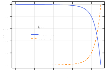
Figure 3: The probability of reflection and transmission for various incident angles as the Dirac fermions enter the region with tilted Dirac cones from the region without tilt (region $A$ to $B$).

II.2.2 Oblique incidence analysis

Let us now explore the oblique incidence at the interface between regions $A$ and $B$ as a second but more general case. We consider an incoming electron with a given wavevector of ${\bf k}_{i}$, which is reflected with wavevector ${\bf k}_{r}$ in region $A$, and is transmitted into region $B$ with a wavevector of ${\bf k}_{t}$. This scenario is more complex than the normal incidence case, as the wave vectors and the angles of incidence, reflection, and transmission are involved.

Referring to the angles illustrated in Fig. 2, we can establish the wavevectors as ${\bf k}_{\alpha}=(k_{\alpha x},k_{\alpha y})=k_{\alpha}(\beta\cos\theta_{\alpha},\sin\theta_{\alpha})$ for $\alpha=i,~{}r,~{}t$, in which indices $i$, $r$ and $t$ refer to the incident, reflected and transmitted waves, respectively. $k_{\alpha}$ is the norm of ${\bf k}_{\alpha}$ and $\beta$ is $-1$ for the reflected and is $+1$ for the incident and transmitted wave vectors. Given the conservation of energy $E$ and momentum projection $k_{y}$, the component which is parallel to the interface, we can immediately conclude $k_{r}=k_{i}$, $\theta_{r}=\theta_{i}$, $k_{ty}=k_{iy}$,

$$\theta_{t}=\cot^{-1}{\Big{(}{{-\zeta_{B}+\sqrt{1-(1-\zeta_{B}^{2})\sin^{2}{\theta_{i}}}\over(1-\zeta_{B}^{2})\sin\theta_{i}}\Big{)}}},$$ (25)

and $k_{tx}$ reads as

$$k_{tx}={-\zeta_{B}E+\sqrt{\zeta_{B}^{2}E^{2}+(1-\zeta_{B}^{2})k_{ix}^{2}}\over 1-\zeta_{B}^{2}}.$$ (26)

The associated wave functions to the incident, reflected and transmitted electrons can be respectively expressed as:

$$\begin{split}\psi_{i}({\bf r})&=\Big{(}\begin{array}[]{c}1\\ e^{i\theta_{i}}\end{array}\Big{)}e^{i{\bf k}_{i}\cdot\bf{r}},\\ \psi_{r}({\bf r})&=\Big{(}\begin{array}[]{c}1\\ -e^{-i\theta_{r}}\end{array}\Big{)}e^{i{\bf k}_{r}\cdot\bf{r}},\\ \psi_{t}({\bf r})&=\Big{(}\begin{array}[]{c}1\\ e^{i\theta_{t}}\end{array}\Big{)}e^{i{\bf k}_{t}\cdot\bf{r}}.\end{split}$$ (27)

These equations allows us to find the wave functions in both regions as

$$\begin{split}\psi_{A}({\bf r})&=\psi_{i}({\bf r})+r\psi_{r}({\bf r}),\quad\text{for}\quad x<0,\\ \psi_{B}({\bf r})&=t\psi_{t}({\bf r}),\qquad\qquad\ \ \text{for}\quad x>0.\end{split}$$ (28)

Inserting these wavefunctions into Eq. (13), the following relations between the reflection and transmission amplitudes are drivable:

$$\begin{split}1+r=a_{B}t+b_{B}te^{i\theta_{t}},\\ e^{i\theta_{i}}-re^{-i\theta_{i}}=b_{B}t+a_{B}e^{i\theta_{t}}.\end{split}$$ (29)

After some straightforward algebra, the solutions for $r$ and $t$ are obtained as:

$$\begin{split}t&={2\cos\theta_{i}\over 2a_{B}\cos\theta_{i}+b_{B}(1+e^{i(\theta_{t}-\theta_{i})})},\\ r&=t(a_{B}+b_{B}e^{i\theta_{t}})-1.\end{split}$$ (30)

For this case, the subsequent step involves calculating the reflection and transmission coefficients, $R$ and $T$. This includes calculating the ratios of $J_{r}/J_{i}$ and $J_{t}/J_{i}$. The perpendicular probability flux in region $A$, $J_{Ax}$, can be expressed as:

$$J_{Ax}=v\psi_{A}^{\dagger}\sigma_{x}\psi_{A}=J_{i}+J_{r},$$ (31)

where $J_{i}$ and $J_{r}$ are contributions from the incident and reflected wavefunctions, respectively. Subsequently, these contributions are derivable as

$$\begin{split}J_{i}&=2v|1+r|\cos{(\theta_{i}-\delta_{1})},\\ J_{r}&=2v|r(1+r)|\cos{(\theta_{i}+\delta_{2})},\end{split}$$ (32)

where, $\delta_{1}$ and $\delta_{2}$ are the phases associated with expressions $1+r$ and $r^{*}(1+r)$, respectively. Here the asterisk refers to complex conjugate.

Similarly, the probability flux transmitted perpendicular, $J_{t}$, reads

$$J_{t}=v\psi_{B}^{\dagger}(\sigma_{x}+\zeta_{B}{\bf 1})\psi_{B}=2|t|v(\zeta_{B}+\cos\theta_{t}).$$ (33)

Consequently, $R$ and $T$ are determined as

$$\begin{split}R&={J_{r}\over J_{i}}={|r|\cos{(\theta_{i}+\delta_{2})}\over\cos{(\theta_{i}-\delta_{1})}},\\ T&={J_{t}\over J_{i}}={|t|^{2}[\cos{\theta_{t}+\zeta_{B}}]\over 2|1+r|\cos{(\theta_{i}-\delta_{1})}}.\end{split}$$ (34)

In Fig. 3, the behavior of both the reflection and transmission probabilities, $R$ and $T$, as functions of incident angle $\theta_{i}$ is visually represented. The phenomenon of Klein tunneling remains prominent for incident angles less than $50^{\circ}$, with $T$ reaching nearly $1$. However, as $\theta_{i}$ exceeds $50^{\circ}$, the probability of reflection becomes notably significant. It is worth noting that in this figure, the tilt parameter is assumed to be $\zeta_{B}=0.4$. The change in these probabilities with the incident angle $\theta_{i}$ and the tilt parameter $\zeta_{B}$ provides valuable insights into the quantum behavior of the system.

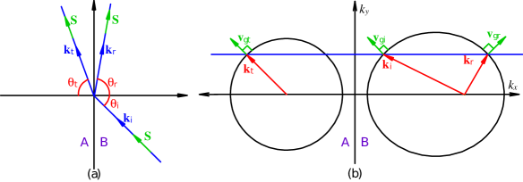
Figure 4: Same as figure 2, but for incidence of Dirac fermions from the region with tilted cones to the region without tilting

Before closing this subsection, it is interesting to ask what will happen if the incident direction is reversed from right to left on the hetrojunction. To explore the scenario of transmission from the tilted side to the untilted one (reversing the incident direction), we need to consider the corresponding angles and wavevectors, which are depicted in Fig. 4. By applying the conservation laws discussed earlier, we can numerically determine $\theta_{t}$ using the following relation:

$$\theta_{i}=\cot^{-1}\Big{(}{-\zeta_{B}-\sqrt{1-(1-\zeta_{B}^{2})\sin^{2}{\theta_{t}}}\over(1-\zeta_{B}^{2})\sin\theta_{t}}\Big{)},$$ (35)

and then use the result to determine $\theta_{r}$ as

$$\theta_{r}=\cot^{-1}\Big{(}{-\zeta_{B}+\sqrt{1-(1-\zeta_{B}^{2})\sin^{2}{\theta_{t}}}\over(1-\zeta_{B}^{2})\sin\theta_{t}}\Big{)}.$$ (36)

This procedure comes from the fact that obtaining the closed analytical form for $\theta_{t}$ from Eq. (35), is complicated and difficult.

The previous analysis can be extended to determine the reflection and transmission probabilities for this case too. For $\zeta_{B}=0.4$, Fig. 5 displays the graphical representations of computed $R$ and $T$ as functions of the incident angle, $\theta_{i}$. The overall behavior is both qualitatively and quantitatively different from the previous case. The significant point that we get from the comparison of Figs. 3 and 5 is that the behavior of Dirac fermions at the boundary of two materials with different tiling depends on the incident direction. In the incidence from the untilted region to the tilted region, for an angular range of 0 to 50 degrees, the probability of the quantum Klein tunneling is perfect, but it is not the case in inverse. Also, another significant difference that can be seen in Fig. 5 is the existence of a critical incident angel for the case in which Dirac fermions entering from the tilted region to the region with upright cones. In Fig. 5, this angle is shown by $\theta_{c}$. In optics terminology, this angle refer to the specific angle of incidence that results in an angle of refraction of $90^{\circ}$, beyond which total internal reflection occurs. In fact, for incidence angles greater than  $\theta_{c}$, entry into region $A$ becomes prohibited. This angle is obtained by setting $\theta_{t}$ equal to $90^{\circ}$ in Eq. (35), for which the result is $\theta_{c}=\cot^{-1}\big{(}-2\zeta_{B}/(1-\zeta_{B}^{2})\big{)}$. The critical angle $\theta_{c}$, which introduces an additional constraint on the system is a key feature of the considered configuration, and the figure effectively conveys this information. For the case corresponding to Figs. 2 and 3, this critical angle is absolutely absent.

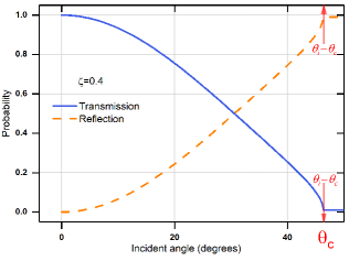
Figure 5: Same as figure 3, but for incidence of Dirac fermions from the region with tilted cones to the region without tilting. In this case there exists a critical angle, $\theta_{c}\simeq 46.4^{\circ}$, for which the fermion waves are totally reflected into the tilted material.

Another important item to address in this subsection is the angular amount of the rotation of the pseudospin of the massless Dirac fermions in crossing the boundary of the Dirac materials with different tilts. In Fig. 6, a comprehensive analysis of this significant issue has been conducted. In this figure the left column is for crossing from $A$ to $B$ and the other is for the reversed crossing. Also the first row is produced to show the amount of the spin rotation, $\Delta\theta_{S}=\theta_{S}-\theta$, as a function of the incident angle, $\theta_{i}$, for some fixed values of $\zeta_{B}$. The second row demonstrates $\Delta\theta_{S}$ as a function of tilt parameter $\zeta_{B}$, for some fixed values of $\theta_{i}$. All the graphs are plotted by employing Eq. (20). As is seen from the figure, in both cases, $\Delta\theta_{S}$ is almost an increasing function of $\theta_{i}$ and/or $\zeta_{B}$. In panel (a), The slope of the changes is high at the beginning, but at larger angles, this slope is adjusted and even turns slightly downward. For entering from $B$ to $A$, as it has been explained in the discussion provided on Fig. 5, for each fixed value of $\zeta_{B}$, there exists a critical incident angle at which the electron wave is totally reflected into the tilted medium. These critical angles are marked with arrows in panel (b). In panels (c) and (d), the slope of changes is absolutely positive and increasing. Panel (d) shows that for any given incident angle, there exists a certain value of the tilt parameter, beyond which the electronic wave is entirely reflected into the medium $B$. For different values of $\theta_{i}$, these critical values are labeled with $\zeta_{c}$ and are shown with arrows in this panel. In the first row, $\theta_{i}$ has changed from zero to $\pi/2$ or to $\theta_{c}$. If the interval of $\theta_{i}$ changes is taken to be symmetrical, for example $[-\pi/2,+\pi/2]$ or $[-\theta_{c},\theta_{c}]$, the graphs will be symmetrical with respect to the vertical axis, that is, $\Delta\theta_{s}$ is an even function of $\theta_{i}$. Of course, this feature is confirmed by current calculations and it can be found out from Figs. 2 and 4. It is worthy to mention that, in all the considered cases, there is no observation of a change in the sign of the pseudospin of the massless electrons.

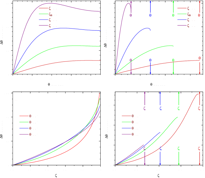
Figure 6: The change in angular orientation of the pseudospin of massless Dirac electrons, denoted as $\Delta\theta_{S}$, as they cross the interface between two Dirac materials having different tilt parameters: The left column is for the setup presented in Fig. 2 and the other for the same in Fig. 4. The first row displays $\Delta\theta_{S}$ as a function of $\theta_{i}$ for some fixed values of $\zeta_{B}$ and the second row demonstrates it as a function of $\zeta_{B}$ but for several fixed values of $\theta_{i}$. In the right column the critical incident angle and tilt parameter are denoted by $\theta_{c}$ and $\zeta_{c}$, respectively.

II.3 Double interface heterojunction

Now, let us explore a heterojunction with double interfaces, as depicted in Fig. 7. This setup comprises three regions, denoted as $A$, $B$, and $C$. Regions $A$ and $C$ contain untilted Dirac cones, while the middle region, region $B$, features a tilted Dirac cone, represented by $\zeta_{B}$. The middle slab’s thickness containing the subcritical Dirac cones is denoted as $\ell$. For the specified three-medium structure, depicted in Fig. 7, the corresponding wave functions for the regions can be written as

$$\psi(x)=\begin{cases}\Big{(}\begin{array}[]{c}1\\ e^{i\theta_{i}}\end{array}\Big{)}e^{i{\bf k}_{i}\cdot\bf{r}}+r\Big{(}\begin{array}[]{c}1\\ e^{i\theta_{r}}\end{array}\Big{)}e^{i{\bf k}_{r}\cdot\bf{r}},&\text{for }x<0,\\ D_{1}\Big{(}\begin{array}[]{c}1\\ e^{i\theta_{1}}\end{array}\Big{)}e^{i{\bf k}_{1}\cdot\bf{r}}+D_{2}\Big{(}\begin{array}[]{c}1\\ e^{i\theta_{2}}\end{array}\Big{)}e^{i{\bf k}_{2}\cdot\bf{r}},&\text{for }0<x<\ell,\\ t\Big{(}\begin{array}[]{c}1\\ e^{i\theta_{t}}\end{array}\Big{)}e^{i{\bf k}_{t}\cdot\bf{r}},&\text{for }x>\ell,\end{cases}$$ (37)

where $D_{1}$ and $D_{2}$ are two constant coefficients, ${\bf k}_{1}$ and ${\bf k}_{2}$ are the wave vectors of the traveling and reflected waves in the middle region, and angles $\theta_{1}$ and $\theta_{2}$ indicate the orientation of these wave vectors with respect to the direction of tilting. The indicated angles along with the components of the wave vectors such as $k_{1x}$, $k_{2x}$, and $k_{tx}$ can be obtained using the energy and momentum conservation laws as in the previous section. These results obtained from the mentioned procedure are

$$\theta_{1}=\cot^{-1}{\Big{(}{-\zeta_{B}-\sqrt{1-(1-\zeta_{B}^{2})\sin^{2}{\theta_{t}}}\over(1-\zeta_{B}^{2})\sin\theta_{t}}\Big{)}},$$ (38)

$$\theta_{2}=\cot^{-1}{\Big{(}{-\zeta_{B}+\sqrt{1-(1-\zeta_{B}^{2})\sin^{2}{\theta_{t}}}\over(1-\zeta_{B}^{2})\sin\theta_{t}}\Big{)}},$$ (39)

$$k_{Ax}={-\zeta_{B}+\sqrt{1-(1-\zeta_{B}^{2})\sin^{2}{\theta_{t}}}\over 1-\zeta_{B}^{2}},\qquad\qquad$$ (40)

$$k_{Bx}={-\zeta_{B}-\sqrt{1-(1-\zeta_{B}^{2})\sin^{2}{\theta_{t}}}\over 1-\zeta_{B}^{2}},\qquad\qquad$$ (41)

and

$$k_{tx}={E\over v_{x}}\cos\theta_{t}.$$ (42)

To obtain the coefficients $D_{1}$, $D_{2}$ and the reflection and transmission amplitudes $r$, and $t$, we need to employ the boundary condition given in Eq. (13) on both interfaces assumed at $x=0$ and $x=\ell$. The corresponding equations read

$$\psi_{A}(0)=M_{B}\psi_{B}(0),$$ (43)

$$M_{B}\psi_{B}(\ell)=\psi_{C}(\ell).$$ (44)

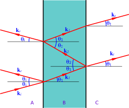
Figure 7: Incident Dirac fermion wave with a wavevector of ${\bf k}_{i}$ strikes the slab of an tilted fermion Dirac material (region B) placed between two untilted Dirac mediums (regions A and C), giving rise to the reflected and transmitted Dirac fermion waves with wave vectors of ${\bf k}_{r}$ and ${\bf k}_{t}$, respectively.

After performing the necessary calculations, the reflection and transmission probabilities, $R$ and $T$, can be derived. Although the closed but complex forms of these expressions are not provided here, they can be utilized to examine the behavior of Dirac fermions in confronting with the interfaces. As an example, the changes of $T$ in terms of the middle slab’s thickness, for two cases of incidence from left to right and incidence from right to left are visualized in Fig. 8. In this figure, panels $(a)$ and $(b)$ illustrate the behavior of the transmission probability for the specified cases, respectively. As is seen, the plots exhibit two different but nearly opposite behaviors. In other words, in regions where the probability of transmission from left to right is nonzero, the probability of transmission from right to left is perfect and vice versa. This antisymmetry is so clear that the graphs can be considered nearly complementary to each other. Another important point is that the transmission probability is a periodic function of the thickness of the middle region with the subcritical tilted Dirac cones, and the period of oscillation depends on the tilt parameter of this medium, $\zeta_{B}$. Also, for certain thicknesses of the middle slab, the probability of quantum tunneling of the Dirac fermions inside the slab is perfect. For both considered cases, these thicknesses are in some continuous and wide ranges. Another point is that the thicknesses in which the Klein tunneling occurs are independent of the incidence angles, so that for all the angles shown in the figure in both cases, Klein tunneling occurs in the same range of thickness. With the features listed above, it seems that tuning the length of the middle slab to observe this phenomenon experimentally probably is not so difficult.

As expected and the above studies confirm, when Dirac fermions cross the interface between two materials with different tilts, their behavior can indeed be different depending on the direction of traversal. The resulting phenomena can have implications for novel electronic devices and fundamental research in condensed matter physics.

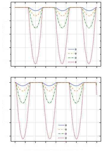
Figure 8: Quantum tunneling probability of Dirac fermions within a slab with thickness $\ell$ for configuration illustrated in Fig. 7 in two different situations: (a) Forward traveling (left to right) and (b) Reverse traveling (right to left). The transmission probability for various incident angles is plotted against the slab’s thickness, $\ell$. In both cases $\zeta_{B}=0.4$.

III Summary and Conclusion

In this study, we have thoroughly investigated the profound implications of tilted Dirac cones on the quantum transport properties of two-dimensional (2D) Dirac materials. Our research has focused on materials with tilted Dirac cones, where the anisotropic and tilted nature of the cones introduces additional complexity and richness to their electronic properties. The investigation began by considering a heterojunction of 2D Dirac materials, where electrons undergo quantum tunneling between regions with upright and tilted Dirac cones. We have provided a comprehensive theoretical investigation into the impact of tilted Dirac cones on electron transmission and pseudospin dynamics in 2D materials. Our study has revealed several key findings. We have derived boundary conditions governing reflection and transmission between two regions characterized by different tilts, and quantified the spin rotation at the interface. Furthermore, we have investigated the probabilities of electron reflection and transmission during the transition from a non-tilted region to a tilted one. Our results have demonstrated that the probability of massless electron transmission through a tilted region exhibits a periodic dependence on the width of an intermediate region, with this periodicity being independent of the incident angle. Importantly, we have observed that, for sufficiently large region widths, the transmission probability approaches unity. Additionally, we have highlighted the asymmetry of transmission probabilities between left-to-right and right-to-left directions.

Electrons transmitted through an interface across which the tilting parameter abruptly changes undergo a rotation of its pseudospin. In the case of spin-orbit coupled Dirac cones, such as those in the surface of topological insulators, this would imply that the interface is capable of rotating the incoming spins. Although in the present study we assumed that the tilt parameter changes abruptly (and so does the pseudo-spin rotation), in a generic setting where the tilt parameter changes smoothly it is again expected to have a smooth rotation of spin orientation. Since the tilt parameter is a proxy for spacetime metric Volovik01 ; Volovik02 ; Volovik03 ; Mola01 ; Mola02 this can be considered as an example of a gravitomagnetic effect, where spatial variation of certain metric entries may have an effect that effectively looks like a ”magnetic field” Ryder01 .

The implications of our research extend to the ongoing efforts to manipulate and precisely tune the tilt in Dirac materials. Furthermore, our study has shed light on the broader implications of tilted Dirac cones, particularly in less symmetric Dirac materials, where the Coulomb interaction can give rise to even more exotic phenomena. Moreover, we have delved into the theoretical exploration of the excitonic transition in 2D tilted cones to understand the electron-hole pairing instability as a function of tilt, providing valuable insights into the chiral excitonic instability of such systems. In conclusion, our study has significantly advanced the understanding of quantum transport phenomena in 2D materials with tilted Dirac cones. The insights gained from this research have the potential to inform the development of novel quantum devices and pave the way for further theoretical and experimental investigations into the unique electronic properties of materials with tilted Dirac cones.

References

- (1) K. S. Novoselov, A. K. Geim, S. V. Morozov, D. Jiang, Y. Zhang, S. V. Dubonos, I. V. Grigorieva, and A. A. Firsov, Science 306, 666-669 (2004).
- (2) A. H. Castro Neto, F. Guinea, N. M. R. Peres, K. S. Novoselov, and A. K. Geim, Rev. Mod. Phys. 81, 109 (2009).
- (3) N. Dombey and A. Calogeracos, Phys. Rep. 315, 41 (1999).
- (4) M. I. Katsnelson, K. S. Novoselov, and A. K. Geim, Nat. Phys. 2, 620 (2006).
- (5) E. Ghanbari-Adivi, M. Soltani, M. N. Sheikhali, Quantum Inf. Process. 15, 2377-2391 (2016)
- (6) C. C. Liu, W. Feng, and Y. Yao, Phys. Rev. Lett. 107, 076802 (2011).
- (7) X. Qian, J. Liu, L. Fu, and J. Li, Science 346, 1344 (2014).
- (8) H. Y. Lu, A. S. Cuamba, S. Y. Lin, L. Hao, R. Wang, H. Li, Y. Y. Zhao, and C. S. Ting, Phys. Rev. B 94, 195423 (2016).
- (9) S. Li, Y. Liu, Z. M. Yu, Y. Jiao, S. Guan, X. L. Sheng, Y. Yao, and S. A. Yang, Phys. Rev. B 100, 205102 (2019).
- (10) G. E. Volovik, JETP Lett. 114, 236 (2021).
- (11) G. E. Volovik and K. Zhang, J. Low Temp. Phys. 189, 276 (2017).
- (12) G. E. Volovik, Phys. Usp. 61, 89 (2018).
- (13) A. A. Soluyanov, D. Gresch, Z. Wang, Q. Wu, M. Troyer, X. Dai, and B. A. Bernevig, Nature (London) 527, 495 (2015).
- (14) Y. Yekta, H. Hadipour, and S. A. Jafari, Commun. Phys. 6, 46 (2023).
- (15) M. O. Goerbig, J. N. Fuchs, G. Montambaux, and F. Piechon, Phys. Rev. B 78, 045415 (2008).
- (16) M. Trescher, B. Sbierski, P. W. Brouwer, and E. J. Bergholtz, Phys. Rev. B 91, 115135 (2015).
- (17) J. F. Steiner, A. V. Andreev, and D. A. Pesin, Phys. Rev. Lett. 119, 036601 (2017).
- (18) Sh. H. Zhang, W. Yang, Phys. Rev. B 97, 235440 (2018).
- (19) X. Zhou, Phys. Rev. B 100, 195139 (2019) .
- (20) A. A. Zyuzin and R. P. Tiwari, JETP Lett. 103, 717 (2016).
- (21) Q. Ma, S. Y. Xu, C. K. Chan, C. L. Zhang, G. Chang, Y. Lin, W. Xie, T. Palacios, H. Lin, S. Jia, P. A. Lee, P. Jarillo-Herrero, and N. Gedik, Nat. Phys. 13, 842 (2017).
- (22) A. Wild, E. Mariani, and M. E. Portnoi, Phys. Rev. B 105, 205306 (2022).
- (23) C. Y. Tan, J. T. Hou, C. X. Yan, H. Guo, and H. R. Chang, Phys. Rev. B 106, 165404 (2022).
- (24) Z. Jalali-Mola and S. A. Jafari, Phys. Rev. B 100, 075113 (2019).
- (25) Z. Jalali-Mola and S. A. Jafari, Phys. Rev. B 104, 085152 (2021).
- (26) Y. Lu, D. Zhou, G. Chang, S. Guan, W. Chen, Y. Jiang, J. Jiang, X. S. Wang, S. A. Yang, Y. P. Feng, Y. Kawazoe, and H. Lin, NPJ Comput. Mater. 2, 16011 (2016).
- (27) Y. J. Long, L. X. Zhao, L. Shan, Z. A. Ren, J. Z. Zhao, H. M. Weng, X. Dai, Z. Fang, C. Ren, and G. F. Chen, Phys. Rev. B 95, 125417 (2017).
- (28) E. Pattrawutthiwong, W. Choopan, W. Liewrian, Phys. Lett. A 393, 127154 (2021).
- (29) K. Hashimoto and Y. Matsuo, Phys. Rev. B 102, 195128 (2020).
- (30) E. Witten, Riv. Nuovo Cim. 39, 313370 (2016).
- (31) L. Ryder, Introduction to General Relativity (Cambridge University Press, 2020).