State-action control barrier functions: Imposing safety on learning-based control with low online computational costs

Abstract

Learning-based control with safety guarantees usually requires real-time safety certification and modifications of possibly unsafe learning-based policies. The control barrier function (CBF) method uses a safety filter containing a constrained optimization problem to produce safe policies. However, finding a valid CBF for a general nonlinear system requires a complex function parameterization, which in general, makes the policy optimization problem difficult to solve in real time. For nonlinear systems with nonlinear state constraints, this paper proposes the novel concept of state-action CBFs, which not only characterize the safety at each state but also evaluate the control inputs taken at each state. State-action CBFs, in contrast to CBFs, enable a flexible parameterization, resulting in a safety filter that involves a convex quadratic optimization problem. This, in turn, significantly alleviates the online computational burden. To synthesize state-action CBFs, we propose a learning-based approach exploiting Hamilton-Jacobi reachability. The effect of learning errors on the effectiveness of state-action CBFs is addressed by constraint tightening and introducing a new concept called contractive CBFs. These contributions ensure formal safety guarantees for learned CBFs and control policies, enhancing the applicability of learning-based control in real-time scenarios. Simulation results on an inverted pendulum with elastic walls validate the proposed CBFs in terms of constraint satisfaction and CPU time.

I Introduction

Learning-based control methods have demonstrated extensive success across many applications, such as autonomous vehicles [1] and robot manipulation [2]. Both supervised learning and reinforcement learning (RL) have been widely used for controller synthesis. However, learning-based controllers may provide unsafe control actions that result in undesirable or even destructive effects on the system. In control systems, safety means that the trajectories of the closed-loop system should satisfy state and input constraints for the entirety of the system’s evolution. The lack of safety guarantees limits the ability of learning-based control to achieve safety-critical tasks.

There has been an increasing interest in designing strategies to make learning-based controllers safe. Among the available methodologies including penalty methods [3], constraint elimination [4], and using invariant sets [5, 6], using control-barrier functions (CBFs) [7, 8] for safe controller synthesis is a universal and convenient approach. CBFs are energy-based functions and use their sub-level sets to characterize the safety of the dynamical system, avoiding the use of complex invariant set representations. Given any learning-based controller without safety considerations, an online optimization problem, called a safety filter, is then solved to find the closest safe input to this controller, while safety is gained by adding a constraint based on a CBF into the optimization problem.

In the realm of CBF-based methodologies, a prominent limitation is the absence of universally applicable techniques for generating valid CBFs, thereby necessitating reliance on manually designed or problem-specific CBFs. For some particular kinds of systems such as linear, piecewise affine [9], or polynomial systems [10], CBFs can be computed by solving convex optimization problems. For nonlinear systems with general constraints, using learning-based algorithms accompanied by advanced function approximators to estimate CBFs has been explored in several contexts. Roughly, there are four kinds of methods to learn CBFs: the optimization-based method [11], the learner-verifier method [12], the Hamilton-Jacobi (HJ) reachability method [13], and the predictive safety filter method [14, 15]. The first two methods can be conservative, i.e., the learned safe set can be a small subset of the maximal controlled invariant set. In comparison, the HJ reachability method relies on the dynamic programming principle to approximate the maximal controlled invariant set iteratively, while the predictive safety filter method is based on a receding-horizon open-loop optimal control problem to implicitly determine the safe set, which also converges to the maximal controlled invariant set as the horizon goes to infinity [16]. A comprehensive comparison of HJ reachability, predictive safety filters, and CBFs can be found in [17].

No matter how the CBF is learned, to control a given system with safety guarantees, it is inevitable to solve an online optimization problem with CBF-based constraints, which is usually non-convex for discrete-time nonlinear systems [18]. To obtain a satisfactory approximation accuracy, sophisticated function approximators such as deep neural networks (NNs) are commonly used to parameterize the CBF [14, 7]. However, this will inherently cause non-convexity and increase the complexity of the optimization problem. As a result, the increased online computational load makes the CBF-based approach unsuitable for situations where fast computation of control inputs is required. Besides, the effect of approximation errors on the validity of the learned CBFs and the resulting control policies has not yet been addressed, as highlighted in [7].

This paper contributes to the state of the art in the following aspects. To impose safety on nonlinear systems at low online computational costs, we propose the novel concept of state-action CBFs, the zero sub-level sets of which can be used in the safety filter to generate a safe policy. Compared to standard CBFs, state-action CBFs allow for a flexible parameterization so that the resulting safety filter contains a convex quadratic optimization problem. Consequently, the online computation burden is greatly eased. To analyze the effect of approximation errors on learned CBFs, we propose a constraint tightening approach and introduce a novel concept of contractive CBFs. When learning such CBFs, the invariance property of CBFs can be retained, despite the presence of approximation errors. We also explore the connection between state-action CBFs and (contractive) CBFs, and develop a new learning-based method to approximate state-action CBFs. As a result, the safety of the policy filtered by state action CBFs is preserved for a sufficiently small approximation error.

II Preliminaries and problem formulation

II-A Preliminaries

We consider a deterministic discrete-time nonlinear system

$$x_{t+1}=f\left(x_{t},u_{t}\right),\quad t=0,1,\ldots,$$ (1)

where $x_{t}\in\mathcal{X}\subseteq\mathbb{R}^{n_{x}}$ and $u_{t}\in\mathcal{U}\subseteq\mathbb{R}^{n_{u}}$ are the state and the input at time step $t$, and $f(\cdot,\cdot):\mathcal{X}\times\mathcal{U}\to\mathcal{X}$ is a continuous function satisfying $f(0,0)=0$. We consider a constrained optimal control problem in which the states and inputs should satisfy time-invariant constraints: $x_{t}\in X:=\{x\in\mathcal{X}|h(x)\leq 0\}$ and $u_{t}\in U\subseteq\mathcal{U}$. Here, $h(\cdot):\mathcal{X}\to\mathbb{R}$ is a continuous function that defines the state constraint. Throughout the paper, we assume that we completely know $f$. Besides, we assume that $X$ is compact and that $U$ is a polytope.

The control objective is to regulate a redefined control policy, e.g., a policy learned by reinforcement learning or a policy that approximates model predictive control (MPC) [19], so that the safety of the system is ensured.

II-B Control barrier functions

To achieve the objective, we need to design a control policy that can ensure constraint satisfaction at all time steps. A set of states for which such a policy exists, needs to be defined. Usually, this class of sets is called controlled-invariant sets or safe sets. For high-dimensional systems, however, some controlled-invariant sets could have complex representations, making the controller synthesis difficult. A CBF uses the sub-level set of a scalar function to conveniently define the safe set.

Definition 1 (Control barrier function)

A continuous function $B(\cdot):\mathcal{X}\to\mathbb{R}$ is called a control barrier function (CBF) with a corresponding safe set $\mathcal{S}_{B}:=\left\{x\in\mathbb{R}^{n_{x}}|B(x)\leq 0\right\}\subseteq\mathcal{X}$, if $\mathcal{S}_{B}$ is non-empty,

$$h(x)\leq 0,\;\forall x\in\mathcal{S}_{B},$$ (2)

and

$$\min_{u\in U}B(f(x,u))\leq 0,\;\forall x\in\mathcal{S}_{B}.$$ (3)

Furthermore, a CBF is called an exponential CBF if it satisfies (2) with 0 replaced by $B(x)$ and if there exists a $\beta\in(0,1)$ such that

$$\min_{u\in U}B(f(x,u))\leq\beta B(x),\;\forall x\in\mathcal{S}_{B}.$$ (4)

Condition (2) is equivalent to $\mathcal{S}_{B}\subseteq X$, which is usually assumed in literature [18]. With a CBF available, one generate a safe control policy in $\mathcal{S}_{B}$ by using the following optimization-based approach:

$$\pi_{\mathrm{safe}}(x)=\arg\min_{u\in U} \;||u-\pi_{0}(x)||_{2}$$

$$\mathrm{s.t.} B(f(x,u))\leq 0,\;\mathrm{if}\;B\;\mathrm{satisfies}\;\eqref{CBF}$$

$$\mathrm{or}\;B(f(x,u))\leq\beta B(x),\;\mathrm{if}\;B\;\mathrm{satisfies}\;\eqref{CBFex},$$ (5)

which serves as a safety filter [5] for any unsafe policy $\pi_{0}$. The definition of a safe policy is formally given as follows.

Definition 2

A policy $\pi(\cdot):\mathcal{X}\to\mathcal{U}$ is safe in $\mathcal{S}\subseteq X$ for system (1) under the state and input constraints $x\in X,\;u\in U$, if $\pi(x)\in U,\;\forall x\in\mathcal{S}$, and for any initial state in $\mathcal{S}$, the state trajectory of (1) steered by $\pi$ will always stay in $\mathcal{S}$.

For general nonlinear systems with state and input constraints, synthesizing a non-conservative CBF is a difficult task. To deal with this issue, using advanced function approximators to learn a CBF certificate has received much attention. One can see [7] for a comprehensive survey.

II-C Problem formulation

Problem P1: high online computational complexity. One main limitation of (II-B) is that it needs to solve a usually non-convex optimization problem in real time. If a CBF is represented by a complex function approximator $B_{\theta}(\cdot)$ with the parameter $\theta$, solving (II-B) may take much online computation time and result in very sub-optimal solutions. Even if a convex $B_{\theta}$ is formed, the constraint in (II-B) could be non-convex due to the nonlinearity of $f$.
Problem P2: effects of approximation errors. Another limitation of (II-B) is that the approximation error of $B(\cdot)$ may affect the safety of the system controlled by the optimizer of (II-B) with $B(\cdot)$ replaced by $B_{\theta}(\cdot)$. Besides, the recursive feasibility of (II-B) is also not guaranteed with $B_{\theta}(\cdot)$.

III State-action control barrier function

To deal with Problem P1, motivated by Q-learning in RL [20], we propose a novel safety filter in the following form:

$$\pi_{\mathrm{safe}}(x)=\arg\min\{||u-\pi_{0}(x)||_{2},\;\mathrm{s.t.}\;u\in U,\;Q(x,u)\leq 0\},$$ (6)

where $Q(\cdot,\cdot):\mathcal{X}\times U\to\mathbb{R}$ is a function of states and actions. We will analyze how to enforce the safety of $\pi_{\mathrm{safe}}$ by imposing conditions on $Q$. To achieve this, we introduce the definition of state-action CBFs as follows.

Definition 3 (State-action control barrier function)

A continuous function $Q(\cdot,\cdot):\mathcal{X}\times U\to\mathbb{R}$ is called a state-action control barrier function with a corresponding safe set $\mathcal{S}_{Q}:=\{x\in X|\min_{u\in U}Q(x,u)\leq 0\}$, if $\mathcal{S}_{Q}$ is non-empty, and for any $x\in\mathcal{S}_{Q}$, any $u\in U$ that satisfies $Q(x,u)\leq 0$ will make $f(x,u)\in\mathcal{S}_{Q}$.

With the definition of state-action CBF, we have the following properties:

Lemma 1

(i) Consider the safety filter (6), any state-action CBF $Q$ will render $\pi_{\mathrm{safe}}$ safe in $\mathcal{S}_{Q}$. In other words, $\mathcal{S}_{Q}$ is control-invariant.

(ii) If $B$ is a CBF, $Q(\cdot,\cdot)=B(f(\cdot,\cdot))$ will be a state-action CBF and the safe sets satisfy $\mathcal{S}_{B}\subseteq\mathcal{S}_{Q}$.

The proof of these properties is given in Appendix -A.

Similarly to designing CBF, the challenge of using (6) is that the explicit form of a state-action CBF cannot be directly obtained based on Definition 3. However, as we know that $Q(\cdot,\cdot)=B(f(\cdot,\cdot))$ is a state-action CBF if $B$ is a CBF, if the exact value $B(x^{\mathrm{s}})$ of a CBF on any state sample $x^{\mathrm{s}}$ is available, we can use supervised learning-based methods to approximate $Q$, using a parameterized function approximator $Q_{\theta}$ with the parameter $\theta$.

The advantage of directly approximating $Q$ over approximating $B$ is that we can design a specific structure for $Q_{\theta}$ to simplify the constraint in (6), so that the online computational cost of solving (6) is reduced. To achieve this, we can specify the following parameterization:

$$Q_{\theta}(x,u)=q_{1,\theta}(x)+q_{2,\theta}(x)u+u^{T}Q_{3,\theta}(x)u,\;\mathrm{with}\;Q_{3,\theta}\succeq 0,$$ (7)

which will make problem (6) a convex QP with linear and convex quadratic constraints. In (7), $q_{1,\theta}(\cdot):\mathbb{R}^{n_{x}}\to\mathbb{R}$, $q_{2,\theta}(\cdot):\mathbb{R}^{n_{x}}\to\mathbb{R}^{n_{x}}$, and $Q_{3,\theta}(\cdot):\mathbb{R}^{n_{x}}\to\mathbb{R}^{n_{x}\times n_{x}}$ are parameterized functions with all parameters condensed in $\theta$.

IV Constraint tightening and contractive CBF

To cope with Problem P2, we propose a method to compute conservative CBFs based on state constraint tightening. In particular, we consider two kinds of conservative CBFs. The first kind includes the CBFs of system (1) under the tightened state constraint $X_{\lambda}:=\{x\in\mathcal{X}|h(x)+\lambda\leq 0\}$ where $\lambda$ is a positive constant. In this situation, the CBFs still satisfy (3) or (4), while condition (2) is tightened to $h(x)+\lambda\leq B(x),\forall x\in\mathcal{S}_{B}$.

The second one, called the contractive CBF, is defined as follows

Definition 4 (Contractive CBF)

A CBF $B(\cdot):\mathcal{X}\to\mathbb{R}$ is called a $\lambda$-contractive CBF if there exists a $\lambda>0$ such that

$$\min_{u\in U}B(f(x,u))\leq-\lambda,\;\forall x\in\mathcal{S}_{B}.$$ (8)

Similarly, an exponential CBF $B(\cdot):\mathcal{X}\to\mathbb{R}$ is called a $\lambda$-contractive exponential CBF if there exist $\lambda>0$ and $\beta\in(0,1)$ such that

$$\min_{u\in U}B(f(x,u))\leq\beta B(x)-\lambda,\;\forall x\in\mathcal{S}_{B}.$$ (9)

The definition of contractive CBFs is introduced to endow the safe set $\mathcal{S}_{B}$ with a contractive property. It enforces an energy decay when the state is on the boundary of the safe set. In particular, if $B(\cdot)$ is a $\lambda$-contractive CBF, for any $x\in\partial\mathcal{S}_{B}$, there exists an input $u\in U$ such that $B(f(x,u))\leq-\lambda$, which means that $x^{+}=f(x,u)$ is in the interior of $\mathcal{S}_{B}$. Such a property can guarantee that any approximation of $B(\cdot)$ is still a valid CBF if the approximation error is sufficiently small.

V Approximating state-action CBF

In this section, we propose a method for approximating the state-action CBF. Inspired by HJ reachability [13] and predictive CBF [14], we propose a comprehensive framework that uses the optimal value functions of a sequence of optimization problems to implicitly represent the CBF sequence $\{B_{k}\}^{\infty}_{k=1}$. By tuning some parameters, this framework can compute standard CBFs, exponential CBFs, as well as contractive CBFs. Although the exact formulation of each $B_{k}$ is unknown, we can use sampling methods to collect data tuples $(x^{\mathrm{s}},\;u^{\mathrm{s}},\;B_{k}(f(x^{\mathrm{s}},u^{\mathrm{s}}))$, and use these tuples to learn a state-action CBF.

V-A CBF generator based on HJ reachability

We consider each $B_{k}$ as the value function of the following optimization problem:

$$B_{k}(x):= \min_{\{x_{t},u_{t}\}_{t=0}^{k}}\max\left\{\max_{t\in\mathbb{I}(k-1)}\alpha^{t}(h(x_{t})+\lambda_{t}),\alpha^{k}B_{0}(x_{k})\right\}$$

$$\quad\mathrm{s.t.}\;x_{t+1}=f\left(x_{t},u_{t}\right),\;\;u_{t}\in U,\;t=0,1,...,k-1,$$

$$\quad\quad\quad x_{0}=x.$$ (10)

In (V-A), $\mathbb{I}(k-1)$ denotes the set $\{0,1,...,k-1\}$, $\alpha\geq 1$, and $B_{0}$ is a CBF, which, however, could have a very small safe set. We take $\alpha=1$ if $B_{0}$ satisfies (3), or let $\alpha=1/\beta$ if $B_{0}$ is an exponential CBF. To solve (V-A), we need to know the explicit formulation of $B_{0}$. An optimization-based method that can compute a local quadratic $B_{0}$ for the nonlinear system (1) is reported in [15], by linearizing the model around the origin and solving an LMI problem. In Appendix -D, this method is extended to our situations where additional conditions such as (8), (9), and (11)-(12) in the subsequent Theorem 1 are required. Besides, $\lambda_{t}\geq 0,\;t=0,1,...,k-1$ are tuning parameters. We consider the following three options for choosing $\lambda_{t}$:

Option 1: $\lambda_{t}=0$. Option 2: $\lambda_{t}=\lambda$, where $\lambda>0$ is a constant. Option 3: $\lambda_{t}=t\lambda$, where $\lambda>0$ is a constant.

Option 1 means that we are constructing CBFs for the system (1) under the original state constraints. If Option 2 is chosen, it is seen from (V-A) that we increase the function $h$ to $h+\lambda$, i.e., we tighten the original state constraints to $x\in X_{\lambda}=\{x\in\mathcal{X}|h(x)+\lambda\leq 0\}$. More conservatively, in Option 3, we require a linear decrease rate for $h$ w.r.t. the time step to construct contractive CBFs.

In the original HJ reachability analysis [13], $B_{0}(\cdot)$ is chosen as $h(\cdot)$, which is not a CBF. It has been proven in [13] that only when $k=\infty$, $B_{\infty}$ is a CBF. Although this result shows a strong connection between CBFs and HJ reachability, it cannot be used in practice since we cannot solve (V-A) with $k=\infty$. In our case, we require the initial function $B_{0}$ to be a CBF. As a result, any $B_{k},\;k=1,2,...$ will become a CBF, with a non-shrinking safe set as $k$ increases. The following theorem formally states this property, and the proof is given in Appendix -B.

Theorem 1

Consider $B_{k}$ from (V-A). Suppose that $B_{0}$ is a (exponential) CBF for system (1) with the state constraint $x\in X$. We have the following results:

1. Let $\lambda_{t}=0,\;\forall t\in\{0,1,...,k-1\}$. Then $B_{k},\;k=1,2,...$ is a (exponential) CBF for system (1) with the state constraint $x\in X$.

2. Let $\lambda_{t}=\lambda>0,\;\forall t\in\{0,1,...,k-1\}$. If $\lambda,B_{0}$ satisfy

   $$h(x)+\lambda\leq B_{0}(x),\forall x\in\mathcal{S}_{B_{0}},$$ (11)

   then $B_{k},\;k=1,2,...$ is a (exponential) CBF for system (1) with the tightened state constraint $x\in X_{\lambda}=\{x|h(x)+\lambda\leq 0\}$.

3. Let $\lambda_{t}=t\lambda,\;\forall t\in\{0,1,...,k-1\}$, $\lambda>0$. If $B_{0}$ is a $\lambda$-contractive (exponential) CBF and $k,\lambda,B_{0}$ satisfy

   $$h(x)+k\lambda\leq B_{0}(x),\forall x\in\mathcal{S}_{B_{0}},$$ (12)

   then $B_{k},\;k=1,2,...$ is a $\lambda$-contractive (exponential) CBF for system (1) with the state constraint $x\in X$.

4. In the statements 1-3, $B_{k}(\cdot)$ is a continuous function in $\mathcal{X}$, and the safe sets satisfy $\mathcal{S}_{B_{0}}\subseteq\mathcal{S}_{B_{1}}\subseteq...\subseteq\mathcal{S}_{B_{\infty}}$. Furthermore, if $f$, $h$, and $B_{0}$ are Lipschitz continuous, $B_{k}$ is Lipschitz continuous.

If $B_{k}$ and $f$ are (Lipschitz) continuous in their domains, then the function $Q$ defined by

$$Q(x,u)=B_{k}(f(x,u))$$ (13)

is also (Lipschitz) continuous in $\mathcal{X}\times U$.

The condition (12) indicates that the horizon $k$ should not be selected too large when using (V-A) to generate a contractive CBF.

The structure of (V-A) is similar to that in [14, 16]. The main difference is that we use the maximum of $h(\cdot)+\lambda_{t}$ and $B_{0}(\cdot)$ over state trajectories in a finite horizon, while [14, 16] uses the summation of $\max\{h(\cdot),0\}$ and $\max\{B_{0}(\cdot),0\}$ over state trajectories in a finite horizon. This difference means that the safe set $\mathcal{S}_{B_{k}}$ is the zero-sublevel set of $B_{k}$ in our situation, while the safe set in [14, 16] is the zero-level set of $B_{k}$, i.e., the set $\{x\in\mathbb{R}^{n_{x}}|B_{k}(x)=0\}$. Besides, in [14, 16] the weight on the terminal CBF $B_{0}$ needs to be carefully selected.

V-B Learning state-action CBF from CBF samples

After the CBF generator is provided with a fixed $k$, a regression model can be trained to obtain an approximation of a state-action CBF.

First, state and input samples are collected in a compact region $\Omega\times U$ of interest. The region $\Omega$ is task-specified and should be contained in the space where the system is physically realistic. If the state space $\mathcal{X}$ of the system is compact and small, letting $\Omega=\mathcal{X}$ is an ideal choice. If $\mathcal{X}$ is unbounded or too large, one possible choice for $\Omega$ is $\Omega=\{x\in\mathcal{X}|B_{k}(x)\leq\bar{B}\}$ [14], where $\bar{B}>0$ is a positive constant. In the case of $\alpha>1$, the values of $B_{k}$ and $Q$ are likely to grow exponentially as $k$ increases, so it is necessary to specify $\Omega$ as $\{x\in\mathcal{X}|B_{k}(x)\leq\bar{B}\}$ to avoid approximating probably unbounded $Q$. Besides, various sampling methods [22], such as (quasi) random sampling and sampling from a uniform grid, can be applied.

After $N$ samples $\{x^{\mathrm{s}}_{i},u^{\mathrm{s}}_{i}\}^{N}_{i=1}$ are collected, problem (V-A) is solved with $x$ specified as each $f(x^{\mathrm{s}}_{i},u^{\mathrm{s}}_{i})$. As a result, $N$ data tuples $\{(x^{\mathrm{s}}_{i},\;u^{\mathrm{s}}_{i},\;Q(x^{\mathrm{s}}_{i},u^{\mathrm{s}}_{i}))\}^{N}_{i=1}$ are obtained after substituting $x=x^{\mathrm{s}}_{i},\;u=u^{\mathrm{s}}_{i}$ into (13). For general nonlinear systems, (V-A) is usually a nonlinear non-convex optimization problem, which requires a multi-start strategy [23] to find a sufficiently good optimum. For linear systems with linear or ellipsoidal constraints, (V-A) is a convex quadratically constrained quadratic program (QCQP) and the global optimum can be conveniently obtained via gradient-based optimization methods. For piecewise affine systems with piecewise affine constraints, (V-A) can be regarded as a mixed-integer QCQP, which can be globally solved by the branch-and-bound approach [24].

In this work, we use neural networks (NNs) to approximate the state-action CBF. For the parameterization (7), we use three NNs to represent $q_{1,\theta},\;q_{2,\theta}$ and $Q_{3,\theta}$ in (7), respectively. There are several ways to guarantee the positive-semidefiniteness of $Q_{3,\theta}$. For example, we can further parameterize $Q_{3,\theta}$ by $Q_{3,\theta}=L_{\theta}L^{T}_{\theta}$, where $L_{\theta}\in\mathbb{R}^{n_{u}\times n_{u}}$ is a lower triangular matrix with non-negative diagonal entries. Alternatively, we can parameterize $Q_{3,\theta}$ by $Q_{3,\theta}=P_{0}\mathrm{diag}(r_{\theta})\mathrm{diag}(r_{\theta})P^{T}_{0}$, where $r_{\theta}\in\mathbb{R}^{n_{u}}$ is the output of an NN and $P_{0}\in\mathbb{R}^{n_{u}\times n_{u}}$ is a given matrix.

With the specified regression model and the training data, the parameter $\theta$ is optimized to minimize the mean square error of $Q$ over all state-action samples.

V-C Performance analysis

After the approximation $Q_{\theta}$ is obtained, it can be integrated into the safety filter (6), i.e., $Q$ in (6) is replaced by $Q_{\theta}$. In general, the safety of the policy generated from (6) will not be ensured due to the approximation error. However, in this section, we will demonstrate that we can guarantee safety in the presence of a small approximation error. To achieve this, we need an assumption on the boundedness of this error.

Assumption 1

The approximation error is uniformly bounded in $\Omega\times U$. In other words, there exists a non-negative constant $\Delta<\infty$ such that

$$|Q_{\theta}(x,u)-Q(x,u)|\leq\Delta,\;\forall(x,u)\in\Omega\times U.$$ (14)

Assumption 1 is common in the literature studying performance guarantees of learning-based control [25, 26, 14, 27]. If the chosen function approximator represents a continuous function, since $Q$ is also continuous, the approximation error is always upper bounded in any compact region. To obtain the upper bound, we can first get the error bound on a finite number of samples, and then extract a statistical estimate [25] or compute a deterministic bound in the whole region by using the Lipschitz property of $Q$ and $Q_{\theta}$ [27].

With Assumption 1, we modify the safety filter (6) to

$$\pi_{\theta}(x)=\arg\min\{||u-\pi_{0}(x)||_{2},\;\mathrm{s.t.}\;u\in U,\;Q_{\theta}(x,u)\leq\Delta_{i}\},$$ (15)

where $i=1,2$, or $3$, corresponding to Options 1,2, and 3 chosen in the CBF generator (V-A), $\Delta_{1}=\Delta_{2}=0$ and $\Delta_{3}=-\lambda+\Delta$.

The following theorem, the proof of which is given in Appendix -C, characterizes the safety performance of the policy $\pi_{\theta}$.

Theorem 2

Consider the system (1) controlled by the policy $\pi_{\theta}$, the state-action CBF $Q$ from (13), and the safety filter (15). Suppose that Assumption 1 is fulfilled. We have the following results:

(i) If $B_{k}$ is a CBF for the original state constraint, for any initial state $x_{0}\in\mathcal{S}_{B_{k}}$ that makes problem (15) recursively feasible, the closed-loop system $x_{t+1}=f\left(x_{t},\pi_{\theta}(x_{t})\right),\;t=0,1,\ldots$ has the maximum constraint violation $\Delta$, i.e., $\max_{t\in\mathbb{I}(\infty)}\{h(x_{t})\}\leq\Delta$.

(ii) If $B_{k}$ is a CBF for the tightened state constraint $x\in X_{\lambda}$ and $\Delta\leq\lambda$, for any initial state $x_{0}\in\mathcal{S}_{B_{k}}$ that makes problem (15) recursively feasible, the closed-loop system $x_{t+1}=f\left(x_{t},\pi_{\theta}(x_{t})\right)$ always satisfies the state constraint $x\in X$, i.e., $\max_{t\in\mathbb{I}(\infty)}\{h(x_{t})\}\leq 0$.

(iii) If $B_{k}$ is a $\lambda$-contractive CBF for the original state constraint and $\Delta\leq\lambda/2$, problem (15) will be recursively feasible for all initial states in $\mathcal{S}_{B_{k}}$ and the closed-loop system $x_{t+1}=f\left(x_{t},\pi_{\theta}(x_{t})\right)$ always satisfies the state constraint $x\in X$, i.e., $\max_{t\in\mathbb{I}(\infty)}\{h(x_{t})\}\leq 0$.

In other words, in Option 2 of (V-A), we get a CBF $B_{k}$ for the tightened constraint $x\in X_{\lambda}$. The policy $\pi_{\theta}$ will make the system always satisfy the original state constraint if problem (15) is always feasible. However, the feasibility of problem (15) is only guaranteed for the initial state, i.e., problem (15) can be infeasible for some subsequent states. Practically, ones need to perform offline some statistical or deterministic verification [25] to analyze the recursive feasibility of (15). Otherwise, as recursive feasibility of (15) cannot be predicted in advance, one needs to do some relaxation for the constraint in (15) once infeasibility is observed. In comparison, in Option 3 of (V-A), we get a $\lambda$-contractive CBF $B_{k}$. An induced feature is the recursive feasibility of problem (15). As a result, under the sufficiently small approximation error, the state-action CBF approximation $Q_{\theta}$ will render $\pi_{\theta}$ a safe policy according to Definition 2.

V-D Discussion on state-action CBFs

One limitation of the parameterization (7) is that it sacrifices the universal approximation property [28] of NNs, since it restricts $Q_{\theta}$ to be quadratic on $u$. This may result in a large error bound $\Delta$ and cause constraint violations according to Theorem 2. As our main motivation for introducing state-action CBFs is to improve online computational efficiency, such a sacrifice is acceptable. Conversely, fully parameterizing $Q_{\theta}$ with a continuous NN, possessing universal approximation capabilities, increases the online computational complexity and introduces challenges in finding the global optimum of (15). In conclusion, when applying an approximation to the state-action CBF, there is typically a natural trade-off between online computational efficiency and safety.

Our proposed concept of state-action CBFs is inspired by the definition of state-action (Q) value functions in reinforcement learning [29]. Both kinds of functions do not only characterize the energy of each state but also quantify the quality of taking each action in each state. This similarity indicates that it is possible to use reinforcement learning methods [30] such as Q value iteration and Q learning to learn state-action CBFs directly, circumventing the collection of CBF samples. This methodology is plausible as the optimal control problem (V-A) can be approached via dynamic programming [30]. However, we do not adopt RL methods to learn state-action CBFs because the approximation error could accumulate when the iteration progress goes on. To interpret this, as $\alpha\geq 1$ in (V-A), $\alpha$ leads to a non-contractive dynamic programming model and consequently, convergence of RL algorithms is in general not guaranteed.

VI Case study

TABLE I: Performance of different controllers.

Safety filters	Basic control policies
	Learning MPC		ADP		LQR
	Safety rate	CPU time	Safety rate	CPU time	Safety rate	CPU time
No filter	63.52%	0.024 ms	36.66%	0.024 ms	56.99%	0.023 ms
Standard CBF	63.52%	2.3 ms	39.93%	2.4 ms	57.17%	2.3 ms
Quadratic state-action CBF	70.05%	1 ms	47.19%	1.1 ms	65.52%	0.9 ms
Nonlinear state-action CBF	65.15%	2.5 ms	40.19%	3.0 ms	60.80%	2.9 ms
Quadratic tightened state-action CBF	98.73%	1.0 ms	98.73%	1.0 ms	92.92%	1.0 ms
Nonlinear tightened state-action CBF	82.40%	2.7 ms	82.03%	2.7 ms	90.56%	3.0 ms
Quadratic contractive state-action CBF	100%	0.9 ms	100%	1.0 ms	100%	0.9 ms
Nonlinear contractive state-action CBF	96.91%	2.1 ms	92.20%	2.0 ms	94.57%	3.0 ms
MPC	Horizon=5		Horizon=6		Horizon=7
	70.24%	38.2 ms	95.83%	37.6 ms	100%	38.5 ms

We validate the proposed methods for an active inverted pendulum interacting with elastic walls, which is a piecewise affine system [3]. The detailed model can be found in Appendix -E. The simulations are conducted in MATLAB R2021a on an AMD Core R7-5800H CPU @3.20GHz machine. All optimization problems involved in the policy filters (II-B) and (15) are solved using the Matlab function “fmincon”. The problem (V-A) and the MPC problem are transformed equivalently into mixed-integer quadratic programming problems and are solved by Gurobi [31].

The system contains the state $x=[\theta\;\dot{\theta}]^{T}$ where $\theta$ is the pendulum angle, and the input $u$, which is the torque acting on the bottom end of the pendulum. The state and input constraints are given by $|x_{1}|\leq 0.15$, $|x_{2}|\leq 1$, and $|u|\leq 4$. The system is discretized using the explicit Euler method with time step 0.05s.

Using the approach in Appendix -D and letting $\lambda=0.2$ for Option 2 and $\lambda=0.05$ for Option 3, we obtain the initial CBF $B_{0}(x)=x^{T}Px-1$ with $P=\left[\begin{array}[]{rr}124.74&7.44\\ 7.44&2.24\end{array}\right]$, $\left[\begin{array}[]{rr}283.40&20.25\\ 20.25&4.69\end{array}\right]$, and $\left[\begin{array}[]{rr}522.39&25.69\\ 25.69&5.39\end{array}\right]$ for Options 1, 2, and 3, respectively. We sample from the state-input space $\left\{(x,u)\big{|}\;|x_{1}|\leq 0.16,|x_{2}|\leq 1.1,|u|\leq 4\right\}$ on a uniform grid and we obtain $40^{3}$ samples $\{(x_{i}^{\mathrm{s}},u_{i}^{\mathrm{s}})\}^{40^{3}}_{i=1}$. The successor state $f\left(x_{i}^{\mathrm{s}},u_{i}^{\mathrm{s}}\right)$ of each sample $\left(x_{i}^{s},u_{i}^{s}\right)$ is fed to the CBF generator (V-A) with $k=7$. According to Section V-B, only those samples satisfying $B_{k}(f(x_{i}^{\mathrm{s}},u_{i}^{\mathrm{s}}))\leq 10$ are obtained. After this procedure, 42109, 38609 and 37027 samples are collected in each option.

We compare state-action CBFs and standard CBFs. We consider 4 different kinds of safety certificates: (i) State-action CBF for the original state constraint; (ii) State-action CBF for the tightened state constraint $|x_{1}|\leq 0.14$, $|x_{2}|\leq 0.9$; (iii) Contractive state-action CBF; (iv) Standard CBF for the original state constraint. For the learning, we use NNs with three hidden hyperbolic tangent layers containing 16, 64 and 8 neurons. We parameterize each standard CBF by an NN. For the parameterization of each state-action CBF, we use (7) or fully parameterize it by an NN. Besides, we also consider 4 different control policies. The first three include (i) supervised learning the MPC policy [19], (ii) the approximate dynamic programming (ADP) policy [3], which is one kind of RL policy, and (iii) the LQR policy for the linearized system around the origin. These policies may be unsafe and are thus taken as $\pi_{0}$ in (II-B) and (15). The learning-based control policies (i) and (ii) are also represented by NNs. All NNs are trained via the stochastic gradient descent algorithm [32]. The fourth one is implicit MPC. One can refer to Appendix -E for a detailed description of these policies.

To test all the control methods, we randomly sample initial states from the state sample set $\{x_{i}^{\mathrm{s}}\}^{40^{3}}_{i=1}$ and select a total of 551 initial states $x$ that satisfy $B_{k}(x)\in(-0.1,0)$. These initial states are contained in the safe set of $B_{k}$, and thus can be steered to the origin without constraint violation. Meanwhile, since the values of $B_{k}$ taken at these states are close to zero, these initial states are near the boundary of the safe set. Therefore, they are in general more difficult to stabilize than any other states in the safe set. For each initial state, we simulate the closed-loop systems for 50 time steps.

The simulation results are shown in Table 1. The performance metrics include the rate of safety and the average CPU time for computing the control input per time step. The safety rate is defined as the number of initial states leading to a safe closed-loop trajectory divided by the total number (551) of initial states. Table 1 shows that directly applying the basic policies yields a lower rate of constraint satisfaction compared to passing these policies through safety filters. Among all types of CBFs, contractive state-action CBFs perform the best in the rate of constraint satisfaction, resulting in almost zero constraint violations. The superior performance of the quadratic contractive state-action CBF over its nonlinear counterpart with respect to constraint satisfaction is attributed to the emergence of suboptimal solutions to (15) when employing the nonlinear contractive state-action CBF. State-action CBFs with state constraint tightening make a significant improvement in safety performance compared to those CBFs without constraint tightening. Regarding the CPU time, we find that the implicit MPC controllers need the most time to compute the control inputs. Standard CBFs and state-action CBFs with a full NN parameterization have a comparable online computation time (from 2 to 3 ms per time step), while state-action CBFs with the parameterization (7) achieve a dramatic decrease to near 1 ms per time step. It should be noticed that the computational advantage of the quadratic state-action CBF will be larger if multi-start optimization is used to solve (II-B) or (15) with a fully parameterized CBF.

VII Conclusions and future work

This paper has presented a new type of CBFs, called state-action CBFs, which can synthesize safe control policies for general constrained nonlinear systems with a very small online computational overhead. The paper developed a new approach to learn the proposed CBF from data. We also proposed a constraint tightening approach to improve the robustness of the learned CBFs to learning errors. Simulation on an inverted pendulum with hybrid dynamics shows that the proposed method can achieve zero constraint violations and can compute the control input in about 1 ms.

In the future, we will first focus on learning the proposed CBFs for large-scale problems in a computationally efficient manner. We will also investigate how the proposed CBFs can be exploited to guide the learning of the basic policy. This will help to reduce the potential degradation of other control performance measure caused by the safety filter. More importantly, as the proposed safety filter does not need any information about the model, it can be applied in model-free cases provided that the state-action CBFs can be learned without knowing the model. As model-free (reinforcement) learning control has received much attention recently, the state-action CBF approach is an important future research direction to achieve safe learning-based control in a completely model-free manner.

-A Proof of Lemma 1

(i) Based on the definition of $\mathcal{S}_{Q}$, for any $x_{0}\in\mathcal{S}_{Q}$, there exists a $u_{0}\in U$ such that $Q(x,u)\leq 0$. This means that problem (6) is feasible when $x=x_{0}$. As $Q(x_{0},u_{0})\leq 0$ implies $f(x_{0},u_{0})\in\mathcal{S}_{Q}$, the control-invariance of $\mathcal{S}_{Q}$ follows. Consequently, problem (6) is recursively feasible for the initial state $x_{0}$. Due to the arbitrariness of $x_{0}$, $\pi_{\mathrm{safe}}$ from (6) is safe according to Definition 2.

(ii) If $B$ is a CBF and $Q(\cdot,\cdot)=B(f(\cdot,\cdot))$, we have $\mathcal{S}_{B}\subseteq\mathcal{S}_{Q}:=\{x\in X|\min_{u\in U}Q(x,u)\leq 0\}$ and $\mathcal{S}_{Q}$ is non-empty because of (3) or (4). Then, for any $x_{0}\in\mathcal{S}_{Q}$, consider any $u_{0}$ such that $Q(x_{0},u_{0})\leq 0$. We have $B(f(x_{0},u_{0}))\leq 0$, which further implies $f(x_{0},u_{0})\in\mathcal{S}_{B}\subseteq\mathcal{S}_{Q}$. In addition, as $B$ and $f$ are continuous, $Q$ is also continuous. This completes the proof that $Q$ is a state-action CBF.

-B Proof of Theorem 1

In the following, we will consider the case when $B_{0}$ is an exponential CBF, i.e., CBF satisfying the additional condition (4). The case when $B_{0}$ is a general CBF satisfying (3) can be analyzed similarly to the case when $B_{0}$ is an exponential CBF.

The proofs of the first and second statements can be combined, by considering $\lambda_{t}=\lambda$ and $\lambda\geq 0$. For any $x_{0}$ such that $B_{k}(x_{0})\leq 0$, letting $(x^{*}_{t+1},u^{*}_{t}),\;t=0,1,...,k-1$ be any one of the optimal solutions to (V-A) when $x=x_{0}$, we have

$$h(x^{*}_{t})+\lambda\leq B_{k}(x_{0})\leq 0,\;t=0,2,...,k-1\;\mathrm{and}\;B_{0}(x^{*}_{k})\leq 0.$$ (16)

As $B_{0}$ is an exponential CBF and $B_{0}(x^{*}_{k})\leq 0$, we have (i) $h(x^{*}_{k})+\lambda\leq B_{0}(x^{*}_{k})$ based on (11), and (ii) there exists an input $u^{*}_{k}\in U$, such that $x^{*}_{k+1}=f(x^{*}_{k},u^{*}_{k})$ will make $B_{0}(x^{*}_{k+1})\leq\beta B_{0}(x^{*}_{k})$. Now, we consider the value of $B_{k}(x^{*}_{1})$. Based on the above discussion, it is clear that the trajectory $(x^{*}_{t+1},u^{*}_{t}),\;t=1,2,...,k$ is feasible for problem (V-A) when $x=x^{*}_{1}$. Due to the optimality of $B_{k}(x^{*}_{1})$, we have

$$B_{k}(x^{*}_{1}) \leq\max\left\{\max_{t\in\mathbb{I}(k-1)}\alpha^{t}(h(x^{*}_{t+1})+\lambda),\alpha^{k}B_{0}(x^{*}_{k+1})\right\}$$

$$\leq\frac{1}{\alpha}\max\left\{\max_{t\in\mathbb{I}(k)}\alpha^{t}(h(x^{*}_{t})+\lambda),\alpha^{k+1}B_{0}(x^{*}_{k+1})\right\}$$

$$\leq\frac{1}{\alpha}\max\left\{\max_{t\in\mathbb{I}(k-1)}\alpha^{t}(h(x^{*}_{t})+\lambda),\alpha^{k}B_{0}(x^{*}_{k}),\underbrace{\alpha^{k}(h(x^{*}_{k})+\lambda)}_{\leq\alpha^{k}B_{0}(x^{*}_{k})}\right\}$$

$$\leq\frac{1}{\alpha}\max\left\{B_{k}(x_{0}),\alpha^{k}B_{0}(x^{*}_{k})\right\}$$

$$\leq\beta B_{k}(x_{0}).$$ (17)

In (-B), the second inequality is true because we add the term $h(x^{*}_{0})+\lambda$ to the inner max block. The third inequality follows from $B_{0}(x^{*}_{k+1})\leq\frac{1}{\alpha}B_{0}(x^{*}_{k})$. The fourth inequality holds because the maximization of the first and second terms in the outer max operation equals $B_{k}(x_{0})$. The last inequality holds because $\alpha^{k}B_{0}(x^{*}_{k})\leq B_{k}(x_{0})$, according to (V-A). From (-B), we can conclude that $\min_{u\in U}B_{k}(f(x_{0},u))\leq\beta B_{k}(x_{0})$. This, together with (16), shows that $B_{k}$ is an exponential CBF for system (1) under the state constraint $x\in X_{\lambda}=\{x|h(x)+\lambda\leq 0\}$, since $x_{0}$ is selected arbitrarily in $\mathcal{S}_{B_{k}}$. Therefore, by specifying $\lambda=0$ we prove the first statement, and by letting $\lambda>0$ we prove the second statement.

Next, we will prove the third statement of Theorem 1. Similarly to the proof of the first two statements, we consider any $x_{0}$ such that $B_{k}(x_{0})\leq 0$. Denoting by $(x^{*}_{t+1},u^{*}_{t}),\;t=0,1,...,k-1$ any one of the optimal solutions to (V-A) when $x=x_{0}$, we have

$$h(x^{*}_{t})+\lambda_{t}\leq B_{k}(x_{0})\leq 0,\;t=0,2,...,k-1\;\mathrm{and}\;B_{0}(x^{*}_{k})\leq 0.$$ (18)

Since $B_{0}$ is a $\lambda$-contractive exponential CBF and $B_{0}(x^{*}_{k})\leq 0$, we have (i) $h(x^{*}_{k})+k\lambda\leq B_{0}(x^{*}_{k})$, and (ii) there is a control input $u^{*}_{k}\in U$ such that the successor state $x^{*}_{k+1}=f(x^{*}_{k},u^{*}_{k})$ ensures that $B_{0}(x^{*}_{k+1})\leq\beta B_{0}(x^{*}_{k})-\lambda$. Then, owning to the optimality of $B_{k}(x^{*}_{1})$, we have

$$B_{k}(x^{*}_{1}) \leq\max\left\{\max_{t\in\mathbb{I}(k-1)}\alpha^{t}(h(x^{*}_{t+1})+t\lambda),\alpha^{k}B_{0}(x^{*}_{k+1})\right\}$$

$$\leq\frac{1}{\alpha}\max\left\{\max_{t\in\mathbb{I}(k)}\alpha^{t}(h(x^{*}_{t})+(t-1)\lambda),\alpha^{k+1}B_{0}(x^{*}_{k+1})\right\}$$

$$\leq-\lambda+\frac{1}{\alpha}\max\left\{\max_{t\in\mathbb{I}(k)}\alpha^{t}(h(x^{*}_{t})+t\lambda),\alpha^{k+1}(B_{0}(x^{*}_{k+1})+\lambda)\right\}$$

$$\leq-\lambda+\frac{1}{\alpha}\max\left\{\max_{t\in\mathbb{I}(k-1)}\alpha^{t}(h(x^{*}_{t})+t\lambda),\alpha^{k}B_{0}(x^{*}_{k}),\alpha^{k}(h(x^{*}_{k})+k\lambda)\right\}$$

$$\leq-\lambda+\frac{1}{\alpha}\max\left\{B_{k}(x_{0}),\alpha^{k}B_{0}(x^{*}_{k})\right\}$$

$$\leq-\lambda+\beta B_{k}(x_{0}).$$ (19)

In (-B), the second line is true because of the additional introduced item $h(x^{*}_{0})-\lambda$ in the inner max block. The forth inequality holds because of $B_{0}(x^{*}_{k+1})\leq\beta B_{0}(x^{*}_{k})-\lambda$. The fifth inequality follows from $\max\left\{\max_{t\in\mathbb{I}(k-1)}\alpha^{t}(h(x^{*}_{t})+t\lambda),\alpha^{k}B_{0}(x^{*}_{k})\right\}=B_{k}(x_{0})$. The last inequality holds because $\alpha^{k}B_{0}(x^{*}_{k})\leq B_{k}(x_{0})$, according to (V-A). Together with (18), (-B) implies that $B_{k}$ is a $\lambda$-contractive exponential CBF for system (1) with the state constraint $x\in X$.

Finally, we prove the last statement of Theorem 1. In all the cases of $\lambda_{t}=0$, $\lambda_{t}=\lambda$, and $\lambda_{t}=t\lambda$, we consider the state and input sequences $\{x^{*}_{t}\}^{k+1}_{t=0}$, $\{u^{*}_{t}\}^{k}_{t=0}$, where $x^{*}_{0}=x_{0}$. The sequences satisfy

$$B_{k}(x^{*}_{0})\leq 0,\;h(x^{*}_{t})+\lambda_{t}\leq 0,\;t\in\mathbb{I}(k),\;B_{0}(x^{*}_{k+1})\leq 0.$$ (20)

From the last inequality in (20) and Definitions 1 and 4, we know that $h(x^{*}_{k+1})+\lambda_{k+1}\leq 0$ and that there exists a $u^{*}_{k+1}\in U$ such that the value of $B_{0}$ at $x^{*}_{k+2}=f(x^{*}_{k+1},u^{*}_{k+1})$ is smaller than or equal to zero. Meanwhile, note that the sequences $\{x^{*}_{t}\}^{k+2}_{t=0}$ and $\{u^{*}_{t}\}^{k+1}_{t=0}$ constitute a feasible solution to problem (V-A) with $k+1$, so we get an upper bound on $B_{k+1}(x_{0})$ as $B_{k+1}(x_{0})\leq 0$. Due to the arbitrariness of $x_{0}$ in $\mathcal{S}_{B_{k}}$, we can conclude that $\mathcal{S}_{B_{k}}\subseteq\mathcal{S}_{B_{k+1}}$, which further by recursion proves that $\mathcal{S}_{B_{0}}\subseteq\mathcal{S}_{B_{1}}\subseteq...\subseteq\mathcal{S}_{B_{\infty}}$.

For the continuity of the value function, we use a similar analysis structure as in [16]. For any $x_{0},y_{0}\in\mathcal{X}$, let $(x^{*}_{t+1},u^{x*}_{t}),(y^{*}_{t+1},u^{y*}_{t}),\;t=0,1,...,k-1$ be any one of the optimal solutions to (V-A), with $x=x_{0}$ and $x=y_{0}$ respectively. We consider the difference between $B_{k}(x_{0})$ and $B_{k}(y_{0})$:

$$B_{k}(x_{0})-B_{k}(y_{0})$$

$$= \max\left\{\max_{t\in\mathbb{I}(k-1)}\alpha^{t}(h(x^{*}_{t})+\lambda_{t}),\alpha^{k}B_{0}(x^{*}_{k})\right\}-\max\left\{\max_{t\in\mathbb{I}(k-1)}\alpha^{t}(h(y^{*}_{t})+\lambda_{t}),\alpha^{k}B_{0}(y^{*}_{k})\right\}$$

$$= \underbrace{\max\left\{\max_{t\in\mathbb{I}(k-1)}\alpha^{t}(h(x^{*}_{t})+\lambda_{t}),\alpha^{k}B_{0}(x^{*}_{k})\right\}-\max\left\{\max_{t\in\mathbb{I}(k-1)}\alpha^{t}(h(x^{\prime}_{t})+\lambda_{t}),\alpha^{k}B_{0}(x^{\prime}_{k})\right\}}_{\leq 0\;\mathrm{due}\;\mathrm{to}\;\mathrm{optimality}\;\mathrm{of}x^{*}_{t}}$$

$$+\max\left\{\max_{t\in\mathbb{I}(k-1)}\alpha^{t}(h(x^{\prime}_{t})+\lambda_{t}),\alpha^{k}B_{0}(x^{\prime}_{k})\right\}-\max\left\{\max_{t\in\mathbb{I}(k-1)}\alpha^{t}(h(y^{*}_{t})+\lambda_{t}),\alpha^{k}B_{0}(y^{*}_{k})\right\}$$

$$\leq \max\left\{\max_{t\in\mathbb{I}(k-1)}\alpha^{t}(h(x^{\prime}_{t})+\lambda_{t}),\alpha^{k}B_{0}(x^{\prime}_{k})\right\}-\max\left\{\max_{t\in\mathbb{I}(k-1)}\alpha^{t}(h(y^{*}_{t})+\lambda_{t}),\alpha^{k}B_{0}(y^{*}_{k})\right\}$$

$$\leq \max\left\{\max_{t\in\mathbb{I}(k-1)}\alpha^{t}h(x^{\prime}_{t})-(h(y^{*}_{t})),\alpha^{k}(B_{0}(x^{\prime}_{k})-B_{0}(y^{*}_{k}))\right\},$$ (21)

where $x^{\prime}_{t},\;t=0,1,...,k$ is the state trajectory starting from $x_{0}$ and applying $u^{y*}_{t}$, and the last inequality holds because of the triangle inequality for the maximum norm. Since (i) the trajectories $x^{\prime}_{t}$ and $y^{*}_{t},\;t=0,1,...,k$ are obtained by applying the same control inputs, (ii) $f$ and $h$ are continuous in their domains, and (iii) maximum of continuous functions of $x$ yields a continuous function of $x$, we obtain that there exists a $\delta>0$ such that $B_{k}(x_{0})-B_{k}(y_{0})<\epsilon$ whenever $||x_{0}-y_{0}||_{2}<\delta$. A mirror argument proves that $B_{k}(y_{0})-B_{k}(x_{0})<\epsilon$ whenever $||x_{0}-y_{0}||_{2}<\delta$. The continuity of $B_{k}$ w.r.t. $x$ thus follows.

Furthermore, if $f$, $h$, and $B_{0}$ are Lipschitz continuous, with Lipschitz constants $L_{f}$, $L_{h}$, and $L_{B_{0}}$, respectively, from (-B) we find that for any $x_{0},\;y_{0}$ such that $||x_{0}-y_{0}||_{2}\leq\delta$, we have

$$B_{k}(x_{0})-B_{k}(y_{0})\leq\underbrace{\max\left\{\max_{t\in\mathbb{I}(k-1)}\alpha^{t}L_{h}L^{t}_{f},\alpha^{k}L_{B_{0}}L^{k}_{f}\right\}}_{:=L_{B_{k}}}\delta.$$ (22)

Following a similar argument as for (22), we can get that $B_{k}(y_{0})-B_{k}(x_{0})\leq L_{B_{k}}\delta$ whenever $||x_{0}-y_{0}||_{2}\leq\delta$. Thus, we conclude the Lipschitz continuity of $B_{k}$ w.r.t. $x$.

-C Proof of Theorem 2

The proofs of (i) and (ii) can be combined. From Assumption 1 and (15), we know that if (15) is recursively feasible for the initial state $x_{0}$, we have $Q(x_{t},\pi_{\theta}(x_{t}))\leq\Delta,\;\forall t\in\mathbb{I}(\infty)$, which further implies $B_{k}(x_{t})\leq\Delta,\;\forall t\in\mathbb{I}(\infty)$. If $B_{k}$ is a CBF for (1) with the original state constraint $x\in X$, we get $h(x_{t})\leq B_{k}(x_{t})\leq\Delta$. Similarly, if $B_{k}$ is a CBF for (1) with the tightened state constraint $x\in X_{\lambda}$ and $\lambda\geq\Delta$, we get $h(x_{t})\leq B_{k}(x_{t})-\lambda\leq 0$. This completes the proofs of the statements (i) and (ii).

Next, we consider the last statement of Theorem 2. For any initial state $x_{0}\in\mathcal{S}_{B_{k}}$, there exists a $u_{0}$ such that $Q(x_{0},u_{0})\leq-\lambda$ according to (8) and (9). Since $Q_{\theta}$ satisfies Assumption 1, $u_{0}$ makes $Q_{\theta}(x_{0},u_{0})\leq-\lambda+\Delta$, which means problem (15) is feasible at the initial state $x_{0}$. Then, we consider any feasible solution $u^{\prime}_{0}$ to (15) when $x=x_{0}$, i.e., any $u^{\prime}_{0}\in U$ such that $Q_{\theta}(x_{0},u^{\prime}_{0})\leq-\lambda+\Delta$. It follows from Assumption 1 and $\Delta\leq\lambda/2$ that $Q(x_{0},u^{\prime}_{0})\leq-\lambda+2\Delta\leq 0$. This means that $B_{k}(f(x_{0},u^{\prime}_{0}))\leq 0$, i.e., the next state $x^{\prime}_{1}=f(x_{0},u^{\prime}_{0})$ is in $\mathcal{S}_{B_{k}}$. As we have proved that problem (15) is feasible for any $x_{0}\in\mathcal{S}_{B_{k}}$, the recursive feasibility of (15) is thus proved. A direct consequence of the recursive feasibility is that $B_{k}(x_{t})\leq 0,\;\forall t\in\mathbb{I}(\infty)$, where $x_{t}$ is the state trajectory of the system $x_{t+1}=f\left(x_{t},\pi_{\theta}(x_{t})\right)$. Moreover, since $B_{k}$ is a CBF, we have $h(x_{t})\leq 0,\;\forall t\in\mathbb{I}(\infty)$. This finishes the proof of (iii).

-D Computing $B_{0}$

In this subsection, we provide a detailed procedure of synthesizing the initial CBFs in Options 1-3. In Option 1, a CBF $B_{0}$ for the system (1) with the original state constraint needs to be obtained. In Option 2, a CBF for (1) with the tightened constraint $x\in X_{\lambda}$ is required. In Option 3, a contractive CBF is needed.

We follow the similar design steps as presented in [15, 9]. Firstly, we linearize the system (1) around the origin by $x_{k+1}=Ax_{k}+Bu_{k}+r(x_{k},u_{k})$, with the matrices $A:=\left.(\partial/\partial x)f(x,u)\right|_{(0,0)},\;B:=\left.(\partial/\partial u)f(x,u)\right|_{(0,0)}$, and the high-order error term $r(x(k),u(k))=f(x,u)-Ax-Bu$. Since $U$ is a polytope, we can compute its half-place representation $\{u\in\mathbb{R}^{n_{u}}|H_{u}x\leq h_{u}\}$. If the state constraint is linear, i,e., $h$ is the maximum of some affine functions, we compute the half-place representation of $X$ as $\{x\in\mathbb{R}^{n_{x}}|H_{x}x\leq h_{x}\}$. Otherwise, we compute a polyhedron $\{x\in\mathbb{R}^{n_{x}}|H_{x}x\leq h_{x}\}$ that is an inner approximation of $X$. To this end, we first specify $H_{x}$, which determines the shape of the polyhedron. The choice of $H_{x}$ is task-specific and the simplest choice is $H_{x}=[\mathbb{I}_{n_{x}}\;\;-\mathbb{I}_{n_{x}}]^{T}$, which will make the polyhedron a hyper-rectangle. Then, we decrease $h_{x}$ until the following condition is verified:

$$\max_{x\in\mathbb{R}^{n_{x}}}\;\{h(x),\;\mathrm{s.t.}\;H_{x}x\leq h_{x}\}\leq\left\{\begin{aligned} 0\;&\mathrm{for}\;\mathrm{Options}\;1,3,\\ -\lambda\;&\mathrm{for}\;\mathrm{Option}\;2.\end{aligned}\right.$$

A positive $h_{x}$ always exists if the origin is contained in $X$ for Options 1 and 3 or if the origin is contained in $X_{\lambda}$ for Option 2.

With the linearized system and constraints, we focus on finding a quadratic CBF of the form $B_{0}(x)=x^{T}E^{-1}x-\gamma$, where $E\in\mathbb{R}^{n_{x}\times n_{x}}$ is positive-definite and $\gamma$ can be taken as any positive value. To allow for solving convex optimization problems to obtain $E$, we parameterize a linear control law $u=YE^{-1}x$, where $Y\in\mathbb{R}^{n_{u}\times n_{x}}$. As a result, the following lemma shows that one can make $B_{0}$ a (contractive) CBF for the linearized system by solving LMI inequalities. In the lemma, repeated blocks within symmetric matrices are replaced by $*$ for brevity and clarity.

Lemma 2

Consider the CBF and control law parameterizations $B_{0}(x)=x^{T}E^{-1}x-\gamma$, $u(x)=YE^{-1}x$. For the linearized system $x_{k+1}=Ax_{k}+Bu_{k}$ with the state and input constraints: $x\in\{x\in\mathbb{R}^{n_{x}}|H_{x}x\leq h_{x}\}$, $u\in U:=\{u\in\mathbb{R}^{n_{u}}|H_{u}u\leq h_{u}\}$, we have the following results:

(i) To make $B_{0}$ a CBF, it is sufficient to find $E$ and $Y$ such that

$$\left[\begin{array}[]{cc}pE^{2}&EA^{T}+Y^{T}B^{T}\\ &E\end{array}\right]\succeq 0$$ (23)

$$\left[\begin{array}[]{cc}h^{2}_{u,i}&H_{u,i}Y\\ &E/\gamma\end{array}\right]\succeq 0,\;i=1,...,\dim(h_{u})$$ (24)

$$\left[\begin{array}[]{cc}(h_{x,i}-q)^{2}&H_{x,i}E\\ &E/\gamma\end{array}\right]\succeq 0,\;i=1,...,\dim(h_{x})$$ (25)

hold with $p=1$ and $q=0$.

(ii) To make $B_{0}$ a $\lambda$-contractive CBF satisfying (12) for a given positive integer $k$, it is sufficient to find $E$ and $Y$ such that (23), (24), and (25) hold with $p=1-\lambda/\gamma$ and $q=k\lambda\in(0,\min_{i}h_{x,i})$.

Proof: By substituting the expression of $B_{0}$ and applying the Schur complement to (23), we get that $B_{0}$ satisfies $B_{0}(Ax+BYE^{-1}x)\leq pB_{0}(x)+p\gamma-\gamma,\;\forall x\in\mathcal{S}_{B_{0}}$. Applying the Schur complement to (24), we observe that (24) is equivalent to $YE^{-1}x\in U,\;\forall x\in\mathcal{S}_{B_{0}}$. Applying the Schur complement to (25) yields that (25) is equivalent to $H_{x,i}x-h_{x,i}+q\leq 0,\;\forall x\in\mathcal{S}_{B_{0}}$ and $\forall i\in\{1,...,\dim(h_{x})\}$. By letting $p=1$ and $q=0$, or letting $p=1-\lambda/\gamma$ and $q=k\lambda\in(0,\min_{i}h_{x,i})$, we prove the statements in Lemma 2. $\square$

The condition $k\lambda\in(0,\min_{i}h_{x,i})$ indicates that the horizon $k$ should not be selected too large when using (V-A) to generate a contractive CBF.

Maximizing the volume of the safe set $\mathcal{S}_{B_{0}}$ is equivalent to maximizing the determinant of $E$. Therefore, we solve the following convex optimization problem:

$$\min_{E,Y}\;-\log\operatorname{det}(E)$$ (26)

$$\mathrm{s.t.}\;\eqref{lmi1},\;\eqref{lmi2},\;\eqref{lmi3},\;\mathrm{and}\;E\succeq 0.$$

After problem (26) is solved, the validity of the obtained CBF $B_{0}$ for the nonlinear system (1) is verified via

$$r\geq\max_{x\in\mathbb{R}^{n_{x}}}\; f^{T}(x,YE^{-1}x)E^{-1}f(x,YE^{-1}x)-\gamma$$ (27)

$$\mathrm{s.t.}\; x^{T}E^{-1}x-\gamma\leq 0,$$

where $r=0$ for normal CBF verification and $r=-\lambda$ for $\lambda$-contractive CBF verification. In (27), if the condition of (27) does not hold, we decrease $\gamma$ and repeat checking (27). As shown in [33, Section 2.5.5], there always exists a positive $\gamma$ such that (27) holds.

-E Detailed description of the case study

Figure 1: An inverted pendulum with elastic walls.

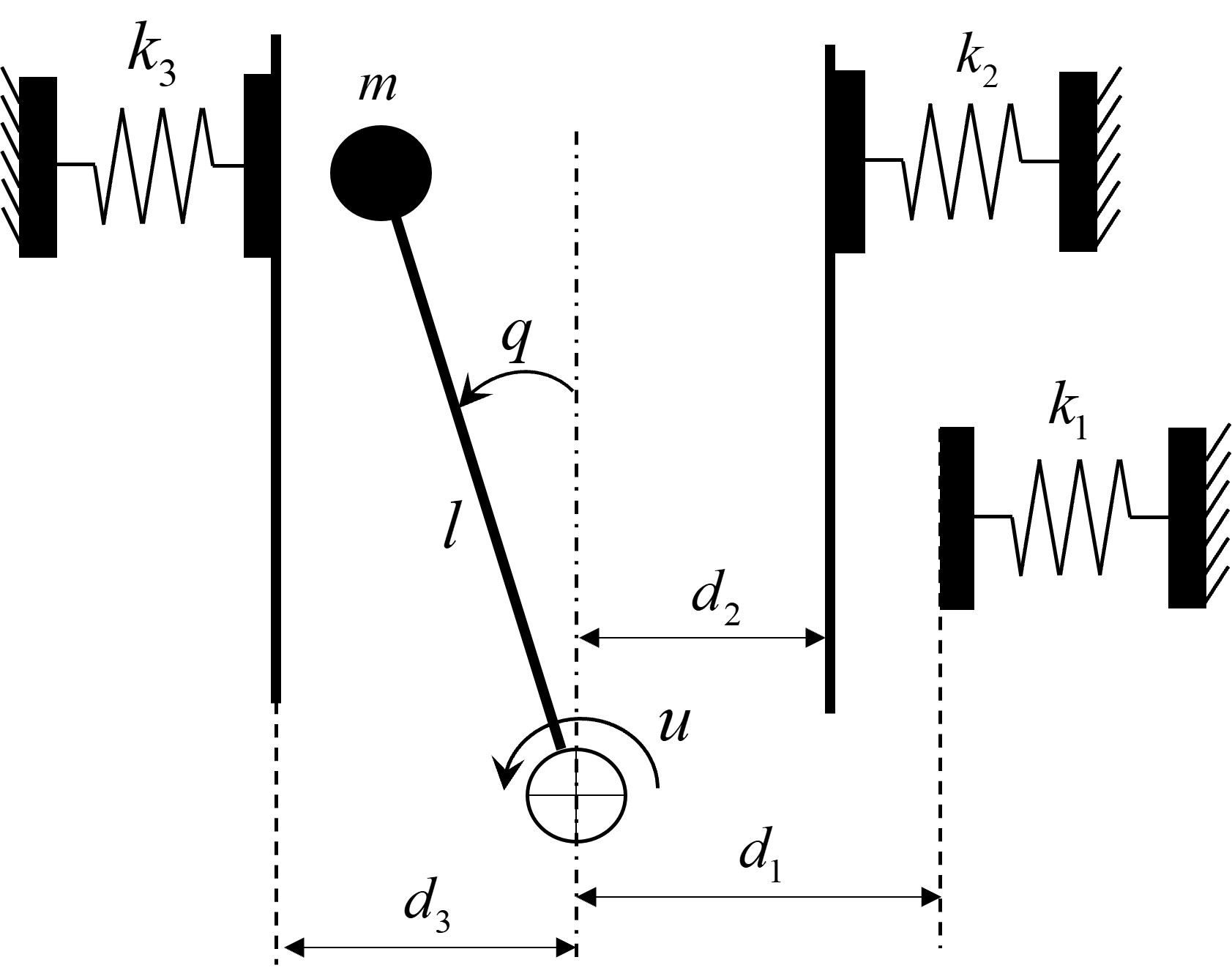
Model: Fig. 1 displays the inverted pendulum system. By linearizing the dynamics around the vertical configuration $\theta=\dot{\theta}=0$ and discretizing the system with a sampling time 0.05 s, we obtain a piecewise affine system:

$$x_{t+1}=A_{i}x_{t}+Bu_{t}+f_{i}\quad\text{ if }\;x_{t}\in\mathcal{C}_{i},\;i=1,2,3,4,$$

where the system matrices and the regions are given by

$$A_{1} =\left[\begin{array}[]{cc}1&0.05\\ -29.5&1\end{array}\right],\quad B=\left[\begin{array}[]{c}0\\ 0.05\end{array}\right],\quad f_{1}=\left[\begin{array}[]{l}0\\ -3.3\end{array}\right],\quad\mathcal{C}_{1}=\{(x,u)\mid[1\;\;0]x\leq-0.12\},$$

$$A_{2} =\left[\begin{array}[]{cc}1&0.05\\ -14.5&1\end{array}\right],\quad f_{2}=\left[\begin{array}[]{l}0\\ -1.5\end{array}\right],\quad\mathcal{C}_{2}=\{(x,u)\mid-0.12\leq[1\;\;0]x\leq-0.1\},$$

$$A_{3} =\left[\begin{array}[]{cc}1&0.05\\ 0.5&1\end{array}\right],\quad f_{3}=\left[\begin{array}[]{l}0\\ 0\end{array}\right],\quad\mathcal{C}_{3}=\{(x,u)\mid-0.1\leq[1\;\;0]x\leq 0.1\},$$

$$A_{4} =\left[\begin{array}[]{cc}1&0.05\\ -24.5&1\end{array}\right],\quad f_{4}=\left[\begin{array}[]{l}0\\ 2.5\end{array}\right],\quad\mathcal{C}_{4}=\{(x,u)\mid[1\;\;0]x\geq 0.1\}.$$

Controllers: We use four different controllers in the simulation.

(i) MPC: We take the horizon $N=5$, 6, or 7. For the stage cost $C_{\mathrm{MPC}}:\mathcal{X}\times\mathcal{U}\to\mathbb{R}_{\geq 0}$, we let $C(x,u)=x^{T}Qx+Ru^{2}$ with $Q=\mathrm{diag}([20\;\;1])$ and $R=1$. The terminal stage cost is $x^{T}_{N}Q_{\mathrm{T}}x_{N}$ with $Q_{\mathrm{T}}$ obtained by solving the discrete algebraic Riccati equation for the subsystem $x_{t+1}=A_{3}x_{t}+Bu_{t}$ whose region contains the origin. The terminal constraint set is the maximal positively invariant set for the autonomous system $x_{t+1}=(A_{3}-BK)x_{t}$ with $K$ the solution to the above-mentioned discrete algebraic Riccati equation. Owning to the quadratic nature of the cost function and the PWA property of the predictive model, the MPC problem can be equivalently converted into a mixed-integer convex quadratic programming problem [34], and consequently, globally optimal solutions can be found efficiently by using the branch-and-bound approach [24]. We use Gurobi [31] to solve the MPC problem online.

(ii) Supervised learning MPC: Following the approach in [19], we use an explicit controller, more precisely, an NN with three hidden ReLU layers containing 16, 32, and 8 neurons, to approximate the implicit MPC control law $u_{\mathrm{MPC}}$. In particular, we uniformly randomly sample the states from the state constraint set and select 4000 states that make the above-mentioned MPC problem with $N=7$ feasible. Next, 4000 state-input pairs $\{x_{i},\;u_{\mathrm{MPC}}(x_{i})\}_{i=1}^{4000}$ are obtained by solving the MPC problems with different initial conditions, and the NN is trained on these data pairs to approximate the map $u_{\mathrm{MPC}}$.

(iii) Approximate dynamic programming: As demonstrated in [3], ADP can produce a safe control policy by adding penalty terms in the cost function. In the ADP scheme, the objective is to find a control policy $\pi:\mathcal{X}\to\mathcal{U}$ to minimize the infinite-horizon cost

$$J_{\pi}\left(x_{0}\right)=\sum_{t=0}^{\infty}C_{\mathrm{RL}}\left(x_{t},\pi\left(x_{t}\right)\right)$$ (28)

for any initial state $x_{0}\in\mathcal{X}$. Following the existing literature [3, 35], the state cost is specified as $C_{\mathrm{RL}}(x,u)=C_{\mathrm{MPC}}(x,u)+30\max\{0,|x_{1}|-0.15\}+3\max\{0,|x_{2}|-1\}$, where the second and third terms penalize the state constraint violation. The ADP algorithm uses a policy NN and a value NN, which evaluates $J_{\pi}$, to find the optimal policy iteratively, and terminates when the parameters of the value NN undergo sufficiently slight changes in two consecutive iterations. One can see Algorithm 2 in [3] for details. Although the training of the ADP policy accommodates state constraints, the ADP policy can still cause constraint violation because (i) the penalty terms in $C_{\mathrm{RL}}$ are external penalties and thus do not strictly guarantee constraint satisfaction, and (ii) there are approximation errors in the policy and value NNs. It can be observed from Table 1 that the proposed safe filters improve the safety of the ADP policy.

(iv) LQR: the LQR feedback control law $u_{\mathrm{LQR}}=-Kx$, which is obtained when computing MPC in (i), can also be applied as the basic policy $\pi_{0}$ in the safety filters (II-B) and (15). When testing $u_{\mathrm{LQR}}$ without any safety filters, we simply project the resulting input value onto the input constraint set, which is a convex quadratic program.

References

- [1] J. F. Fisac, A. K. Akametalu, M. N. Zeilinger, S. Kaynama, J. Gillula, and C. J. Tomlin, “A general safety framework for learning-based control in uncertain robotic systems,” IEEE Transactions on Automatic Control, vol. 64, no. 7, pp. 2737–2752, 2018.
- [2] B. Thananjeyan, A. Balakrishna, U. Rosolia, F. Li, R. McAllister, J. E. Gonzalez, S. Levine, F. Borrelli, and K. Goldberg, “Safety augmented value estimation from demonstrations (saved): Safe deep model-based RL for sparse cost robotic tasks,” IEEE Robotics and Automation Letters, vol. 5, no. 2, pp. 3612–3619, 2020.
- [3] K. He, S. Shi, T. v. d. Boom, and B. De Schutter, “Approximate dynamic programming for constrained piecewise affine systems with stability and safety guarantees,” arXiv preprint arXiv:2306.15723, 2023.
- [4] L. Zheng, Y. Shi, L. J. Ratliff, and B. Zhang, “Safe reinforcement learning of control-affine systems with vertex networks,” in Learning for Dynamics and Control. PMLR, 2021, pp. 336–347.
- [5] Y. Li, N. Li, H. E. Tseng, A. Girard, D. Filev, and I. Kolmanovsky, “Robust action governor for uncertain piecewise affine systems with non-convex constraints and safe reinforcement learning,” arXiv preprint arXiv:2207.08240, 2022.
- [6] S. Adhau, V. V. Naik, and S. Skogestad, “Constrained neural networks for approximate nonlinear model predictive control,” in 2021 60th IEEE Conference on Decision and Control (CDC), 2021, pp. 295–300.
- [7] C. Dawson, S. Gao, and C. Fan, “Safe control with learned certificates: A survey of neural Lyapunov, barrier, and contraction methods for robotics and control,” IEEE Transactions on Robotics, 2023.
- [8] A. D. Ames, X. Xu, J. W. Grizzle, and P. Tabuada, “Control barrier function based quadratic programs for safety critical systems,” IEEE Transactions on Automatic Control, vol. 62, no. 8, pp. 3861–3876, 2016.
- [9] M. Lazar, M. Heemels, S. Weiland, and A. Bemporad, “Stabilizing model predictive control of hybrid systems,” IEEE Transactions on Automatic Control, vol. 51, no. 11, pp. 1813–1818, 2006.
- [10] S. Prajna, A. Jadbabaie, and G. J. Pappas, “A framework for worst-case and stochastic safety verification using barrier certificates,” IEEE Transactions on Automatic Control, vol. 52, no. 8, pp. 1415–1428, 2007.
- [11] A. Robey, H. Hu, L. Lindemann, H. Zhang, D. V. Dimarogonas, S. Tu, and N. Matni, “Learning control barrier functions from expert demonstrations,” in 2020 59th IEEE Conference on Decision and Control (CDC), 2020, pp. 3717–3724.
- [12] H. Dai, B. Landry, M. Pavone, and R. Tedrake, “Counter-example guided synthesis of neural network Lyapunov functions for piecewise linear systems,” in 2020 59th IEEE Conference on Decision and Control, 2020, pp. 1274–1281.
- [13] J. J. Choi, D. Lee, K. Sreenath, C. J. Tomlin, and S. L. Herbert, “Robust control barrier–value functions for safety-critical control,” in 2021 60th IEEE Conference on Decision and Control (CDC), 2021, pp. 6814–6821.
- [14] A. Didier, R. C. Jacobs, J. Sieber, K. P. Wabersich, and M. N. Zeilinger, “Approximate predictive control barrier functions using neural networks: A computationally cheap and permissive safety filter,” in 2023 European Control Conference (ECC), 2023, pp. 1–7.
- [15] K. P. Wabersich and M. N. Zeilinger, “Predictive control barrier functions: Enhanced safety mechanisms for learning-based control,” IEEE Transactions on Automatic Control, vol. 68, no. 5, pp. 2638–2651, 2023.
- [16] M. Korda, “Computing controlled invariant sets from data using convex optimization,” SIAM Journal on Control and Optimization, vol. 58, no. 5, pp. 2871–2899, 2020.
- [17] K. P. Wabersich, A. J. Taylor, J. J. Choi, K. Sreenath, C. J. Tomlin, A. D. Ames, and M. N. Zeilinger, “Data-driven safety filters: Hamilton-Jacobi reachability, control barrier functions, and predictive methods for uncertain systems,” IEEE Control Systems Magazine, vol. 43, no. 5, pp. 137–177, 2023.
- [18] A. Agrawal and K. Sreenath, “Discrete control barrier functions for safety-critical control of discrete systems with application to bipedal robot navigation.” in Robotics: Science and Systems, vol. 13. Cambridge, MA, USA, 2017, pp. 1–10.
- [19] B. Karg and S. Lucia, “Efficient representation and approximation of model predictive control laws via deep learning,” IEEE Transactions on Cybernetics, vol. 50, no. 9, pp. 3866–3878, 2020.
- [20] D. P. Bertsekas, Reinforcement Learning and Optimal Control. Athena Scientific, 2019.
- [21] A. Alessio, M. Lazar, A. Bemporad, and M. Heemels, “Squaring the circle: An algorithm for generating polyhedral invariant sets from ellipsoidal ones,” Automatica, vol. 43, no. 12, pp. 2096–2103, 2007.
- [22] A. Mesbah, K. P. Wabersich, A. P. Schoellig, M. N. Zeilinger, S. Lucia, T. A. Badgwell, and J. A. Paulson, “Fusion of machine learning and MPC under uncertainty: What advances are on the horizon?” in 2022 American Control Conference (ACC), 2022, pp. 342–357.
- [23] A. Rinnooy Kan and G. Timmer, “Stochastic global optimization methods part ii: Multi level methods,” Mathematical Programming, vol. 39, pp. 57–78, 1987.
- [24] L. A. Wolsey and G. L. Nemhauser, Integer and Combinatorial Optimization. John Wiley & Sons, 1999, vol. 55.
- [25] M. Hertneck, J. Köhler, S. Trimpe, and F. Allgöwer, “Learning an approximate model predictive controller with guarantees,” IEEE Control Systems Letters, vol. 2, no. 3, pp. 543–548, 2018.
- [26] F. Moreno-Mora, L. Beckenbach, and S. Streif, “Predictive control with learning-based terminal costs using approximate value iteration,” arXiv preprint arXiv:2212.00361, 2022.
- [27] K. He, T. v. d. Boom, and B. De Schutter, “Approximate dynamic programming for constrained linear systems: A piecewise quadratic approximation approach,” arXiv preprint arXiv:2205.10065, 2022.
- [28] B. Hanin, “Universal function approximation by deep neural nets with bounded width and ReLU activations,” Mathematics, vol. 7, no. 10, p. 992, 2019.
- [29] L. Busoniu, R. Babuska, B. De Schutter, and D. Ernst, Reinforcement Learning and Dynamic Programming Using Function Approximators. CRC Press, 2017.
- [30] J. F. Fisac, N. F. Lugovoy, V. Rubies-Royo, S. Ghosh, and C. J. Tomlin, “Bridging Hamilton-Jacobi safety analysis and reinforcement learning,” in 2019 International Conference on Robotics and Automation (ICRA). IEEE, 2019, pp. 8550–8556.
- [31] L. Gurobi Optimization, “Gurobi optimizer reference manual,” 2021.
- [32] I. Goodfellow, Y. Bengio, and A. Courville, Deep Learning. MIT Press, 2016.
- [33] J. B. Rawlings, D. Q. Mayne, and M. Diehl, Model Predictive Control: Theory, Computation, and Design. Nob Hill Publishing Madison, WI, 2017, vol. 2.
- [34] F. Borrelli, A. Bemporad, and M. Morari, Predictive Control for Linear and Hybrid Systems. Cambridge University Press, 2017.
- [35] P. N. Beuchat and J. Lygeros, “Approximate dynamic programming via penalty functions,” IFAC-PapersOnLine, vol. 50, no. 1, pp. 11 814–11 821, 2017.