Evaluation of Barlow Twins and VICReg self-supervised learning for sound patterns of bird and anuran species

Abstract

Taking advantage of the structure of large datasets to pre-train Deep Learning models is a promising strategy to decrease the need for supervised data. Self-supervised learning methods, such as contrastive and its variation are a promising way towards obtaining better representations in many Deep Learning applications. Soundscape ecology is one application in which annotations are expensive and scarce, therefore deserving investigation to approximate methods that do not require annotations to those that rely on supervision. Our study involves the use of the methods Barlow Twins and VICReg to pre-train different models with the same small dataset with sound patterns of bird and anuran species. In a downstream task to classify those animal species, the models obtained results close to supervised ones, pre-trained in large generic datasets, and fine-tuned with the same task.

Keywords sound event identification, animal species classification, classification improvement

1 Introduction

Sound is an important attribute to understanding landscape dynamics Pijanowski et al. (2011) and represents a relevant feature when investigating Machine Learning Kong et al. (2020) in the context of soundscape ecology. In that sense, recent research has focused on defining well-suited approaches to deal with natural sound tasks Dufourq et al. (2022); Stowell (2022). Those strategies are concentrated on Convolutional Neural Networks (CNNs) because they can recognize temporal-frequency patterns Salamon and Bello (2017) and obtain proper results in many sound-related tasks Kahl et al. (2021); LeBien et al. (2020).

However, CNNs are data-hungry and the acquisition of large and accurately labeled datasets is difficult and time-consuming requiring alternative training strategies Ponti et al. (2021). To handle this issue, Deep Learning specialists and researchers are attempting to take advantage of a large amount of unlabeled data available throughout the Internet with Self-supervised learning (SSL) de Sa (1994). For example, Baevski et al. (2020) developed a process capable of learning both contextualized speech representation and discretized speech units; and  Saeed et al. (2021) created a framework to learn general-purpose representations of speech sounds.

In this paper, we conducted experiments with contrastive methods, a popular SSL approach that minimizes the distance between similar patterns while maximizing the distance between unrelated patterns Saeed et al. (2021). Instead of using large unlabeled datasets, such as the aforementioned examples, we mainly evaluated the behavior of these techniques in cases in which the pre-training dataset has the same samples as the downstream task but with different views. Even in such a restricted pre-training scenario, SSL techniques pre-trained models that reached results near to models pre-trained on well-known supervised tasks with large datasets. The best models and codes will be available on GitHub.

The subsequent sections are constructed as follows. section 2 concisely reviews the SSL approaches tested in this research. section 3 presents the steps followed and the materials used in our experiments. section 4 reports the experimental results obtained with the experiments. section 5 discusses the experimental results. Finally, section 6 provides the conclusions and directions for future work.

2 Technical Background

With SSL strategies, it is possible to use auxiliary tasks, whose labels are created from the dataset structure, and the learned weights are transferred to specific tasks, obtaining suitable results in many real applications Baevski et al. (2020); Chi et al. (2021); Owens and Efros (2018).

One recurrent SSL technique pre-trains a model with branches that learn similar invariant embeddings of different data views Bardes et al. (2022). As an example, Barlow Twins Zbontar et al. (2021) has a structure with two consecutive blocks, an encoder and a projector. The former can be any CNN without the classification layer and the latter has three dense layers with $N$ units, batch normalization before ReLU activation (two first layers), and the last layer only with linear activation. Barlow Twins authors claim that the projector removes space redundancy of the encoder. This two-block structure configures each branch of a Siamese network Bromley et al. (1994); Chopra et al. (2005) with shared weights between the branches. Such a method shows good representation learning ability while maintaining robustness to attack scenarios Cavallari and Ponti (2022). The architecture receives two different views of the input and forces their embeddings to be close, minimizing component redundancy of the learned features by employing the following contrastive loss function:

$$L_{BT}=\underbrace{\sum_{i}(1-C_{ii})^{2}}_{\text{invariance term}}+\underbrace{\lambda\sum_{i}\sum_{i\neq j}C_{ij}^{2}}_{\text{redundancy reduction term}}\text{,}$$ (1)

being $\lambda$ a hyperparameter that controls the term importance and $C$ the cross-correlation matrix of the spaces of the network branches. The invariance term forces the encoder spaces to be close and the second term reduces the spaces’ redundancy. Besides, it can avoid space collapse to constant values or irrelevant data information. After the training, the encoder is extracted and fine-tuned in a downstream task.

As a variation of this idea, Bardes et al. (2022) also defined the Variance-Invariance-Covariance Regularization (VICReg) to avoid space collapse. This regularization technique can stabilize the training process, leading to results close to the state-of-the-art in many downstream tasks. We can use it with the Barlow Twins configuration but with the following contrastive loss function:

$$\begin{split}\ell(Z_{a},Z_{b})&=\underbrace{\lambda\frac{1}{n}\sum mse(Z_{a},Z_{b})}_{\text{invariance}}+\underbrace{\mu\left[v(Z_{a})+v(Z_{b})\right]}_{\text{variance}}+\underbrace{\nu\left[c(Z_{a})+c(Z_{b})\right]}_{\text{covariance}}\text{,}\end{split}$$

being $Z_{i}$ a data batch with $n$ vectors learned by the expander (projector) of each network branch, and $\lambda$, $\mu$, and $\nu$ hyperparameters. The invariance term is the mean squared error (mse) between the spaces, and the variance and covariance are defined as:

$$v(Z)=\frac{1}{n}\sum relu(\gamma-\sqrt{var(Z)+\epsilon})\text{,}$$

$$c(Z)=\frac{1}{N}\sum_{i}\sum_{i\neq j}C(Z)_{ij}^{2}\text{,}$$

$$C(Z)=\frac{\left\lVert Z-mean(Z)\right\rVert_{2}}{N-1}\text{,}$$

where $N$ is the space size of the expander, $\gamma=1$, $\epsilon=10^{-4}$, and $mean$ and $var$ are calculated for the batch. The invariance term has the same purpose as in the Barlow Twins, the variance term does not allow the vectors to point to the same place, and the covariance term reduces the redundancy of the learned vectors.

3 Method

This section presents the steps to evaluate SSL strategies to pre-train CNNs used to identify animal species. In the first step, the training subset of Table 1 was balanced by data augmentation strategies for sound signals. We used these same techniques to create different views to feed the SSL tasks. During the second step, we built a baseline by fine-tuning models to identify sound patterns with weights randomly initialized or pre-trained on generic image classification tasks. The third step consists of pre-training models with SSL tasks and fine-tuning them to also identify sound patterns.

3.1 Dataset

Our dataset in Table 1 contains recordings collected on natural landscapes, provided by the Spatial Ecology and Conservation Lab (LEEC) , and already explored by Scarpelli et al. (2021); Hilasaca et al. (2021a, b); Dias et al. (2021). These data are part of the Long Term Ecological Research conducted at the Cantareira-Mantiqueira ecological corridor (LTER CCM), which is localized in the northeast portion of Sao Paulo state, Brazil. Moreover, following Kahl et al. (2021), the table has samples from Google AudioSet Gemmeke et al. (2017), forming a dataset with 15 classes. To download AudioSet recordings, we employed youtube-dl (v2021.4.26) library.

The dataset was split using a stratified method of the classes in training (90%) and test (10%), totaling 5000 clips of 3 seconds (250 min. in total), as showed in Table 1. We applied $k$-fold cross-validation with $k=5$ in the training subset and for each iteration, one partition was used as a validation subset. In that sense, fine-tuning tasks used training, validation, and test subsets, meanwhile, SSL auxiliary tasks used only the training and validation subsets.

Table 1: Quantities of 3-second audio clips grouped by species and named with a short label

	specie	label	#train	#test	Total
bird	Basileuterus culicivorus	basi_culi	483	54	537
	Cyclarhis gujanensis	cycl_guja	390	43	433
	Myiothlypis leucoblephara	myio_leuc	411	46	457
	Pitangus sulphuratus	pita_sulp	352	39	391
	Vireo chivi	vire_chiv	724	81	805
	Zonotrichia capensis	zono_cape	574	64	638
			2934	327	3261
anuran	Adenomera marmorata	aden_marm	116	13	129
	Aplastodiscus leucopigyus	apla_leuc	186	21	207
	Boana albopunctata	boan_albo	283	32	315
	Dendropsophus minutus	dend_minu	229	26	255
	Ischnocnema guenteri	isch_guen	136	15	151
	Physalaemus cuvieri	phys_cuvi	290	32	322
			1240	139	1379
other		animal	108	12	120
		human	109	11	120
		natural	109	11	120
			326	34	360
Total			4500	500	5000

3.2 Balancing data classes

The dataset was augmented both to reduce possible problems, such as model poor generalization and improper predictions for samples of minority classes Johnson and Khoshgoftaar (2019); Wang et al. (2017), and to create different data views for SSL tasks.

To fine-tune model weights, augmentation generated $m=\lceil(\max_{c}-\#class)/\#class\rceil$ modified copies of all 3-second training recordings that were added to the original training subset to generate spectrograms. When cross-validation split training files, we first divide the originals into 3600 files ($k-1$ partitions) for training and 900 samples for validation. After that, we take augmentations until each class in the training subset reaches $\max_{c}=580$ audio clips, generating a set with 8700 clips. The choice of 580 is to approach the majority class (Vireo chivi) in the training subset. Hence, in each cross-validation iteration, there are 8700 clips for training, 900 clips for validation, and 500 clips for testing.

We considered time stretching, pitch shifting, and noise addition as proposed by Salamon and Bello (2017), following the same implementations used in Dias et al. (2021) and parameters of Table 2.

Table 2: Values range for the augmentation parameters.

	values
stretch (factor)	from 0.7 to 1.3, incremented by 0.1 (discards 0.0)
pitch (steps)	$[-12,-6,-3,3,6,12]$
noise (dB)	from 2 to 12, incremented by 2

For SSL tasks, augmentation creates two alternative views for each training and validation subset sample. The process randomly chooses two functions and their respective parameters described in Table 2. After cross-validation splits data in training and validation, equal to the past description, the augmentation generates alternative views and each iteration has 7200 samples for training and 1800 for validation.

3.3 Audio spectrograms

For all audio clips, gray-scale mel-spectrogram images (256$\times$256) were created with librosa (v0.8.1) routines, using a Hanning window with a length of 2048 and an overlap of 75%. Length and overlap contribute to building a representation with suitable frequency and time resolutions to represent a large pattern variation.

3.4 Network architectures

We employed four network architectures: one proposed by Salamon and Bello (2017), named here as SimpleCNN, MobileNet-V3 (Large) Howard et al. (2019), ResNet-50 He et al. (2016), and Inception-V3 Szegedy et al. (2016), all of them pre-trained on ImageNet Deng et al. (2009) when necessary. SimpleCNN achieved suitable results to classify bird species, MobileNet is an architecture built to consume less computational resources, ResNet is a common option to classify animal species Harvey (2018); LeBien et al. (2020); Thomas et al. (2019), and Inception has filter variations that could improve the learning process of patterns with different sizes.

To train SimpleCNN and MobileNet-V3, we used SGD optimizer with learning rate $lr=10^{-2}$ and $momentum=0.9$ (only MobileNet-V3). ResNet-50 used Adam with $lr=10^{-4}$ and Inception-V3 used RMSProp with $lr=10^{-3}$. All training processes executed 100 epochs with $batch=80$, except ResNet-50, whose $batch=30$.

SSL tasks and fine-tuning used the same configurations, changing the batch size because of memory constraints: 30 samples for ResNet-50 and 50 samples for the others. All inputs were normalized with max-norm, dividing pixels values by 255.

We created a SimpleCNN version pre-trained on a small version of ImageNet. We used $\approx 28\%$ (358.727 samples) from the training subset and maintained the samples of validation (50K samples) and test (100K samples). This pre-training considered the same optimization setup described in the preceding paragraphs with $batch=256$.

Models were implemented with Python (v3.8.10) associated with TensorFlow/Keras (v2.7.0) library.

3.5 Self-supervised tasks

We considered the Barlow Twins and VICReg described in section 2. Their inputs are mel-spectrograms of the views generated by the section 3.2 and the models are initialized with random weights. The configuration of the respective loss functions follow the hyperparameters defined in the original papers: Barlow Twins $\lambda=0.005$; and VICReg $\lambda=\mu=25$, $\nu=\gamma=1$, and $\epsilon=10^{-4}$.

The encoder of both tasks are configured with one of the cited architectures, discarding the SimpleCNN dense layers, and replacing the top layers of the other networks with global average pooling. Furthermore, the three dense layers of the projector have $N=512$.

After pre-training, we extracted the encoder of the task that achieved the best loss function value in the validation subset. Besides, we added the top layers of each model (randomly initialized) and fine-tuned the learned weights.

3.6 Evaluation

We evaluated the results with the balanced accuracy score of scikit-learn (v1.0.1) Pedregosa et al. (2011). We also employed a two-tailed Student’s t-test to compare results using paired tests with a significance level equal to 0.05.

In all tests, we used Python seed values (1030), following the Keras FAQ. As aforesaid, we used cross-validation with $k=5$ in both cases pre-train and fine-tune. For SSL pre-training, we evaluated the loss function in the validation subset, and for fine-tuning we considered the mean and standard deviation of the balanced accuracy of the test subset.

To perform comparisons, we executed three cases: in the first, all weights were randomly initialized; in the second, with weights learned on ImageNet; and finally, with weights learned with SSL tasks. We fine-tuned models to classify 15 classes, but we assessed them with twelve classes related to the specific animal species of interest (see Table 1), to facilitate comparisons with previous works.

Besides, we evaluated the impact of changing the number of samples: i) doubling the training subset with more unlabeled samples from LEEC data to pre-train with SSL tasks, ii) and diminishing the training subset to fine-tune the models to 50% and 20% of the training subset in Table 1. We also assessed variations of the projector space size $N\in[512,1024,2048,4096,8192]$ to compare with the results of Zbontar et al. (2021); Bardes et al. (2022). We tested only with the best combination of model and SSL task (ResNet50 and VICReg) and used the same configurations of section 3.4 to pre-train the model, with $batch=90$ (smallest $N$), $batch=80$ (largest $N$).

Associated with balanced accuracy, we employed silhouette coefficient Tan et al. (2005) to numerically evaluate learned features and t-SNE Maaten and Hinton (2008) that visually helps the evaluation of classes’ neighborhoods and their segregation Nonato and Aupetit (2018). To perform this, we extracted features from the penultimate layer because they are the inputs for the classification layer. The routines to generate silhouettes and projections are also available on scikit-learn.

Finally, the majority of training and tests were performed with an NVidia Titan XP video card, with driver v470.86, Cuda v11.2.152, and cuDNN v8.1.0. The SimpleCNN pre-train on ImageNet and the variation of projector space were executed with an NVidia RTX A5000 video card, with driver v470.74, Cuda v11.4, and cuDNN v8.1.0.

4 Results

This section reports the results of our experiments with SSL tasks. Such results were compared with those of the same models initialized with random weights and weights learned on ImageNet. The evaluation uses balanced accuracy $\in[0,1]$, silhouette coefficient $\in[-1,1]$, and t-SNE projections. We executed two SSL tasks: Barlow Twins and VICReg; four CNNs, named: SimpleCNN, MobileNetV3, ResNet50, and InceptionV3, all fed with mel-spectrogram images. Finally, tests were executed with $5$-fold cross-validation.

Table 3: Results of models randomly initialized, pre-trained on ImagetNet, and SSL tasks. Both silhouette coefficient and balanced accuracy were calculated for the test subset. Silhouette is related to the best cross-validation partition. Highlighted values are the best results.

	Random		ImageNet
	silhouette	balan.acc.	silhouette	balan.acc.
SimpleCNN	0.0065	0.60$\pm$ 0.02	0.0340	0.61$\pm$ 0.02
MobileNetV3	0.0863	0.62$\pm$ 0.03	0.1500	0.70$\pm$ 0.01
ResNet50	0.0769	0.65$\pm$ 0.03	0.2240	0.77$\pm$ 0.01
InceptionV3	0.1150	0.67$\pm$ 0.03	0.1303	0.77$\pm$ 0.02
	Barlow Twins		VICReg
SimpleCNN	-0.0031	0.55$\pm$ 0.02	0.0142	0.61$\pm$ 0.01
MobileNetV3	-0.1213	0.23$\pm$ 0.07	0.0085	0.54$\pm$ 0.03
ResNet50	0.1041	0.69$\pm$ 0.03	0.1374	0.72$\pm$ 0.02
InceptionV3	0.0451	0.68$\pm$ 0.02	0.0109	0.68$\pm$ 0.02

Table 3 and Figure 1 summarize the results. In all test cases, ResNet50 and InceptionV3 obtain similar results (do not reject the null hypothesis with p-value $>0.05$) and are always superior to the other models, with more than 3 percent points of difference. ResNet50 also reached the highest silhouette coefficient in all pre-trained cases.

Random initialization and transfer from ImageNet are respectively lower and higher bounds of the results and the two SSL strategies reduced silhouette ($<0.14$) and balanced accuracy ($\leq 0.72$) results when compared with the higher bounds (silhouette $<0.23$ and accuracy $\leq 0.77$). In that sense, MobileNet suffered the most with SSL pre-training, reducing the results to values below the random initialization. The comparisons between Barlow Twins and VICReg show that the latter has results at least 3 percent points greater than the former SSL, except for InceptionV3. These and other differences and similarities between the results are more visible when analyzing Figure 1.

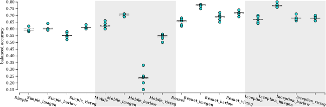
Figure 1: Individual value plots of balanced accuracy of CNNs applied to test subset. Each plot area (white and shade gray) shows the best results of a model with different weight initialization (from left to right: random, pre-trained on ImageNet, and pre-trained with SSL). Solid and dotted lines in each group communicate median and mean values, respectively. An overlap between points generates model results with a different number of points.

4.1 Learned feature space

Figure 2 has t-SNE projections to inspect the learned feature spaces visually. These images ratify the results described previously. Overall, the model’s depth impacts class segregation, being the features learned by SimpleCNN the ones that present more visual clutter, and ResNet50 and Inception the models that learned features with well-defined visual distinction. Furthermore, the models pre-trained with ImageNet achieve the best visual segregation. These behaviors reflect silhouette coefficients reported on Table 3. One can also verify that the innermost regions of the projections have more visual clutter than the outermost ones.

We also colored data points with two colors (bird and anuran), and it was possible to verify, independently of the model or weight initialization, a clear visual segregation between the two groups, even with some overlap level.

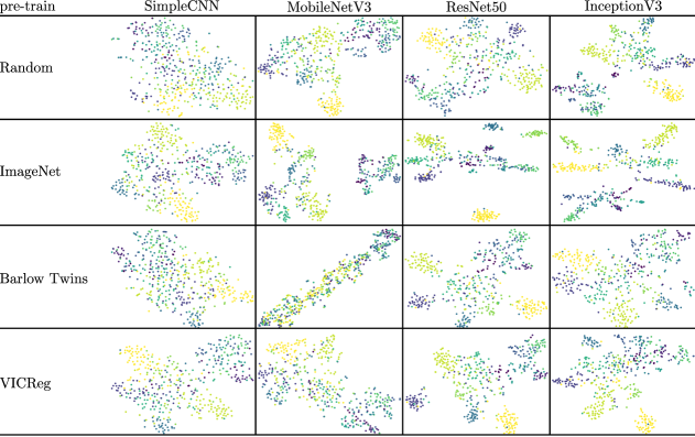
Figure 2: t-SNE projection of the test subset represented by model’s learned features. Each figure column shows the best results of a model with different weight initialization. Models were chosen from the best cross-validation partition of each test case. Point colors represent species of interest.

4.2 Variation of training samples

As we could expect when reducing the training subset to fine-tune the models, the balanced accuracy diminished significantly (reject the null hypothesis with p-value $\leq 0.05$). For example, ResNet50 pre-trained with VICReg: $0.72\pm 0.02$ (refined with 100% of training subset), $0.60\pm 0.02$ (refined with 50%), and $0.43\pm 0.02$ (refined with 20%).

Doubling the number of samples to execute SSL increased the processing time from one day to three days. This increment of samples impacts more Barlow Twins, increasing results in most cases. For example, it increased ResNet50 results from $0.69\pm 0.03$ (see Table 3) to $0.71\pm 0.01$, and MobileNetV3 from $0.23\pm 0.07$ to $0.32\pm 0.08$.

In both tests, following the Table 3, VICReg results are greater than or equal to Barlow Twins results.

4.3 Variation of self-supervision space

In this test, we considered only ResNet50 pre-trained with VICReg because it achieves the best SSL results on Table 3. The $N$ variations did not change significantly the results (not reject the null hypothesis with p-value $>0.05$). For example, with the smallest projector space ($N=512$) the fine-tuned ResNet50 obtains balanced accuracy of $0.70\pm 0.02$, while with the largest space ($N=8192$, best results on original papers) obtains $0.69\pm 0.02$.

5 Discussion

In general, random initialization of weights and weights transferred from ImagetNet tasks are lower bound (balanced accuracy mean $\in[0.60,0.67]$) and upper bound (balanced accuracy mean $\in[0.61,0.77]$) of the results. Hence, depending on the model used as encoder, models pre-trained with Barlow Twins achieved results close to random initialization, with maximum balanced accuracy equal to 0.69, while with VICReg, models achieved results up to 0.72. Such behavior is similar to the results reported by Bardes et al. (2022), which reports the superiority of VICReg results, highlighting its capability of producing more robust features. Furthermore, even with a small train (4500 samples from 15 classes), VICReg obtained models that can yield 5 percent points away from the ImageNet pre-trained models (+1M samples from 1K classes).

In our tests, independently of the weight initialization approach, the refined models have difficulties yielding balanced accuracy greater than 0.77 and silhouette coefficient greater than 0.23. This issue is related to the level of class overlap viewed in parts of Figure 2.

As could be expected, the fewer data samples for fine-tuning, the lesser the balanced accuracy of the models. However, models pre-trained with VICReg achieved the highest results than the ones pre-trained with Barlow Twins. Overall, adding more samples for pre-training did not significantly increase the results, except for MobileV3, which increased results from $0.23\pm 0.07$ to $0.32\pm 0.08$. Even so, it demands more tests to evaluate the impact of the size of the pre-train dataset on the final results. Besides, increasing pre-training samples also increased 3x the processing time.

Finally, variations of the projector space size did not impact the results and the balanced accuracy became stable at around 0.69. This behavior is different from the results of Zbontar et al. (2021); Bardes et al. (2022), which reported an improvement in the results when increasing the space size. Therefore we have to conduct more experiments to achieve a better understanding of it.

6 Conclusion

This paper reported a series of tests with SSL to evaluate their impact on CNNs fine-tuned to identify natural sound patterns. We have tested two SSL tasks and four architectures and compared the final results with the same models pre-trained on the ImageNet and initialized with random weights. In our tests, the VICReg strategy pre-trained models that converge to better results than Barlow Twins, following Bardes et al. (2022). Furthermore, even with a small train dataset (4500 samples from 15 classes), it is possible to pre-train with VICReg and fine-tune models that achieve balanced accuracy up to 0.72, while the same models pre-trained with ImageNet (+1M samples from 1K classes) reach 0.77.

Changes on the SSL hyperparameter (space size) did not corroborate with their original papers and increments of the dataset for pre-training did not generate significant improvements but increased the processing time 3x. Future work is necessary to understand variations of the dataset size, technique hyperparameter, and the applicability of other approaches, such as Cramer et al. (2019); Guzhov et al. (2022).

References

- Pijanowski et al. [2011] Bryan C. Pijanowski, Almo Farina, Stuart H. Gage, Sarah L. Dumyahn, and Bernie L. Krause. What is soundscape ecology? An introduction and overview of an emerging new science. Landscape Ecology, 26(9):1213–1232, 2011.
- Kong et al. [2020] Qiuqiang Kong, Yin Cao, Turab Iqbal, Yuxuan Wang, Wenwu Wang, and Mark D Plumbley. PANNs: Large-scale pretrained audio neural networks for audio pattern recognition. IEEE/ACM Transactions on Audio, Speech, and Language Processing, 28:2880–2894, 2020.
- Dufourq et al. [2022] Emmanuel Dufourq, Carly Batist, Ruben Foquet, and Ian Durbach. Passive acoustic monitoring of animal populations with transfer learning. Ecological Informatics, 70:101688, 2022.
- Stowell [2022] Dan Stowell. Computational bioacoustics with deep learning: a review and roadmap. PeerJ, 10:e13152, 2022.
- Salamon and Bello [2017] Justin Salamon and Juan Pablo Bello. Deep convolutional neural networks and data augmentation for environmental sound classification. IEEE Signal Processing Letters, 24(3):279–283, 2017.
- Kahl et al. [2021] Stefan Kahl, Connor M Wood, Maximilian Eibl, and Holger Klinck. BirdNET: A deep learning solution for avian diversity monitoring. Ecological Informatics, 61:101236, 2021.
- LeBien et al. [2020] Jack LeBien, Ming Zhong, Marconi Campos-Cerqueira, Julian P Velev, Rahul Dodhia, Juan Lavista Ferres, and T Mitchell Aide. A pipeline for identification of bird and frog species in tropical soundscape recordings using a convolutional neural network. Ecological Informatics, page 101113, 2020.
- Ponti et al. [2021] Moacir A Ponti, Fernando P dos Santos, Leo SF Ribeiro, and Gabriel B Cavallari. Training deep networks from zero to hero: avoiding pitfalls and going beyond. In 2021 34th SIBGRAPI Conference on Graphics, Patterns and Images (SIBGRAPI), pages 9–16. IEEE, 2021.
- de Sa [1994] Virginia R de Sa. Learning classification with unlabeled data. Advances in neural information processing systems, pages 112–112, 1994.
- Baevski et al. [2020] Alexei Baevski, Yuhao Zhou, Abdelrahman Mohamed, and Michael Auli. wav2vec 2.0: A framework for self-supervised learning of speech representations. Advances in Neural Information Processing Systems, 33:12449–12460, 2020.
- Saeed et al. [2021] Aaqib Saeed, David Grangier, and Neil Zeghidour. Contrastive learning of general-purpose audio representations. In ICASSP 2021 - 2021 IEEE International Conference on Acoustics, Speech and Signal Processing (ICASSP), pages 3875–3879, 2021.
- Chi et al. [2021] Po-Han Chi, Pei-Hung Chung, Tsung-Han Wu, Chun-Cheng Hsieh, Yen-Hao Chen, Shang-Wen Li, and Hung-yi Lee. Audio Albert: A Lite Bert for Self-Supervised Learning of Audio Representation. In 2021 IEEE Spoken Language Technology Workshop (SLT), pages 344–350. IEEE, 2021.
- Owens and Efros [2018] Andrew Owens and Alexei A Efros. Audio-visual scene analysis with self-supervised multisensory features. In Proceedings of the European Conference on Computer Vision (ECCV), pages 631–648, 2018.
- Bardes et al. [2022] Adrien Bardes, Jean Ponce, and Yann Lecun. VICReg: Variance-Invariance-Covariance regularization for Self-supervised learning. In ICLR 2022-10th International Conference on Learning Representations, 2022.
- Zbontar et al. [2021] Jure Zbontar, Li Jing, Ishan Misra, Yann LeCun, and Stéphane Deny. Barlow twins: Self-supervised learning via redundancy reduction. In International Conference on Machine Learning, pages 12310–12320. PMLR, 2021.
- Bromley et al. [1994] Jane Bromley, Isabelle Guyon, Yann LeCun, Eduard Säckinger, and Roopak Shah. Signature verification using a "siamese" time delay neural network. Advances in neural information processing systems, 6, 1994.
- Chopra et al. [2005] Sumit Chopra, Raia Hadsell, and Yann LeCun. Learning a similarity metric discriminatively, with application to face verification. In 2005 IEEE Computer Society Conference on Computer Vision and Pattern Recognition (CVPR’05), volume 1, pages 539–546. IEEE, 2005.
- Cavallari and Ponti [2022] Gabriel Biscaro Cavallari and Moacir A Ponti. Training strategies with unlabeled and few labeled examples under 1-pixel attack by combining supervised and self-supervised learning. In First Workshop on Pre-training: Perspectives, Pitfalls, and Paths Forward at ICML 2022, 2022.
- Scarpelli et al. [2021] Marina DA Scarpelli, Milton Cezar Ribeiro, and Camila P Teixeira. What does Atlantic Forest soundscapes can tell us about landscape? Ecological Indicators, 121:107050, 2021.
- Hilasaca et al. [2021a] Liz Maribel Huancapaza Hilasaca, Lucas Pacciullio Gaspar, Milton Cezar Ribeiro, and Rosane Minghim. Visualization and categorization of ecological acoustic events based on discriminant features. Ecological Indicators, 126:107316, 2021a.
- Hilasaca et al. [2021b] Liz Huancapaza Hilasaca, Milton Cezar Ribeiro, and Rosane Minghim. Visual Active Learning for labeling: A case for Soundscape Ecology data. Information, 12(7):265, 2021b.
- Dias et al. [2021] Fábio Felix Dias, Moacir Antonelli Ponti, and Rosane Minghim. A classification and quantification approach to generate features in soundscape ecology using neural networks. Neural Computing and Applications, 34(3):1923–1937, sep 2021.
- Gemmeke et al. [2017] Jort F. Gemmeke, Daniel P. W. Ellis, Dylan Freedman, Aren Jansen, Wade Lawrence, R. Channing Moore, Manoj Plakal, and Marvin Ritter. Audio set: An ontology and human-labeled dataset for audio events. In Proc. IEEE ICASSP 2017, New Orleans, LA, 2017.
- Johnson and Khoshgoftaar [2019] Justin M Johnson and Taghi M Khoshgoftaar. Survey on deep learning with class imbalance. Journal of Big Data, 6(1):1–54, 2019.
- Wang et al. [2017] Jason Wang, Luis Perez, et al. The effectiveness of data augmentation in image classification using deep learning. Convolutional Neural Networks Vis. Recognit, 11:1–8, 2017.
- Howard et al. [2019] Andrew Howard, Mark Sandler, Grace Chu, Liang-Chieh Chen, Bo Chen, Mingxing Tan, Weijun Wang, Yukun Zhu, Ruoming Pang, Vijay Vasudevan, et al. Searching for mobilenetv3. In Proceedings of the IEEE/CVF International Conference on Computer Vision, pages 1314–1324, 2019.
- He et al. [2016] Kaiming He, Xiangyu Zhang, Shaoqing Ren, and Jian Sun. Deep residual learning for image recognition. In Proceedings of the IEEE conference on computer vision and pattern recognition, pages 770–778, 2016.
- Szegedy et al. [2016] Christian Szegedy, Vincent Vanhoucke, Sergey Ioffe, Jon Shlens, and Zbigniew Wojna. Rethinking the inception architecture for computer vision. In Proceedings of the IEEE conference on computer vision and pattern recognition, pages 2818–2826, 2016.
- Deng et al. [2009] Jia Deng, Wei Dong, Richard Socher, Li-Jia Li, Kai Li, and Li Fei-Fei. Imagenet: A large-scale hierarchical image database. In 2009 IEEE conference on computer vision and pattern recognition, pages 248–255. Ieee, 2009.
- Harvey [2018] Matt Harvey. Acoustic Detection of Humpback Whales Using a Convolutional Neural Network, 10 2018. URL https://ai.googleblog.com/2018/10/acoustic-detection-of-humpback-whales.html.
- Thomas et al. [2019] Mark Thomas, Bruce Martin, Katie Kowarski, Briand Gaudet, and Stan Matwin. Marine mammal species classification using convolutional neural networks and a novel acoustic representation. In Joint European Conference on Machine Learning and Knowledge Discovery in Databases, pages 290–305. Springer, 2019.
- Pedregosa et al. [2011] F. Pedregosa, G. Varoquaux, A. Gramfort, V. Michel, B. Thirion, O. Grisel, M. Blondel, P. Prettenhofer, R. Weiss, V. Dubourg, J. Vanderplas, A. Passos, D. Cournapeau, M. Brucher, M. Perrot, and E. Duchesnay. Scikit-learn: Machine learning in Python. Journal of Machine Learning Research, 12:2825–2830, 2011.
- Tan et al. [2005] Pang-Ning Tan, Michael Steinbach, and Vipin Kumar. Introduction to data mining. 1st, 2005.
- Maaten and Hinton [2008] Laurens van der Maaten and Geoffrey Hinton. Visualizing data using t-SNE. Journal of Machine Learning Research, 9(Nov):2579–2605, 2008.
- Nonato and Aupetit [2018] Luis Gustavo Nonato and Michael Aupetit. Multidimensional projection for visual analytics: Linking techniques with distortions, tasks, and layout enrichment. IEEE Transactions on Visualization and Computer Graphics, 25(8):2650–2673, 2018.
- Cramer et al. [2019] Aurora Linh Cramer, Ho-Hsiang Wu, Justin Salamon, and Juan Pablo Bello. Look, Listen, and Learn More: Design Choices for Deep Audio Embeddings. In ICASSP 2019 - 2019 IEEE International Conference on Acoustics, Speech and Signal Processing (ICASSP), pages 3852–3856, 2019. doi:10.1109/ICASSP.2019.8682475.
- Guzhov et al. [2022] Andrey Guzhov, Federico Raue, Jörn Hees, and Andreas Dengel. Audioclip: Extending clip to image, text and audio. In ICASSP 2022 - 2022 IEEE International Conference on Acoustics, Speech and Signal Processing (ICASSP), pages 976–980, 2022.