Self-Supervised Learning for Image Super-Resolution and Deblurring
Abstract
Self-supervised methods have recently proved to be nearly as effective as supervised methods in various imaging inverse problems, paving the way for learning-based methods in scientific and medical imaging applications where ground truth data is hard or expensive to obtain. This is the case in magnetic resonance imaging and computed tomography. These methods critically rely on invariance to translations and/or rotations of the image distribution to learn from incomplete measurement data alone. However, existing approaches fail to obtain competitive performances in the problems of image super-resolution and deblurring, which play a key role in most imaging systems. In this work, we show that invariance to translations and rotations is insufficient to learn from measurements that only contain low-frequency information. Instead, we propose a new self-supervised approach that leverages the fact that many image distributions are approximately scale-invariant, and that can be applied to any inverse problem where high-frequency information is lost in the measurement process. We demonstrate throughout a series of experiments on real datasets that the proposed method outperforms other self-supervised approaches, and obtains performances on par with fully supervised learning111The code is available at https://github.com/jscanvic/Scale-Equivariant-Imaging.
1 Introduction
Inverse problems are ubiquitous in scientific imaging and medical imaging. Linear inverse problems are generally modeled by the forward process
| (1) |
where represents the observed measurements, represents the signal, is the forward operator, and depicts the noise corrupting the measurements. In this paper, we focus on additive white Gaussian noise but our results can easily be generalized for other noise distributions, e.g. Poisson, or mixed Gaussian-Poisson. Recovering from the noisy measurements is generally ill-posed. In many cases, the forward operator is rank-deficient, e.g. when the number of measurements is less than image pixels count, that is . Moreover, even when the forward operator is not rank-deficient, it might still be ill-conditioned, and reconstructions might be very sensible to noise (e.g., in image deblurring problems).
There is a wide range of approaches for solving the inverse problem, i.e., recovering from . Classical methods rely on hand-crafted priors, e.g. a total variation, together with optimization algorithms to obtain a reconstruction that agrees with the observed measurements and the chosen prior [6]. These model-based approaches often obtain suboptimal results due to a mismatch between the true image distribution and the hand-crafted priors. An alternative approach leverages a dataset of reference images and associated measurements in order to train a reconstruction model. While this approach generally obtains state-of-the-art performance, it is often hard to apply it in problems where ground truth images are expensive or even impossible to obtain.
In recent years, self-supervised methods have highlighted the possibility of learning from measurement data alone, thus bypassing the need for ground truth references. These methods focus either on taking care of noisy data or a rank-deficient operator. Noise can be handled through the use of Stein’s unbiased risk estimator if the noise distribution is known [20], or via Noise2x techniques [16, 17, 2] which require milder assumptions on the noise distribution such as independence across pixels [2]. Rank-deficient operators can be handled using measurement data associated with multiple measurement operators (each with a different nullspace) [5, 31], or by assuming that the image distribution is invariant to certain groups of transformations such as translations or rotations [7, 8].
Self-supervised image deblurring methods have been proposed for deblurring with multiple (known) blur kernels [22], however this assumption is not verified in many applications. Moreover, self-supervised methods that rely on a single operator (e.g., a single blur kernel) [7, 8], have not been applied to inverse problems with a single forward operator that removes high-frequency information such as image super-resolution and image deblurring, except for methods exploiting internal/external patch recurrence [28] which assume noiseless measurements, thus not being easily generalizable to other inverse problems.
Image deblurring and super-resolution are two inverse problems particularly difficult to solve using self-supervised methods. The former is severely ill-conditioned, and the latter is rank-deficient. This makes methods that minimize the measurement consistency error inapplicable as they cannot retrieve any information that lies within the nullspace [7] or where the forward operator is ill-conditioned, whenever there is even the slightest amount of noise present.
In this work, we propose a new self-supervised loss for training reconstruction networks for super-resolution and image deblurring problems which relies on the assumption that the underlying image distribution is scale-invariant, and can be easily applied to any linear inverse problem, as long as the forward process is known. Figure 1 shows an overview of that loss. The main contributions are the following:
-
1.
We propose a new self-supervised loss based on scale-invariance for training reconstruction networks, which can be applied to any linear inverse problem where high-frequency information is lost by the forward operator.
-
2.
Throughout a series of experiments, we show that the proposed method outperforms other self-supervised learning methods, and obtains a performance on par with fully supervised learning.
2 Related work
Supervised image reconstruction
Most state-of-the-art super-resolution and image deblurring methods rely on a dataset containing ground truth references [34, 26, 9, 18]. However, in many scientific imaging problems such as fluorescence microscopy and astronomical imaging, having access to high-resolution images can be difficult, or even impossible [3].
Prior-based approaches
A family of super-resolution and image deblurring methods rely on plug-and-play priors [14] and optimization methods. Other approaches rely on the inductive bias of certain convolutional architectures, i.e., the deep image prior [32, 25]. There are other methods that combine both techniques [19]. However, these approaches can provide sub-optimal results if the prior is insufficiently adapted to the problem.
SURE
Stein’s unbiased risk estimator is a popular strategy for learning from noisy measurement data alone, which requires knowledge of the noise distribution [29, 10, 20]. However, for image super-resolution and image deblurring, the forward operator is typically either rank-deficient or at least severely ill-conditioned, and the SURE estimates can only capture discrepancies in the range of the forward operator.
Noise2x methods
The Noise2Noise method [17] shows that it is possible to learn a denoiser in a self-supervised fashion if two independent noisy realizations of the same image are available for training, without explicit knowledge of the noise distribution. Related methods extend this idea to denoising problems where a single noise realization is available, e.g. Noise2Void [16] and Noise2Self [2], and to general linear inverse problems, e.g., Noise2Inverse [13]. However, all of these methods crucially require that the forward operator is invertible and well-conditioned, which is not the case for super-resolution and most deblurring problems.
Equivariant imaging
The equivariant imaging (EI) method leverages the invariance of typical signal distributions to rotations and/or translations to learn from measurement data alone, in problems where the forward operator is incomplete such as sparse-angle tomography, image inpainting and magnetic resonance imaging [7, 8, 11]. However, this approach requires the forward operator to not be equivariant to the rotations or translations. The super-resolution problems and image deblurring problems with an isotropic blur kernel do not verify this condition, and EI methods cannot be used.
Patch recurrence methods
Internal patch recurrence of natural images can be exploited to learn to super-resolve images without high-resolution references [28]. However, while this self-supervised learning method can be extended to collections of low-resolution images via external patch recurrence, it cannot be easily generalized to more general inverse problems (e.g., image deblurring) and noisy measurement data. The method proposed in this work generalizes the idea of patch recurrence to scale-invariance and can be applied to any imaging inverse problem where high-frequency information is missing.
3 Background
In this section, we review existing supervised and self-supervised learning approaches for the problems of image super-resolution and image deblurring. We focus on reconstruction methods that train a reconstruction network which maps a low-resolution or blurry measurement to a high-resolution image .
Super-resolution and image deblurring
The problem of image super-resolution consists in restoring a high-resolution image from a low-resolution one. It can be viewed as a linear inverse problem whose forward operator is defined by ; where is the convolution operator222Here for simplicity we consider circular convolution., is an antialiasing kernel, and is the downsampling operator which keeps 1 every pixels in the vertical and horizontal directions. The problem of image deblurring consists in restoring a sharp image from a blurry one. It can be viewed as a linear inverse problem whose forward operator is defined by , where is a blur kernel. In both problems, we assume that the measurements are corrupted by i.i.d. Gaussian noise of standard deviation .
Supervised loss
Supervised methods typically consist in minimizing a loss which is meant to enforce for all , i.e.
| (2) |
Although the supervised loss is expressed here in terms of the -norm, other losses such as the -norm are sometimes preferred [18]. While most methods adopt this approach (often including other perceptual losses [4]), they cannot be applied to the setting where high-resolution targets are not available.
Self-supervision via patch recurrence
Inspired by the zero-shot super-resolution [28] and Noisier2Noise [21] methods, it is possible to use the measurements as ground truth targets, and compute corresponding corrupted inputs applying the forward operator to , i.e.,
| (3) |
where is sampled from a zero-mean Gaussian distribution with the same standard deviation. Then, a self-supervised loss is constructed as
| (4) |
which we name Classic Self-Supervised (CSS) loss. This approach is only valid when measurements can be interpreted as images, such as in a super-resolution or image deblurring problems [28], however, it is unclear whether it is effective for solving general problems, e.g. compressed sensing.
This method has been shown to be very effective in noiseless super-resolution problems [28] where the signal distribution is scale-invariant. However, this approach is not well-adapted to problems with noise or arbitrary blurring kernels, where the measurements are far from ground truth images, even if the signal distribution is approximately scale-invariant.
SURE loss
The SURE loss [20, 8] is a self-supervised loss that serves as an unbiased estimator of the mean squared error (MSE) in measurement space
| (5) |
which does not require access to ground truth signals . The SURE loss for measurements corrupted by Gaussian noise of standard deviation [8] is given by:
In practice, we approximate the divergence term using a Monte-Carlo estimate [24] (see the appendix for more details on the implementation).
It is worth noting that, in the noiseless setting, i.e. , the SURE loss is equal to a measurement consistency constraint,
| (6) |
This loss does not penalize the reconstructions in the nullspace of . In the setting of super-resolution and image deblurring, the nullspace of the operator is associated with the high-frequencies of the image , and thus training against the SURE loss alone fails to reconstruct the high-frequency content.
Equivariant imaging
The equivariant imaging approach [7], offers a way to learn in the nullspace of the operator , by leveraging some prior knowledge about the invariances of the signal distribution. If the support of the signal distribution, i.e. the signal set , is invariant to a group of transformations , then we have that for any signal , also is a valid signal, and thus a measurement can also be interpreted as where is a forward operator that might differ from . This simple observation provides implicit access to a family of operators , which might have different nullspaces. A necessary condition for learning is that the matrix
| (7) |
has full rank, and in particular that is not equivariant to the transformations [31]. Unfortunately, for imaging problems such as super-resolution and image deblurring, the forward operator is equivariant to a group of rotations and/or translations , which means the matrix in (7) is rank-deficient, and thus there is not enough information for learning in the nullspace of . We formalize this observation with the following propositions:
Proposition 1.
A blur operator with an isotropic kernel is equivariant to translations and rotations.
Proposition 2.
A downsampling operator with an ideal anti-aliasing filter is equivariant to translations and rotations.
We provide the proofs for both propositions in the appendix. This result leads us to choose downscaling transformations, for which both forward operators are not equivariant. Downscale transformations constitute a semigroup (there are no inverse operations) acting on idealized bandlimited (digital) images [12, 33]. In particular, for such digital images, the associated upscaling transformations do not provide proper inverses. Fortunately, although the blur and downsampling operators are equivariant to shifts and rotations, both are not equivariant to downscalings:
Theorem 1.
Consider the action by a semigroup of downscaling transformations with circular padding with scales . If the forward operator is a blur operator with an isotropic kernel or a downsampling operator with an ideal anti-aliasing filter, then it is not equivariant to downscalings.
The proof is included in the appendix.
4 Proposed method
In order to solve the problems of image super-resolution and image deblurring, we train a deep neural network as the reconstruction function , with learnable weights . We propose to minimize the training loss
| (8) |
where is a trade-off parameter, is the SURE loss (3), and is the equivariant loss introduced below, which is similar to the robust equivariant imaging loss [8]. In all experiments, we set . The two contributions of our method are the use of the action by downscaling transforms instead of the action by shifts or by rotations, and stopping the gradient during the forward pass (details are explained below).
In the forward pass, we first compute , which we view as an estimation of the ground truth signal . Next, we compute , where is a downscale transformation of scale , without propagating the gradient, which effectively leaves . Finally, we compute where is sampled from . The three terms are used to compute and (see Figure 1), where is defined as
| (9) |
Downscale transformations
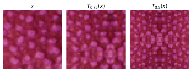
In all experiments, is implemented using the scale function from the kornia library [27], with nearest interpolation, reflection padding, aligned corners, and a different random transform-origin for each call and each element in a batch. The scale factor is uniformly sampled from . Figure 2 shows an example of transformations.
| Transform | Stop | Div2K-Train | Div2K-Val | ||
|---|---|---|---|---|---|
| PSNR | SSIM | PSNR | SSIM | ||
| Scale | ✓ | 25.9 | 0.760 | 26.3 | 0.784 |
| Shift | ✓ | 25.1 | 0.714 | 25.3 | 0.743 |
| Shift | × | 23.7 | 0.678 | 24.3 | 0.709 |
| Rotation | ✓ | 25.3 | 0.724 | 25.7 | 0.753 |
| Rotation | × | 24.2 | 0.660 | 24.7 | 0.691 |
Gradient stopping
The gradient-stopping step, which removes the dependence of on the network weights plays an important role in the self-supervised loss. Table 2 shows that gradient stopping boosts the performance of the self-supervised network in a super-resolution problem by a significant amount, i.e. 3dB. In the appendix, we demonstrate empirically that the gradient stopping technique modifies the minima of the structure compared to the standard EI technique (no stopping).
| Stop | Div2K-Train | Div2K-Val | ||
|---|---|---|---|---|
| PSNR | SSIM | PSNR | SSIM | |
| ✓ | 33.1 | 0.928 | 35.7 | 0.941 |
| × | 30.3 | 0.874 | 32.6 | 0.893 |
Comparison to self-supervision via patch recurrence
Both the proposed loss and the CSS loss in (4) leverage scale-invariance to form a self-supervised loss. The CSS method requires that is a downsampling transformation and that the noise is sufficiently small, such that for some which also belongs to the dataset. The proposed method exploits scale-invariance on the reconstructed images, thus being applicable to any operator . Thus, for the super-resolution problems with a small amount of noise, we expect to obtain a similar performance with both methods, whereas in the more challening image deblurring problem we expect to observe a different performance across methods.
5 Experiments
Dataset
Throughout the experiments, we use datasets containing pairs of ground truth images and noisy measurements. The ground truth images are obtained from Div2K [1], a dataset containing high-resolution images (around pixels) depicting natural scenes (e.g. buildings, landscapes, animals), which we resize to a resolution around pixels for image deblurring, in order to get significant degradation with reasonably small kernels. For image super-resolution, the clean measurements are computed from the ground truth images using the MATLAB function imresize, with a downsampling factor of or , bicubic interpolation and an antialiasing filter, and for image deblurring, using circular convolution with a Gaussian kernel or a box kernel. We denote the blur level by , i.e. the standard deviation for Gaussian kernels, and the radius for Box kernels. The noisy measurements are obtained by further degrading clean measurements using additive white Gaussian noise with standard deviation . Each dataset contains pairs, of which are used to train models, and which are used for validation only. Instead of training on full images, we randomly crop training patch pairs at every epoch such that input patches have size .
Network architecture
To ensure a fair comparison, all the models in the experiments are built upon the SwinIR architecture [18], which is a state-of-the-art architecture for image reconstruction. It is made of convolutional layers, but it is not fully convolutional since it also contains multi-head self-attention layers followed by a multi-layered perceptron layer. It also contains an optional upsampling layer which we use for super-resolution but not for image deblurring.
Performance metrics
We measure the reconstruction performance using the PSNR and SSIM metrics on the luminance channel (Y) in the YCbCr color space, as is often done in the image reconstruction literature [18]. We compute the reconstruction performance on training pairs, and on the validation pairs. It is important to note that computing reconstruction performance on training pairs is relevant for self-supervised methods since they do not learn from ground truth images during training.
| Div2K-Train | Div2K-Val | ||||
|---|---|---|---|---|---|
| PSNR | SSIM | PSNR | SSIM | ||
| sup | 0 | 33.3 | 0.929 | 35.9 | 0.941 |
| css | 33.2 | 0.929 | 35.9 | 0.942 | |
| proposed | 33.1 | 0.928 | 35.7 | 0.941 | |
| 30.2 | 0.883 | 32.4 | 0.900 | ||
| sup | 25/255 | 28.6 | 0.778 | 29.9 | 0.799 |
| css | 28.0 | 0.764 | 29.0 | 0.778 | |
| proposed | 28.1 | 0.786 | 29.1 | 0.802 | |
| 24.0 | 0.483 | 24.3 | 0.477 | ||
| Div2K-Train | Div2K-Val | ||||
|---|---|---|---|---|---|
| PSNR | SSIM | PSNR | SSIM | ||
| sup | 10/255 | 26.8 | 0.743 | 28.0 | 0.760 |
| css | 26.6 | 0.736 | 27.8 | 0.755 | |
| proposed | 26.5 | 0.718 | 27.6 | 0.733 | |
| 25.1 | 0.647 | 26.3 | 0.670 | ||
| sup | 25/255 | 25.3 | 0.686 | 26.3 | 0.701 |
| css | 25.2 | 0.679 | 26.1 | 0.695 | |
| proposed | 25.0 | 0.656 | 25.9 | 0.674 | |
| 22.5 | 0.449 | 23.0 | 0.459 | ||
| Div2K-Train | Div2K-Val | |||||
|---|---|---|---|---|---|---|
| PSNR | SSIM | PSNR | SSIM | |||
| sup | 1.0 | 30.8 | 0.917 | 31.0 | 0.916 | |
| proposed | 30.2 | 0.896 | 30.5 | 0.899 | ||
| css | 29.1 | 0.886 | 29.7 | 0.895 | ||
| 26.7 | 0.787 | 27.2 | 0.808 | |||
| 27.1 | 0.832 | 27.7 | 0.852 | |||
| sup | 2.0 | 26.1 | 0.773 | 26.4 | 0.795 | |
| proposed | 25.9 | 0.760 | 26.3 | 0.784 | ||
| css | 24.6 | 0.696 | 25.1 | 0.726 | ||
| 23.1 | 0.594 | 23.6 | 0.626 | |||
| 23.4 | 0.636 | 23.8 | 0.666 | |||
| sup | 3.0 | 24.1 | 0.681 | 24.3 | 0.702 | |
| proposed | 24.0 | 0.653 | 24.2 | 0.673 | ||
| css | 23.3 | 0.614 | 23.7 | 0.646 | ||
| 21.7 | 0.493 | 21.9 | 0.523 | |||
| 21.8 | 0.531 | 22.0 | 0.561 | |||
| Div2K-Train | Div2K-Val | |||||
|---|---|---|---|---|---|---|
| PSNR | SSIM | PSNR | SSIM | |||
| sup | 2 | 28.9 | 0.864 | 29.1 | 0.859 | |
| proposed | 27.8 | 0.837 | 27.9 | 0.834 | ||
| css | 26.4 | 0.796 | 26.7 | 0.806 | ||
| 23.8 | 0.620 | 24.3 | 0.661 | |||
| 24.0 | 0.661 | 24.5 | 0.701 | |||
| sup | 3 | 27.3 | 0.809 | 27.5 | 0.807 | |
| proposed | 26.0 | 0.766 | 26.3 | 0.773 | ||
| css | 24.6 | 0.703 | 25.0 | 0.726 | ||
| 22.4 | 0.529 | 22.8 | 0.565 | |||
| 22.6 | 0.568 | 22.9 | 0.603 | |||
| sup | 4 | 25.7 | 0.743 | 25.8 | 0.744 | |
| proposed | 24.8 | 0.707 | 25.1 | 0.712 | ||
| css | 23.5 | 0.627 | 23.8 | 0.657 | ||
| 21.5 | 0.469 | 21.8 | 0.501 | |||
| 21.6 | 0.506 | 21.9 | 0.538 | |||
Training details
We train models for epochs against training losses , and . We use an initial learning rate of for super-resolution, and of for deblurring. We use a multi-step scheduler that divides the learning rate by a factor of at epochs , and . We use a batch size of for super-resolution, and of for deblurring. We use the Adam optimizer [15] with and no weight decay. The experiments are performed using 4 GPUs on a SIDUS solution [23].
Super-resolution experiments
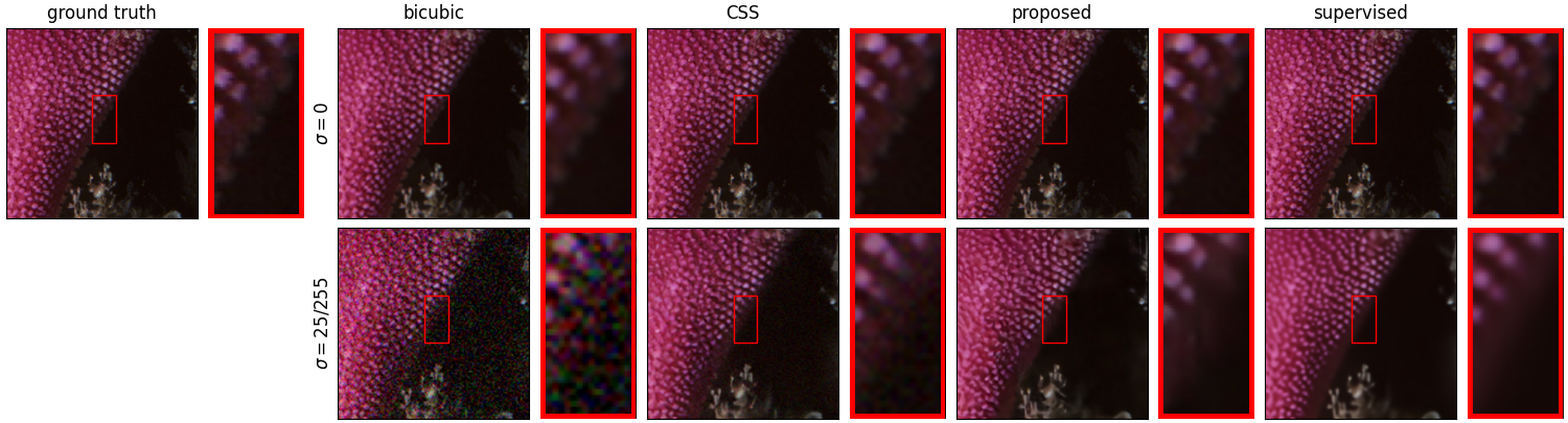
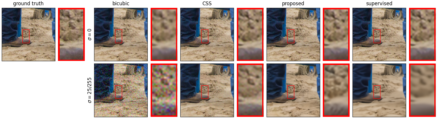
For image super-resolution, Figure 3 shows no significant visual difference between images obtained using the supervised, proposed, and CSS methods in the noiseless case. For noise level , we observe that some noise is present in the dark region on the image obtained using the CSS method, but not on those obtained using supervised and proposed methods. We also observe that the image obtained using the supervised method is slightly smoother than the ground truth image, and images obtained using the proposed and CSS methods when looking at the light pimples.
Gaussian deblurring experiments
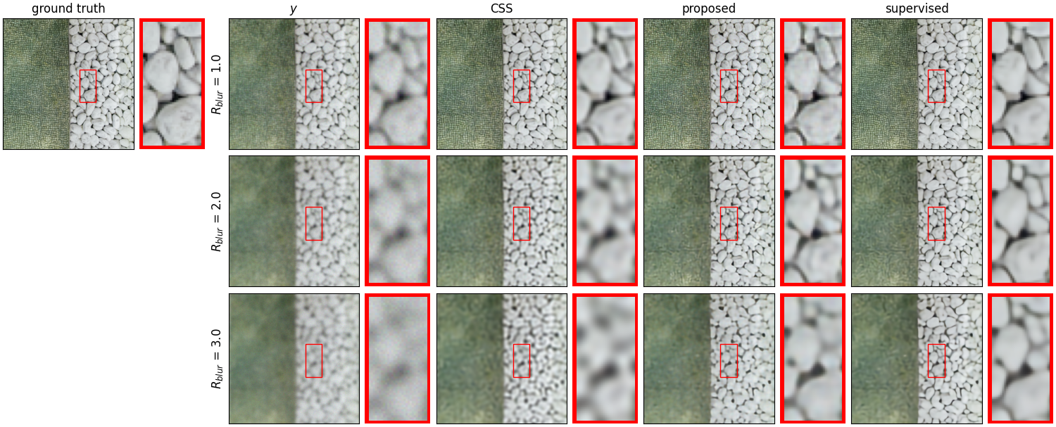
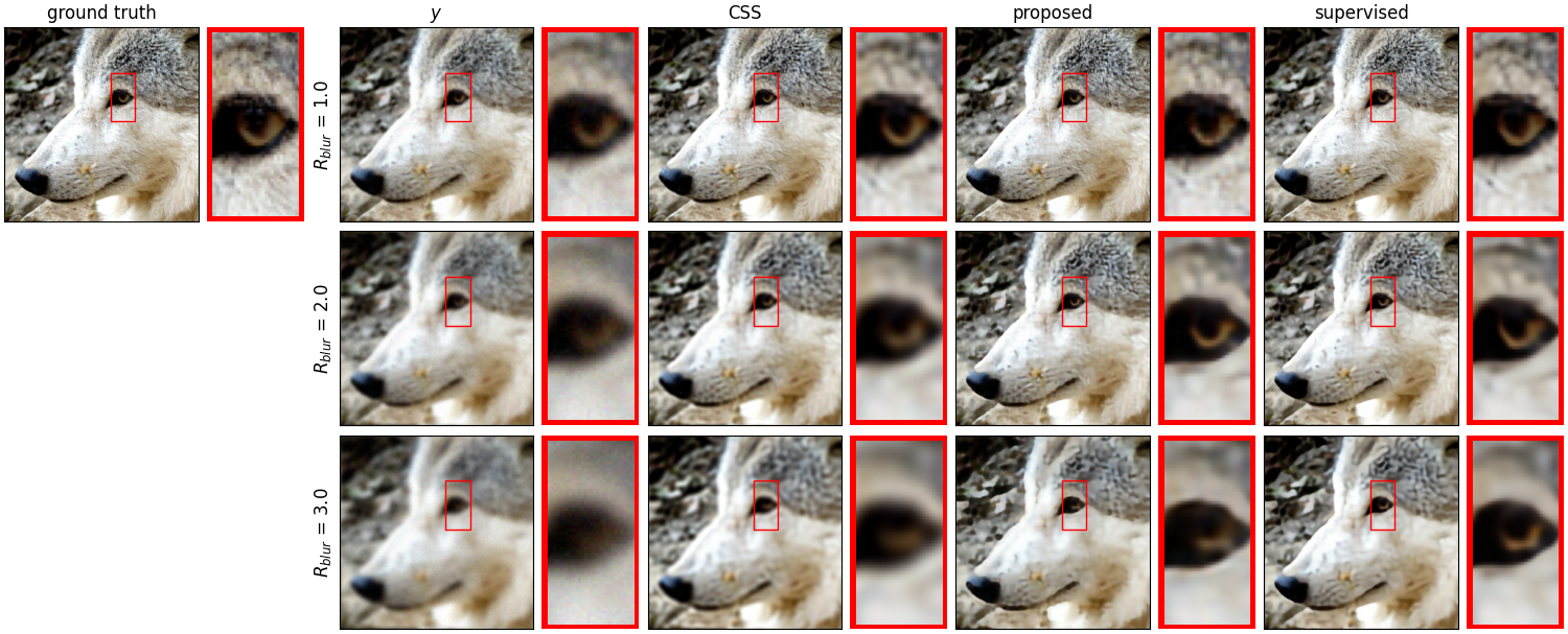
Figure 4 shows that the CSS method produces blurrier images than the supervised and proposed methods, for all three blur levels, and especially so for the two highest blur levels. For the highest blur level, we observe that the contour between two rocks on the upper right part of the zoomed-in region is visible on images obtained using the proposed and CSS methods, but is not visible on the image obtained using the supervised method.
Table 5 shows that the proposed method performs significantly better than the CSS method ( dB gain on average) and almost as good as the supervised method ( dB loss on average).
Table 1 shows that for , the proposed method (using downscaling transformations) performs better than equivariant imaging methods using shifts or rotations, even when stopping the gradient. Moreover, it shows that stopping the gradient improves the performance of the latter methods by approximately dB gain.
Box deblurring experiments
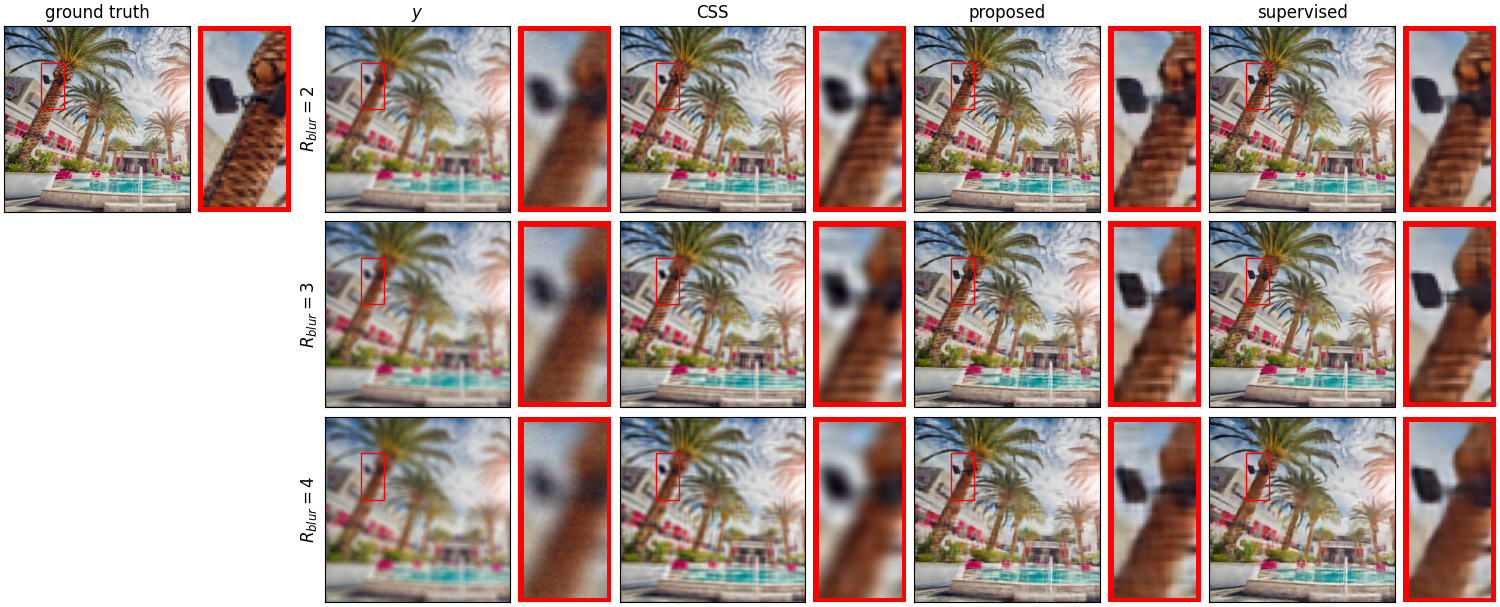
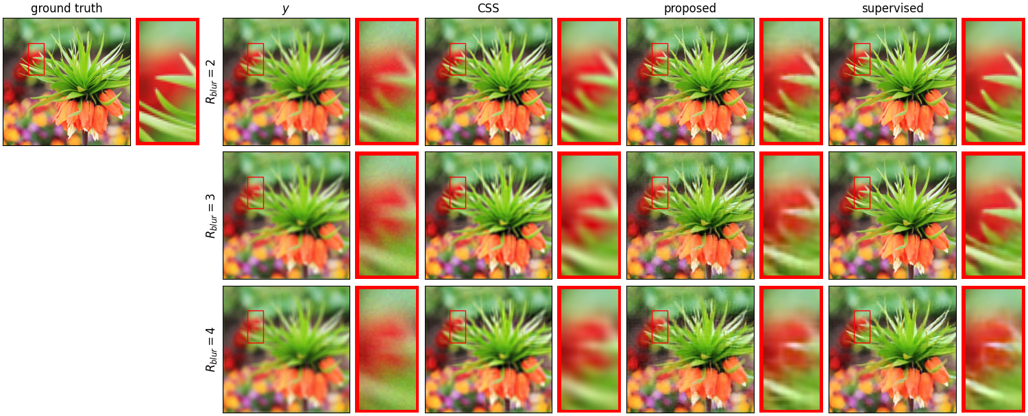
Figure 5 shows that images obtained using the CSS method are blurrier than images obtained using the supervised and proposed methods, for all three blur levels. We observe horizontal and vertical artifacts on the image obtained using the supervised method for medium blur level, on those obtained using the proposed method for medium and high levels, and on those obtained using the CSS method for all three levels, but not on other images.
Table 6 shows that the proposed method performs better than the CSS method ( dB gain on average) and dB worse than the supervised method. Overall, we observe that the proposed method performs almost as well as the supervised method, and better than the CSS method.
6 Conclusion
In this work, we propose a new self-supervised method for solving the problems of image super-resolution and image deblurring which leverages the scale-invariance of typical image distributions. The experiments show that our method can be as effective as supervised methods while outperforming other self-supervised methods.
The proposed method extends the equivariant imaging loss to problems where high-frequency information is lost, which play a fundamental role in most imaging systems. The proposed method offers significant flexibility: i) the self-supervised loss can be used to train any network architecture, ii) the loss can be applied to any inverse problem, e.g. performing super-resolution in MRI, as long as the forward process is known, and iii) only a single forward operator is required.
While a theoretical analysis of necessary and sufficient conditions for learning from measurement data alone is available for the case where the transformations are associated with a compact group, such as rotations and/or translations [30], the results do not hold for the action by scalings which form a semi-group [33] (as it does not have an inverse). The interesting question of what theoretical analysis model identification is possible in this scenario is left for future work.
References
- Agustsson and Timofte [2017] Eirikur Agustsson and Radu Timofte. NTIRE 2017 Challenge on Single Image Super-Resolution: Dataset and Study. In 2017 IEEE Conference on Computer Vision and Pattern Recognition Workshops (CVPRW), pages 1122–1131, Honolulu, HI, USA, 2017. IEEE.
- Batson and Royer [2019] Joshua Batson and Loic Royer. Noise2Self: Blind Denoising by Self-Supervision. In Proceedings of the 36th International Conference on Machine Learning, pages 524–533. PMLR, 2019. ISSN: 2640-3498.
- Belthangady and Royer [2019] Chinmay Belthangady and Loic A Royer. Applications, promises, and pitfalls of deep learning for fluorescence image reconstruction. Nature methods, 16(12):1215–1225, 2019.
- Blau and Michaeli [2018] Yochai Blau and Tomer Michaeli. The perception-distortion tradeoff. In Proceedings of the IEEE conference on computer vision and pattern recognition, pages 6228–6237, 2018.
- Bora et al. [2018] Ashish Bora, Eric Price, and Alexandros G Dimakis. Ambientgan: Generative models from lossy measurements. In International conference on learning representations, 2018.
- Chambolle and Pock [2016] Antonin Chambolle and Thomas Pock. An introduction to continuous optimization for imaging. Acta Numerica, 25:161–319, 2016.
- Chen et al. [2021] Dongdong Chen, Julian Tachella, and Mike E. Davies. Equivariant Imaging: Learning Beyond the Range Space. In 2021 IEEE/CVF International Conference on Computer Vision (ICCV), pages 4359–4368, Montreal, QC, Canada, 2021. IEEE.
- Chen et al. [2022] Dongdong Chen, Julian Tachella, and Mike E. Davies. Robust Equivariant Imaging: a fully unsupervised framework for learning to image from noisy and partial measurements. In 2022 IEEE/CVF Conference on Computer Vision and Pattern Recognition (CVPR), pages 5637–5646, New Orleans, LA, USA, 2022. IEEE.
- Dong et al. [2020] Jiangxin Dong, Stefan Roth, and Bernt Schiele. Deep Wiener Deconvolution: Wiener Meets Deep Learning for Image Deblurring. In Advances in Neural Information Processing Systems, pages 1048–1059. Curran Associates, Inc., 2020.
- Eldar [2009] Yonina C. Eldar. Generalized SURE for Exponential Families: Applications to Regularization. IEEE Transactions on Signal Processing, 57(2):471–481, 2009. Conference Name: IEEE Transactions on Signal Processing.
- Fatania et al. [2023] Ketan Fatania, Kwai Y. Chau, Carolin M. Pirkl, Marion I. Menzel, and Mohammad Golbabaee. Nonlinear Equivariant Imaging: Learning Multi-Parametric Tissue Mapping without Ground Truth for Compressive Quantitative MRI. In 2023 IEEE 20th International Symposium on Biomedical Imaging (ISBI), pages 1–4, 2023. ISSN: 1945-8452.
- Florack et al. [1992] Luc MJ Florack, Bart M ter Haar Romeny, Jan J Koenderink, and Max A Viergever. Scale and the differential structure of images. Image and vision computing, 10(6):376–388, 1992.
- Hendriksen et al. [2020] Allard A. Hendriksen, Daniel M. Pelt, and K. Joost Batenburg. Noise2Inverse: Self-supervised deep convolutional denoising for tomography. IEEE Transactions on Computational Imaging, 6:1320–1335, 2020. arXiv:2001.11801 [cs, eess, stat].
- Kamilov et al. [2023] Ulugbek S Kamilov, Charles A Bouman, Gregery T Buzzard, and Brendt Wohlberg. Plug-and-play methods for integrating physical and learned models in computational imaging: Theory, algorithms, and applications. IEEE Signal Processing Magazine, 40(1):85–97, 2023.
- Kingma and Ba [2014] Diederik P Kingma and Jimmy Ba. Adam: A method for stochastic optimization. arXiv preprint arXiv:1412.6980, 2014.
- Krull et al. [2019] Alexander Krull, Tim-Oliver Buchholz, and Florian Jug. Noise2Void - Learning Denoising From Single Noisy Images. pages 2129–2137, 2019.
- Lehtinen et al. [2018] Jaakko Lehtinen, Jacob Munkberg, Jon Hasselgren, Samuli Laine, Tero Karras, Miika Aittala, and Timo Aila. Noise2Noise: Learning Image Restoration without Clean Data. In Proceedings of the 35th International Conference on Machine Learning, pages 2965–2974. PMLR, 2018. ISSN: 2640-3498.
- Liang et al. [2021] Jingyun Liang, Jiezhang Cao, Guolei Sun, Kai Zhang, Luc Van Gool, and Radu Timofte. SwinIR: Image Restoration Using Swin Transformer. In 2021 IEEE/CVF International Conference on Computer Vision Workshops (ICCVW), pages 1833–1844, Montreal, BC, Canada, 2021. IEEE.
- Mataev et al. [2019] Gary Mataev, Peyman Milanfar, and Michael Elad. DeepRED: Deep Image Prior Powered by RED. pages 0–0, 2019.
- Metzler et al. [2020] Christopher A. Metzler, Ali Mousavi, Reinhard Heckel, and Richard G. Baraniuk. Unsupervised Learning with Stein’s Unbiased Risk Estimator, 2020. arXiv:1805.10531 [cs, stat].
- Moran et al. [2020] Nick Moran, Dan Schmidt, Yu Zhong, and Patrick Coady. Noisier2noise: Learning to denoise from unpaired noisy data. In Proceedings of the IEEE/CVF Conference on Computer Vision and Pattern Recognition, pages 12064–12072, 2020.
- Quan et al. [2022] Yuhui Quan, Zhuojie Chen, Huan Zheng, and Hui Ji. Learning Deep Non-blind Image Deconvolution Without Ground Truths. In Computer Vision – ECCV 2022, pages 642–659, Cham, 2022. Springer Nature Switzerland.
- Quemener and Corvellec [2013] Emmanuel Quemener and Marianne Corvellec. Sidus—the solution for extreme deduplication of an operating system. Linux Journal, 2013(235):3, 2013.
- Ramani et al. [2008] Sathish Ramani, Thierry Blu, and Michael Unser. Monte-carlo sure: A black-box optimization of regularization parameters for general denoising algorithms. IEEE Transactions on image processing, 17(9):1540–1554, 2008.
- Ren et al. [2020] Dongwei Ren, Kai Zhang, Qilong Wang, Qinghua Hu, and Wangmeng Zuo. Neural blind deconvolution using deep priors. In Proceedings of the IEEE/CVF Conference on Computer Vision and Pattern Recognition, pages 3341–3350, 2020.
- Ren et al. [2018] Wenqi Ren, Jiawei Zhang, Lin Ma, Jinshan Pan, Xiaochun Cao, Wangmeng Zuo, Wei Liu, and Ming-Hsuan Yang. Deep Non-Blind Deconvolution via Generalized Low-Rank Approximation. In Advances in Neural Information Processing Systems. Curran Associates, Inc., 2018.
- Riba et al. [2020] Edgar Riba, Dmytro Mishkin, Daniel Ponsa, Ethan Rublee, and Gary Bradski. Kornia: an Open Source Differentiable Computer Vision Library for PyTorch. In 2020 IEEE Winter Conference on Applications of Computer Vision (WACV), pages 3663–3672, Snowmass Village, CO, USA, 2020. IEEE.
- Shocher et al. [2018] Assaf Shocher, Nadav Cohen, and Michal Irani. Zero-Shot Super-Resolution Using Deep Internal Learning. In 2018 IEEE/CVF Conference on Computer Vision and Pattern Recognition, pages 3118–3126, Salt Lake City, UT, 2018. IEEE.
- Stein [1981] Charles M. Stein. Estimation of the Mean of a Multivariate Normal Distribution. The Annals of Statistics, 9(6):1135–1151, 1981. Publisher: Institute of Mathematical Statistics.
- Tachella and Pereyra [2023] Julian Tachella and Marcelo Pereyra. Equivariant Bootstrapping for Uncertainty Quantification in Imaging Inverse Problems, 2023. arXiv:2310.11838 [cs, eess, stat].
- Tachella et al. [2023] Julián Tachella, Dongdong Chen, and Mike Davies. Sensing Theorems for Unsupervised Learning in Linear Inverse Problems. Journal of Machine Learning Research, 24(39):1–45, 2023.
- Ulyanov et al. [2018] Dmitry Ulyanov, Andrea Vedaldi, and Victor Lempitsky. Deep Image Prior. pages 9446–9454, 2018.
- Worrall and Welling [2019] Daniel Worrall and Max Welling. Deep scale-spaces: Equivariance over scale. Advances in Neural Information Processing Systems, 32, 2019.
- Xu et al. [2014] Li Xu, Jimmy SJ Ren, Ce Liu, and Jiaya Jia. Deep Convolutional Neural Network for Image Deconvolution. In Advances in Neural Information Processing Systems. Curran Associates, Inc., 2014.
Appendix A Additional experiments
Table 7 shows that the proposed method has better performance than equivariant imaging for super-resolution with noise level .
| Transform | Stop | Div2K-Train | Div2K-Val | ||
|---|---|---|---|---|---|
| PSNR | SSIM | PSNR | SSIM | ||
| Scale | ✓ | 28.1 | 0.778 | 29.9 | 0.799 |
| Shift | ✓ | 27.7 | 0.750 | 28.6 | 0.764 |
| Shift | × | 27.6 | 0.757 | 28.8 | 0.778 |
| Rotation | ✓ | 27.9 | 0.780 | 29.0 | 0.797 |
| Rotation | × | 27.3 | 0.737 | 28.5 | 0.760 |
Appendix B Additional results
Figure 6 shows sample reconstructions for super resolution with different noise levels . Figure 7 shows sample reconstructions for Gaussian deblurring with fixed noise standard deviation and different blur levels . Figure 8 shows sample reconstructions for box deblurring with fixed noise standard deviation and different blur levels .
Appendix C Proofs of Proposition 1 and 2
In this section, we provide proofs for Proposition 1 and 2. For the sake of simplicity, we consider images with height and width equal to , although the results can be generalized for any aspect ratio. Furthermore, we write to denote the pixel in the th coordinate of , where and .
Discrete Fourier transform
We use the spectral properties of downsampling with an ideal low-pass filter, expressed in terms of the 2D discrete Fourier transform defined by
| (10) |
where .
2D circular convolutions
In order to define blur and downsampling operators, we use the 2D circular convolution of a signal by a kernel , defined by
| (11) |
where , and denotes the remainder of divided by .
Blur and downsampling operators
In this section, we consider a blur operator , defined as the 2D circular convolution by kernel ,
| (12) |
and a downsampling operator , defined by
where is the downsampling factor, , is an antialiasing kernel and . Without loss of generality, we focus on downsampling by a factor of , i.e. and , however, our results can easily be generalized for other integer factors.
Actions by shifts and rotations
The action by shifts , with horizontal and vertical displacements , is defined by
| (13) |
where , or equivalently in the Fourier basis
| (14) |
where .
The action by rotations , with angles of degrees, is defined by
| (15) |
where .
Equivariance to shifts and rotations
In this section, we prove that under mild conditions the blur operator and the downsampling operator are equivariant to actions by shifts , and by rotations . Because equivariance is a property relating an operator and a group acting on both its input and output spaces, we need to specify what group action on the output space we consider in each case. For the blur operator , input and output spaces are equal, and we consider the action on its output space to be equal to the action on its input space.
For operator and action by rotations , we consider the action on the output space to be the action by rotations , , and for the action by shifts , we consider the action on the output space to be the translation by a displacement of , defined in Fourier basis by
| (16) |
In summary, we will prove that
| (17) | |||
| (18) | |||
| (19) | |||
| (20) |
Isotropic kernels
An isotropic kernel is a kernel that is invariant to rotations, in our case it satisfies
| (21) |
Ideal anti-aliasing filter
A downsampling operator by factor with ideal anti-aliasing filter satisfies
| (22) |
where , assuming is even and is odd.
C.1 Proof of Proposition 1
We prove the proposition in two steps, first by proving that the blur operator is equivariant to shifts, then that it is equivariant to rotations as long as the kernel is isotropic.
Let and . Using (12) and Lemma 1, we compute
| (23) | ||||
| (24) | ||||
| (25) |
Thus the blur operator is equivariant to shifts.
Now, we assume that is an isotropic kernel, and let . Using (12) and Lemma 2 we compute
| (26) | ||||
| (27) |
where . Then using (21) and (12) we compute
| (28) | ||||
| (29) |
Thus the blur operator is equivariant to shifts.
Lemma 1.
For , and
| (30) |
Proof.
Let ,
| (31) | ||||
| (32) | ||||
| (33) | ||||
| (34) |
∎
Lemma 2.
For , and ,
| (35) |
where .
C.2 Proof of Proposition 2
We start by proving that the downsampling operator with anti-aliasing filter is equivariant to shifts, then we prove it is equivariant to rotations.
| (43) | |||
| (44) | |||
| (45) | |||
| (46) |
Thus, the operator is equivariant to shifts.
| (47) | ||||
| (48) | ||||
| (49) | ||||
| (50) | ||||
| (51) |
Thus, the operator is equivariant to rotations.
Lemma 3.
For
| (52) |
where .
Proof.
If , then and (52) is satisfied. If , let , and . We compute
| (53) | ||||
| (54) | ||||
| (55) | ||||
| (56) | ||||
| (57) | ||||
| (58) |
thus . If or , we prove similarly as in the case. ∎
Lemma 4.
For , , and ,
| (59) |
Appendix D Proof of Theorem 1
In this section, we prove that blurring and downsampling with an ideal anti-aliasing filter is not equivariant to downscaling. Since an ideal anti-aliasing filter is a special case of blurring operator, it suffices to prove that blurring is not equivariant to downscaling, i.e. that for a signal , and a scaling factor ,
| (63) |
Without loss of generality, we prove the theorem for 1D signals. Extending the results to 2D signals is straightforward. We also assume that is odd.
Blur transfer function
The Fourier transform of a blur filter is typically nonzero around the zero-frequency, and in particular as long as the number of samples is large enough,
| (64) |
Moreover, if the blur operator is not invertible, its Fourier transform vanishes for some frequency ,
| (65) |
Symmetry of real filters
Throughout the proof, we use the symmetry property of real filters (note that we work with real forward operators ), which satisfy
| (66) |
where denote the complex conjugate of .
Action by downscalings
Downscaling in space consists of upscaling in frequency, in particular, a downscaling by a factor satisfies that
| (67) |
where , and is a Dirac vector positioned at , i.e. if , and otherwise.