Dirichlet-based Uncertainty Quantification
for Personalized Federated Learning
with Improved Posterior Networks

Abstract

In modern federated learning, one of the main challenges is to account for inherent heterogeneity and the diverse nature of data distributions for different clients. This problem is often addressed by introducing personalization of the models towards the data distribution of the particular client. However, a personalized model might be unreliable when applied to the data that is not typical for this client. Eventually, it may perform worse for these data than the non-personalized global model trained in a federated way on the data from all the clients. This paper presents a new approach to federated learning that allows selecting a model from global and personalized ones that would perform better for a particular input point. It is achieved through a careful modeling of predictive uncertainties that helps to detect local and global in- and out-of-distribution data and use this information to select the model that is confident in a prediction. The comprehensive experimental evaluation on the popular real-world image datasets shows the superior performance of the model in the presence of out-of-distribution data while performing on par with state-of-the-art personalized federated learning algorithms in the standard scenarios.

1 Introduction

The widespread adoption of deep neural networks in various applications requires reliable predictions, which can be achieved through rigorous uncertainty quantification. Although uncertainty quantification has been extensively studied in different domains under centralized settings (Lee et al., 2018; Lakshminarayanan et al., 2017; Gal & Ghahramani, 2016), only a few works have considered this area within the context of federated learning (Linsner et al., 2022; Kotelevskii et al., 2022). Typically, in federated learning papers, algorithms result in using either a personalized local model or a global model. However, both these models could be useful in different cases by providing the tradeoff between personalization of a local model and higher reliability of the global one (Hanzely & Richtárik, 2020; Liang et al., 2019).
In this paper, we introduce a new framework to choose whether to predict with a local or global model at a given point based on uncertainty quantification. The core idea is to apply the global model only if the local one has high epistemic (model) uncertainty (Hüllermeier & Waegeman, 2021) about the prediction at a given point, i.e., the local model doesn’t have enough information about the particular input point. In case the local model is confident (either in predicting a particular class or in the fact that it is observing an ambiguous object with high aleatoric (data) uncertainty (Hüllermeier & Waegeman, 2021)), it should make the decision itself without involving the global one.
As a specific instance of our framework, we propose an approach inspired by Posterior Networks (PostNet; Charpentier et al. (2020)) and its modification, Natural Posterior Networks (NatPN; Charpentier et al. (2022)). This type of model is particularly useful for our purposes, as it enables the estimation of aleatoric and epistemic uncertainties without incurring additional inference costs. Thus, we are able to fully implement the switching between local and global models in an efficient way.
Related work. The literature presents various approaches to uncertainty quantification in federated learning settings. In (Linsner et al., 2022), the authors suggest that training an ensemble of $K$ global models is the most effective for federated uncertainty quantification. Despite its effectiveness, this approach is $K$ times more expensive compared to the classic FedAvg method. Another proposal comes from (Kotelevskii et al., 2022), where the authors recommend using Markov Chain Monte Carlo (MCMC) to obtain samples from the posterior distribution. However, this method is practically almost infeasible due to its significant computational complexity.
Other works, such as (Chen & Chao, 2021; Kim & Hospedales, 2023), also present methods that could potentially estimate uncertainty in federated learning. However, these papers do not expressly address the opportunities and challenges of uncertainty quantification in their discussion. It’s important to note that there are existing approaches of deferring classification to other models or experts in case of abstention, for example (Keswani et al., 2021). Despite this, none of these approaches have been explored in a federated context, nor have they considered the corresponding constraints.
The central idea of PostNet and NatPN involves using a Dirichlet prior and posterior distributions over the categorical predictive distributions (Malinin & Gales, 2018; 2019; Charpentier et al., 2020; 2022; Sensoy et al., 2018). To parameterize the parameters of these Dirichlet distributions, the authors suggest introducing a density model over the deep representations of input objects. In NatPN, a Normalizing Flow (Papamakarios et al., 2021; Kobyzev et al., 2020) is employed to estimate the density of embeddings extracted by a trained feature extractor. This density is then used to calculate updates to the Dirichlet distribution.
Despite the success of the NatPN model (Charpentier et al., 2022), we identified certain issues with the loss function employed in NatPN, which become particularly critical when dealing with high aleatoric uncertainty regions. Intriguingly, the issue was not discovered in the authors’ recent work (Charpentier et al., 2023), which investigated potential issues in the training procedure. Recent works (Bengs et al., 2022; 2023) have unveiled other potential issues related to the training of Dirichlet models in general but have not offered solutions to address these challenges.
Contributions. Our paper stands out as one of the few studies that specifically addresses the problem of uncertainty quantification in federated learning. We aim to provide a comprehensive analysis of this important topic, considering both theoretical and practical aspects, and presenting solutions that overcome the limitations of existing approaches in the literature. The contributions of this paper are as follows:

1. We present a new federated learning framework that is based on uncertainty quantification, which allows switching between using a personalized local or global model. To achieve that, we consider several types of uncertainties for local and global models and propose a procedure that ensures that the model is confident in its prediction if the prediction is made. Otherwise, our framework rejects the prediction if we are confident that there is a high uncertainty in the predicted class.

2. We introduce a specific realization of our framework FedPN, using Dirichlet-based NatPN model. For this particular model, we identify an issue in the loss function of NatPN (not known in literature before) that complicates disentanglement of aleatoric and epistemic uncertainties, and propose a solution to rectify it.

3. We conduct an extensive set of experiments that demonstrate the benefits of our approach for different input data scenarios. In particular, we show that the proposed model outperforms state-of-the-art personalized federated learning algorithms in the presence of out-of-distribution date, while being on par with them in standard scenarios.

2 General framework of switching between global and personal models

In this section, we introduce our framework, discussing the general idea and potential nuances. In the subsequent section, we will delve into a specific implementation.

2.1 Concept overview

We are going to consider a federated learning setting with multiple clients, each having its own personalized local model. However, we additionally assume that the global model is available. The global model is typically expected to perform reasonably well on each client’s data. Assuming that we already have trained global and local models, we consider a situation where clients have the option to use either the global model or their local models to make predictions for a new incoming object $x$.
The choice between local and global models for prediction depends on the multiple factors that contribute to their prediction quality. First of all, shift in the distribution between the local data of a particular client and the global population may have significant effect on the models’ performance. Possible shifts include covariate shift, label shift or different types of label noise. If the shift is significant, the global model might be very biased with respect to the prediction for the particular client, while normally the local model is unbiased.

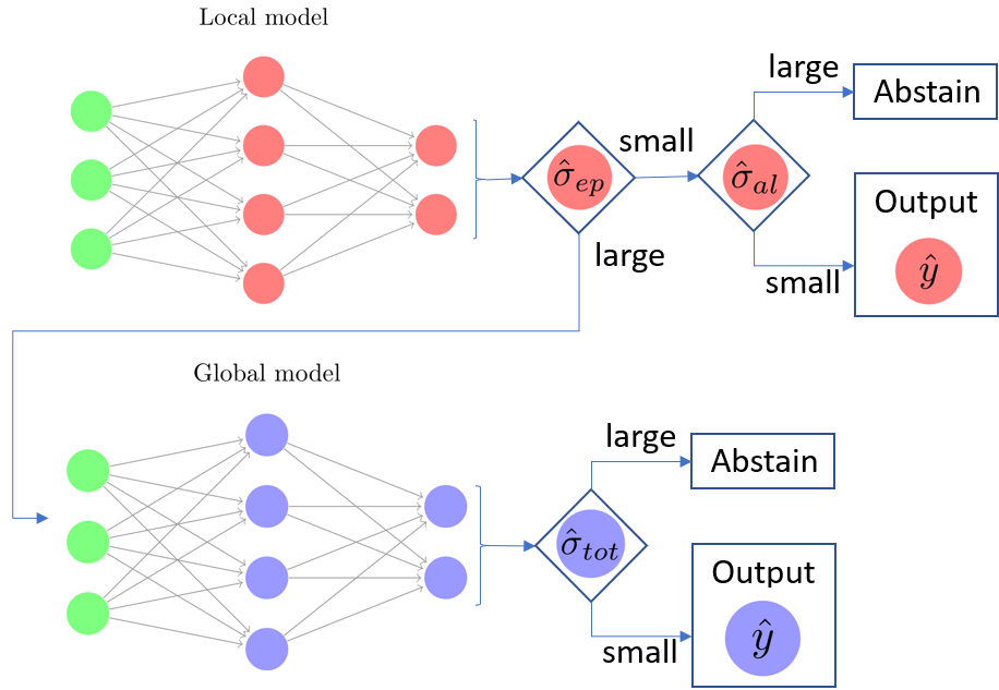
Figure 1: The general scheme of the proposed approach. Each input is first processed by personalized local model. In case of high epistemic uncertainty, the decision is delegated to the global model. Otherwise, if epistemic uncertainty is low, local model proceeds with the decision. Both models consider also aleatoric uncertainty and may abstain from prediction.

The second part of the picture is the size of the available data. Generally, the global model has more data and potentially, if no data shift is present, should outperform the local one. However, the global model is usually trained with no direct access to the data stored at clients, which might degrade its performance. Eventually, the best performing model will be the one which achieves better bias variance trade-off.
In this work, we propose a framework to choose between the pointwise usage of a local or global model for prediction. This decision is based on the uncertainty scores provided by the model. This approach aims to mitigate issues that arise when there is a distribution shift between a client’s distribution and the global distribution, which can often hinder model performance. By using uncertainty to guide the model selection, we can enhance the model’s ability to perform well even in the presence of such distribution shifts.
Both the local and global models can provide uncertainty estimates. These estimates include not only the total predictive uncertainty but also separately aleatoric and epistemic uncertainties. This feature allows for a more refined decision-making process, ensuring the most suitable model is used for prediction or choosing to abstain from making a prediction altogether in the face of high uncertainty. The resulting workflow is summarized in Figure 1.

2.2 Optimal choice of model

We start from the important fact that the local model is not exposed to the data shift between the general population and the particular client. Thus, if this model is sufficiently confident in the prediction, there is no need to involve the global model at all. However, it is important to distinguish between different types of uncertainty here. Usually, the total uncertainty of the model predicting at a particular data point can be split into two parts: aleatoric uncertainty and epistemic uncertainty (Hüllermeier & Waegeman, 2021). Aleatoric uncertainty is the one that reflects the inherent randomness in the data labels. The epistemic uncertainty is the one that reflects the lack of knowledge due to the fact that the model was trained on a data set of a limited size, or model misspecification. In what follows we will refer to epistemic as to “lack of knowledge” uncertainty, as the models we are using, neural networks, are known to be very flexible.
For our problem, it is extremely important to distinguish between aleatoric and epistemic uncertainties. Suppose the local model has low epistemic and high aleatoric uncertainty at some point. In that case, the model is confident that the predicted label is ambiguous, and the model should abstain from prediction. However, if the epistemic uncertainty is high, it means that the model doesn’t have enough knowledge to make the prediction (not enough data), and the global model should make the decision. The global model, in its turn, may either proceed with the prediction if it is confident or abstain from prediction if there is high uncertainty associated with the prediction. Thus, in this context, for a fixed client and an unseen input, there are four interesting outcomes, see Table 1. Note, that when local epistemic uncertainty is low, there is no need to refer to the global model. The inherent assumption here is that the local model is better than the global one if it knows the input point well. Thus we consider only two options for the local model: low epistemic with low aleatoric and low epistemic with high aleatoric regardless of the confidence of the global model. When the local epistemic uncertainty is high, it means that the client barely knows the input point, and thus we refer to the global model. For the global model, we look at the total uncertainty as we only care about the error of prediction which is determined by total uncertainty.

Known knowns	Known unknowns
Local Confident. This represents local in-distribution data for which the local model is confident in prediction.	Local Ambiguous. This is local in-distribution data with high aleatoric uncertainty (class ambiguity).
Unknown knowns	Unknown unknowns
Local OOD. This refers to data that is locally unknown (high epistemic uncertainty) but known to other clients. In this case, it makes sense to use the global model for predictions.	Global Uncertain. These input data is out-of-distribution for the local model while the global model is uncertain in prediction (high total uncertainty). The best course of action is to abstain from making a prediction.

Table 1: Possible scenarios for the input data point in the introduced setup. A particular input falls in one of the categories depending on the confidence in its prediction by local and global models. The disentanglement between aleatoric and epistemic uncertainties is crucial to make the decision in an optimal way.

The particular implementation of the approach described above would depend on the choice of the machine learning model and the way to compute uncertainty estimates. The key feature required is the ability of the method to compute both aleatoric and epistemic uncertainties. In the next section, we propose the implementation of the method based on the posterior networks framework (Charpentier et al., 2020).

3 Dirichlet-based deep learning models

We have chosen to showcase Dirichlet-based models (Malinin & Gales, 2018; Charpentier et al., 2020; 2022) as a specific instance of our general framework. The intuition behind this decision lies in the fact that these models allow the distinction between various types of uncertainty and facilitate the computation of corresponding uncertainty estimates with minimal additional computational overhead. Furthermore, unlike ensemble methods (Beluch et al., 2018), there is no need to train multiple models. In comparison to approximate Bayesian techniques, such as MC Dropout (Gal & Ghahramani, 2016), Variational Inference (Graves, 2011) or MCMC (Izmailov et al., 2021), almost all expectations of interest can be derived in closed form and almost without computational overhead. This makes Dirichlet-based models an attractive and efficient option for implementing our proposed framework.

3.1 Basics of Dirichlet-based models

In this section, we introduce the basics of Dirichlet-based models for classification tasks. To ease the introduction, let us start by considering a training dataset $D=\{x_{i},y_{i}\}_{i=1}^{N}$, where $N$ denotes the total number of data points in the dataset. We assume that labels $y_{i}$ belong to one of the $K$ classes.
Typically, the Dirichlet-based approaches assume that the model consists of two hierarchical random variables, $\bm{\mu}$ and $\theta$. The posterior predictive distribution for a given unseen object $x$ can be computed as follows:

$$p(y\mid x,D)={\int}p(y\mid\bm{\mu})\left[{\int}p(\bm{\mu}\mid x,\theta)~{}p(\theta\mid D)d\theta\right]d\bm{\mu},$$

where $p(y\mid\bm{\mu})$ is the distribution over class labels, given some probability vector (e.g., Categorical), $p(\bm{\mu}\mid x,\theta)$ is the distribution over a simplex (e.g., Dirichlet), and $p(\theta\mid D)$ is the posterior distribution over parameters of the model.
However, for practical neural networks, the posterior distribution $p(\theta\mid D)$ does not have an analytical form and is computationally intractable. Following (Malinin & Gales, 2018), we suggest considering “semi-Bayesian” scenario by looking on a point estimate of this distribution: $p(\theta\mid D)=\delta(\theta-\hat{\theta})$, where $\hat{\theta}$ is some estimate of the parameters (e.g., MAP estimate). Then the integral inside the brackets simplifies:

$${\int}p(\bm{\mu}\mid x,\theta)~{}p(\theta\mid D)d\theta={\int}p(\bm{\mu}\mid x,\theta)~{}\delta(\theta-\hat{\theta})d\theta=p(\bm{\mu}\mid x,\hat{\theta}).$$

In the series of works (Malinin & Gales, 2018; 2019; Charpentier et al., 2020; 2022) the posterior distribution $p(\bm{\mu}\mid x,\hat{\theta})$ is chosen to be the Dirichlet distribution $\textit{Dir}\bigl{(}\bm{\mu}\mid\bm{\alpha}^{\text{post}}(x)\bigr{)}$ with the parameter vector $\bm{\alpha}^{\text{post}}(x)=\bm{\alpha}^{\text{post}}(x\mid\hat{\theta})$ that depends on the input point $x$. In these models, the prior over probability vectors $\bm{\mu}$ takes the form of a Dirichlet distribution, representing the distribution over our beliefs about the probability of each class label. In other words, it is a distribution over distributions of class labels. This prior is parameterized by a parameter vector $\bm{\alpha}^{\text{prior}}$, where each component $\alpha^{\text{prior}}_{c}$ corresponds to our belief in a specific class. PostNet (Charpentier et al., 2020) and NatPN (Charpentier et al., 2022) propose the idea that the posterior parameters $\bm{\alpha}^{\text{post}}(x)$ can be computed in the form of pseudo-counts that are computed by a function:

$$\bm{\alpha}^{\text{post}}(x)=\bm{\alpha}^{\text{prior}}+\bm{\alpha}(x),$$ (1)

where $\bm{\alpha}(x)=\bm{\alpha}(x\mid\hat{\theta})$ is a function of input object $x$ that maps it to positive values.
Parameterization of $\bm{\alpha}(x)$. In NatPN it is proposed to use the following parameterization:

$$\bm{\alpha}(x)=p\bigl{(}g(x)\bigr{)}\bm{f}\bigl{(}g(x)\bigr{)}.$$ (2)

In this parameterization, $g(x)$ represents a feature extraction function that maps the input object $x$ (usually high-dimensional) to a lower-dimensional embedding. Subsequently, $p(\cdot)$ is a “density” function (parameterized by normalizing flow in the case of (Charpentier et al., 2022; 2020)), and $\bm{f}(\cdot)$ is a function mapping the extracted features to a vector of class probabilities.
This parameterization offers several advantages. Firstly, since $p(\cdot)$ is expected to represent the density of training examples, it should be high for in-distribution data. Secondly, as the density is properly normalized, embeddings that lie far from the training ones will result in lower values of $p\bigl{(}g(x)\bigr{)}$, thus leading to lower $\bm{\alpha}(x)$. This means that for such input $x$, we will not add any evidence, and consequently, $\bm{\alpha}^{\text{post}}(x)$ will be close to $\bm{\alpha}^{\text{prior}}$.

3.2 Uncertainty measures for Dirichlet-based models

One of the advantages of using Dirichlet-based models is their ability to easily disentangle and quantitatively estimate aleatoric and epistemic uncertainties.
Epistemic uncertainty. We begin by discussing epistemic uncertainty, which can be estimated in multiple different ways (Malinin & Gales, 2021). In this work, following the ideas from (Malinin & Gales, 2018), we quantify the epistemic uncertainty as the entropy of a posterior Dirichlet distribution, which can be analytically computed as follows

$$\mathcal{H}[\textit{Dir}\bigl{(}\bm{\mu}\mid\bm{\alpha}^{\text{post}}(x)\bigr{)}]=\ln\tfrac{\prod_{i=1}^{K}\Gamma\bigl{(}\alpha^{\text{post}}_{i}(x)\bigr{)}}{\Gamma\bigl{(}\alpha^{\text{post}}_{0}(x)\bigr{)}}-\textstyle{\sum}_{i=1}^{K}(\alpha^{\text{post}}_{i}(x)-1)(\tilde{\psi}\bigl{(}\alpha^{\text{post}}_{i}(x)\bigr{)}-\tilde{\psi}\bigl{(}\alpha^{\text{post}}_{0}(x)\bigr{)}),$$ (3)

where $\bm{\alpha}^{\text{post}}(x)=\bigl{[}\alpha^{\text{post}}_{1}(x),\dots,\alpha^{\text{post}}_{K}(x)\bigr{]}$, $\tilde{\psi}$ is a digamma function and $\alpha^{\text{post}}_{0}(x)=\sum_{i=1}^{K}\alpha^{\text{post}}_{i}(x)$.
Aleatoric uncertainty. Aleatoric uncertainty can be measured using the average entropy (Kendall & Gal, 2017), which can be computed as follows:

$$\mathbb{E}_{\bm{\mu}\sim\textit{Dir}\bigl{(}\bm{\mu}\mid\bm{\alpha}^{\text{post}}(x)\bigr{)}}\mathcal{H}[p(y\mid\bm{\mu})]=-\textstyle{\sum}_{i=1}^{K}\tfrac{\alpha^{\text{post}}_{i}(x)}{\alpha^{\text{post}}_{0}(x)}[\tilde{\psi}\bigl{(}\alpha^{\text{post}}_{i}(x)+1\bigr{)}-\tilde{\psi}\bigl{(}\alpha^{\text{post}}_{0}(x)+1\bigr{)}].$$ (4)

This metric captures the inherent noise present in the data, thus providing an estimate of the aleatoric uncertainty.

3.3 Loss functions for Dirichlet-based models

The loss function used in (Charpentier et al., 2022; 2020) is the expected cross-entropy, also known as Uncertain Cross Entropy (UCE) (Biloš et al., 2019). Note, that this loss function is a strictly proper scoring rule, which implies that a learner is incentivized to learn the true conditional $p(y\mid x)$. For a given input $x$, the loss can be written as:

$$L(y,\bm{\alpha}^{\text{post}}(x))=\mathbb{E}_{\bm{\mu}\sim\textit{Dir}\bigl{(}\bm{\mu}\mid\bm{\alpha}^{\text{post}}(x)\bigr{)}}\textstyle{\sum}_{i=1}^{K}-\mathds{1}[y=i]\log\mu_{i}=\\ \mathbb{E}_{\bm{\mu}\sim\textit{Dir}\bigl{(}\bm{\mu}\mid\bm{\alpha}^{\text{post}}(x)\bigr{)}}\text{CE}(\bm{\mu},y)=\tilde{\psi}\bigl{(}\alpha^{\text{post}}_{0}(x)\bigr{)}-\tilde{\psi}\bigl{(}\alpha^{\text{post}}_{y}(x)\bigr{)},$$ (5)

where $\alpha^{\text{post}}_{0}(x)=\sum_{i=1}^{K}\alpha^{\text{post}}_{i}(x)$. Additionally, authors suggest to penalize too concentrated predictions, by adding the regularization term with some hyperparameter $\lambda$. The overall loss function looks as follows:

$$L(y,\bm{\alpha}^{\text{post}}(x))-\lambda\mathcal{H}[\textit{Dir}\bigl{(}\bm{\mu}\mid\bm{\alpha}^{\text{post}}(x)\bigr{)}],$$ (6)

where $\mathcal{H}$ denotes the entropy of a distribution. This overall loss function referred by authors as Bayesian loss (Charpentier et al., 2022; 2020).
Issue with the loss function. Let us explore an asymptotic form of (5). For all $x>0$, the following inequality holds:

$$\log x-\tfrac{1}{x}\leq\tilde{\psi}(x)\leq\log x-\tfrac{1}{2x}.$$

Recalling the update rule (1) and using the specific parameterization of $\alpha^{\text{prior}}_{c}=1$ for all $c$, we conclude that all $\alpha^{\text{post}}_{c}(x)>1$. Hence, we can approximate $\tilde{\psi}\bigl{(}\alpha^{\text{post}}_{c}(x)\bigr{)}\approx\log\alpha^{\text{post}}_{c}(x)$.
To simplify the notation, we will use $z=g(x)$ and denote by $f_{y}(z)$ predicted probability for the $y$-th (correct) class:

$$L(y,\bm{\alpha}^{\text{post}}(x))\approx\log(\alpha^{\text{post}}_{0}(x))-\log(\alpha^{\text{post}}_{y}(x))=\log K+\log\big{[}1+\tfrac{p(z)(\tfrac{1}{K}-f_{y}(z))}{\alpha^{\text{prior}}_{y}+p(z)f_{y}(z)}\big{]},$$ (7)

see the full derivation in Supplementary Material (SM), Section A.2.
We observe from (7) that for an in-distribution case with high aleatoric uncertainty (when all classes are confused and equally probable), the last term is canceled. Note, that the presence of entropy term (that is used in (Charpentier et al., 2022; 2020) resulting to the final loss of equation (6)), which incentivizes learner to produce smooth prediction will only amplify the effect. This implies that no gradients concerning the parameters of the density model will be propagated. As a result, $p(\cdot)$, which is the density in the embedding space, may disregard regions in the embedding space that correspond to areas with a high concentration of ambiguous training examples. This violates the intuition of $p(\cdot)$ as a data density. Thus, uncertainty estimates based on $p(\cdot)$ cannot be used to measure epistemic uncertainty, as it ignores the regions with high aleatoric uncertainty.

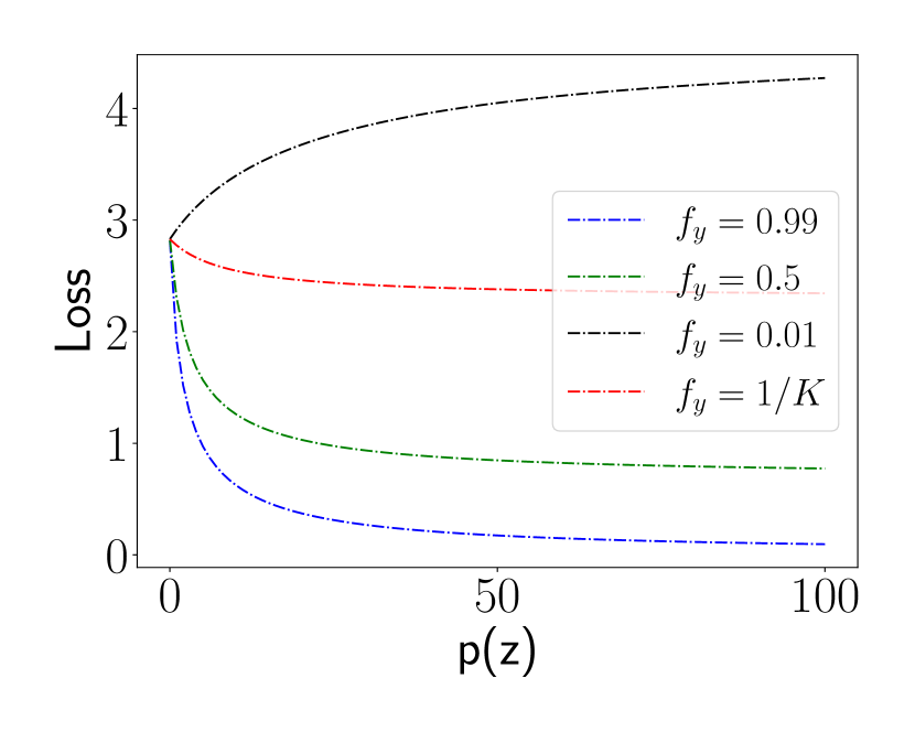
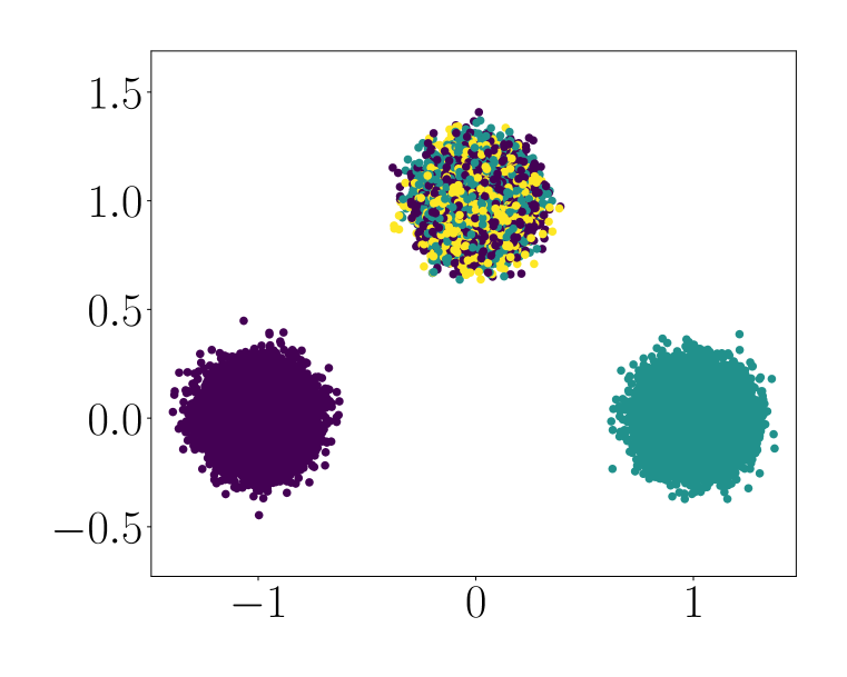
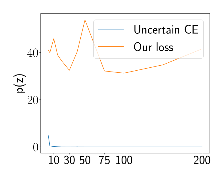
Figure 2: Left: Image depicts the landscape of the loss function with $K=10$ classes. The red line (representing high aleatoric regions) appears relatively flat. Even at this level, the density in corresponding points tends to be underestimated. As the number of classes increases, this effect is amplified. Center: This image depicts the training data, where the leftmost and rightmost Gaussians consist of only one class each. In contrast, the middle Gaussian contains all $K$ labels, randomly permuted. Each Gaussian has an equal number of data points, implying that, if $p(z)$ follows the intuition of density, all peaks should have the same height. Right: By altering the number of classes $K$, we change the aleatoric uncertainty. We train the model using the vanilla approach of NatPN and measure $p(z)$ at the central peak. As the number of classes increases, the density for UCE decreases, violating the intuition that $p(z)$ is the density of training data. While for our proposed trick it behaves as expected.

In addition to the problem of confusing high-aleatoric and high-epistemic regions, we discovered that the proposed loss function defy intuition when confronted with “outliers.” We define an “outlier” as an object with a predicted probability of the correct class is less than $\frac{1}{K}$. From (7), we observe that the last term changes its sign precisely at the point where $f_{y}(z)=\frac{1}{K}$. This implies that to minimize the loss function, we must decrease $p(z)$ at these points, which seems counterintuitive since these $z$ values correspond to objects from our training data.
Although the issue concerning equation (5) arises primarily in the asymptotic context, we can readily illustrate it through the loss function profiles (see Figure 2-left) for a range of fixed correct class prediction probabilities.
To further emphasize the problem, we examine the loss function landscape and provide a demonstrative example. Consider three two-dimensional Gaussian distributions, each with a standard deviation of $0.1$ and centers at $(-1,0),(1,0)$, and $0,1)$ (see Figure 2-center). Left and right clusters are set to include objects of only one class, while the middle distribution contains uniformly distributed labels, representing a high aleatoric region. Each Gaussian contains an equal amount of data. We train the NatPN model using a centralized approach, employing both the loss function from equation (5) and the loss function with out fix; see equation (8). Subsequently, we evaluate the quality of the learned model by plotting the density in the center of middle Gaussian. Ideally, we would expect the density to be equal for different number of classes $K$. However, we observe the different picture with “density” estimate at the central cluster decreasing when one increases the number of clusters, see Figure 2-right. In this Figure, we plot the median of the estimated density for different loss functions. We see, that our simple fix rectifies the behaviour of the loss function. We refer reader to additional toy example on image data in Appendix, Section B.5.
It is essential to emphasize that addressing these issues is critical for our framework, as we need to accurately differentiate between aleatoric and epistemic uncertainties in order to select the appropriate model for a given situation. Consequently, in the following section, we propose a simple but efficient technique to rectify the aforementioned problem with the loss function, ensuring that our framework effectively distinguishes between the different types of uncertainties and makes informed model choices.
Proposed solution. We propose to still use parametric model to estimate density, but now our goal is to ensure that $p(\cdot)$ accurately represents the density of our training embeddings. To achieve this, we propose maximizing the likelihood of the embeddings explicitly by incorporating a corresponding term into the loss function. Simultaneously, we aim to prevent any potential impact of the Bayesian loss on the density estimation parameters, maintaining their independence.

Thus, we suggest the following loss function:

$$L\bigl{(}y,\text{StopGrad}_{p(g(x))}\bm{\alpha}^{\text{post}}(x)\bigr{)}-\lambda\mathcal{H}\bigl{[}\textit{Dir}\bigl{(}\bm{\mu}\mid\bm{\alpha}^{\text{post}}(x)\bigr{)}\bigr{]}-\gamma\log p\bigl{(}g(x)\bigr{)},$$ (8)

where $\lambda,\gamma>0$ are hyperparameters, and $\text{StopGrad}_{p(g(x))}$ means that the gradient will be not propagated to the parameters of a density model, which parameterizes $p\bigl{(}g(x)\bigr{)}$.

We should note that while the corrected loss function is indeed somewhat ad hoc, it is computationally simple and very straightforward to implement, which is very important for modern deep learning. Compared to the original loss function, our rectified loss does not introduce any additional computational overhead – in both cases (for the old loss and the new one) the gradient will be computed only once with respect to each of the parameters.

4 FedPN: Specific instance of the framework

4.1 Federated setup

In this section we show, how one can adapt NatPN for federated learning.

Suppose we are given an array of datasets $D_{i}$ for $1\leq i\leq b$, where $b$ represents the number of clients. Each $D_{i}=\{x^{i}_{j}\in\mathbb{R}^{d},y^{i}_{j}\}_{j=1}^{|D_{i}|}$ consists of object-label pairs. We construct our federated framework in such a way that all clients share the feature extractor $g$ parameters $\phi$ and maintain personalized heads $f^{i}$ parameterized by $\theta_{i}$. Furthermore, we retain a “global” head-model $f$, which is trained using the FedAvg (McMahan et al., 2017) method and which ultimately has parameters $\theta$.
Following the NatPN approach, we employ normalizing flows to estimate the embedding density. As it is for head models, here we also learn two types of models – a local density models $p^{i}$ (using local data) parameterized by $\psi_{i}$ and global density model $p$ (using data from other clients in a federated fashion) parameterized by $\psi$. It is important to note that both types of models are trained on the same domain since the feature extractor model is fixed for local and global models. We refer readers to Appendix, Section B.2 for the discussion of computational overhead.

4.2 Threshold selection

Before discussing the results, it is essential to understand how we determine whether to make predictions using a local model or a global one.
This decision, resulting in a “switching” model, depends on a particular uncertainty score. This score can either be the logarithm of the density of embeddings, obtained using the density model (normalizing flows), or the entropy of predictive Dirichlet distribution (3). We found that both measures provide comparable behaviour, and in the experiments for the Table 2 we use density of embeddings.
To apply this approach, we must establish a rule for how a client decides whether to use its local model for predictions on a previously unseen input object $x$ or to delegate the prediction to the global model. One approach is to select some uncertainty values’ threshold. This threshold can be chosen based on an additional calibration dataset. In our experiments, we split each client’s validation dataset in a 40/60 ratio, using the smaller part for calibration. Note that the calibration dataset only includes those classes used during the training procedure.
The choice of the threshold is arguably the most subjective part of the approach. Ideally, we would desire to have access to explicit out-of-distribution data (either from other client “local OOD” or completely unrelated data “global OOD”). With this data, we could explicitly compute uncertainty scores for both types of data (in-distribution and out-of-distribution) and select the threshold that maximizes accuracy. However, we believe it is unfair to assume that we have this data in the problem statement. Therefore, we suggest a procedure for choosing the threshold based solely on available local data.
To choose the threshold, we assume that for all clients, there might be a chance that some $p\%$ (typically 10%) of objects considered as outliers. We further compute the estimates of epistemic uncertainty (with either entropy or the logarithms of density of embeddings) and select an appropriate threshold based on this assumption for each of the clients. For the high epistemic uncertainty points of the global model, a similar thresholding can be performed to optimize its prediction quality. Additionally, we conducted an ablation study on threshold selection (see Appendix, Section B.4).

5 Experiments

In this section, we assess the effectiveness of our proposed method through a series of thorough experiments. We employ seven diverse datasets: MNIST (LeCun et al., 1998b), FashionMNIST (Xiao et al., 2017), MedMNIST-A, MedMNIST-C, MedMNIST-S (Yang et al., 2021; 2023), CIFAR10 (Krizhevsky, 2009), and SVHN (Netzer et al., 2011). The LeNet-5 (LeCun et al., 1998a) encoder architecture is applied to the first five datasets, while ResNet-18 (He et al., 2016) is used for CIFAR10 and SVHN. Building on the ideas from (Charpentier et al., 2020; 2022), we implemented the Radial Flow (Rezende & Mohamed, 2015) normalizing flow due to its lightweight nature and inherent flexibility. In all our experiments, we focus on a heterogeneous data distribution across clients. We consider a scenario involving 20 clients, each possessing a random subset of 2 or 3 classes. However, the overall amount of data each client possesses is approximately equal. The federated learning process is conducted using FedAvg algorithm.
In the following sections, we present different experiments that highlight the strengths of our approach. We should note that we don’t have a dedicated experiment to illustrate how approach deals with local ambiguous data as the vision datasets we are considering have actually very few points of this type.

5.1 Assessing performance of the switching model

In this section, we assess the performance of our method, where the prediction alternates between local and global models based on the uncertainty threshold.
For each dataset, we have three types of models. First, a global model is trained as a result of the federated procedure, following FedAvg procedure. Then, every client, after the federated procedure, retains the resulting encoder network while the classifier and flow are retrained from scratch using only local data. The third type of model, the “switching” model, alternates between the first two models based on the uncertainty threshold set for each client.
Additionally, for each client, we consider the following three types of data: data of the same classes used during training (InD), data of all other classes (OOD), and data from all classes (Mix). For each of these datasets and data splits, we compute the average prediction accuracy (client-wise). The results of this experiment are presented in Table 2. Separate results on InD and OOD data shown in Appendix, Section B.3.
In this experiment, we compare the performance (accuracy score) of different (personalized) federated learning algorithms: FedAvg (McMahan et al., 2017), FedRep (Collins et al., 2021), PerFedAvg (Fallah et al., 2020), FedBabu (Oh et al., 2022), FedPer (Arivazhagan et al., 2019), FedBN (Li et al., 2021), APFL (Deng et al., 2020).
We want to emphasize, that the state-of-the-art performance on the in-distribution data is not the ultimate goal of our paper, our method performs on par with other popular personalized FL algorithms. The remarkable thing about our approach is that it can be reliably used on any type of input data.
For our method, FedPN, we used “switching” model. From the Table 2, we observe that our model’s performance for InD data is typically comparable to the competitors.
For “Mix” data, our approach is the winner by a large margin. Note, that this data split is the most realistic practical scenario — all the clients aim to collaboratively solve the same problem, given different local data. However, due to the heterogeneous nature of the between-clients data distribution (covariate shift), local models cannot learn the entire data manifold. Therefore, occasionally referring to global knowledge is beneficial while still preserving personalization when the local model is confident.

	FedAvg			FedRep			PerFedAvg			FedBabu			FedPer			FedBN			APFL			FedPN
Dataset	InD	OOD	Mix	InD	OOD	Mix	InD	OOD	Mix	InD	OOD	Mix	InD	OOD	Mix	InD	OOD	Mix	InD	OOD	Mix	InD	OOD	Mix
MNIST	87.6	82.3	84.8	99.3	0.0	50.0	99.3	50.0	74.7	99.6	61.8	80.5	99.5	29.4	64.1	74.2	65.0	69.4	77.9	58.9	98.4	98.4	98.3	98.3
FashionMNIST	66.4	55.2	60.8	95.3	0.0	47.7	95.1	22.9	59.0	95.8	22.4	59.1	95.8	15.2	55.5	56.3	51.8	54.1	77.0	34.0	55.5	84.3	78.2	81.3
MedMNIST-A	58.1	47.5	52.3	96.9	0.0	48.5	96.2	12.5	55.4	97.3	8.1	53.4	97.7	12.6	56.2	47.8	43.3	45.5	98.0	49.0	74.4	96.2	94.9	95.5
MedMNIST-C	49.5	45.5	43.6	93.0	0.0	46.5	91.7	2.4	47.5	95.0	13.6	54.1	95.2	10.9	54.0	50.0	43.3	44.3	95.4	53.3	73.3	94.4	88.7	91.2
MedMNIST-S	38.9	34.8	33.0	87.4	0.0	43.8	86.7	3.2	45.8	90.5	5.7	48.0	90.9	6.0	48.5	40.5	38.9	37.2	91.8	34.0	61.8	86.9	75.5	80.0
CIFAR10	27.6	23.3	25.6	81.2	0.0	40.6	73.3	0.0	36.8	84.1	1.4	42.7	84.1	0.6	42.4	35.2	28.6	32.0	62.4	15.0	38.7	59.1	28.8	44.1
SVHN	80.6	76.7	78.3	94.7	0.0	47.3	93.4	9.5	51.4	94.9	11.2	53.0	95.4	6.5	50.9	74.4	71.9	73.3	80.5	42.5	59.3	87.1	62.2	73.4

Table 2: In the table, we report accuracy scores, obtained by different algorithms using different data splits. InD means that we use in-distribution data of all the clients and corresponding local models. OOD means that we use local models of different clients, but evaluate it on the classes not presented in the corresponding train splits. Mix means a random mixture of InD and OOD, where the share of InD is 50% and the same for OOD. Values in bold – best results on mixed data.

	Local	FedAvg	FedRep	PerFedAvg	FedBabu	FedPer	FedBN	APFL	FedPN
MNIST	99.1	87.6	99.3	99.3	99.6	99.5	74.2	77.9	99.4
FashionMNIST	95.3	66.4	95.3	95.1	95.8	95.8	56.3	77.0	95.7
MedMNIST-A	96.2	58.1	96.9	96.2	97.3	97.7	47.8	98.0	99.0
MedMNIST-C	93.3	49.5	93.0	91.7	95.0	95.2	50.0	95.4	96.6
MedMNIST-S	87.8	38.9	87.4	86.7	90.5	90.9	40.5	91.8	90.7
CIFAR10	77.6	27.6	81.2	73.3	84.1	84.1	35.2	62.4	75.1
SVHN	91.2	80.6	94.7	93.4	94.9	95.4	74.4	80.5	92.2

Table 3: In this table we report the accuracy of the in-distribution data, using only local models. We can see, that for our approach if we know that the input data comes from in-distribution, we can safely use a local models (without switching) and the results will be on-par with others. Underlined values are the best for a given dataset.

Note, that for CIFAR10 all the methods are not working well. For our method, it means that either the learned density model does not distinguish well for in- and out-of distribution data, or the threshold was not chosen accurately.
In Table 3 we present results for our model on InD data, when only local models were applied (so no “switching” is used, compared to Table 2). This might be useful in scenarios when we have knowledge that data comes from the distribution of the local data. In this case, there is no sense to switch to global model. We see, that despite it was not the purpose of the work, our approach performs on par with other competitors, slightly outperforming them on some datasets.

6 Conclusion

In this paper, we proposed a personalized federated learning framework that leverages both a globally trained federated model and personalized local models to make final predictions. The selection between these models is based on the confidence in the prediction.
Our empirical evaluation demonstrated that, under realistic scenario, this approach outperforms both local and global models when used independently. While the model’s capacity to handle out-of-distribution data is not perfect and depends on various factors, such as the quality of the global model and the selection of the threshold, our “switching” approach ultimately leads to improved performance. It also enhances the reliability of AI applications, underscoring the potential of our methodology in a broader context of federated learning environments.

Appendix A Details on FedPN algorithm

A.1 Training procedure

Recap, that in our framework, we have two stages – federated training and local training. After federated training, each of the clients has access to a global model. This model consists of the encoder, parametrized by $\phi$, density model (normalizing flow in our case), parametrized by $\psi$, and classifier model with parameters $\theta$. All these parameters were learned in a federated fashion, and effectively “felt” all the data, distributed over clients. In contrast, when we train local models (we train only flow and classifier from scratch, the encoder is fixed to the one after federated training), we use only local data.

To train the global normalizing flow in a federated fashion, we use the FedAvg standard approach, which begins with sending the current state of weights from the server to clients, and then after local training sending them back for aggregation. During inference on an unseen data object $x$ at client $i$, we differentiate between $\theta,\psi$ and $\theta_{i},\psi_{i}$ based on some uncertainty scores, computed using the density of $g_{\phi}(x)$ (density of embedding).

Since we draw inspiration from NatPN, we will refer to this particular instance of our framework as FedPN (Federated Posterior Networks). See Algorithm 1 for the detailed procedure.

Algorithm 1 FedPN

1:Number of clients $b$, local datasets $D_{i}$, number of training federated rounds $R$, number of local iterations $L$, participation rate $\alpha$, normalizing flow prior $Pr$.

2:procedure trainFedPN

3:     $\phi,\psi,\theta\leftarrow\text{randInit()}$

4:     for $r=0;r<R;r++$ do $\triangleright$ Cycle over federated rounds

5:         $AC\leftarrow\text{floor}(\alpha b)$ $\triangleright$ Choose active clients

6:         for $i$ in $AC$ do

7:              $\psi_{i}\leftarrow\psi$

8:              $\theta_{i}\leftarrow\theta$

9:              for $l=0;l<L;l++$ do$\triangleright$ Cycle over local epochs

10:                  for $(X_{i},Y_{i}\in D_{i})$ do$\triangleright$ Cycle over local dataset

11:                       $e(X_{i})$ = $g_{\phi}(X_{i})$$\triangleright$ Compute embeddings

12:                       $\bm{\alpha}^{\text{post}}(X_{i})=\bm{\alpha}^{\text{prior}}+\bm{f}_{\theta_{i}}\bigl{(}e(X_{i})\bigr{)}p_{\psi_{i}}\bigl{(}e(X_{i})\bigr{)}$

13:                       $L_{1}(X_{i},Y_{i})=L\bigl{(}y,\text{StopGrad}_{p_{\psi_{i}}(g(x))}\bm{\alpha}^{\text{post}}(X_{i})\bigr{)}$

14:                       $L_{2}(X_{i})=-\gamma\log p_{\psi_{i}}(X_{i})$

15:                       $L_{3}(X_{i})=-\lambda\mathcal{H}\bigl{[}\textit{Dir}\bigl{(}\bm{\mu}\mid\bm{\alpha}^{\text{post}}(X_{i})\bigr{)}\bigr{]}$

16:                       Minimize $L_{1}(X_{i},Y_{i})+L_{2}(X_{i})+L_{3}(X_{i})$

17:                  end for

18:              end for

19:              Send active $\theta_{i},\psi_{i}$ to server

20:         end for

21:         $\theta\leftarrow\text{Mean}(\theta_{i})$

22:         $\psi\leftarrow\text{Mean}(\psi_{i})$

23:     end for

24:end procedure

A.2 Loss function

Let us explore an asymptotic form of (5). For all $x>0$, the following inequality holds:

$$\log x-\frac{1}{x}\leq\psi(x)\leq\log x-\frac{1}{2x}.$$

Recalling the update rule (1) and using the specific parameterization of $\alpha^{\text{prior}}_{c}=1$ for all $c$, we conclude that all $\alpha^{\text{post}}_{c}>1$. Hence, we can approximate $\psi(\alpha^{\text{post}}_{c})\approx\log\alpha^{\text{post}}_{c}$.

To simplify the notation, we will use $z=g(x)$:

$$L\bigl{(}y,\bm{\alpha}^{\text{post}}(x)\bigr{)}\approx\log\bigl{(}\alpha^{\text{post}}_{0}(x)\bigr{)}-\log\bigl{(}\alpha^{\text{post}}_{y}(x)\bigr{)}=\log\left[\frac{\sum_{i=1}^{K}\alpha^{\text{prior}}_{i}+p(z)\sum_{i=1}f_{i}(z)}{\alpha^{\text{prior}}_{y}+p(z)f_{y}(z)}\right]\\ =\log\sum_{i=1}^{K}\alpha^{\text{prior}}_{i}+\log\left[\frac{1+p(z)\frac{1}{\sum_{i=1}^{K}\alpha^{\text{prior}}_{i}}}{\alpha^{\text{prior}}_{y}+p(z)f_{y}(z)}+1-1\right]\\ =\log\sum_{i=1}^{K}\alpha^{\text{prior}}_{i}+\log\left[1+\frac{1-\alpha^{\text{prior}}_{y}+p(z)\left(\frac{1}{\sum_{i=1}^{K}\alpha^{\text{prior}}_{i}}-f_{y}(z)\right)}{\alpha^{\text{prior}}_{y}+p(z)f_{y}(z)}\right]\\ =\log\sum_{i=1}^{K}\alpha^{\text{prior}}_{i}+\log\left[1+\frac{1-\alpha^{\text{prior}}_{y}}{\alpha^{\text{prior}}_{y}+p(z)f_{y}(z)}+\frac{p(z)\left(\frac{1}{\sum_{i=1}^{K}\alpha^{\text{prior}}_{i}}-f_{y}(z)\right)}{\alpha^{\text{prior}}_{y}+p(z)f_{y}(z)}\right],$$ (9)

where we utilized the fact that $\sum_{i=1}^{K}f_{i}(z)=1$ as a softmax vector, and exploited the posterior update rule (1).

Specifically, if we adopt the parameterization of (Charpentier et al., 2022; 2020), we should set all $\alpha^{\text{prior}}_{c}=1$. This cancels the second term under the logarithm. Note that this term motivates $p(z)$ to concentrate mass on training examples, irrespective of the probability of the correct class $f_{y}(z)$.

A.3 Parameterization of Normalizing Flow

In this subsection, we discuss the specifics of incorporating the normalizing flow into our pipeline. A critical advantage of the approach outlined in (Charpentier et al., 2022), in comparison with the one presented in (Charpentier et al., 2020), lies in the utilization of a single normalizing flow as opposed to learning individual flows for each class. This strategy proves to be highly effective particularly when the dimensionality of embeddings remains relatively low.

Nevertheless, we observed an increased complexity in the single flow’s ability to approximate multiple modes corresponding to distinct classes in the context of higher-dimensional spaces. To address this problem, we propose the training of one flow per class, thereby aligning with the methodology of (Charpentier et al., 2020). However, we preserve the same parameterization as described in (Charpentier et al., 2022), effectively marginalizing the class labels. Subsequently, the density of the encoder network’s embeddings is computed as follows:

$$p(z)=\sum_{c=1}^{K}p(z,c)=\sum_{c=1}^{K}p(z\mid c)~{}p(c),$$

where $z$ represents the embedding (output of the encoder network), $p(z\mid c)$ is the density of $z$ with respect to the normalizing flow with index $c$, and $p(c)$ denotes the prior probability of class $c$.

We estimate the prior class probabilities based on each client’s data, attaching the relative proportion of the class. If a particular class is not represented in a client’s data, the corresponding class probability is set to zero, thus the flow’s parameters are not updated. It is worth noting that as the global model has no access to the client’s data, we set a uniform distribution over the classes.

Note, that in principle, we can use any density model in the approach (e.g. considering a Gaussian Mixture Model with a Gaussian, fitted to each class). However, this study is beyond the scope of the paper.

A.4 Hyperparameters selection

In this section, we discuss the selection process for the hyperparameters associated with our framework. To ease the reading experience, we will consolidate all the hyperparameters into a tabulated format. For the summary, see Table 4.

Dataset	Batch size	Optimizer	Learning rate	Momentum	Architecture	Logprob weight $\gamma$	Entropy weight $\lambda$	Federated rounds	Local epochs
MNIST	64	SGD	0.01	0.9	LeNet-5	0.01	0.0	100	10 batches
FashionMNIST	64	SGD	0.01	0.9	LeNet-5	0.01	0.0	100	10 batches
MedMNIST-A	64	SGD	0.01	0.9	LeNet-5	0.01	0.0	100	10 batches
MedMNIST-C	64	SGD	0.01	0.9	LeNet-5	0.01	0.0	100	10 batches
MedMNIST-S	64	SGD	0.01	0.9	LeNet-5	0.01	0.0	100	10 batches
CIFAR10	64	SGD	0.01	0.9	ResNet-18	0.01	0.0	100	10 batches
SVHN	64	SGD	0.01	0.9	ResNet-18	0.01	0.0	100	10 batches

Table 4: Summary of the hyperparameters, used for the training of our framework.

When the federated training process is concluded, we keep the resulting encoder for all the client models as fixed and reinitialize the flow and classifier models. Subsequently, we train only the flow and the classifier models, using only the data specific to a given client. This training phase lasts for 10 local epochs using Adam optimizer with a learning rate of $1e-3$ and the same $\gamma$ as in the federated stage.

Appendix B Additional Experiments

B.1 Distinction between aleatoric and epistemic uncertainties

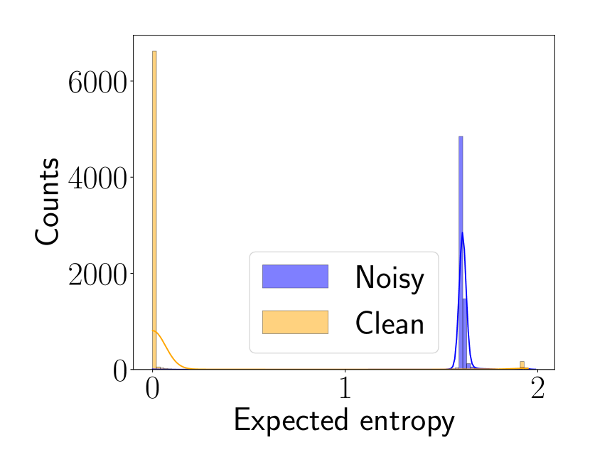
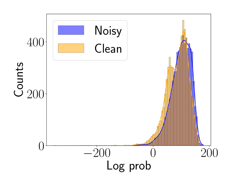
Figure 3: Left: The histogram depicts aleatoric uncertainty, represented as the expected entropy of the predictive distribution. It was computed using the formula specified in equation (4). Right: The histogram demonstrates epistemic uncertainty. It is computed using the logarithm of the density of the embeddings.

In the main discussions of this paper, we directly considered only two parts of our framework, resulting in a “switching” model, where one could abstain from the prediction of the local model and use the global model instead, or abstain from the prediction at all (if the certainty of global model is low).

In this part of the paper, we study another part of the pipeline – the ability to abstain from the prediction if aleatoric uncertainty (label noise or input ambiguity) is sufficiently big. Typical benchmark datasets like the ones we used are carefully curated and are found to have almost no label noise, as underscored by (Kapoor et al., 2022). Consequently, illustrating aleatoric uncertainty based solely on the information derived from these datasets can pose significant challenges.

Nevertheless, to facilitate the comprehensive execution of our proposed pipeline, we manually introduce artificial label noise. This strategic introduction serves a twofold purpose – not only does it effectively demonstrate our model’s capability to discern between aleatoric and epistemic uncertainties, but it also showcases that our model is unlikely to transition to a global model in the presence of high aleatoric uncertainty.

To conduct this examination, we change the labels of five classes – specifically, classes 5, 6, 7, 8, and 9 – within the MNIST dataset. The remainder of the classes, namely classes 0, 1, 2, 3, and 4, are retained in their original, unaltered state, thereby maintaining a degree of purity and control within our experiment.

The results of this experiment are presented in Figure 3. We see, that the aleatoric uncertainty, evaluated as an expected entropy of predictive distribution, drastically differs for noisy labels and for clean ones. Apparently, the threshold for the separation can be easily chosen using this histogram (e.g. the value of 1). Contrary to the measure of aleatoric uncertainty, the scores of epistemic uncertainty (here it is the logarithm of the density of features) can not distinguish between noisy and clean labels.

To conclude, the proposed framework effectively allows us to distinguish between noisy labels through the disentanglement of uncertainties into aleatoric and epistemic parts. This allows us to abstain from the prediction (when the label noise), or delegate inference to the global model (when input is out-of-distribution).

B.2 Computational overhead

One may worry that the introduction of the extra density model will make the approach prohibitively expensive. In fact, everything depends on the capacity of the chosen density model. Note, that in our case we are using one of the most simplest normalizing flows, namely Radial flow. For our experiments, we considered LeNet5 backbone (with 55k parameters), while the stack of normalizing flows (30 flows) had 5k parameters overall, so the computational overhead is very mild.

B.3 Separate tables for InD and OOD.

In this section, we represent Table 2 as two separate tables: Table 5 for benchmarking on InD data and Table 6 for benchmarking on OOD data. We clearly observe that FedPN shows superior results on OOD data while being competitive on in-distribution samples.

Dataset	FedAvg	FedRep	PerFedAvg	FedBabu	FedPer	FedBN	APFL	FedPN
MNIST	87.6	99.3	99.3	99.6	99.5	74.2	77.9	98.4
FashionMNIST	66.4	95.3	95.1	95.8	95.8	56.3	77.0	84.3
MedMNIST-A	58.1	96.9	96.2	97.3	97.7	47.8	98.0	96.2
MedMNIST-C	49.5	93.0	91.7	95.0	95.2	50.0	95.4	94.4
MedMNIST-S	38.9	87.4	86.7	90.5	90.9	40.5	91.8	86.9
CIFAR10	27.6	81.2	73.3	84.1	84.1	35.2	62.4	59.1
SVHN	80.6	94.7	93.4	94.9	95.4	74.4	80.5	87.1

Table 5: InD Data: Accuracy scores for in-distribution data. Values in bold are the best results.

Dataset	FedAvg	FedRep	PerFedAvg	FedBabu	FedPer	FedBN	APFL	FedPN
MNIST	82.3	0.0	50.0	61.8	29.4	65.0	58.9	98.3
FashionMNIST	55.2	0.0	22.9	22.4	15.2	51.8	34.0	78.2
MedMNIST-A	47.5	0.0	12.5	8.1	12.6	43.3	49.0	94.9
MedMNIST-C	45.5	0.0	2.4	13.6	10.9	43.3	53.3	88.7
MedMNIST-S	34.8	0.0	3.2	5.7	6.0	38.9	34.0	75.5
CIFAR10	23.3	0.0	0.0	1.4	0.6	28.6	15.0	28.8
SVHN	76.7	0.0	9.5	11.2	6.5	71.9	42.5	62.2

Table 6: OOD Data: Accuracy scores for out-of-distribution data. Values in bold are the best results.

B.4 Ablation Study for Threshold Selection

This experiment focuses on an ablation study of the selection of a threshold for switching between Local and Global models, based on the epistemic uncertainty of the Local model. We assessed the performance by measuring the accuracies of Local, Global, and Switch models on both InD and OOD data. We then calculated epistemic uncertainty scores, specifically the entropy of the predictive Dirichlet distribution (see Equation 3), on a calibration subset of the data. It’s important to note that this subset comes from the same distribution as the training data. The threshold selection, therefore, is a nuanced process in this context. Given the absence of explicit OOD data for more precise threshold tuning, we pretend that a portion of the calibration data is an OOD and select a corresponding quantile of epistemic uncertainty scores as our threshold.

The result of this experiment are shown in Figure 4. Here, the x-axis represents the quantile chosen for the threshold, while the y-axis displays the resulting accuracy.

We see that for some datasets, such as MNIST, the threshold selection is straightforward. The Switch model’s performance on InD and OOD aligns rapidly, and its accuracy is relatively insensitive to threshold variations.

In contrast, datasets like MedMNIST-A and FashionMNIST demand more careful threshold selection. Nevertheless, even for these datasets, a reasonable choice (e.g., quantile ($q\in[0.8,0.9]$, which correspond to $10-20$% of OOD in calibration data) yields satisfactory results.

Therefore, while threshold selection involves subjectivity, experiment shows that there is a "reasonable corridor" for threshold values that do not significantly compromise the accuracy of the resulting Switch model.

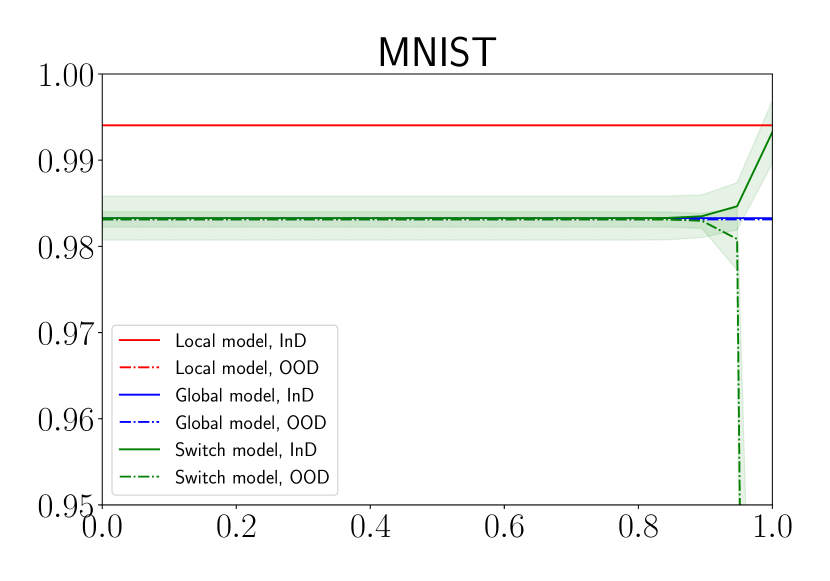
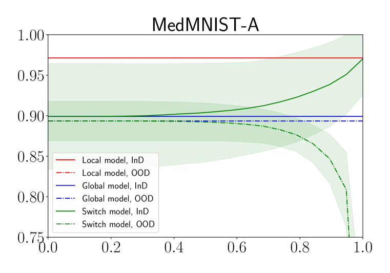
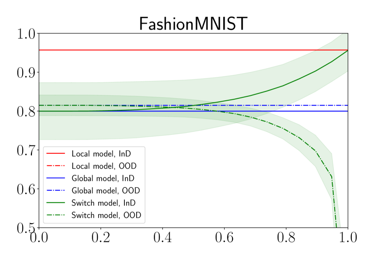
Figure 4: Performance comparison of Switch, Local, and Global models with varying switching thresholds. Note that the Local model’s accuracy is almost zero and does not appear within the considered range of y-axis values.

B.5 The Effect of Our StopGrad Modification

In this section, we conduct an empirical study to understand how our modified loss function impacts training under conditions of aleatoric uncertainty in the data. To simulate this, we introduce label noise into the MNIST dataset. Specifically, labels for half of the classes (5-9) are randomly swapped amongst themselves. We then set up a Federated Learning scenario with 20 clients, where each client has data from no more than three classes.

We initiate the federated training process using either our modified loss function (see Equation 8) or the standard Bayesian loss function (see Equation 6), keeping the number of training epochs consistent across both methods.

Figure 5 presents normalized histograms of the resulting $\log p(z)$ values for global models. This visualization reveals that when faced with aleatoric (label) noise, the model trained with the standard loss function tends not to assign significant probability mass to the noisy examples, even though these examples are part of its training distribution. In contrast, the model trained with our proposed loss function is incentivized to allocate probability mass to these examples. This outcome aligns with the expectation that $p(z)$ represents the density of training samples.

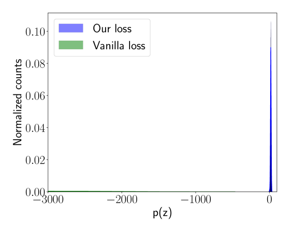
Figure 5: Normalized histogram of $\log p(z)$ for models trained with the standard Bayesian loss 6 and our modified loss 8.

References

- Arivazhagan et al. (2019) Manoj Ghuhan Arivazhagan, Vinay Aggarwal, Aaditya Kumar Singh, and Sunav Choudhary. Federated learning with personalization layers. arXiv preprint arXiv:1912.00818, 2019.
- Beluch et al. (2018) William H Beluch, Tim Genewein, Andreas Nürnberger, and Jan M Köhler. The power of ensembles for active learning in image classification. In Proceedings of the IEEE conference on computer vision and pattern recognition, pp. 9368–9377, 2018.
- Bengs et al. (2022) Viktor Bengs, Eyke Hüllermeier, and Willem Waegeman. Pitfalls of epistemic uncertainty quantification through loss minimisation. In Advances in Neural Information Processing Systems, 2022.
- Bengs et al. (2023) Viktor Bengs, Eyke Hüllermeier, and Willem Waegeman. On second-order scoring rules for epistemic uncertainty quantification. In Proceedings of the 40th International Conference on Machine Learning, volume 202, pp. 2078–2091. PMLR, 2023.
- Biloš et al. (2019) Marin Biloš, Bertrand Charpentier, and Stephan Günnemann. Uncertainty on asynchronous time event prediction. Advances in Neural Information Processing Systems, 32, 2019.
- Charpentier et al. (2020) Bertrand Charpentier, Daniel Zügner, and Stephan Günnemann. Posterior network: Uncertainty estimation without ood samples via density-based pseudo-counts. Advances in Neural Information Processing Systems, 33:1356–1367, 2020.
- Charpentier et al. (2022) Bertrand Charpentier, Oliver Borchert, Daniel Zügner, Simon Geisler, and Stephan Günnemann. Natural posterior network: Deep bayesian predictive uncertainty for exponential family distributions. In International Conference on Learning Representations, 2022.
- Charpentier et al. (2023) Bertrand Charpentier, Chenxiang Zhang, and Stephan Günnemann. Training, architecture, and prior for deterministic uncertainty methods. In ICLR 2023 Workshop on Pitfalls of limited data and computation for Trustworthy ML, 2023.
- Chen & Chao (2021) Hong-You Chen and Wei-Lun Chao. Fedbe: Making bayesian model ensemble applicable to federated learning. In ICLR, 2021.
- Collins et al. (2021) Liam Collins, Hamed Hassani, Aryan Mokhtari, and Sanjay Shakkottai. Exploiting shared representations for personalized federated learning. In ICML, pp. 2089–2099. PMLR, 2021.
- Deng et al. (2020) Yuyang Deng, Mohammad Mahdi Kamani, and Mehrdad Mahdavi. Adaptive personalized federated learning. arXiv preprint arXiv:2003.13461, 2020.
- Fallah et al. (2020) Alireza Fallah, Aryan Mokhtari, and Asuman Ozdaglar. Personalized federated learning with theoretical guarantees: A model-agnostic meta-learning approach. Advances in Neural Information Processing Systems, 33:3557–3568, 2020.
- Gal & Ghahramani (2016) Yarin Gal and Zoubin Ghahramani. Dropout as a bayesian approximation: Representing model uncertainty in deep learning. In International Conference on Machine Learning, pp. 1050–1059. PMLR, 2016.
- Graves (2011) Alex Graves. Practical variational inference for neural networks. Advances in neural information processing systems, 24, 2011.
- Hanzely & Richtárik (2020) Filip Hanzely and Peter Richtárik. Federated learning of a mixture of global and local models. arXiv preprint arXiv:2002.05516, 2020.
- He et al. (2016) Kaiming He, Xiangyu Zhang, Shaoqing Ren, and Jian Sun. Deep residual learning for image recognition. In Proceedings of the IEEE conference on computer vision and pattern recognition, pp. 770–778, 2016.
- Hüllermeier & Waegeman (2021) Eyke Hüllermeier and Willem Waegeman. Aleatoric and epistemic uncertainty in machine learning: An introduction to concepts and methods. Machine Learning, 110:457–506, 2021.
- Izmailov et al. (2021) Pavel Izmailov, Sharad Vikram, Matthew D Hoffman, and Andrew Gordon Gordon Wilson. What are bayesian neural network posteriors really like? In International conference on machine learning, pp. 4629–4640. PMLR, 2021.
- Kapoor et al. (2022) Sanyam Kapoor, Wesley J Maddox, Pavel Izmailov, and Andrew G Wilson. On uncertainty, tempering, and data augmentation in bayesian classification. Advances in Neural Information Processing Systems, 35:18211–18225, 2022.
- Kendall & Gal (2017) Alex Kendall and Yarin Gal. What uncertainties do we need in bayesian deep learning for computer vision? Advances in neural information processing systems, 30, 2017.
- Keswani et al. (2021) Vijay Keswani, Matthew Lease, and Krishnaram Kenthapadi. Towards unbiased and accurate deferral to multiple experts. In Proceedings of the 2021 AAAI/ACM Conference on AI, Ethics, and Society, pp. 154–165, 2021.
- Kim & Hospedales (2023) Minyoung Kim and Timothy Hospedales. Fedhb: Hierarchical bayesian federated learning. arXiv preprint arXiv:2305.04979, 2023.
- Kobyzev et al. (2020) Ivan Kobyzev, Simon JD Prince, and Marcus A Brubaker. Normalizing flows: An introduction and review of current methods. IEEE transactions on pattern analysis and machine intelligence, 43(11):3964–3979, 2020.
- Kotelevskii et al. (2022) Nikita Kotelevskii, Maxime Vono, Alain Durmus, and Eric Moulines. Fedpop: A bayesian approach for personalised federated learning. Advances in Neural Information Processing Systems, 35:8687–8701, 2022.
- Krizhevsky (2009) A Krizhevsky. Learning multiple layers of features from tiny images. Master’s thesis, University of Toronto, 2009.
- Lakshminarayanan et al. (2017) Balaji Lakshminarayanan, Alexander Pritzel, and Charles Blundell. Simple and scalable predictive uncertainty estimation using deep ensembles. Advances in neural information processing systems, 30, 2017.
- LeCun et al. (1998a) Yann LeCun, Léon Bottou, Yoshua Bengio, and Patrick Haffner. Gradient-based learning applied to document recognition. Proceedings of the IEEE, 86(11):2278–2324, 1998a.
- LeCun et al. (1998b) Yann LeCun, Corinna Cortes, and Christopher Burges. The mnist database of handwritten digits. http://yann. lecun. com/exdb/mnist/, 1998b.
- Lee et al. (2018) Kimin Lee, Kibok Lee, Honglak Lee, and Jinwoo Shin. A simple unified framework for detecting out-of-distribution samples and adversarial attacks. In Advances in Neural Information Processing Systems, volume 31, 2018.
- Li et al. (2021) Xiaoxiao Li, Meirui JIANG, Xiaofei Zhang, Michael Kamp, and Qi Dou. Fedbn: Federated learning on non-iid features via local batch normalization. In International Conference on Learning Representations, 2021.
- Liang et al. (2019) Paul Pu Liang, Terrance Liu, Liu Ziyin, Nicholas B Allen, Randy P Auerbach, David Brent, Ruslan Salakhutdinov, and Louis-Philippe Morency. Think locally, act globally: Federated learning with local and global representations. 2019.
- Linsner et al. (2022) Florian Linsner, Linara Adilova, Sina Däubener, Michael Kamp, and Asja Fischer. Approaches to uncertainty quantification in federated deep learning. In Machine Learning and Principles and Practice of Knowledge Discovery in Databases: International Workshops of ECML PKDD 2021, pp. 128–145, 2022.
- Malinin & Gales (2018) Andrey Malinin and Mark Gales. Predictive uncertainty estimation via prior networks. Advances in neural information processing systems, 31, 2018.
- Malinin & Gales (2019) Andrey Malinin and Mark Gales. Reverse kl-divergence training of prior networks: Improved uncertainty and adversarial robustness. Advances in Neural Information Processing Systems, 32, 2019.
- Malinin & Gales (2021) Andrey Malinin and Mark Gales. Uncertainty estimation in autoregressive structured prediction. In International Conference on Learning Representations, 2021.
- McMahan et al. (2017) Brendan McMahan, Eider Moore, Daniel Ramage, Seth Hampson, and Blaise Aguera y Arcas. Communication-efficient learning of deep networks from decentralized data. In Artificial intelligence and statistics, pp. 1273–1282. PMLR, 2017.
- Netzer et al. (2011) Yuval Netzer, Tao Wang, Adam Coates, Alessandro Bissacco, Bo Wu, and Andrew Y Ng. Reading digits in natural images with unsupervised feature learning. In NIPS Workshop on Deep Learning and Unsupervised Feature Learning, 2011.
- Oh et al. (2022) Jaehoon Oh, Sangmook Kim, and Se-Young Yun. Fedbabu: Towards enhanced representation for federated image classification. ICLR, 2022.
- Papamakarios et al. (2021) George Papamakarios, Eric T Nalisnick, Danilo Jimenez Rezende, Shakir Mohamed, and Balaji Lakshminarayanan. Normalizing flows for probabilistic modeling and inference. J. Mach. Learn. Res., 22(57):1–64, 2021.
- Rezende & Mohamed (2015) Danilo Rezende and Shakir Mohamed. Variational inference with normalizing flows. In International conference on machine learning, pp. 1530–1538. PMLR, 2015.
- Sensoy et al. (2018) Murat Sensoy, Lance Kaplan, and Melih Kandemir. Evidential deep learning to quantify classification uncertainty. Advances in neural information processing systems, 31, 2018.
- Xiao et al. (2017) Han Xiao, Kashif Rasul, and Roland Vollgraf. Fashion-mnist: a novel image dataset for benchmarking machine learning algorithms. arXiv preprint arXiv:1708.07747, 2017.
- Yang et al. (2021) Jiancheng Yang, Rui Shi, and Bingbing Ni. Medmnist classification decathlon: A lightweight automl benchmark for medical image analysis. In IEEE 18th International Symposium on Biomedical Imaging (ISBI), pp. 191–195, 2021.
- Yang et al. (2023) Jiancheng Yang, Rui Shi, Donglai Wei, Zequan Liu, Lin Zhao, Bilian Ke, Hanspeter Pfister, and Bingbing Ni. Medmnist v2-a large-scale lightweight benchmark for 2d and 3d biomedical image classification. Scientific Data, 10(1):41, 2023.