Generalised Adaptive Cross Approximation for Convolution Quadrature based Boundary Element Formulation

Abstract

The acoustic wave equation is solved in time domain with a boundary element formulation. The time discretisation is performed with the generalised convolution quadrature method and for the spatial approximation standard lowest order elements are used. Collocation and Galerkin methods are applied. In the interest of increasing the efficiency of the boundary element method, a low-rank approximation such as the adaptive cross approximation (ACA) is carried out. We discuss about a generalisation of the ACA to approximate a three-dimensional array of data, i.e., usual boundary element matrices at several complex frequencies. This method is used within the generalised convolution quadrature (CQ) method to obtain a real time domain formulation. The behaviour of the proposed method is studied with three examples, a unit cube, a unit cube with a reentrant corner, and a unit ball. The properties of the method are preserved in the data sparse representation and a significant reduction in storage is obtained.

Keywords: wave equation; boundary element method; generalised convolution quadrature; multivariate adaptive cross approximation

1 Introduction

Wave propagation problems appear often in engineering, e.g., for non-destructive testing or exploring the underground. Any of such problems are formulated with hyperbolic partial differential equations, e.g., in acoustics or elastodynamics. Sometimes the physical model allows to have a description with parabolic partial differential equations,e.g., for thermal problems. Despite that mostly a linear theory is sufficient, the handling of space and time requires expensive discretisation methods, where for scattering problems even an unbounded domain has to be considered.

Time domain boundary element methods (BEM) are a well established alternative to domain based methods like the finite element method, especially for scattering problems. The basis are boundary integral equations by the use of retarded potentials as counterpart to the governing hyperbolic partial differential equation. The mathematical theory goes back to the beginning of the last century by Fredholm for scalar problems like acoustics and later by Kupradze [16] for vectorial problems in elasticity. The mathematical background of time-dependent boundary integral equations is summarised by Costabel [10] and extensively discussed in the textbook by Sayas [30].

The first numerical realisation of a time domain boundary element formulation is originated by Mansur [23] in the 80th of the last century. Despite often used, this approach suffers from instabilities (see, e.g., [27]). A stable space-time formulation has been published by Bamberger and Ha-Duong [3], which has been further explored by the group of Aimi [1, 2]. These approaches work directly in time domain, whereas a transformation to Laplace- or Fourier-domain results in suitable formulations [11] as well. Somehow in between transformation and time domain methods are BE formulations based on the convolution quadrature (CQ) method proposed by Lubich [21, 22]. Such a formulation is a true time stepping method utilising the Laplace domain fundamental solutions and properties. Applications of the CQ to BEM can be found, e.g., in [31, 33]. The generalisation of this seminal technique to variable time step sizes has been proposed by López-Fernández and Sauter [18, 20] and is called generalised convolution quadrature method (gCQ). Applications can be found in acoustics with absorbing boundary conditions [29] and in thermoelasticity [17].

The drawback of all BE formulations either for elliptic and much stronger for hyperbolic problems is the high storage and computing time demand as a standard formulation scales with $\mathcal{O}(M^{2})$ for $M$ unknowns. In time domain, additionally, the time complexity has to be considered, where in the case of a CQ based formulation the complexity is of order $\mathcal{O}(M^{2}N)$ for $N$ time steps. For elliptic problems fast methods has been proposed as the fast multipole method (FMM) [15] or $\mathcal{H}$-matrix based methods with the adaptive cross approximation (ACA) used in the matrix blocks [8, 6]. For hyperbolic problems the extension of FMM to the time variable has been published in [14] for acoustics and in [36, 26] for elastodynamics. In combination with CQ, fast methods are published in combination with a reformulation of CQ. The CQ-algorithm can be rewritten such that several elliptic problems have to be solved [5, 32]. Based on this transformation the known techniques from the elliptic problems can be applied [4, 24].

Here, a different approach is used. Independently whether the CQ in the original form or gCQ is used, essentially, a three-dimensional data array has to be efficiently computed and stored. This data array is constructed by the spatial discretisation, resulting in two-dimensional data, and the used complex frequencies of the algorithm, which gives the third dimension. To find a low rank representation of this three-dimensional tensor the generalised adaptive cross approximation (3D-ACA) can be used. This technique is a generalisation of ACA [8] and is proposed by Bebendorf et al. [7, 9]. It is based on a Tucker decomposition [37] and can be traced back to the group of Tyrtyshnikov [25]. The 3D-ACA might be seen as a higher-order singular value decomposition or as a multilinear SVD [12], which is a generalisation of the matrix SVD to tensors. An alternative but related approach is presented in [13]. This approach does not look for a low rank representation but uses an interpolation with respect to the frequencies to reduce the total amount of necessary frequencies to establish the time domain solution.

Here, the 3D-ACA is applied on a gCQ based time domain formulation utilising the original idea of the multivariate ACA [9]. Recently a very similar approach has been published by Seibel [35], where the conventional convolution quadrature method is used and, contrary to the approach proposed here, the $\mathcal{H}^{2}$ technique is used for the approximation of the boundary element matrices at the different frequencies.

2 Problem statement

Let $\Omega\subset\mathbb{R}^{3}$ be a bounded Lipschitz domain and $\Gamma=\partial\Omega$ its boundary with the outward normal $\mathbf{n}$. The acoustic wave propagation is governed by

$$\frac{\partial^{2}}{\partial t^{2}}u(\mathbf{x},t)-c^{2}\Delta u(\mathbf{x},t) =0\quad (\mathbf{x},t) \in\Omega\times(0,T)$$ (1)

$$u(\mathbf{x},0)=\frac{\partial}{\partial t}u(\mathbf{x},0) =0\quad \mathbf{x} \in\Omega$$ (2)

$$\gamma_{0}u(\mathbf{x},t) =g_{D}(\mathbf{x},t)\quad (\mathbf{x},t) \in\Gamma_{D}\times(0,T)$$ (3)

$$\gamma_{1}u(\mathbf{x},t) =g_{N}(\mathbf{x},t)\quad (\mathbf{x},t) \in\Gamma_{N}\times(0,T)$$ (4)

with the wave speed $c$ and the end time $T>0$. $\Gamma_{D}$ and $\Gamma_{N}$ denote either a Dirichlet or Neuman boundary. The respective traces are defined by

$$\gamma_{0}u(\mathbf{x},t)=\lim_{\Omega\owns\mathbf{x}\to\mathbf{x}\in\Gamma}u(\mathbf{x},t)$$ (5)

for the Dirichlet trace and with

$$\gamma_{1,x}u(\mathbf{x},t)=\lim_{\Omega\owns\mathbf{x}\to\mathbf{x}\in\Gamma}\left(\nabla u(\mathbf{x},t)\cdot\mathbf{n}\right)=q(\mathbf{x},t)$$ (6)

for the Neumann trace, also known as the conormal derivative or flux $q(\mathbf{x},t)$.

The given problem can be solved with integral equations. Essentially, either an indirect approach using layer potentials or an direct approach are suitable. In the subsequent numerical tests both methodologies are used to show distinct features of the proposed method. First, the retarded boundary integral operators have to be formulated. It is the single layer potential

$$(\mathcal{V}*q)(\mathbf{x},t)=\int_{0}^{t}\int_{\Gamma}\gamma_{0}U(\mathbf{x}-\mathbf{y},t-\tau)q(\mathbf{y},\tau)\operatorname{d}s_{\mathbf{y}}\operatorname{d}\tau\;,$$ (7)

where the fundamental solution is are denoted by a capital letter $U(\mathbf{x}-\mathbf{y},t-\tau)$. The double layer potential is defined by

$$(\mathcal{K}*u)(\mathbf{x},t)=\int_{0}^{t}\int_{\Gamma}\gamma_{1,y}U(\mathbf{x}-\mathbf{y},t-\tau)u(\mathbf{y},\tau)\operatorname{d}s_{\mathbf{y}}\operatorname{d}\tau$$ (8)

and its adjoint

$$(\mathcal{K}^{\prime}*u)(\mathbf{x},t)=\int_{0}^{t}\gamma_{1,x}\int_{\Gamma}U(\mathbf{x}-\mathbf{y},t-\tau)u(\mathbf{y},\tau)\operatorname{d}s_{\mathbf{y}}\operatorname{d}\tau\;.$$ (9)

The remaining operator to be defined is the hypersingular operator

$$(\mathcal{D}*u)(\mathbf{x},t)=-\int_{0}^{t}\gamma_{1,x}\int_{\Gamma}\gamma_{1,y}U(\mathbf{x}-\mathbf{y},t-\tau)u(\mathbf{y},\tau)\operatorname{d}s_{\mathbf{y}}\operatorname{d}\tau\;.$$ (10)

Using these operators, which are also called retarded potentials, the solution for the Dirichlet problem related to (1) can be obtained by

$$\left(\mathcal{V}\ast q\right)\!\!\left(\mathbf{x},t\right)=\left(\mathcal{C}g_{D}+\left(\mathcal{K}\ast g_{D}\right)\right)\!\!\left(\mathbf{x},t\right)\quad(\mathbf{x},t)\in\Gamma_{D}\times(0,T)$$ (11)

with $\Gamma=\Gamma_{D}$. On the right hand side the so-called integral free term

$$\mathcal{C}g_{D}(\mathbf{x},t)=\lim_{\varepsilon\to 0}\int_{\partial B_{\varepsilon}(\mathbf{x})\cup\Omega}\nabla\frac{1}{\|\mathbf{x}-\mathbf{y}\|}\cdot\mathbf{n}\;g_{D}(\mathbf{y},t)\operatorname{d}s_{\mathbf{y}}+g_{D}(\mathbf{x},t)\;.$$ (12)

has to be considered with $B_{\varepsilon}(\mathbf{x})$ denoting a ball of radius $\varepsilon$ centered at $\mathbf{x}$ and $\partial B_{\varepsilon}(\mathbf{x})$ is its surface. In case of the Galerkin formulation this expression reduces to $1/2g_{D}(\mathbf{x},t)$ but in the collocation schema it is dependent on the geometry at the collocation node. Alternatively to (11), the indirect approach

$$(\mathcal{V}*\vartheta)(\mathbf{x},t)=g_{D}\!\left(\mathbf{x},t\right)\quad(\mathbf{x},t)\in\Gamma_{D}\times(0,T)$$ (13)

can be used, where $\vartheta(\mathbf{x},t)$ denotes the density function. The Neumann problem can be solved with the second boundary integral equation

$$\left(\mathcal{D}\ast u\right)\!\!\left(\mathbf{x},t\right)=-\left(\frac{1}{2}\mathcal{I}g_{N}-\left(\mathcal{K}^{\prime}\ast g_{N}\right)\right)\!\!\left(\mathbf{x},t\right)\quad(\mathbf{x},t)\in\Gamma_{N}\times(0,T)\;,$$ (14)

where the integral free term is already substituted by the expression holding only for the Galerkin approach.

3 Boundary element method: Discretisation

Spatial discretisation

The boundary $\Gamma$ is discretised with elements resulting in an approximation $\Gamma_{h}$ which is the union of geometrical elements

$$\Gamma_{h}=\bigcup_{e=1}^{E}\tau_{e}\,.$$ (15)

$\tau_{e}$ denote boundary elements, here linear surface triangles, and their total number is $E$.

Next, finite element bases on boundaries $\Gamma_{D}$ and $\Gamma_{N}$ are used to construct the approximation spaces

$$X_{D} =\operatorname{Span}\{\varphi_{1},\varphi_{2},\dots,\varphi_{M_{1}}\},$$ (16)

$$X_{N} =\operatorname{Span}\{\psi_{1},\psi_{2},\dots,\psi_{M_{2}}\}.$$ (17)

The unknowns $u$ and $q$ are approximated by a linear combination of functions in $X_{D}$ and $X_{N}$

$$u_{h}=\sum_{\ell=1}^{M_{1}}u_{\ell}(t)\varphi_{\ell}(\mathbf{x})\quad\text{and}\quad q_{h}=\sum_{k=1}^{M_{2}}q_{k}(t)\psi_{k}(\mathbf{x})\;.$$ (18)

Note, the coefficients $u_{\ell}(t)$ and $q_{k}(t)$ are still continuous functions of time $t$. In the following, the shape functions $\varphi_{i}$ will be chosen linear continuous and $\psi_{j}$ constant discontinuous. This is in accordance with the necessary function spaces for the integral equations, which are not discussed here (see [30]).

Inserting these spatial shape functions in the boundary integral equations (11) and applying the collocation method results in the semi-discrete equation system

$$\mathsf{V}\ast\mathsf{q}_{h}=\mathsf{C}\mathsf{g}_{D}+\mathsf{K}\ast\mathsf{g}_{D}$$ (19)

for the Dirichlet problem. The alternative solution is obtained by inserting the ansatz in (13) and applying the Galerkin schema

$$\mathsf{V}\ast\mathsf{\vartheta}_{h}=\mathsf{g}_{D}\;.$$ (20)

The Neumann problem is solved by (14) using these shape functions and the Galerkin method resulting in

$$\mathsf{D}\ast\mathsf{u}_{h}=-\frac{1}{2}\mathsf{g}_{N}+\mathsf{K}^{\prime}\ast\mathsf{g}_{N}\;.$$ (21)

The given boundary data are approximated by the same shape functions, respectively. The notation with sans serif fonts in (19), (20), and (21) indicates that in these vectors the nodal values are collected and in the matrices the respective values of the integrated fundamental solutions. In the Galerkin formulations double integrations have to be performed, whereas in the collocation schema only one spatial integration is necessary.

Temporal discretisation

Discretising the time in $N$ not necessarily constant time steps $\Delta t_{i}$, i.e.,

$$[0,T]=[0,t_{1},t_{2},\ldots,t_{N}],\quad\Delta t_{i}=t_{i}-t_{i-1},\;\;i=1,2,\ldots,N\,,$$

the generalized Convolution Quadrature Method (gCQ) [18, 20] can be applied. Let us assume an A- and L-stable Runge-Kutta method given by its Butcher tableau $\mathsf{c}$ $\mathsf{A}$ $\mathsf{b}^{\mathsf{T}}$ with $\mathsf{A}\in\mathbb{R}^{m\times m}$, $\mathsf{b},\mathsf{c}\in\mathbb{R}^{m}$ and $m$ is the number of stages. The stability assumptions require that $\mathsf{b}^{\mathsf{T}}\mathsf{A}^{-1}=(0,0,\ldots,1)$ holds. Exemplarily, the algorithm is shown for the indirect formulation. With the vector $\mathbbm{1}=(1,1,\ldots,1)^{\mathrm{T}}$ of size $m$ the semi-discretised integral formulation (20) can be approximated by

$$\mathsf{g}_{D}(t_{n})=\hat{\mathsf{V}}\left(\left(\Delta t_{n}\mathsf{A}\right)^{-1}\right)(\mathsf{\vartheta}_{h})_{n}+\sum\limits_{\ell=1}^{N_{Q}}\hat{\mathsf{V}}\left(s_{\ell}\right)\mathsf{W}^{\Delta t}_{\ell}\!\!\left((\mathsf{\vartheta}_{h})_{n-1}\right)\;.$$ (22)

The notation $()_{n}$ indicates the discrete value of the respective function/vector at $t_{n}$ and $\hat{\mathsf{V}}$ indicates that the Laplace transform of the integral kernel is used in the single layer operator. The whole algorithm can be given as in [19]

• First step

  $$\mathsf{g}_{D}\left(t_{1}\right)=\hat{\mathsf{V}}\left(\left(\Delta t_{1}\mathsf{A}\right)^{-1}\right)(\mathsf{\vartheta}_{h})_{1}$$

  with implicit assumption of zero initial condition.

• For all steps $n=2,\ldots,N$ the algorithm has two sub-steps

  1. Update the solution vector $\mathsf{x}_{n-1}$ at all integration points $s_{\ell}$

     $$\mathsf{x}_{n-1}\left(s_{\ell}\right)=\left(\mathsf{I}-\Delta t_{n-1}s_{\ell}\mathsf{A}\right)^{-1}\left(\left(\mathsf{b}^{\mathsf{T}}\mathsf{A}^{-1}\cdot\mathsf{x}_{n-2}(s_{\ell})\right)\mathbbm{1}+\Delta t_{n-1}\mathsf{A}(\mathsf{\vartheta}_{h})_{n-1}\right)$$ (23)

     for $\ell=1,\ldots,N_{Q}$ with the number of integration points $N_{Q}$.

  2. Compute the solution of the integral at the actual time step $t_{n}$

     $$\begin{split}\mathsf{g}_{D}\left(t_{n}\right)&=\hat{\mathsf{V}}\left(\left(\Delta t_{n}\mathsf{A}\right)^{-1}\right)(\mathsf{\vartheta}_{h})_{n}+\sum\limits_{\ell=1}^{N_{Q}}\omega_{\ell}\hat{\mathsf{V}}\left(s_{\ell}\right)\left(\mathsf{b}^{\mathsf{T}}\mathsf{A}^{-1}\cdot\mathsf{x}_{n-1}(s_{\ell})\right)\left(\mathsf{I}-\Delta t_{n}s_{\ell}\mathsf{A}\right)^{-1}\mathbbm{1}\\ &=\hat{\mathsf{V}}\left(\left(\Delta t_{n}\mathsf{A}\right)^{-1}\right)(\mathsf{\vartheta}_{h})_{n}+\sum\limits_{\ell=1}^{N_{Q}}\hat{\mathsf{V}}\left(s_{\ell}\right)\mathsf{W}^{\Delta t}_{\ell}\!\!\left((\mathsf{\vartheta}_{h})_{n-1}\right)\;.\end{split}$$ (24)

     The abbreviation $\mathsf{W}^{\Delta t}_{\ell}\!\!\left((\vartheta_{h})_{n-1}\right)=\omega_{\ell}\left(\mathsf{b}^{\mathsf{T}}\mathsf{A}^{-1}\cdot\mathsf{x}_{n-1}(s_{\ell})\right)\left(\mathsf{I}-\Delta t_{n}s_{\ell}\mathsf{A}\right)^{-1}\mathbbm{1}$ is introduced, where the dependency of $x_{n-1}$ on $(\mathsf{\vartheta}_{h})_{n-1}$ is implicitly denoted.

The parameters used above are given in A. Essentially, this algorithm requires the evaluation of the integral kernel at $N_{Q}$ points $s_{\ell}$, which are complex frequencies. Consequently, we get an array of system matrices. This array of system matrices can be interpreted as a three-dimensional array of data which will be approximated by a data-sparse representation based on 3D-ACA.

Before describing this algorithm, the discrete set of integral equations is given. For the Dirichlet problem, we have the direct approach

$$\hat{\mathsf{V}}\left(\left(\Delta t_{n}\mathsf{A}\right)^{-1}\right)(\mathsf{q}_{h})_{n}=\left(\mathsf{C}+\hat{\mathsf{K}}\left(\left(\Delta t_{n}\mathsf{A}\right)^{-1}\right)\right)(\mathsf{g}_{D})_{n}+\sum\limits_{\ell=1}^{N_{Q}}\left(\hat{\mathsf{K}}\left(s_{\ell}\right)\mathsf{W}^{\Delta t}_{\ell}\!\!\left((\mathsf{g}_{D})_{n-1}\right)-\hat{\mathsf{V}}\left(s_{\ell}\right)\mathsf{W}^{\Delta t}_{\ell}\!\!\left((\mathsf{q}_{h})_{n-1}\right)\right)$$ (25)

and the indirect approach

$$\hat{\mathsf{V}}\left(\left(\Delta t_{n}\mathsf{A}\right)^{-1}\right)(\mathsf{\vartheta}_{h})_{n}=(\mathsf{g}_{D})_{n}-\sum\limits_{\ell=1}^{N_{Q}}\hat{\mathsf{V}}\left(s_{\ell}\right)\mathsf{W}^{\Delta t}_{\ell}\!\!\left((\mathsf{\vartheta}_{h})_{n-1}\right)\;.$$ (26)

The Neuman problem is solved with the discrete equations

$$\begin{split}\hat{\mathsf{D}}&\left(\left(\Delta t_{n}\mathsf{A}\right)^{-1}\right)(\mathsf{u}_{h})_{n}=\\ &-\left(\frac{1}{2}\mathsf{I}-\hat{\mathsf{K}}^{\prime}\left(\left(\Delta t_{n}\mathsf{A}\right)^{-1}\right)\right)(\mathsf{g}_{N})_{n}+\sum\limits_{\ell=1}^{N_{Q}}\left(\hat{\mathsf{K}}^{\prime}\left(s_{\ell}\right)\mathsf{W}^{\Delta t}_{\ell}\!\!\left((\mathsf{g}_{N})_{n-1}\right)-\hat{\mathsf{D}}\left(s_{\ell}\right)\mathsf{W}^{\Delta t}_{\ell}\!\!\left((\mathsf{u}_{h})_{n-1}\right)\right)\;.\end{split}$$ (27)

4 Three-dimensional adaptive cross approximation

An approximation of a three-dimensional array of data or a tensor of third order $\mathcal{C}\in\mathbb{C}^{M\times M\times N_{Q}}$ in terms of a low-rank approximation has been proposed in [9] and is referred to as a generalisation of adaptive cross approximation or also called 3D-ACA. In this approach, the 3D array of data to be approximated is generated by defining the outer product by

$$\mathcal{C}=\mathbf{H}\otimes\mathbf{f}$$ (28)

with $\mathbf{H}\in\mathbb{C}^{M\times M},\ \mathbf{f}\in\mathbb{C}^{N_{Q}}$. The matrix $\mathbf{H}$ corresponds to the spatial discretization of the different potentials used in the boundary element formulations from above at a specific frequency $s_{\ell}$, e.g., the single layer potential in (26) on the right hand side. This matrix will be called face or slice and may be computed as a dense matrix or with a suitable hierarchical partition of the mesh as $\mathcal{H}$-matrix. Within this matrix different low-rank approximations can be applied. Here, the ACA [8] is used. Connected to this choice an hierarchical structure of the matrix has to be build with balanced cluster trees [6]. The vector $\mathbf{f}$, called fiber in the following, collects selected elements of $\mathbf{H}$ at the set of frequencies determined by the gCQ. The latter would amount in $N_{Q}$ entries and the same amount of faces. The 3D-ACA on the one hand approximates, as above mentioned, the faces with low rank matrices and, more importantly, the amount of necessary frequencies is adaptively determined. Hence, a sum of outer products $\mathcal{C}^{\ell}$ as given in (28) is established. The summation is stopped if $\mathcal{C}^{\ell}$ is comparable to $\mathcal{C}$ up to a prescribed precision $\varepsilon$. This is measured with a Frobenius-norm. The basic concept of this approach is sketched in Algorithm 1.

Algorithm 1 Pseudo code of 3D-ACA (taken from [35])

function 3D ACA($ENTRY,\varepsilon$) $\triangleright$ $ENTRY$ provides the integrated kernel values at collocation point $x_{i}$ and element $j$

     $\mathcal{C}^{(0)}=0,k_{1}=0$ and $\ell=0$

     while $\|\mathbf{H}_{\ell}\|_{F}\|\mathbf{f}_{\ell}\|_{2}>\varepsilon\|\mathcal{C}^{(\ell)}\|_{F}$ do

         $\ell=\ell+1$

         $H_{\ell}[i,j]=ENTRY(i,j,k_{\ell})-\mathcal{C}^{(\ell-1)}[i,j,k_{\ell}],\qquad i,j=1,\ldots,M$

         $H_{\ell}[i_{\ell},j_{\ell}]=\max_{i,j}|H_{\ell}[i,j]|$

         $f_{\ell}[k]=H_{\ell}[i_{\ell},j_{\ell}]^{-1}\left(ENTRY(i_{\ell},j_{\ell},k)-\mathcal{C}^{(\ell-1)}[i_{\ell},j_{\ell},k]\right),\qquad k=1,\ldots,N_{Q}$

         $\mathcal{C}^{(\ell)}=\mathcal{C}^{(\ell-1)}+\mathbf{H}_{\ell}\otimes\mathbf{f}_{\ell}$

         $k_{\ell+1}=\arg\max_{k}|f_{\ell}[k]|$

     end while

     $r=\ell-1$ $\triangleright$ Final rank, i.e., necessary frequencies return $\mathcal{C}^{r}=\sum\limits_{\ell=1}^{r}\mathbf{H}_{\ell}\otimes\mathbf{f}_{\ell}$

end function

Essentially, three-dimensional crosses are established. These crosses consist of a face $\mathbf{H}_{\ell}$, which is the respective matrix at a distinct frequency $s_{\ell}$ times a fiber $\mathbf{f}_{\ell}$, which contains one matrix entry, the pivot element, at all $N_{Q}$ frequencies. These crosses are added up until a predefined error is obtained. The amount of used frequencies is the so-called rank $r$ of this approximation of the initial data cube. The mentioned pivot element is denoted in Algorithm 1 with $H_{\ell}[i_{\ell},j_{\ell}]$. Like in the ’normal’ ACA this pivot element can be selected arbitrarily. However, selecting the maximum element ensures convergence. For details see [9] or the application using $\mathcal{H}^{2}$-matrices in the faces [35].

The stopping criterion requires a norm evaluation of $\mathcal{C}^{(\ell)}$. Assuming some monotonicity the norm can be computed recursively

$$\left\|\mathcal{C}^{(\ell)}\right\|_{F}^{2}=\sum\limits_{d,d^{\prime}}^{\ell}\left(\sum\limits_{i,j}H_{d}[i,j]\widebar{H_{d^{\prime}}[i,j]}\right)\left(\sum\limits_{k}f_{d}[k]\widebar{f_{d^{\prime}}[k]}\right)$$ (29)

following [35].

The multiplication of the three-dimensional data array with a vector is changed by the proposed algorithm. Essentially, the algorithm separates the frequency dependency such that $\mathbf{H}_{\ell}\left(\hat{\mathsf{V}}\right)$ is independent of the frequency and the fibers $\mathbf{f}_{\ell}\left(\hat{\mathsf{V}}\right)$ present this dependency. Let us use the multiplication on the right hand side of (26) as example. The multiplication is changed to

$$\sum\limits_{\ell=1}^{N_{Q}}\hat{\mathsf{V}}\left(s_{\ell}\right)\mathsf{W}^{\Delta t}_{\ell}=\sum\limits_{\ell=1}^{N_{Q}}\sum\limits_{\ell=1}^{r}\mathbf{H}_{\ell}\left(\hat{\mathsf{V}}\right)\otimes\mathbf{f}_{\ell}\left(\hat{\mathsf{V}}\right)\mathsf{W}^{\Delta t}_{\ell}=\sum\limits_{\ell=1}^{r}\mathbf{H}_{\ell}\left(\hat{\mathsf{V}}\right)\otimes\sum\limits_{\ell=1}^{N_{Q}}\mathbf{f}_{\ell}\left(\hat{\mathsf{V}}\right)\mathsf{W}^{\Delta t}_{\ell}\;.$$ (30)

The complexity of the original operation is $\mathcal{O}\left(N_{Q}M^{2}\right)$ for $M$ spatial unknowns. The approximated version has the complexity $\mathcal{O}\left(r(M^{2}+N_{Q})\right)$. It consists of the inner sum, which is a vector times vector multiplication of length $N_{Q}$, and the outer sum which is a matrix times vector multiplication of size $M$. Hence, the leading term with $M^{2}$ has only a factor of $r$ instead of $N_{Q}$ compared to the dense computation. It can be expected that for larger problem sizes with a significant reduction from $N_{Q}$ to $r$ complex frequencies this discrete convolution is faster.

Remarks for the implementation:

• There are two possibilities how to apply the 3D-ACA within the above given boundary element formulations. Either it can be applied on each matrix block, which requires that for the different frequencies the same hierarchical structure is used. This holds here as a pure geometrical admissibility criterium for the $\mathcal{H}$-matrix has been selected. The other choice would be to apply 3D-ACA on the $\mathcal{H}$-matrix as a whole. In the latter case the stopping criterion is determined by all matrix blocks, i.e., (29) is evaluated for each block and summed up. Consequently, the matrix block with the largest rank determines the overall rank. Hence, this choice results in a less efficient formulation as shown in [34]. Nevertheless, if the matrix structure in the different $\mathbf{H}_{\ell}$ differ this choice is a solution.

• In each face the ACA is used to compress these matrices beside the rank reduction with respect to the frequencies. Here, a recompression of the ACA is applied, which gives a representation of the admissible matrix blocks in a SVD like form $\mathcal{A}\approx\mathcal{A}_{r}=\mathbf{U}\Sigma\mathbf{V}^{H}$. Starting from the low rank representation of a block $\mathcal{A}_{r}=\mathbf{U}\mathbf{V}$, a QR-decomposition of the low-rank matrix $\mathbf{U}$ and $\mathbf{V}$ is performed

  $$\mathcal{A}\approx\mathcal{A}_{r}=\mathbf{U}\mathbf{V}^{H}=Q_{U}(R_{U}R_{V}^{H})Q_{V}^{H}=Q_{U}\,\check{\mathbf{U}}\check{\Sigma}\check{\mathbf{V}}^{H}Q_{V}^{H}=\overline{\mathbf{U}}\check{\Sigma}\overline{\mathbf{V}}^{H}$$ (31)

  and, secondly, the SVD is applied on the smaller inner matrix $R_{U}R_{V}^{H}$. The sketched technique improves the compression rates.

• Within the algorithm the largest element in a matrix block has to be found. For non-admissible blocks this operation requires to compare all block entries. For admissible blocks. the elements are not available directly and, hence, has either be computed out of the low-rank representation or an estimate can be used. Due to the recompression of the ACA-blocks low-rank matrices $\overline{\mathbf{U}}$ and $\overline{\mathbf{V}}$ consist of orthonormal columns and the estimation of the index $i$ of the pivot position can be found with

  $$\operatorname*{arg\,max}\limits_{i,j}\lvert a_{ij}\rvert=\operatorname*{arg\,max}\limits_{i,j}\sum_{k=1}^{r}\lvert u_{ik}\sigma_{k}\rvert\underbrace{\lvert v_{jk}\rvert}_{\leq 1}\leq\operatorname*{arg\,max}\limits_{i}\sum_{k=1}^{r}\lvert u_{ik}\sigma_{k}\rvert\;.$$ (32)

  The analogous way is used also for index $j$. This algorithm gives a pivot element which is approximately the largest element. However, in the computation of the fiber the original entries are used. Hence, the computation of the residuum is an approximation. For the single layer potential this approximation works fine but not for the double layer potential. In this case, the maximal element is determined by multiplying the low rank matrices, finding the largest element and deleting this dense block. Fortunately, such matrix operations can be efficiently implemented such that the computing time is not affected. Hence, in the presented results for all potentials this expanding to the dense matrix block is used.

5 Numerical examples

The above proposed method to accelerate the gCQ based time domain boundary element method is tested at three examples. First, a unit cube is used, second a cube with a reentrant corner (three-dimensional L-Shape), and third a unit ball. The first two test geometries are used for Dirichlet and Neumann problems, whereas in case of the unit ball only a Dirichlet problem is studied. For the latter case a non-smooth timely response of the solution has to be tackled. In all tests the main goal is to show that the approximation of the 3D-ACA does not spoil the results, i.e., the newly introduced approximation error is smaller than the error of the dense BE formulation. Main focus is on the overall obtained reduction in storage, i.e., the compression which is measured as the relation between the dense storage and the storage necessary for the proposed method.

To show that the 3D-ACA does not spoil the results the error in space in time is measured with

$$\begin{split}L_{max}(u_{h})&=\max\limits_{1\leq n\leq N}\|u\left(\frac{t_{n}+t_{n+1}}{2}\right)-u_{h}\left(\frac{t_{n}+t_{n+1}}{2}\right)\|_{L_{2}}\\ &=\max\limits_{1\leq n\leq N}\sqrt{\int\limits_{\Gamma}\left(u\left(\mathbf{x},\frac{t_{n}+t_{n-1}}{2}\right)-u_{h}\left(\mathbf{x},\frac{t_{n}+t_{n-1}}{2}\right)\right)^{2}\operatorname{d}\Gamma}\;,\end{split}$$ (33)

where $u$ and $u_{h}$ are placeholders for the presented quantity measured at the boundary of the selected domain $\Gamma$. This error is taken from [29] and measures the worst result in time and the usual spatial $L_{2}$-error. The convergence rate is denoted by

$$\mathrm{eoc}=\log_{2}\left(\frac{L_{max}^{h}}{L_{max}^{h+1}}\right)\;,$$ (34)

where the superscript $h$ and $h+1$ denotes two subsequent refinement level. The convergence results presented below does not change significantly if an $L_{2}$-error in time would be used as long as the time response is smooth. For the results of the sphere in the third subsection the drop in convergence is not that significant for an $L_{2}$-error in time as such a measure smears the error in time over all time steps.

As mentioned above, linear triangles are used for the discretisation of the geometry and either linear continuous or constant discontinuous shape functions for the unknown Cauchy data in the direct method are applied. In the indirect method constant discontinuous shape functions for the density are selected. The underlying time stepping method has been the 2-stage Radau IIA. The approximation within the faces has been chosen to be $\varepsilon_{ACA}=10^{-4}\ldots 10^{-8}$ for the different refinement levels of the spatial discretisation. In each refinement level the mesh size is halved as well as the time step size. The ratio of time steps to mesh size was kept constant with 0.7. The precision of the method with respect to the frequencies, i.e., the $\varepsilon$ in Algorithm 1 was selected as $\varepsilon=100*\varepsilon_{ACA}$. The final equation is solved with GMRES without any preconditioner, where the precision $\varepsilon_{ACA}$ is set. All results are computed for a wave speed $c=1\,\nicefrac{\mathrm{m}}{\mathrm{s}}$.

5.1 Example: Unit cube loaded by a smooth pulse

The first used test geometry is a unit cube $[-0.5,0.5]^{3}$ with the coordinate system located in the middle of the cube. In Fig. 1, this cube is displayed with the mesh of refinement level 3 and the table of all used meshes is given aside.

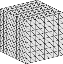
(a) Unit cube (level 3, $h=0.125\,\mathrm{m}$)

level	nodes	elements	$h$	$\Delta t$
1	50	96	0.5 m	0.3 s
2	194	384	0.25 m	0.15 s
3	770	1536	0.125 m	0.075 s
4	3074	6144	0.0625 m	0.0375 s
5	12290	24576	0.03125 m	0.01875 s

(b) Used meshes

Figure 1: Unit cube: Geometry and discretisation parameters

These meshes are created by bisecting the cathetus of the coarser mesh, starting with 8 elements on each face of the unit cube. As load a smooth pulse

$$u\left(\mathbf{y},t\right)=\frac{\left(t-\frac{r}{c}\right)^{2}}{r}e^{-c\left(t-\frac{r}{c}\right)}\;H\left(t-\frac{r}{c}\right)\qquad\text{with}\quad r=\|\mathbf{x}-\mathbf{y}\|$$ (35)

at the excitation point $\mathbf{x}=(0.8,0.2,0.3)^{\mathsf{T}}$ is used for the Dirichlet problem. For the Neumann problem the same geometry but with inverted normals, i.e., a cavity with the shape of the cube, is used. In this case the excitation point is at $\mathbf{x}=(0.3,-0.2,0.4)^{\mathsf{T}}$. The total observation time $T=3\,\mathrm{s}$ is selected such that the smooth pulse travels over the whole unit cube.

In the following, the results are discussed for a Dirichlet problem using (25) with a collocation approach and a Neumann problem using (27) with a Galerkin approach. In Fig. 2, the $L_{max}$-error defined in (33) is presented versus the different refinement levels, where ‘No Lwr’ means a computation applying the 3D-ACA but for the faces instead of the ACA dense matrix blocks are applied, i.e., the approximation is only with respect to the complex frequencies.

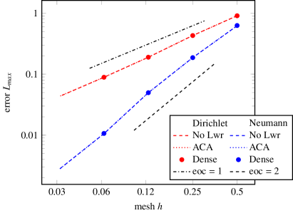
Figure 2: Cube: $L_{max}$-error versus refinement in space and time

The phrase ‘dense’ means no 3D-ACA at all and ‘ACA’ states that the algorithm from above is used with an ACA approximation also in the faces. Note, the refinement is done in space and time, i.e., not only $h$ is changed but as well $\Delta t$. The numbers displayed at this axis refer to the element size $h$. The expected oder of convergence is obtained considering that two factors influence the error. First, the spatial discretisation is expected to yield for a refinement in space a linear order for the constant shape functions used for the single layer potential, whereas the linear shape functions would result in a quadratic order for the hypersingular operator. These spatial known erros for the respective elliptic problem are combined with the 2-stage Radau IIA method used within the gCQ. This method would allow a third order convergence. However, as the spatial convergence orders are smaler they will dominate. This is clearly observed in Fig. 2. The second observation is that the 3D-ACA does not spoil the results. Certainly, the $\varepsilon$-parameters have to be adjusted carefully. As mentioned above, the ACA in the faces starts with $\varepsilon_{ACA}=10^{-4}$ in the coarsest level and is increased by $10^{-1}$ in each level up to $\varepsilon_{ACA}=10^{-8}$. The gCQ Algorithm 1 is terminated with $\varepsilon=100*\varepsilon_{ACA}$. Both parameters are found by trial and error.

After this check of a correct implementation and showing that the compression does not spoil the results, the efficiency with respect to the used frequencies, i.e., the rank in the third matrix dimension is studied. This gain of the 3D-ACA is presented in the Figs. 3 and 4 for the Dirichlet and Neumann problem, respectively. In both figures, the amount of used complex frequencies is given with respect to the mesh size, i.e., the refinement level.

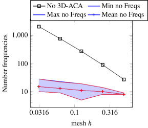
(a) Single layer potential

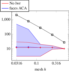
(b) Double layer potential

Figure 3: Cube: Number of used frequencies for the Dirichlet problem

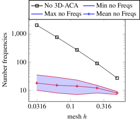
(a) Hyper singular operator

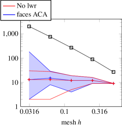
(b) Adjoint double layer potential

Figure 4: Cube: Number of used frequencies for the Neumann problem

Due to the selection of the different problems all of the four layer potentials from above are studied. Note, as the 3D-ACA is applied on the matrix blocks of the $\mathcal{H}$-matrix, each matrix block may have its own number of necessary complex frequencies. That is why a min-, max- and mean-value is given. Further, the numbers are displayed for the version using no approximation in the faces (red) and those with an ACA approximation within the faces (blue). Essentially, all operators show a drastic reduce of the used frequencies resulting in a drastic reduction of memory usage. Further, for more time steps (reducing time step size) only a very moderate increase in the number of frequencies is visible. Only for the double layer potentials the approximation with ACA significantly changes the maximum number of used frequencies, however not in the mean value. This is caused by the structure of the double layer potential, which includes on the one hand changing normal vectors resulting in blocks, which are badly approximated by ACA, and zero blocks. The zero blocks are not considered, however some frequencies are tested to make sure that the block under consideration is indeed a zero block. This results in the very low number of the min-value. The higher max values result from difficulties to determine the norm with (29) as the monotonicity is not that good in the above discussed blocks.

To display the adaptively selected frequencies, in Fig. 5 the complex frequencies of the gCQ are plotted in the complex plane exemplarily for level 4.

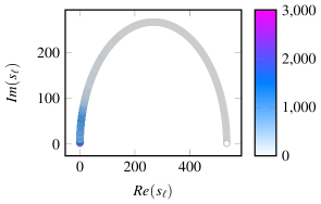
(a) Single layer potential

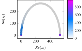
(b) Hyper singular operator

Figure 5: Cube (level 4): Used complex frequencies with a colour code for the number of matrix blocks, where this frequency is active

A dense formulation would use all frequencies. The colour code shows how much blocks in the 3D-ACA are evaluated at these frequencies. As the algorithm starts for all blocks with the first frequency selected by gCQ, this frequency is selected by all blocks (22432 for the single layer potential and 8560 for the hyper sigular operator). This number is deleted from the plot because else nothing would be visible due to the linear scaled colour range. The figure clearly shows that there is a region with small real parts where significant frequencies are detected by the algorithm. Surprisingly, the last complex frequency with large real part and nearly vanishing imaginary part is as well selected in case of the hypersingular operator. The same happens for the single layer potential, however for much less frequencies such that it is not visible in the plots above. For both double layer potentials similar pictures could be shown, where also for the adjoint double layer potential the last frequency is more often selected.

The above results indicate that the memory requirement of the proposed method is strongly improved compared to the standard formulation. As the right hand side is multiplied on the fly, i.e., the storage is the same for the new and the original formulation, the compression is only determined by the single layer and hypersingular operator in the Dirichlet and Neumann problem, respectively. This compression is plotted in Fig. 6 for both problems, Dirichlet and Neumann, versus the refinement.

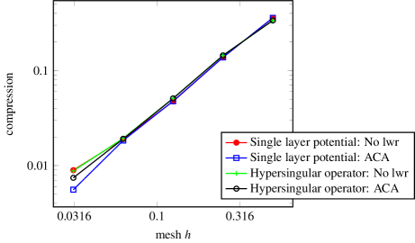
Figure 6: Cube: Compression of the data-sparse representation

As mentioned above, the compression is the relation between the required storage for the proposed formulation divided by the storage of a dense formulation. Obviously, the improvement is very strong, where the difference between the version without a compression in the face to the results with the ACA applied in the faces is not that strong. This is understandable if the sizes of the faces are considered. Those are not that large such that ACA can achieve a substantial improvement. Nevertheless, a compression of up to 0,56 % is a very good result.

Concerning the computing time a not that clear picture is possible. First, the complexity of the dense algorithm is $\mathcal{O}(N(\log(N))^{2}M^{2})$. This line is plotted in Fig. 7 as dotted line.

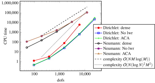
Figure 7: Cube: CPU time of the data-sparse representation

The dense Dirichlet problem follows this line, however, the Neumann problem not that clear. The reason might be the Galerkin formulation, which dominates the spatial matrix element calculation, and maybe avoids to be in the asymptotic range. The data sparse computations a clearly faster for the Dirichlet problem compared to the dense one but for the Neumann problem the advantage is not yet visible. Again it should be remarked that the Neumann problem uses a Galerkin method and the Dirichlet problem a collocation method. For the 3D-ACA the complexity line $\mathcal{O}(NM\log(M)$ seems to fit. However, it must be remarked that there is not any reason why this should hold. There is no indication in the algorithm that the adaptively determined rank $r$ is linear in $N$. Overall, it can be concluded that the 3D-ACA gives a very good performance with respect to the storage reduction but not that much savings in the CPU-time.

5.2 Example: Unit cube with reentrant corner (L-Shape) loaded by a smooth pulse

The next example is the same study as above but with a different geometry. The selected geometry is the three-dimensional version of an L-shape, i.e., a cube with a reentrant corner. The geometry as well as the parameters of the used meshes are given in Fig. 8.

(a) L-Shape (level 1, $h=0.5\,\mathrm{m}$)

level	nodes	elements	$h$	$\Delta t$
1	95	186	0.5 m	0.3 s
2	374	744	0.25 m	0.15 s
3	1490	2976	0.125 m	0.075 s
4	5954	11904	0.0625 m	0.0375 s
5	23810	47616	0.03125 m	0.01875 s

(b) Used meshes

Figure 8: L-Shape: Geometry and discretisation parameters

The total observation time $T=3\,\mathrm{s}$ is selected such that the smooth pulse travels over the whole computing domain. Note, the value $h$ in the table in Fig.  8 is misleading as it gives values of the largest elements, which are located on the not visible sides. Those elements on the side edges of the L-Shape on the left and right side have these sizes as well. Hence, towards the reentrant corner the mesh is refined compared to $h$. As above, a Dirichlet and a Neumann problem is studied. For both, the excitation point is selected in the reentrant part at $\mathbf{x}=(0.25,0.25,0.25)^{\mathsf{T}}$ and the load is the same smooth puls of (35). Note, the origin of the coordinate system is again in the center of the unit cube. Different to the setting above the Neumann problem is now not a scattering problem but computes the pressure at the surface of this L-Shape. The used equations are again (25) for the Dirichlet problem solved with a collocation approach and the Neumann problem uses (27) with a Galerkin approach.

First, as in the test above the convergence rates are reported to show that the proposed method keeps the error level of the dense computation. In Fig. 9, the $L_{max}$-error is plotted versus the refinement in space and time for the Dirichlet and Neumann problem.

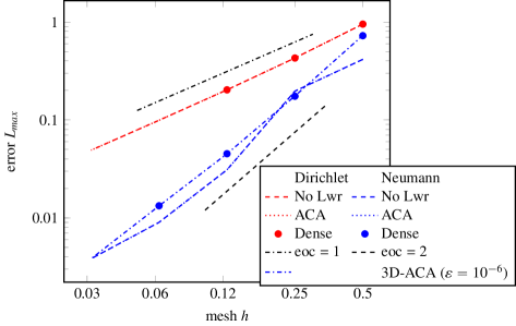
Figure 9: L-Shape: $L_{max}$-error versus refinement in space and time

In this figure three lines are visible. The Dirichlet problem is solved with the expected convergence rate and the dense computation gives the same results. For the Neumann problem the rate is still obtained also with the 3D-ACA but the error level is different. However, as indicated with the line ’3D-ACA ($\varepsilon=10^{-6}$)’ it is shown that for an increased precession the dense results can be recovered. This result confirms that the 3D-ACA has an influence on the computation and the $\varepsilon$-parameter must be carefully adjusted, despite that in this case the coarser approximation gives better results.

The used complex frequencies are as well studied for this geometry. They are displayed in Figs. 10 and 11.

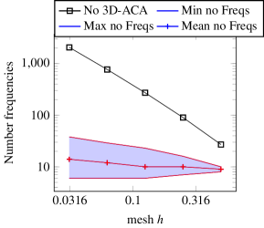
(a) Single layer potential

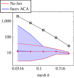
(b) Double layer potential

Figure 10: L-Shape: Number of used frequencies for the Dirichlet problem

Essentially, the pictures are similar to those for the unit cube and the numbers are comparable. Hence, there is no evidence that the geometry affects the used frequencies.

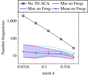
(a) Hyper singular operator

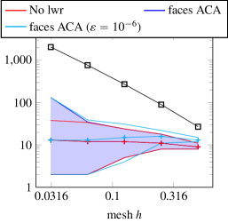
(b) Adjoint double layer potential

Figure 11: L-Shape: Number of used frequencies for the Neumann problem

Another remarkable point is the different numbers for an increased precession value $\varepsilon$. For the smaller meshes and less time steps the difference in the mean value is clearly visible but with increasing numbers for the times steps this difference vanishes. Hence, it may be concluded that the adaptivity inherently in the proposed algorithm detects the amount of frequencies necessary to give the physical behaviour of the solution. The compression rates are comparable to the unit cube and also the selection of the complex frequencies. Hence, these figures are skipped for the sake of brevity.

5.3 Example: Unit ball (sphere) loaded by a non-smooth pulse

The next example is used to show the influence of the time step size on the proposed method. The main feature of gCQ is to allow variable time step sizes to improve the approximation of solutions. Such gradings in time are necessary for non-smooth time behaviour of the solution. In the paper studying the numerical behaviour of the gCQ [19], a solution is selected where the behaviour in time is non-smooth such that a grading in the time mesh makes sense. This example is also used here to show the ability of the proposed approximation method to handle as well such solutions.

The selected geometry is a ball (sphere) with radius $1\,\mathrm{m}$. The geometry and the selected mesh are shown in Fig. 12.

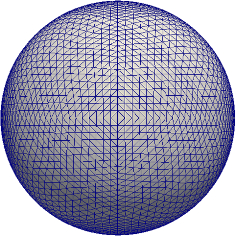
(a) Sphere with radius $1\,\mathrm{m}$

level	elements	$h$	$\Delta t_{const}$
1	7648	$\approx 0.05\,\mathrm{m}$	0.15 s
2	7648	$\approx 0.05\,\mathrm{m}$	0.075 s
3	7648	$\approx 0.05\,\mathrm{m}$	0.0375 s
4	7648	$\approx 0.05\,\mathrm{m}$	0.01875 s
5	7648	$\approx 0.05\,\mathrm{m}$	0.00938 s

(b) Used mesh and time step sizes

Figure 12: Sphere: Geometry, mesh size and used time step sizes

Different to the examples above, here, the spatial discretisation is not changed. This is motivated by the constructed solution. It is known that the density function within a single layer approach for the sphere corresponds to the spherical harmonics times the time derivative of the applied excitation in time [28]. Selecting the zeroth order spherical harmonic $Y_{0}^{0}\left(\mathbf{x}\right)$, the spatial solution is a constant function. This part of the solution is decoupled from the temporal solution, which might justify to keep the spatial discretisation constant and refine only in time. The selected excitation and analytical solution is

$$g_{D}\left(\mathbf{x},t\right)=Y_{0}^{0}\left(\mathbf{x}\right)t^{\frac{3}{2}}e^{-t}\quad\Rightarrow\quad\vartheta\left(\mathbf{x},t\right)=Y_{0}^{0}\left(\mathbf{x}\right)\sum\limits_{k=0}^{\lfloor t/2\rfloor}e^{-(t-2k)}\left(\frac{3}{2}\left(t-2k\right)^{\frac{1}{2}}-\left(t-2k\right)^{\frac{3}{2}}\right)\;.$$ (36)

The term with the square root shows a non-smooth behaviour in time starting at $t=0\,\mathrm{s}$ and is repeated in a periodic manner. Selecting the total observation time $T=1.5\,\mathrm{s}$ results in a solution, where the non-smooth part is only at the beginning. Hence, a graded time mesh

$$t_{n}=T\left(\frac{n}{N}\right)^{\alpha}=N\Delta t_{const}\left(\frac{n}{N}\right)^{\alpha}\qquad n=0,1,\ldots,N$$ (37)

can be recommended. The value $\Delta t_{const}$ is introduced to clarify the meaning of time step size, i.e., in Fig. 12 this value is listed. For $\alpha=2$ the full convergence order should be preserved. The effect of the grading can be observed in Fig. 13, where the $L_{max}$-error is presented versus a refinement in time for different exponents $\alpha$.

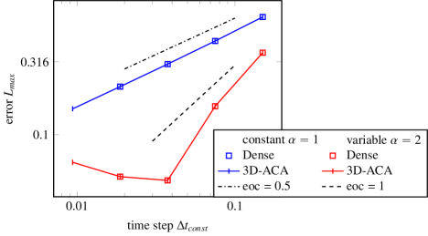
Figure 13: Sphere: $L_{max}$-error versus time step size for constant and variable time step size

The value $\alpha=1$ corresponds to a constant step size, where as expected the convergence order decreases to $\mathrm{eoc}=0.5$. With the graded mesh the convergence order is recovered. Note, the density function is approximated by constant shape functions, hence a order larger than 1 can not be expected. Obviously, there is a break in the convergence, where a further decrease of the time step size does not improve the result. This behaviour is already reported in [19] and reflects that the spatial discretisation is no longer suitable in combination with the spatial integration. Using the analytical solution in the spatial variable allows gCQ to keep the convergence order (see [19]). The proposed accelerated algorithm shows obviously the same behaviour. Hence, the approximation due to the 3D-ACA does not affect the efficiency of the gCQ based time domain BEM.

Next, the used complex frequencies are studied for this example. In Fig. 14 the amount of used complex frequencies is plotted for both temporal discretisations.

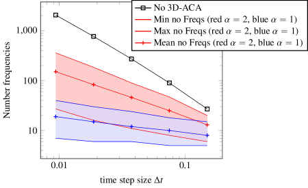
Figure 14: Sphere: Necessary frequencies for 3D-ACA where also the faces uses ACA

Obviously, the graded time mesh requires more frequencies compared to the constant discretisation. This holds true in the mean-value as well as in the max- and min-values. The tendency is as well that in this case the mean value does not approach a nearly constant amount of time steps. However, the increase is significantly smaler than in the dense method and very good compression can be obtained. The compression is for the first level 26% and in the fifth level 0,98 %. This reduction in storage is significant and allows to treat larger problems.

For this example it is interesting to report not only the numbers of used frequencies but also which frequencies are selected. In Fig. 15, the same plots as presented for the unit cube are shown.

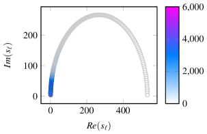
(a) $\alpha=1$

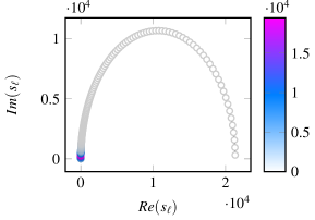
(b) $\alpha=2$

Figure 15: Sphere (level 3): Used complex frequencies with a colour code for the number of matrix blocks, where this frequency is active

First, looking at the right plot for the graded time mesh $\alpha=2$ it can be clearly seen how focused the frequencies are towards the imaginary axis and small real values. It is even visible that for large real values a coarsening happens. This is in accordance with the integration rule. The difference between the largest and smallest time step (parameter $q$ in A) determines the concentration of the frequencies towards the imaginary axis. Another effect independent of the 3D-ACA is the much larger values of the complex frequencies, i.e., the circle is larger. Please, have a look at the values on the axis compared to the left picture. Somehow as a consequence of this concentration as well the selected frequencies are concentrated towards small real values. It seems that the 3D-ACA preserves the properties of the integration rule.

6 Conclusions

Time domain boundary element formulations are usually very storage demanding as a lot of matrices for several time steps have to be stored. This is as well a significant drawback for the generalised convolution quadrature (gCQ) based formulation, where approximately $N\log N$ or more matrices each of the size of an elliptic problem have to be stored or more precise kept in memory. This reduces possible applications to very small sizes. The generalised adaptive cross approximation (3D-ACA) allows to find a low rank representations of three-dimensional tensors, hence this method is applied here to a gCQ based time domain BEM.

The results show a very significant reduction in storage while keeping the convergence of a dense computation. The algorithm is somehow a black-box technique as no modifications of the existing kernels of the dense formulation is necessary. The presented studies show the storage reduction for three different geometries, a unit cube, an L-shape, and a sphere. All three show similar behaviour with respect to the adaptively selected complex frequencies of the gCQ. The example with the sphere shows as well that the benefit of gCQ to select non-uniform time steps can be preserved, however for strongly different time step sizes the amount of necessary frequencies increases. Summarising, the application of 3D-ACA on the gCQ based time domain BEM gives a data sparse method with storage savings of more than 99%.

Acknowledgement

Financial support by the joint DFG/FWF Collaborative Research Centre CREATOR (CRC – TRR361/F90) is gratefully acknowledged.

Appendix A Parameters of the gCQ

The derivation and reasoning how the integration weights and points are determined can be found in [19, 20]. The result of these papers are recalled here. The integration points in the complex plane are

$$s_{\ell}=\gamma(\sigma_{\ell})\ , \omega_{\ell}=\frac{4K(k^{2})}{1\pi i}\gamma^{\prime}(\sigma_{\ell})\ , N_{Q}=N\log(N)\ ,$$

where for Runge-Kutta methods with $m>1$ stages it should be $N_{Q}=N\log^{2}(N)$. $K(k)$ is the complete elliptic integral of first kind

$$K(k)=\int^{1}_{0}\frac{dx}{\sqrt{(1-x^{2})(1-k^{2}x^{2})}}\ , K^{\prime}(k)=K(1-k)$$

and $K^{\prime}$ is its derivative, which equals the integral of the complementary modulus. The argument $k$ depends on the relation $q$ of the maximum and minimum step sizes in the following way

$$k=\frac{q-\sqrt{2q-1}}{q+\sqrt{2q-1}}\qquad q=5\frac{\Delta t_{\text{max}}\max_{i}|\lambda_{i}\left(\mathsf{A}\right)|}{\Delta t_{\text{min}}\min_{i}|\lambda_{i}\left(\mathsf{A}\right)|}\;,$$

with the eigenvalues $\lambda_{i}\left(\mathsf{A}\right)$. For the implicit Euler method the eigenvalues are 1 and the factor 5 in $q$ can be skipped. The functions $\gamma(\sigma_{\ell})$ and $\gamma^{\prime}(\sigma_{\ell})$ are

$$\gamma(\sigma_{\ell})= \frac{1}{\Delta t_{\text{min}}(q-1)}\left(\sqrt{2q-1}\frac{k^{-1}+\text{sn}(\sigma_{\ell})}{k^{-1}-\text{sn}(\sigma_{\ell})}-1\right)$$

$$\gamma^{\prime}(\sigma_{\ell})= \frac{\sqrt{2q-1}}{\Delta t_{\text{min}}(q-1)}\frac{2\ \text{cn}(\sigma_{\ell})\ \text{dn}(\sigma_{\ell})}{k(k^{-1}-\text{sn}(\sigma_{\ell}))^{2}}$$

$$\sigma_{\ell}= -K(k^{2})+\left(\ell-\frac{1}{2}\right)\frac{4K(k^{2})}{N_{Q}}+\frac{i}{2}K^{\prime}(k^{2})\,,$$

where $\text{sn}(\sigma_{\ell})$, $\text{cn}(\sigma_{\ell})$ and $\text{dn}(\sigma_{\ell})$ are the Jacobi elliptic functions. As seen from above, the integration contour is only determined by the largest and the smallest time steps chosen but not dependent on any intermediate step sizes. Due to the symmetric distribution of the integration points with respect to the real axis, only half of the frequencies $s_{\ell}$ need to be calculated.

Last, it may be remarked that for constant time steps $\Delta t_{i}=const$ the parameter determination would fail because this choice results in $q=1$ and $k=0$. Unfortunately, this value is not allowed for the complete elliptic integral. However, a slight change in the parameter $q\approx 1$ fixes this problem without spoiling the algorithm. The latter can be done as these parameter choices are empirical.

References

- Aimi and Diligenti [2008] A. Aimi and M. Diligenti. A new space-time energetic formulation for wave propagation analysis in layered media by BEMs. Int. J. Numer. Methods. Engrg., 75(9):1102–1132, 2008.
- Aimi et al. [2012] A. Aimi, M. Diligenti, A. Frangi, and C. Guardasoni. A stable 3d energetic Galerkin BEM approach for wave propagation interior problems. Eng. Anal. Bound. Elem., 36(12):1756–1765, 2012. ISSN 0955-7997. http://dx.doi.org/10.1016/j.enganabound.2012.06.003. URL http://www.sciencedirect.com/science/article/pii/S0955799712001361.
- Bamberger and Ha-Duong [1986] A. Bamberger and T. Ha-Duong. Formulation variationelle espace-temps pour le calcul par potentiel retardé d’une onde acoustique. Math. Meth. Appl. Sci., 8:405–435 and 598–608, 1986.
- Banjai and Kachanovska [2014] L. Banjai and M. Kachanovska. Fast convolution quadrature for the wave equation in three dimensions. J. Comput. Phys., 279:103–126, 2014. ISSN 0021-9991. https://doi.org/10.1016/j.jcp.2014.08.049. URL https://www.sciencedirect.com/science/article/pii/S0021999114006251.
- Banjai and Sauter [2008] L. Banjai and S. Sauter. Rapid solution of the wave equation in unbounded domains. SIAM J. Numer. Anal., 47(1):227–249, 2008.
- Bebendorf [2008] M. Bebendorf. Hierarchical Matrices: A Means to Efficiently Solve Elliptic Boundary Value Problems, volume 63 of Lecture Notes in Computational Science and Engineering. Springer-Verlag, 2008.
- Bebendorf [2011] M. Bebendorf. Adaptive cross approximation of multivariate functions. Constr. Approx., 34(2):149–179, 2011. 10.1007/s00365-010-9103-x. URL https://doi.org/10.1007/s00365-010-9103-x.
- Bebendorf and Rjasanow [2003] M. Bebendorf and S. Rjasanow. Adaptive low-rank approximation of collocation matrices. Computing, 70:1–24, 2003.
- Bebendorf et al. [2013] M. Bebendorf, A. Kühnemund, and S. Rjasanow. An equi-directional generalization of adaptive cross approximation for higher-order tensors. Appl. Num. Math., 74:1–16, 2013. ISSN 0168-9274. https://doi.org/10.1016/j.apnum.2013.08.001. URL http://www.sciencedirect.com/science/article/pii/S0168927413000950.
- Costabel [2005] M. Costabel. Time-dependent problems with the boundary integral equation method. In E. Stein, R. de Borst, and T. J. R. Hughes, editors, Encyclopedia of Computational Mechanics, volume 1, Fundamentals, chapter 25, pages 703–721. John Wiley & Sons, New York, Chichester, Weinheim, 2005.
- Cruse and Rizzo [1968] T. A. Cruse and F. J. Rizzo. A direct formulation and numerical solution of the general transient elastodynamic problem, I. Aust. J. Math. Anal. Appl., 22(1):244–259, 1968.
- De Lathauwer et al. [2000] Lieven De Lathauwer, Bart De Moor, and Joos Vandewalle. A multilinear singular value decomposition. SIAM J. Matrix Aanal. A., 21(4):1253–1278, 2000. 10.1137/S0895479896305696. URL https://doi.org/10.1137/S0895479896305696.
- Dirckx et al. [2022] Simon Dirckx, Daan Huybrechs, and Karl Meerbergen. Frequency extraction for bem matrices arising from the 3d scalar helmholtz equation. SIAM J. Sci. Comput., 44(5):B1282–B1311, 2022. 10.1137/20M1382957. URL https://doi.org/10.1137/20M1382957.
- Ergin et al. [1998] A. A. Ergin, B. Shanker, and E. Michielssen. Fast evaluation of three-dimensional transient wave fields using diagonal translation operators. J. Comput. Phys., 146(1):157–180, 1998. 10.1006/jcph.1998.5908.
- Greengard and Rokhlin [1997] L. Greengard and V. Rokhlin. A new version of the Fast Multipole Method for the Laplace equation in three dimensions. Acta Num., 6:229–269, 1997.
- Kupradze et al. [1979] V. D. Kupradze, T. G. Gegelia, M. O. Basheleishvili, and T. V. Burchuladze. Three-Dimensional Problems of the Mathematical Theory of Elasticity and Thermoelasticity, volume 25 of Applied Mathematics and Mechanics. North-Holland, Amsterdam New York Oxford, 1979.
- Leitner and Schanz [2021] Micael Leitner and Martin Schanz. Generalized convolution quadrature based boundary element method for uncoupled thermoelasticity. Mech Syst Signal Pr, 150:107234, 2021. ISSN 0888-3270. https://doi.org/10.1016/j.ymssp.2020.107234. URL http://www.sciencedirect.com/science/article/pii/S0888327020306208.
- Lopez-Fernandez and Sauter [2013] M. Lopez-Fernandez and S. Sauter. Generalized convolution quadrature with variable time stepping. IMA J. of Numer. Anal., 33(4):1156–1175, 2013. 10.1093/imanum/drs034.
- Lopez-Fernandez and Sauter [2015] M. Lopez-Fernandez and S. Sauter. Generalized convolution quadrature with variable time stepping. part II: Algorithm and numerical results. Appl. Num. Math., 94:88–105, 2015.
- López-Fernández and Sauter [2016] María López-Fernández and Stefan Sauter. Generalized convolution quadrature based on Runge-Kutta methods. Numer. Math., 133(4):743–779, 2016. 10.1007/s00211-015-0761-2.
- Lubich [1988a] C. Lubich. Convolution quadrature and discretized operational calculus. I. Numer. Math., 52(2):129–145, 1988a.
- Lubich [1988b] C. Lubich. Convolution quadrature and discretized operational calculus. II. Numer. Math., 52(4):413–425, 1988b.
- Mansur [1983] W. J. Mansur. A Time-Stepping Technique to Solve Wave Propagation Problems Using the Boundary Element Method. Phd thesis, University of Southampton, 1983.
- Messner and Schanz [2010] M. Messner and M. Schanz. An accelerated symmetric time-domain boundary element formulation for elasticity. Eng. Anal. Bound. Elem., 34(11):944–955, 2010. 10.1016/j.enganabound.2010.06.007.
- Oseledets et al. [2008] I. V. Oseledets, D. V. Savostianov, and E. E. Tyrtyshnikov. Tucker dimensionality reduction of three-dimensional arrays in linear time. SIAM J. Matrix Aanal. A., 30(3):939–956, 2008. 10.1137/060655894. URL https://doi.org/10.1137/060655894.
- Otani et al. [2007] Y. Otani, T. Takahashi, and N. Nishimura. A fast boundary integral equation method for elastodynamics in time domain and its parallelisation. In M. Schanz and O. Steinbach, editors, Boundary Element Analysis: Mathematical Aspects and Applications, volume 29 of Lecture Notes in Applied and Computational Mechanics, pages 161–185. Springer-Verlag, Berlin Heidelberg, 2007.
- Peirce and Siebrits [1997] A. Peirce and E. Siebrits. Stability analysis and design of time-stepping schemes for general elastodynamic boundary element models. Int. J. Numer. Methods. Engrg., 40(2):319–342, 1997. 10.1002/(SICI)1097-0207(19970130)40:2%3C319::AID-NME67%3E3.0.CO;2-I.
- Sauter and Veit [2013] S. Sauter and A. Veit. Retarded boundary integral equations on the sphere: Exact and numerical solution. IMA J. of Numer. Anal., 34(2):675–699, 2013.
- Sauter and Schanz [2017] S.A. Sauter and M. Schanz. Convolution quadrature for the wave equation with impedance boundary conditions. J. Comput. Phys., 334:442–459, 2017. ISSN 0021-9991. http://dx.doi.org/10.1016/j.jcp.2017.01.013. URL //www.sciencedirect.com/science/article/pii/S0021999117300232.
- Sayas [2016] F.-J. Sayas. Retarded Potentials and Time Domain Boundary Integral Equations: A Road Map, volume 50 of Springer Series in Computational Mathematics. Springer, Cham, 2016. 10.1007/978-3-319-26645-9.
- Schanz [2001] M. Schanz. Wave Propagation in Viscoelastic and Poroelastic Continua: A Boundary Element Approach, volume 2 of Lecture Notes in Applied Mechanics. Springer-Verlag, Berlin, Heidelberg, New York, 2001. 10.1007/978-3-540-44575-3.
- Schanz [2010] M. Schanz. On a reformulated convolution quadrature based boundary element method. CMES Comput. Model. Eng. Sci., 58(2):109–128, 2010. 10.3970/cmes.2010.058.109.
- Schanz and Antes [1997] M. Schanz and H. Antes. A new visco- and elastodynamic time domain boundary element formulation. Comput. Mech., 20(5):452–459, 1997. 10.1007/s004660050265.
- Schanz [2023] Martin Schanz. Realizations of the generalized adaptive cross approximation in an acoustic time domain boundary element method. Proc. Appl. Math. Mech., 23(2):e202300024, 2023. https://doi.org/10.1002/pamm.202300024. URL https://onlinelibrary.wiley.com/doi/abs/10.1002/pamm.202300024.
- Seibel [2022] Daniel Seibel. Boundary element methods for the wave equation based on hierarchical matrices and adaptive cross approximation. Numer. Math., 150(2):629–670, 2022. 10.1007/s00211-021-01259-8. URL https://doi.org/10.1007/s00211-021-01259-8.
- Takahashi et al. [2004] T. Takahashi, N. Nishimura, and S. Kobayashi. A fast BIEM for three-dimensional elastodynamics in time domain. Eng. Anal. Bound. Elem., 28(2):165–180, 2004. Erratum in EABEM, 28, 165–180, 2004.
- Tucker [1966] Ledyard R. Tucker. Some mathematical notes on three-mode factor analysis. Psychometrika, 31(3):279–311, 1966. 10.1007/BF02289464. URL https://doi.org/10.1007/BF02289464.