Axion-Mediated Inelastic Dark Matter

Abstract

We consider the axion-mediated scattering processes between dark matter (DM) and nucleon. The substantial contributions are made via the CP-odd gluonic current. Since the QCD axion is too feebly coupled to the visible particles, non-QCD axions are necessary to accomplish the relevant sensitivity from the current DM experiments. In the case of multi-component DM models, the inelastic scattering processes also make sizable contributions to the direct detection. The supersymmetry (SUSY) and clockwork (CW) mechanism provide a realistic model for the QCD axion and the axion-mediated DM scattering processes. In the SUSY CW axion model, the lightest axino is the DM particle and the axions mediate the elastic and inelastic scattering processes between the DM axino and nucleon. We show that the current and future XENONnT can produce relevant constraints for some parameter space of the model.

I Introduction

Dark matter (DM) is one of the most essential ingredients which form the current universe. In the early universe, DM develops the gravitational potential without generating the pressure, and consequently forms the structures much earlier than the case with only baryons. Its energy density is accurately measured by observing the cosmic microwave background (CMB) Planck:2018vyg , and large scale structure (LSS) eBOSS:2020yzd ; DES:2021wwk . While these measurements are firmly established via the gravitational interaction, no other interactions of DM are known and the identity of DM particles remains unanswered.

For a plausible explanation of the observed DM abundance, one may introduce weakly interacting massive particles (WIMPs) which are frozen out from the early universe due to their weak scale interactions with the visible particles, i. e., the standard model (SM) particles Jungman:1995df ; Bertone:2004pz . Among various ways to introduce weak-scale interactions, one lucrative scenario is that DM particles have neutral current interactions. DM species is one of electric neutral components of weak multiplets, so it has couplings of order the weak interaction. This scenario provides a good framework for the DM abundance, direct detection, and indirect detection without introducing new force carriers Goldberg:1983nd ; Ellis:1983wd ; Dienes:1998vg ; Cheng:2002iz ; Cirelli:2005uq . The Higgs portal is also an intriguing scenario which has a great discovery potential in diverse experiments Patt:2006fw . In other beyond-the-SM (BSM) models, DM interactions can be mediated by new gauge bosons Holdom:1985ag , and neutrinos Falkowski:2009yz .

In this article, we consider a new possibility that the DM scattering is mediated by the axions. The axion was originally introduced to solve the strong CP problem in the strong interaction. It is the pseudo-Nambu-Goldstone boson (pNGB) of the broken U(1) Peccei-Quinn symmetry, and automatically relaxes the QCD $\theta$ parameter to be zero Peccei:1977hh ; Weinberg:1977ma ; Wilczek:1977pj . The axion is indeed a good DM candidate. Its decay constant is of order the intermediate scale so that its lifetime is much larger than the age of the universe and the interactions are highly suppressed Kim:1979if ; Shifman:1979if ; Zhitnitsky:1980tq ; Dine:1981rt . Its coherent motion near the potential minimum can satisfy the observed DM density Abbott:1982af ; Preskill:1982cy ; Dine:1982ah ; Turner:1985si and produces unique features in the detection experiments Sikivie:1983ip . Since these features genuinely can also originate from the string landscape, a lot more axion-like particles arise in the high energy theory and they show a wide spectrum with various masses and decay constants Arvanitaki:2009fg . From now on, we use the term axion for all axion-like particles and the QCD axion is used only for axions whose mass is generated via the QCD confinement.

One can consider a new role of axions if DM couple to axions. The axions mediate the interaction between the DM particles and visible particles, so they can play a key role in the direct detection. The QCD axion is the simplest possibility because it is the necessary ingredient for resolving the strong CP problem. In this case, however, the interaction must be highly suppressed by the intermediate scale decay constant, and thus the axion cannot make any significant contribution to the DM direct detection. In this respect, axions with smaller decay constants (i. e., larger interactions) are required for substantially contributing the DM interactions.

A simple way is to introduce the axion with smaller decay constant regardless of its origin. Although there may be some constraints from the collider experiments Mimasu:2014nea ; Bauer:2017ris , flavor probes Bauer:2021mvw , beam dump experiments Dobrich:2015jyk and cosmology/astrophysics Depta:2020wmr ; Balazs:2022tjl , one can build a model where the axion mediation makes sizable contributions to the DM direct detection. In this paper, however, we consider a more systematic model which not only incorporates the axions and DM with sizable interactions but also involves the QCD axion.

The clockwork mechanism Choi:2014rja ; Choi:2015fiu ; Kaplan:2015fuy makes it possible to realize the QCD axion with the intermediate scale decay constant from $N\sim{\cal O}(10)$ pseudoscalar fields with the weak scale decay constants. The zero mode of the clockwork model becomes the QCD axion whose coupling is exponentially suppressed while the heavier modes keep their weak scale couplings Higaki:2015jag . Once the theory is supersymmetrized, moreover, it automatically includes the fermion partners of axions which we call axinos. The axinos indeed couple to the axions in the clockwork model, and they inherit the weak scale interactions from the axions. Therefore the lightest axino can be a good DM candidate and its scattering processes is mediated by a series of clockwork axions Bae:2020hys .

Furthermore, we have the same number of axino states and their mass difference can be small compared to their absolute mass scale. If this is the case, we can also see the inelastic scattering processes in the direct detection experiments Tucker-Smith:2001myb . In the detector, we will see the collective signature of various exited DM states and mediators.

This paper is organized as follows. In Sec. II, we consider a simple toy model which contain a non-QCD axion and a single-component Majorana fermion DM to illustrate how the axion-mediated process contributes to the DM-nucleon scattering. In Sec. III, we consider a 2-component DM model to argue the kinematics for the inelastic scattering process. In Sec. IV, we briefly review the SUSY CW axion model. In Sec. V, we present numerical analyses for the axino-mediated DM scattering including both the elastic and inelastic processes in the SUSY CW axion model. In Sec. VI, we conclude this paper.

II Axion-Mediated Process and Direct Detection

We can consider a simple model which contains an axion mediating the scattering process between the visible and DM sectors. The Lagrangian is given by

$${\cal L} = {\cal L}_{\rm kin}+\frac{1}{2}m_{\chi}\bar{\chi}\gamma^{5}\chi-V(a)$$ (1)

$$+\frac{g_{s}^{2}}{32\pi^{2}f}aG_{\mu\nu}^{b}\tilde{G}^{b\mu\nu}-\frac{\xi}{f}\left(\partial_{\mu}a\right)\bar{\chi}\gamma^{5}\gamma^{\mu}\chi$$

where ${\cal L}_{\rm kin}$ is the Lagrangian for kinetic terms, $\chi$ is the Majorana fermion DM, $m_{\chi}$ is the DM mass, $a$ is the axion, $G^{b}_{\mu\nu}$ and $\tilde{G}^{b}_{\mu\nu}$ are the gluon field strength and its dual, $g_{s}$ is the strong coupling constant, $f$ is the axion decay constant, and $\xi$ is the coupling constant. For the shift symmetry of the axion, we introduce only derivative interactions between the axion and DM fields. We consider the axion-gluon-gluon interaction for simplicity, but there can be the axion-photon-photon interaction. The axion potential is given by

$$V(a)=\Lambda^{4}\left[1-\cos\left(\frac{a}{f}\right)\right]$$ (2)

Here $\Lambda$ is the confinement scale of a QCD-like sector and should be larger than that of QCD, so we can avoid the strong constraints that apply to the QCD axion. The axion mass $m_{a}$ is thus $\sim\Lambda^{2}/f$ and can be a free parameter of the model.

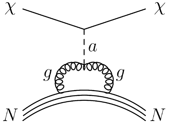
Figure 1: Feynman diagram for elastic scattering process

In this model, the gluon form factor substantially determines the DM-nucleon scattering process via the CP-odd gluonic current as shown in Fig. 1. The matrix element of the CP-odd gluonic current comes from the axion via the QCD chiral anomaly. In the large-$N_{c}$ and chiral limits, the form factor is expressed as Bishara:2017nnn

$$\langle N^{\prime}|\frac{\alpha_{s}}{8\pi}G^{b\mu\nu}\tilde{G}^{b}_{\mu\nu}|N\rangle = F^{N}_{\tilde{G}}(q^{2})\bar{u}^{\prime}_{N}i\gamma_{5}u_{N},$$ (3)

where $\bar{u}^{\prime}_{N}$ is the outgoing nucleon spinor, $u_{N}$ is the incoming nucleon spinor, and the momentum transfer is expressed by $q^{2}$. Taking into account the leading-order and next-to-leading-order terms, the form factor $F^{N}_{\tilde{G}}$ is given by

$$F^{N}_{\tilde{G}}(q^{2}) =-{m_{N}}\biggl{(} \frac{q^{2}}{m^{2}_{\pi}-q^{2}}a^{N}_{\tilde{G},\pi}+\frac{q^{2}}{m^{2}_{\eta}-q^{2}}a^{N}_{\tilde{G},\eta}$$ (4)

$$+b^{N}_{\tilde{G}}+c^{N}_{\tilde{G}}q^{2}+\mathcal{O}\left(q^{4}\right)\biggr{)},$$

where $m_{N}$ is the nucleon mass. The effective mass parameter and coupling constants are given by

$$\frac{1}{\tilde{m}} =\frac{1}{m_{u}}+\frac{1}{m_{d}}+\frac{1}{m_{s}},$$ (5)

$$a^{N}_{\tilde{G},\pi} \approx-\tilde{m}\frac{g_{A}}{2}\left(\frac{1}{m_{u}}-\frac{1}{m_{d}}\right),$$

$$a^{N}_{\tilde{G},\eta} \approx-\frac{\tilde{m}}{6}\left(\Delta u+\Delta d-2\Delta s\right)\left(\frac{1}{m_{u}}+\frac{1}{m_{d}}-\frac{2}{m_{s}}\right),$$

$$b^{N}_{\tilde{G}} \approx-\tilde{m}\left(\frac{\Delta u}{m_{u}}+\frac{\Delta d}{m_{d}}+\frac{\Delta s}{m_{s}}\right),$$

$$c^{N}_{\tilde{G}} \approx\left(\frac{1}{4\pi f_{\pi}}\right)^{2}.$$ (6)

Here $\Delta u=0.847,\Delta d=-0.407,\Delta s=-0.035,$ and $g_{A}=\Delta u-\Delta d=1.254$ FlavourLatticeAveragingGroup:2019iem . In the case for small momentum transfer, the dominant contribution comes from $b^{N}_{\tilde{G}}$.

The transition matrix element of the DM-nucleon scattering process is given by

$$\langle N^{\prime}\chi|\left(-i\frac{\xi}{f}\partial_{\mu}a\bar{\chi}\gamma^{\mu}\gamma^{5}{\chi}\right)\left(\frac{\alpha_{s}}{8\pi f}aG\tilde{G}\right)|N\chi\rangle$$ (7)

$$= -i\frac{\xi}{f^{2}}\langle N^{\prime}\chi|\left(\bar{\chi}\gamma^{\mu}\gamma^{5}{\chi}\right)\left(\partial_{\mu}a\right)a\frac{\alpha_{s}}{8\pi}G\tilde{G}|N\chi_{1}\rangle$$

$$= -\frac{\xi}{f^{2}}\frac{iq_{\mu}}{q^{2}-m^{2}_{a}}\langle\chi|\left(\bar{\chi}\gamma^{\mu}\gamma^{5}{\chi}\right)|\chi\rangle\langle N^{\prime}|\frac{\alpha_{s}}{8\pi}G\tilde{G}|N\rangle\,,$$

The matrix element is written with the form factor given in Eq. (3),

$$\mathcal{M}(\chi N\to\chi N^{\prime})= -\frac{1}{f^{2}}\frac{1}{q^{2}-m^{2}_{a}}\left(\bar{u}\not{q}\gamma_{5}u\right)$$

$$\times\left(\bar{u}^{\prime}_{N}i\gamma_{5}u_{N}\right)F_{\tilde{G}}(q^{2}).$$ (8)

where we have taken $\xi=1$ for simplicity. The spin-averaged square of matrix element is

$$|\overline{\mathcal{M}}|^{2} \simeq\left|\frac{1}{f^{2}}\frac{1}{q^{2}-m^{2}_{a}}\right|^{2}\left(4m^{2}_{\chi}q^{4}\right)F^{2}_{\tilde{G}}(q^{2})$$

$$\simeq\left|\frac{1}{f^{2}}\frac{1}{2m_{N}E_{R}+m^{2}_{a}}\right|^{2}\left(16m^{2}_{\chi}m^{2}_{N}E^{2}_{R}\right)F^{2}_{\tilde{G}}(E_{R}),$$ (9)

where we have used the approximate relation $q^{2}=E^{2}_{R}-2m_{N}E_{R}\simeq-2m_{N}E_{R}$, $E_{R}$ is the recoil energy and $m_{N}$ is the nucleon mass. In the lab frame, the differential cross section is expressed by

$$d\sigma = \frac{1}{2m_{N}2E_{\chi,i}v}\frac{d^{3}p_{N,f}}{(2\pi)^{3}E_{N,f}}\frac{d^{3}p_{\chi,f}}{(2\pi)^{3}E_{\chi,f}}$$ (10)

$$\times(2\pi)^{4}\delta^{4}(p_{\chi,i}+p_{N,i}-p_{\chi,f}-p_{N,f})\overline{|\mathcal{M}|^{2}}$$

$$=\frac{1}{64\pi^{2}m_{N}E_{\chi,i}v}\frac{|\vec{p}_{\chi,f}|}{E_{N,f}}d\Omega\overline{|\mathcal{M}|^{2}}$$

$$=\frac{|\vec{p}_{\chi,f}|}{64\pi^{2}m^{2}_{N}m_{\chi}v}d\Omega\overline{|\mathcal{M}|^{2}},$$

where initial (final) momenta and energy are denoted by $p_{i}(p_{f}),~{}E_{i}(E_{f})$, respectively. We have taken the approximation, $E_{\chi,i}\approx m_{\chi},~{}E_{N,f}\approx m_{N}$. The recoil energy is very small in the scattering process, so it is evaluated in the non-relativistic limit. The recoil energy is

$$E_{R} =\frac{|\vec{q}|^{2}}{2m_{N}}=\frac{|\vec{p}_{\chi,i}|^{2}+|\vec{p}_{\chi,f}|^{2}-2|\vec{p}_{\chi,i}||\vec{p}_{\chi,f}|\cos\theta}{2m_{N}}\,.$$ (11)

We can obtain

$$dE_{R} =-\frac{|\vec{p}_{\chi,i}||\vec{p}_{\chi,f}|}{m_{N}}d\cos\theta\rightarrow d\Omega=2\pi\frac{m_{N}}{|\vec{p}_{\chi,i}||\vec{p}_{\chi,f}|}dE_{R}.$$ (12)

Here we have used $d\Omega=-2\pi d\cos\theta$. Using Eqs. (10) and (12), we can construct the differential scattering cross section that reads Fan:2010gt ; Cirelli:2013ufw

$$\frac{d\sigma}{dE_{R}} =\frac{1}{32\pi m^{2}_{\chi}m_{N}v^{2}}\overline{|\mathcal{M}|^{2}}.$$ (13)

The differential cross section becomes

$$\frac{d\sigma}{dE_{R}} =\frac{E^{2}_{R}m_{N}}{2\pi f^{4}v^{2}}\left(\frac{1}{2m_{N}E_{R}+m^{2}_{a}}\right)^{2}F^{2}_{\tilde{G}}(E_{R}).$$ (14)

In the limit of the light mediator, $2m_{N}E_{R}\gg m^{2}_{a}$ , the differential cross section becomes

$$\frac{d\sigma}{dE_{R}} =\frac{1}{8\pi m_{N}f^{4}v^{2}}F^{2}_{\tilde{G}}(E_{R}).$$ (15)

In the limit of the heavy mediator corresponding to $q^{2}\to 0$, the differential cross section is

$$\frac{d\sigma}{dE_{R}} =\frac{E^{2}_{R}m_{N}}{2\pi f^{4}v^{2}m^{4}_{a}}F^{2}_{\tilde{G}}(E_{R}).$$ (16)

For a given recoil energy, the differential event rate for DM scattering off the xenon target in the unit of cpd (counts per day) per kilogram per keV, is then

$$\frac{dR}{dE_{R}} =\frac{\rho_{\chi}}{m_{\chi}}n_{T}A^{2}\int_{v_{\rm min}}^{v_{\rm esc}}vf(\vec{v})\frac{d\sigma}{dE_{R}}d^{3}v,$$ (17)

where $\rho_{\chi}=0.3$ ${\rm GeV/cm^{3}}$ is the local DM energy density, $n_{T}$ is the number density of the target atoms and $A$ represents the atomic number of the target material. The DM velocity in the galactic frame is described by the truncated Maxwell-Boltzmann distribution which corresponds to the isothermal sphere density profile:

$$f(\vec{v})d^{3}\vec{v} = \frac{N}{(v_{0}\sqrt{\pi})^{3}}e^{-v^{2}/v^{2}_{0}}d^{3}\vec{v},$$ (18)

where the most probable veolicty is given by $v_{0}=238$km/s v02016 ; Abuter:2021 , and the distribution is truncated at the escape velocity $v_{\rm esc}=544$ km/s v02016 . The normalization factor $N$ is

$$N = \frac{1}{{\rm erf}(v_{\rm esc}/v_{0})-\frac{2}{\sqrt{\pi}}(v_{\rm esc}/v_{0}){\rm exp}(-v^{2}_{esc}/v^{2}_{0})}.$$ (19)

to make the distribution satisfy the condition,

$$\int_{v\leq v_{\rm esc}}d^{3}vf(\vec{v})=1\,.$$ (20)

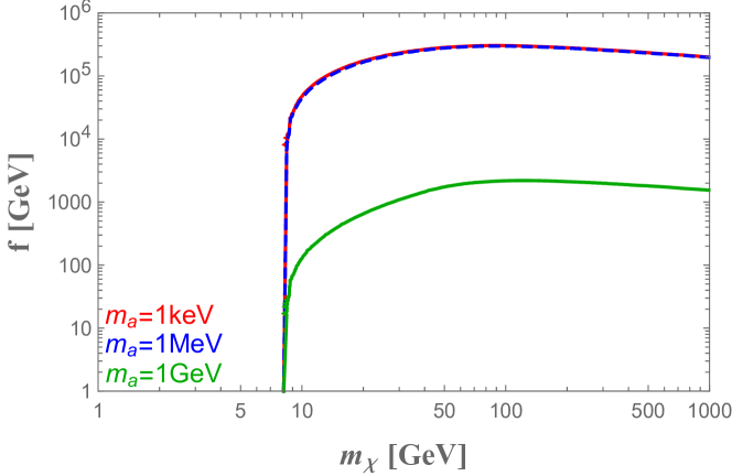
Figure 2: Direct detection bound for the model with the elastic scattering case is shown on $(m_{\chi},f)$-plane. Region below the lines are excluded by XENONnT. DM mass below $8$ GeV does not get any sensible bound due to the energy threshold.

The expected total event rate for DM (in)elastic scattering is

$$R = \int\epsilon(E_{R})\frac{dR}{dE_{R}}dE_{R}.$$ (21)

where $\epsilon(E_{R})$ is detector efficiency. For the recent result of XENONnT experiment, an energy range above 10% total efficiency lies between $3.3~{}{\rm keV_{NR}}$ to $60.5~{}{\rm keV_{NR}}$ and the amount of data is $1.1~{}\text{t}\cdot\text{yr}$. Assuming only the statistical uncertainties, the 90% confidence level sensitivity is 2.3 events if there is a null DM scattering event. We analyze the XENONnT bound on $(m_{\chi},f)$-plane for the simple model in Eq. 1. In Fig. 2, We show the XENONnT bound for three benchmark points with $m_{a}=1$ keV, $1$ MeV, and $1$ GeV. For a small $m_{a}$, the cross section is nearly independent of the axion mass and consequently the explicit $E_{R}$ dependence is cancelled out, XENONnT results have a rather strong sensitivity up to $f\sim 10$ TeV region. For a larger $m_{a}$, the cross section gets suppressed by the factor $E_{R}^{2}m_{N}^{2}/m_{a}^{4}$, so the sensitivity is weaker than the small mass cases.

III Multi-Component DM Model and Inelastic Processes

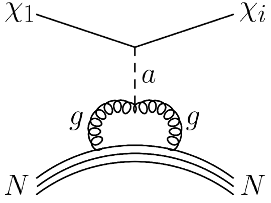
Figure 3: Feynman diagram for both elastic and inelastic scattering process

We elevate the axion-mediated DM model to a multi-component DM model in order to elucidate the impact of inelastic processes. The Lagrangian includes the interactions which involve different DM component:

$${\cal L} = {\cal L}_{\rm kin}+\frac{1}{2}m_{\chi_{i}}\bar{\chi_{i}}\gamma^{5}\chi_{i}-V(a)$$ (22)

$$+\frac{g_{s}^{2}}{32\pi^{2}f_{a}}aG_{\mu\nu}^{b}\tilde{G}^{b\mu\nu}-\frac{\xi_{ij}}{f_{a}}\left(\partial_{\mu}a\right)\bar{\chi_{i}}\gamma^{5}\gamma^{\mu}\chi_{j}\,.$$

Here the DM masses are assumed to be diagonal while the coupling constant, $\xi_{ij}$ contains both diagonal and non-diagonal components. The lightest component contributes to the dominant DM abundance, so is the initial state of the DM-nucleon scattering process. The final state of the process, however, can be any component of $\chi_{i}$. Therefore both the elastic and inelastic processes contribute to the DM-nucleon scattering as shown in Fig.  3.

Let us consider a simple 2-component case where $\xi_{11}=\xi_{22}=\xi_{12}=\xi$. We assume that $\chi_{1}$ is the dominant DM in the universe, while $\chi_{2}$ is slightly heavier than $\chi_{1}$. In this case, a sizable contribution to the DM detection is also made by the inelastic process, $\chi_{1}N\to\chi_{2}N^{\prime}$ if the DM particle has enough energy. In the non-relativistic limit, the recoil energy of the scattering process is given by Bramante:2016rdh

$$E_{R}=\frac{\mu}{m_{T}} \left[\mu v^{2}\cos^{2}\theta-\delta\right.$$

$$\left.\pm\sqrt{\mu v^{2}\cos^{2}\theta}\sqrt{\mu v^{2}\cos^{2}\theta-2\delta}\right],$$ (23)

where $m_{T}$ is the target nuclear mass, $\mu$ is the reduced mass between dark matter and target nucleus, $\theta$ is the scattering angle in the lab frame, and $\delta=m_{\chi_{2}}-m_{\chi_{1}}$. In this expression, we can see both the lower and upper bound on the recoil energy.

The smallest value for the required DM velocity is given by

$$v_{\rm min}=\frac{1}{\sqrt{2E_{R}m_{T}}}\left(\frac{E_{R}m_{T}}{\mu}+\delta\right)\,,$$ (24)

and the recoil energy for $v_{\rm min}$ is given by

$$E_{R}(v_{\rm min})\simeq\begin{cases}\delta&(\text{for}~{}~{}m_{\chi}\gg m_{T})\,,\\ \frac{m_{\chi}}{m_{T}}\delta&(\text{for}~{}~{}m_{\chi}\ll m_{T})\,.\end{cases}$$ (25)

In Fig. 4, we show the available recoil energies on a xenon target depending on $\delta$ for $m_{\rm DM}=100$ GeV. The available recoil energy region for XENONnT experiment is between horizontal lines. The vertical line corresponds to the escape velocity of DM in our galaxy. We can see that the phase space of the inelastic scattering shrinks and thus the event rate decreases as $\delta$ increases. When $\delta$ is larger than $90$ keV, the phase space of the inelastic scattering is closed and only the elastic scattering process are involved.

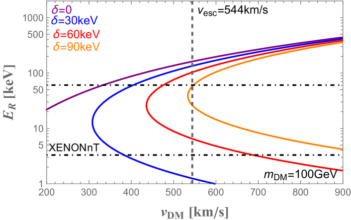
Figure 4: The available range of recoil energies on a nuclear target, for a given DM mass. The dot-dashed black horizontal lines indicate the minimum and maximum recoil energy windows used by XENONnT collaboration XENON:2023cxc . The gray vertical line is the DM escape velocity.

From the Lagrangian in Eq. (22) and the matrix element for the single component case in Eq. (8), we can easily evaluate the matrix element for both the elastic and inelastic DM-nucleon scattering processes:

$$\mathcal{M}(\chi_{1}N\to\chi_{i}N^{\prime}) =\frac{1}{f^{2}}\frac{1}{q^{2}-m^{2}_{a}}\left(\bar{u}_{i}\gamma_{5}\not{q}u_{1}\right)$$

$$\times\left(\bar{u}^{\prime}_{N}i\gamma_{5}u_{N}\right)F_{\tilde{G}}(q^{2}).$$ (26)

where $i=1,2$ and we have set $\xi=1$. Similarly, the spin-averaged square of matrix element is given by

$$|\overline{\mathcal{M}(\chi_{1}N\to\chi_{i}N^{\prime})}|^{2}\simeq \left|\frac{1}{f_{a}^{2}}\frac{1}{q^{2}-m^{2}_{a}}\right|^{2}\left(4m^{2}_{\chi_{1}}q^{4}\right)F^{2}_{\tilde{G}}(q^{2})$$

$$+\mathcal{O}(\delta_{i})\,.$$ (27)

where $\delta_{1}=0$ and $\delta_{2}=\delta$. It is worth stressing that the squared matrix element has the terms of ${\cal O}(\delta)$ in the inelastic process while the elastic case remains the same form as in Eq. (9). In the observable parameter space for the inelastic scattering process, $\delta$-dependent term is small enough to be safely neglected. Therefore we can use the same expression of the squared matrix element shown in Eq. (9) for both processes. The $\delta$-dependence, on the other hand, still exists implicitly in $E_{R}$ and $v_{\rm min}$ in the final event rate caculation.

Similarly to that of the simple model in Eq. (14), the differential cross section becomes

$$\frac{d\sigma_{i}}{dE_{R}}\equiv \frac{d\sigma}{dE_{R}}(\chi_{1}N\to\chi_{i}N^{\prime})$$

$$= \frac{E^{2}_{R}m_{N}}{2\pi f_{a}^{4}v^{2}}\left(\frac{1}{2m_{N}E_{R}+m^{2}_{a}}\right)^{2}F^{2}_{\tilde{G}}(E_{R}).$$ (28)

The differential event rate is also given by the same expression:

$$\frac{dR_{i}}{dE_{R}} =\frac{\rho_{\chi_{1}}}{m_{\chi_{1}}}n_{T}A^{2}\int_{v_{\rm min}}^{v_{\rm esc}}vf(\vec{v})\frac{d\sigma_{i}}{dE_{R}}d^{3}v,$$ (29)

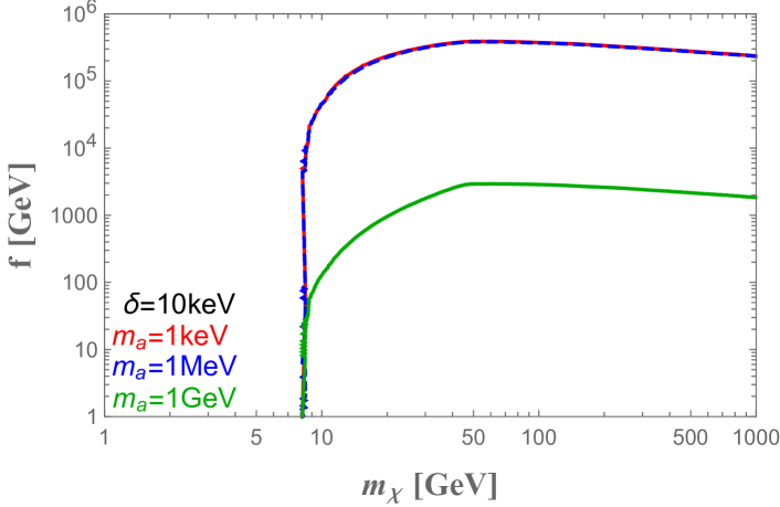
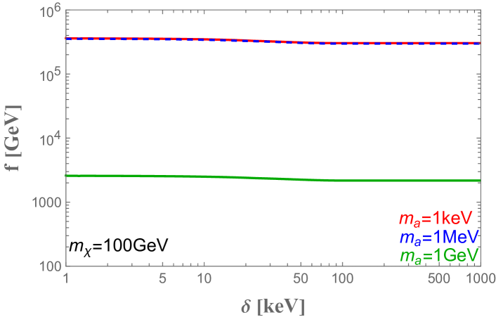
Figure 5: The XENONnT bound for the 2-component model is shown on $(m_{\chi},f)$-plane in the upper panel and in $(\delta,f)$-plane in the lower panel. Due to the energy threshold, DM mass below $8$ GeV is not constrained.

The expected total event rate for DM is the sum of the elastic and inelastic processes:

$$R=\sum_{i=1}^{2}\int\epsilon(E_{R})\frac{dR_{i}}{dE_{R}}dE_{R}\,.$$ (30)

Each process implicitly depends on the mass difference $\delta$ in the $E_{R}$ and $v_{\rm min}$ in Eqs. (29) and (30), although the explicit $\delta$ dependence is neglected in the squared matrix element in Eq. (27).

In Fig. 5, we show the XENONnT bound for the 2-component model. The bound is similar to the single component model because the elastic and inelastic process are similar in the cross section.

IV Supersymmetric Clockwork Axion Model

IV.1 Supersymmetric Clockwork Mechanism

In this section, we briefly present the supersymmetric (SUSY) clockwork (CW) axion model and its dark matter sector as a well-motivated and well-organized model for axion-mediated dark matter which contains many fermion states in the dark sector. We follow the basic construction in Ref. Bae:2020hys which utilizes a simple formulation in Ref. Kaplan:2015fuy ; Giudice:2016yja for realizing the CW structure. The model consists of $N+1$ superfield $\Phi_{j}$ containing the pseudo-Nambu-Goldstone Bosons (pNGBs) and their SUSY partners:

$$\Phi_{j}=\frac{1}{\sqrt{2}}(\sigma_{j}+i\phi_{j})+\sqrt{2}\theta\psi_{j}+\theta^{2}F_{j}$$ (31)

where $\sigma_{j}$, $\phi_{j}$ and $\psi_{j}$ are the scalar, pseudoscalar and fermion components of the superfield. The pseudoscalar $\phi_{j}$’s correspond to the pNGBs reflecting the shift symmetries originating from the spontaneously broken global U(1) symmetries.

The effective Kähler potential and superpotential are given by

$$K_{\rm eff} = v_{0}^{2}\sum_{j=0}^{N}\left[\cosh\left(\frac{\Phi_{j}+\Phi_{j}^{\dagger}}{v_{0}}\right)\right.$$ (32)

$$\left.+\xi\sinh\left(\frac{\Phi_{j}+\Phi_{j}^{\dagger}}{v_{0}}\right)\right]\,,$$

$$W_{\rm eff} = m_{\Phi}v_{0}^{2}\sum_{j=0}^{N-1}\cosh\left(\frac{\Phi_{j}-q\Phi_{j+1}}{v_{0}}\right)\,,$$ (33)

where $v_{0}$ is the mass scale for the U(1) symmetry breaking, $\xi$ is a dimensionless parameter, $m_{\Phi}$ is a mass parameter, and $q$ is a constant of order unity. In the limit of $m_{\Phi}\to 0$, the theory is invariant under the field transformation

$$\phi_{j}\to\phi_{j}+\beta_{j}$$ (34)

where $\beta_{j}$’s are arbitrary real numbers. Thus the $N+1$ shift symmetries are manifestly preserved. For $m_{\Phi}\neq 0$, $N$ shift symmetries become broken leaving one shift symmetry corresponding to

$$\phi_{j}\to\phi_{j}+\beta/q^{j}\,,$$ (35)

where $\beta$ is an arbitrary real number. This feature is clearly shown when the superpotential is expanded to the quadratic order:

$$W_{\rm eff} = \frac{1}{2}m_{\Phi}v_{0}^{2}\sum_{j=0}^{N-1}\left(\frac{\Phi_{j}-q\Phi_{j+1}}{v_{0}}\right)^{2}+\cdots$$ (36)

$$= \frac{1}{2}m_{\Phi}\sum_{j,k=0}^{N}{\bf M}_{\text{CW}jk}\Phi_{j}\Phi_{k}+\cdots\,,$$

where we have dropped the constant term. The CW matrix $\bf M_{\rm CW}$ is given by

$${\mathbf{M}}_{\rm CW}=\begin{pmatrix}1&-q&0&\cdots&&0\\ -q&1+q^{2}&-q&\cdots&&0\\ 0&-q&1+q^{2}&\cdots&&0\\ \vdots&\vdots&\vdots&\ddots&&\vdots\\ &&&&1+q^{2}&-q\\ 0&0&0&\cdots&-q&q^{2}\end{pmatrix}.$$ (37)

Hence the whole superfield is diagonalized by a single orthogonal matrix $\bf O$ so that

$$\Phi_{j}={\bf{O}}_{jk}A_{k}$$ (38)

where one can call $A_{k}$ is the axion superfield. The CW matrix is diagonalized by $\bf{O}$

$${\bf O}^{T}{\bf M}_{\rm CW}{\bf O}={\rm diag}(\lambda_{0},\cdots,\lambda_{N})\,.$$ (39)

The eigenvalues and mixing matrix components are given by

$$\lambda_{0}=0, \lambda_{k}=q^{2}+1-2q\cos\left(\frac{k\pi}{N+1}\right)\,,$$ (40)

$${\mathbf{O}}_{j0}=\frac{{\cal N}_{0}}{q^{j}}, {\mathbf{O}}_{jk}={\cal N}_{k}\left[q\sin\frac{jk\pi}{N+1}-\sin\frac{(j+1)k\pi}{N+1}\right],$$

$$\text{for}\quad j=0,\cdots,N;~{}~{}k=1,\cdots,N\ ,$$

where

$${\cal N}_{0}=\sqrt{\frac{q^{2}-1}{q^{2}-q^{-2N}}},\quad{\cal N}_{k}=\sqrt{\frac{2}{(N+1)\lambda_{k}}}.$$ (42)

The zero mode axion superfield $A_{0}$ is massless and the heavier modes $A_{k}$’s have masses $m_{k}=m_{\phi}\lambda_{k}$.

IV.2 Supersymmetry breaking contributions and mass spectra

In the SUSY limit, the whole axion superfields have the same masses and interaction structure as in the non-SUSY case shown in Ref. Choi:2014rja ; Choi:2015fiu ; Kaplan:2015fuy ; Higaki:2015jag ; Giudice:2016yja . The axion superfields, however, undergo the SUSY breaking effects which modify the mass spectra of scalars, pseudoscalars and fermions. The superpotential terms acquire the SUSY breaking effect as follows:

$${\cal L}_{=}\int d^{2}\theta(1+m_{s}\theta^{2})W_{\rm eff}+\text{h.c.}$$ (43)

where one can extract the SUSY breaking effects in the scalar and pseudoscalar potentials,

$$V_{\sigma} = -2m_{\rm sb}^{2}\sum_{j=0}^{N-1}\cosh\left(\frac{\sigma_{j}-q\sigma_{j+1}}{\sqrt{2}v_{0}}\right)\,,$$ (44)

$$V_{\phi} = -2m_{\rm sb}^{2}\sum_{j=0}^{N-1}\cos\left(\frac{\phi_{j}-q\phi_{j+1}}{\sqrt{2}v_{0}}\right)\,,$$ (45)

where the mass parameter is given by

$$m_{\rm sb}^{2}\equiv m_{\Phi}|m_{s}|^{2}\cos\delta_{s}\,.$$ (46)

and $\delta_{s}$ is the phase of $m_{s}$. In addition, the Kähler potential terms also acquire the SUSY breaking effects which contribute to the diagonal mass terms for scalars and fermions. We assume that these contributions are universal for scalars and fermions.

Including the SUSY-preserving and SUSY-breaking mass terms, the mass matrices are given by

$${\mathbf{M}}^{2}_{\phi} = m_{\Phi}^{2}{\mathbf{M}}^{2}_{\rm CW}+m_{\rm sb}^{2}{\mathbf{M}}_{\rm CW},$$ (47)

$${\mathbf{M}}^{2}_{\sigma} = m_{\Phi}^{2}{\mathbf{M}}^{2}_{\rm CW}-m_{\rm sb}^{2}{\mathbf{M}}_{\rm CW}+\left(m_{\sigma}^{K}\right)^{2}{\mathbf{I}},$$ (48)

$${\mathbf{M}}_{\psi} = m_{\Phi}{\mathbf{M}}_{\rm CW}+m_{\psi}^{K}{\mathbf{I}}.$$ (49)

where $(m_{\sigma}^{K})^{2}$ and $m_{\psi}^{K}$ are the mass parameters generated by the SUSY breaking in the Kähler potential. In this setup, an important thing is that all mass matrices are diagonalized by the same mixing matrix $\bf{O}$ as given in Eq. (IV.1). The mass eigenstates for the pseudoscalars, scalars and fermions are respectively given by

$$\phi_{j} = {\mathbf{O}}_{jk}a_{k}\,,$$ (50)

$$\sigma_{j} = {\mathbf{O}}_{jk}s_{k}\,,$$ (51)

$$\psi_{j} = {\mathbf{O}}_{jk}\tilde{a}_{k}\,,$$ (52)

and the mass eigenvalues are given by

$$m_{a_{k}}^{2} = m_{\Phi}^{2}\lambda_{k}^{2}+m_{\rm sb}^{2}\lambda_{k},$$ (53)

$$m_{s_{k}}^{2} = m_{\Phi}^{2}\lambda_{k}^{2}-m_{\rm sb}^{2}\lambda_{k}+(m_{\sigma}^{K})^{2},$$ (54)

$$m_{\tilde{a}_{k}} = m_{\Phi}\lambda_{k}+m_{\psi}^{K}\,.$$ (55)

It is noteworthy that the mass orders of the saxions and axinos may differ from that of the axions because $m_{\rm sb}^{2}$ term in $m_{s_{k}}^{2}$ contains negative sign and $m_{\psi}^{K}$ can take either positive or negative value. In our discussion, we always use the same index convention following the mixing matrices defined in Eqs. (50), (51) and (52) regardless of the mass orders of saxions and axinos. Therefore, for the axions, $a_{0}$ is the lightest mode while $s_{0}$ and $\tilde{a}$ can be non-lightest modes in some parameter space. We will clarify our mass spectra of interest in the next section.

IV.3 Interactions

The interaction of axion superfields with the SM sector is realized by introducing the coupling between $\Phi_{N}$ and the SM gluons as

$${\cal L}=-\frac{g_{s}^{2}}{32\pi^{2}}\frac{1}{v_{0}}\int d^{2}\theta\Phi_{N}{\cal W}^{b\alpha}{\cal W}_{\alpha}^{b}+\text{h.c.}$$ (56)

where ${\cal W}^{b}$ is the gluon superfield. It is also possible to introduce the coupling with the photon superfield, but we neglect it for simplicity. The main feature of DM scattering does not alter even if the photon coupling is included. Once the mass matrix is diagonalized, one can derive the axion superfield interaction from Eq. (56):

$${\cal L} = -\frac{g_{s}^{2}}{32\pi^{2}}\frac{1}{v_{0}}\int d^{2}\theta{\cal W}^{b\alpha}{\cal W}_{\alpha}^{b}{\bf O}_{Nk}A_{k}+\text{h.c.}$$ (57)

$$= -\frac{g_{s}^{2}}{32\pi^{2}}\frac{1}{v_{0}}\int d^{2}\theta{\cal W}^{b\alpha}{\cal W}_{\alpha}^{b}$$

$$\times\left[\frac{{\cal N}_{0}}{q^{N}}A_{0}-\sum_{k=1}^{N}(-1)^{k}{\cal N}_{k}q\sin\left(\frac{k\pi}{N+1}\right)A_{k}\right]$$

$$+\text{h.c.}\,$$

As in the non-SUSY CW axion model, the zero mode superfield suffer an exponential suppression $\sim 1/q^{N}$ in its interaction with the gluon while the heavier modes experience a mild suppression $\sim 1/N^{3/2}$. For the component fields, the interaction terms are given by

$${\cal L}_{agg}=\frac{g_{s}^{2}{\bf O}_{Nk}}{32\sqrt{2}\pi^{2}v_{0}} \left[a_{k}G^{b}_{\mu\nu}\tilde{G}^{b\mu\nu}+s_{k}G^{b}_{\mu\nu}G^{b\mu\nu}\right.$$ (58)

$$\left.+\bar{\tilde{a}}_{k}\sigma^{\mu\nu}\gamma^{5}\tilde{g}^{b}G_{\mu\nu}^{b}\right]\,,$$

where $\tilde{g}$ is the gluino field.

The triple axion superfield interaction is also induced from the $\xi$-dependent term in the Kähler potential, Eq. (32). After diagonalizing the mass matrices, the interactions for component fields are given by

$${\cal L}_{aaa} = \frac{\xi}{\sqrt{2}v_{0}}\sum_{j}^{N}{\mathbf{O}}_{jn}{\mathbf{O}}_{jm}{\mathbf{O}}_{jl}$$ (59)

$$\times\left[s_{n}(\partial_{\mu}a_{m})(\partial^{\mu}a_{l})+s_{n}(\partial_{\mu}s_{m})(\partial^{\mu}s_{l})\right.$$

$$\left.+is_{n}\bar{\tilde{a}}_{m}\gamma^{\mu}\partial_{\mu}\tilde{a}_{l}-(\partial_{\mu}a_{n})\bar{\tilde{a}}_{m}\gamma^{5}\gamma^{\mu}\tilde{a}_{l}\right].$$

Note that the whole interactions must sum over all $n$, $m$, $l$.

As we will see, these two couplings, axion-gluon-gluon term in Eq. (58) and axion-axino-axino in Eq. (59) generate the axion-mediated scattering process between the axino DM and nucleon.

V Axion-mediated dark matter in the SUSY CW axion model

V.1 Mass spectra for axino dark matter

We consider the axino DM in the SUSY CW axion model in that it realizes a model of axion-mediated DM and inelastic scattering processes. Since the model is the SUSY version of the CW axion model, it contains complex particle spectrum of the SUSY partners of the SM particles and axions. For clear analyses, we assume that all SM partners and saxions are much heavier than the axions and axinos, so the DM scattering processes are dominantly mediated by axions.

The axion mass ordering in Eq. (53) is the same as that of non-SUSY case since the masses are solely determined by the CW matrix. The axino mass ordering in Eq. (55) can, however, differ from that of the axions while the interaction structure in Eq. (58) and (59) does not alter. In this respect, we consider two representative mass orderings: 1) $m_{\phi}$ and $m_{\psi}^{K}$ have the same sign (normal ordering) and 2) $m_{\psi}^{K}$ is large negative compared to $m_{\phi}$ so that $\tilde{a}_{N}$ becomes the lightest mode and $\tilde{a}_{0}$ is the heaviest mode (inverted ordering). The axino mass ordering is summarized in Table 1.

ordering	normal	inverted
lightest	$\tilde{a}_{0}$	$\tilde{a}_{N}$
(mass)	($m_{\psi}^{K}$)	($|m_{\psi}^{K}|-m_{\Phi}\lambda_{N}$)
heaviest	$\tilde{a}_{N}$	$\tilde{a}_{0}$
(mass)	($m_{\psi}^{K}+m_{\Phi}\lambda_{N}$)	($|m_{\psi}^{K}|$)

Table 1: The axino masses for the normal and inverted orderings are shown. The $m_{\Phi}$ is assumed to be positive. The axino masses for the inverted ordering are made to be positive by fermion field redefinition.

We also stress that $m_{\Phi}$ controls the mass differences between the axino states while $m_{\Psi}^{K}$ determines the overall mass scale of the axinos. The mass scale of non-zero mode axions is determined by $m_{\Phi}$ and $m_{\rm sb}$.

V.2 Differential cross section for the scattering process

One can easily generalize the matrix element for the axino (in)elastic scattering off the nuclei, $\tilde{a}_{i}N\to\tilde{a}_{j}N^{\prime}$ by properly multiplying the CW mixing matrix components in Eqs. (58) and (59) to that in Eq. (8), i.e.,

$$\mathcal{M}(\tilde{a}_{i}N\to\tilde{a}_{j}N^{\prime}) = \frac{\xi}{f_{a}^{2}}\sum_{k,l}^{N}{\mathbf{O}}_{Nl}{\mathbf{O}}_{kl}{\mathbf{O}}_{kj}{\mathbf{O}}_{ki}\frac{1}{q^{2}-m^{2}_{a_{l}}}$$ (60)

$$\times\left(\bar{u}_{j}\gamma_{5}\not{q}u_{i}\right)\left(\bar{u}^{\prime}_{N}i\gamma_{5}u_{N}\right)F_{\tilde{G}}(q^{2}).$$

Here we identify $f_{a}=\sqrt{2}v_{0}$. The initial state can be either $i=0$ for the normal ordering or $i=N$ for the inverted ordering. The final state $j$ can be any number from $0$ to $N$ regardless of the mass ordering. The spin-averaged square of matrix element is

$$|\overline{\mathcal{M}}|^{2} \simeq \frac{\xi^{2}}{2f_{a}^{4}}\left(\sum_{k,l}^{N}{\mathbf{O}}_{Nl}{\mathbf{O}}_{kl}{\mathbf{O}}_{kj}{\mathbf{O}}_{ki}\frac{1}{2m_{N}E_{R}+m^{2}_{a_{l}}}\right)^{2}$$ (61)

$$\times\left(16m^{2}_{\tilde{a}_{i}}m^{2}_{N}E^{2}_{R}\right)F^{2}_{\tilde{G}}(E_{R})\,.$$

For the light axions, $m_{a_{l}}^{2}\ll m_{N}E_{R}$, one can simply neglect $m_{a_{l}}^{2}$ in the denominator in Eq. (61). The mixing matrix factors are further simplified to be

$$\sum_{k,l}^{N}{\mathbf{O}}_{Nl}{\mathbf{O}}_{kl}{\mathbf{O}}_{kj}{\mathbf{O}}_{ki}={\mathbf{O}}_{Nj}{\mathbf{O}}_{Ni}\,.$$ (62)

The differential cross section Eq. (13) becomes

$$\frac{d\sigma}{dE_{R}}(\tilde{a}_{i}N\to\tilde{a}_{j}N^{\prime}) \simeq \frac{\xi^{2}F^{2}_{\tilde{G}}(E_{R})}{8\pi m_{N}f_{a}^{4}v^{2}}|{\mathbf{O}}_{Nj}{\mathbf{O}}_{Ni}|^{2}\,.$$ (63)

If we neglect the dependence of phase space of final state particles and mass difference $\delta$ in the differential event rate, Eq. (17), we can use the total differential cross section for the light axion case as

$$\left(\frac{d\sigma_{\rm tot}}{dE_{R}}\right)_{\rm la} \simeq \sum_{j}\frac{d\sigma}{dE_{R}}(\tilde{a}_{i}N\to\tilde{a}_{j}N^{\prime})$$ (64)

$$= \frac{\xi^{2}F^{2}_{\tilde{G}}(E_{R})}{8\pi m_{N}f_{a}^{4}v^{2}}\sum_{j}|{\mathbf{O}}_{Nj}{\mathbf{O}}_{Ni}|^{2}$$

$$= \frac{\xi^{2}F^{2}_{\tilde{G}}(E_{R})}{8\pi m_{N}f_{a}^{4}v^{2}}|\mathbf{O}_{Ni}|^{2}\,,$$

where we have used the orthogonality, $\sum_{j}|\mathbf{O}_{Nj}|^{2}=1$ in the last line. As shown in Eq. (64), the total differential cross section depends on $\mathbf{O}_{Ni}$ in the limit of light mediators. Because of this feature, the normal axino mass ordering case ($i=0$) suffers from huge suppression, $\sim 1/q^{2N}$ while the inverted ordering case gets no suppression factor.

For the heavy axions, $m_{a_{l}}^{2}\gg m_{N}E_{R}$ (for $l>0$), we can proceed the summation part in Eq. (61) as the following,

$${\cal P}_{Nk} \equiv \sum_{l=0}^{N}{\mathbf{O}}_{Nl}{\mathbf{O}}_{kl}\frac{1}{2m_{N}E_{R}+m^{2}_{a_{l}}}$$ (65)

$$\simeq \frac{{\cal N}_{0}^{2}}{q^{N+k}}\frac{1}{2m_{N}E_{R}}+\sum_{l=1}^{N}{\mathbf{O}}_{Nl}{\mathbf{O}}_{kl}\frac{1}{m_{a_{l}}^{2}}\,$$

where the first term in the second line comes from the zero mode axion contribution. For realizing the QCD axion, we construct a model with $q^{N}\sim 10^{6}$ and $f_{a}\gtrsim\text{TeV}$. The typical recoil energy is around tens of keV, we expect that the zero mode term dominates for $m_{a_{l}}\gtrsim\text{GeV}$. We will clearly see this feature in the numerical analyses shown in the following subsection. In the limit of small mass difference $\delta$, the total differential cross section for the heavy axion case is given by

$$\left(\frac{d\sigma_{\rm tot}}{dE_{R}}\right)_{\rm ha} \simeq \frac{\xi^{2}E_{R}^{2}m_{N}F_{\tilde{G}}^{2}(E_{R})}{2\pi f_{a}^{4}v^{2}}\sum_{j,k=0}^{N}|\mathbf{O}_{ki}\mathbf{O}_{kj}{\cal P}_{Nk}|^{2}\,.$$ (66)

V.3 Numerical analyses

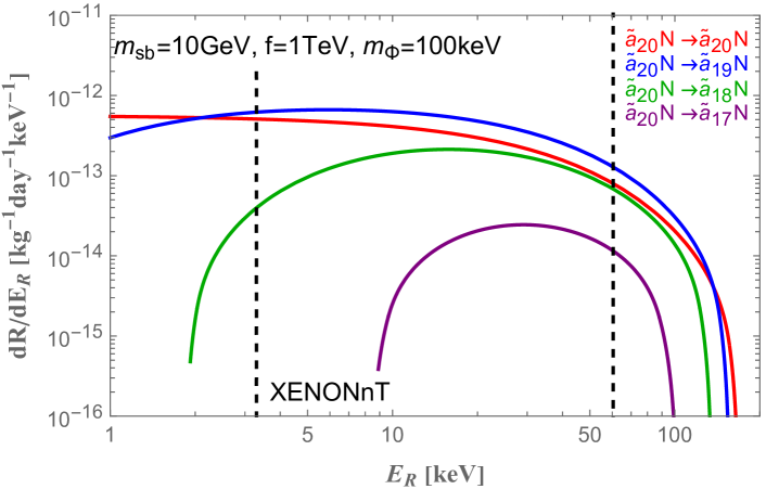
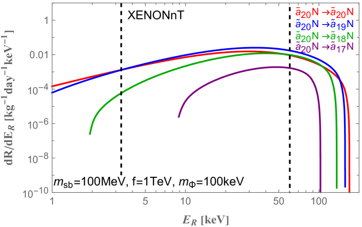
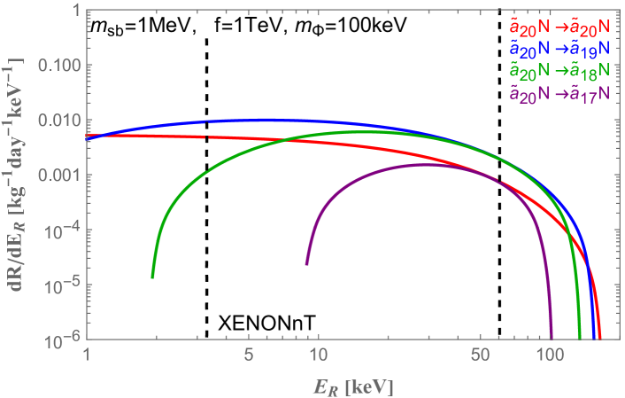
Figure 6: The differential event rate are shown for the inverted ordering case. We take $m_{\chi_{1}}=100$ GeV, $f_{a}=1$ TeV and $m_{\Phi}=100$keV. From top to bottom figures, we take $m_{sb}=10,10^{-1},10^{-3}$ GeV, respectively. Here we can see three inelastic scattering processes.

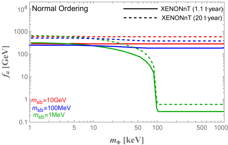
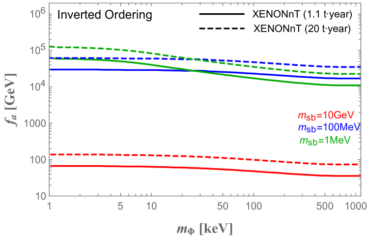
Figure 7: The XENONnT bounds are shown for the normal (uppper) and inverted (lower) mass ordering. The solid (dashed) lines represent current (future) XENONnT experimental bounds. We have taken the DM mass $100$ GeV for both cases and used $m_{\rm sb}=10(\text{Red}),~{}10^{-1}(\text{Blue}),~{}10^{-3}(\text{Green})$ GeV, respectively.

For the numerical analyses, we consider a benchmark scenario with $\xi=1$, $q=2$ and $N=20$, so we achieve a large hierarchy $q^{N}\sim 10^{6}$. In this case, the QCD axion is realized by the zero-mode axion ($a_{0}$) when $f_{a}\gtrsim 1$ TeV and we have 21 axions and 21 axinos which are involved in the scattering processes.

In Fig. 6, we show the differential event rates, $dR/dE_{R}$, of the elastic and inelastic processes in the inverted ordering case. Here we have used $f_{a}=1$ TeV and $m_{\Phi}=100$ keV. We consider three different values of $m_{sb}$ to see the results from the heavy and light axion cases. For $m_{\Phi}=100$ keV, we can see only three inelastic scattering processes. When $m_{\Phi}\leq\mathcal{O}(10)$ keV, all inelastic scattering processes are involved in the DM-nucleon scattering. In the inverted ordering case, at least one inelastic scattering channel is included in the XENONnT analyses for $m_{\Phi}{\;\raise 1.29167pt\hbox{$<$\kern-7.5pt\raise-4.73611pt\hbox{$\sim$}}\;}700$ keV. In the normal ordering case, on the other hand, at least one inelastic process is involved for $m_{\Phi}{\;\raise 1.29167pt\hbox{$<$\kern-7.5pt\raise-4.73611pt\hbox{$\sim$}}\;}100$ keV, so we can see more inelastic processes for fairly small values of $m_{\Phi}$. The difference between the normal and inverted ordering cases originates from the intrinsic structure of CW spectrum where the zero-indexed states ($a_{0}$, $s_{0}$, $\tilde{a}_{0}$) are relatively isolated from the other states. In the inverted ordering case, therefore, the lightest axino ($\tilde{a}_{20}$) can be more easily excited to the heavier modes ($\tilde{a}_{19}$, $\tilde{a}_{18}$, $\cdots$) than it is in the normal ordering case.

As we have seen in Fig. 4, the available range of recoil energy shrinks as the mass difference increases. This is also seen in Fig. 6. The full $E_{R}$ region of XENONnT is available for the elastic processes ($\tilde{a}_{20}N\to\tilde{a}_{20}N$) and two inelastic process ($\tilde{a}_{20}N\to\tilde{a}_{19}N$ and $\tilde{a}_{20}N\to\tilde{a}_{18}N$) while one inelastic process ($\tilde{a}_{20}N\to\tilde{a}_{17}N$) is not accessible for $E_{R}\lesssim 9$ keV.

In Fig. 7, we show the XENONnT bound on $(m_{\Phi},f_{a})$-plane. We take the lightest axino mass $100$ GeV and three different $m_{sb}=10$, $10^{-1}$, $10^{-3}$ GeV. The solid (dashed) lines represent the current (future) bounds from the XENONnT experiment. In order to derive the bounds, we use the same parameters as we did in Sec. II and III: recoil energy range above 10% total efficiency in range of $3.3~{}{\rm keV_{NR}}$ to $60.5~{}{\rm keV_{NR}}$ and 2.3 events expected in the 90% confidence level in the null hyperthesis. We use $1.1$ t$\cdot$year for the current bound and $20$ t$\cdot$year for the future prospects.

In the case of the normal axino mass ordering, the XENONnT bounds are of the same order for the light axions ($m_{\rm sb}=1$ MeV) and heavy axions ($m_{\rm sb}=100$ MeV and $10$ GeV). For the light axion case ($m_{\rm sb}=1$ MeV), the differential cross section is close to the approximate formula in Eq. (64), and the bound for $f_{a}$ reaches around $300$ GeV with the current data and $600$ GeV with the expected future prospect. As $m_{\Phi}$ increases, less inelastic processes are accessible and thus the total event rate decreases. For $m_{\Phi}\gtrsim 100$ keV, no inelastic processes are viable in the $E_{R}$ range of XENONnT, so the only elastic scattering can survive and the total cross section undergoes an additional $|{\cal O}_{N0}|^{2}\sim 1/q^{2N}$ suppression which is shown in the second line of Eq. (64). This suppression is transferred to the sensitivity to the $f_{a}$ bound by the factor $\sqrt{1/q^{2N}}\sim 1/1000$, so the XENONnT bound reaches only to around $300$ MeV with the current data and $600$ MeV with the expected future prospect. This small values actually do not make any sensible bounds for the model because the effective theory approach for the SUSY axion model breaks down at this scale. For the heavy axion cases ($m_{\rm sb}=100$ MeV and $10$ GeV), the total scattering process follows the approximate relation in Eq. (66). Since we consider cases with small $m_{\Phi}$, the axion masses are determined dominantly by the $m_{\rm sb}$-dependent term in Eq. (53). The eigenvalues $\lambda_{k}$ in Eq. (40) varies in range from $(q-1)^{2}$ to $(q+1)^{2}$, which are of order unity. We can take a crude simplification for the second term of Eq. (65):

$$\sum_{l=1}^{N}{\mathbf{O}}_{Nl}{\mathbf{O}}_{kl}\frac{1}{m_{a_{l}}^{2}}\simeq\frac{1}{m_{\rm sb}^{2}}\sum_{l=0}^{N}{\mathbf{O}}_{Nl}{\mathbf{O}}_{kl}\simeq\frac{\delta_{Nk}}{m_{\rm sb}^{2}}\,.$$ (67)

The total cross section becomes

$$\frac{d\sigma_{\rm tot}}{dE_{R}} \simeq \frac{F_{\tilde{G}}^{2}(E_{R})}{8\pi f_{a}^{4}v^{2}m_{N}}\frac{{\cal N}_{0}^{4}}{q^{2N}}\sum_{j,k=0}^{N}\left|\frac{\mathbf{O}_{ki}\mathbf{O}_{kj}}{q^{k}}\right|^{2}$$ (68)

$$+\frac{E_{R}^{2}m_{N}F_{\tilde{G}}^{2}(E_{R})}{2\pi f_{a}^{4}v^{2}}\frac{1}{m_{\rm sb}^{4}}\sum_{j}|\mathbf{O}_{Ni}\mathbf{O}_{Nj}|^{2}\,.$$

Here the sum of $j$ must be conducted for viable processes. For the normal mass ordering ($i=0$), the first term in Eq. (68) is dominant. Since the sum of $k$ is not much smaller than unity for $i=0$, Eq. (68) is almost the same as the light axion case described by Eq. (64). This feature clearly appears in the upper panel of Fig. 7.

In the case of the inverted axino mass ordering, the XENONnT bounds for the light axion case ($m_{\rm sb}=1$ MeV) follows Eq. (64) as in the case of the normal axino mass ordering. In this case, however, there is no suppression in $\mathbf{O}_{Ni}$ for $i=N$, so we obtain better sensitivity than that in the normal ordering case by a factor of $\sim 10^{2}$. For $m_{\rm sb}=100$ MeV, the total cross section is dominantly determined by the second term of Eq. (68), and it gives weaker sensitivity. For $m_{\rm sb}=10$ GeV, the total cross section is dominantly determined by the first term of Eq. (68). Differently from the normal mass ordering case, the sum of $k$ is highly suppressed for $i=N$. Hence the bound is much weaker than that for the light axion case by a factor of $\sim 10^{-3}$.

Before closing this section, it is worth mentioning the possible constraints on the benchmark scenarios discussed here. Since there are many axion states, sort of constraints may be applicable from the collider Mimasu:2014nea ; Bauer:2017ris , flavor probes Bauer:2021mvw , beam dump experiments Dobrich:2015jyk , and cosmology/astrophysics Depta:2020wmr ; Balazs:2022tjl . Some constraints originate from the axion-photon interaction. This is also applicable since we need to introduce the axion-photon coupling for the light axions to decay although the coupling itself does not alter our analyses given in this section. Since we need to require $f_{a}\gtrsim 1$ TeV, the collider bounds are almost irrelevant while some beam dump experiments produce marginal constraints for $m_{\rm sb}\lesssim 100$ MeV (corresponding to $m_{a_{l}}\sim{\cal O}(100)$ MeV for $l\neq 0$). Meanwhile, the flavor bounds are applicable if the axions have flavor-changing couplings with quarks and leptons which are not in our interest. The most stringent constraints, indeed, are derived from the cosmology/astrophysics. Similar to those from the beam dump experiments, there are marginal constraints for $m_{\rm sb}\lesssim 100$ MeV and $f_{a}\lesssim 1$ TeV. In this respect, the bounds for the small axion mass case ($m_{\rm sb}=1$ MeV) in Fig. 7 are not fully appreciated. The heavy axion cases ($m_{\rm sb}=100$ MeV and $10$ GeV) can, on the other hand, provide meaningful bounds for the model where the XENONnT results are sensitive to some viable parameter region for the inverted mass ordering case. The normal mass ordering case will also attain the relevant bounds for the future prospects of XENONnT.

VI Conclusions

The DM-nucleon scattering process relies on how DM particles interact with the SM particles. The massive part of DM study is based on the assumption that DM has interactions of order the weak scale. In this respect, it has been studied that the DM-nucleon scattering process is mediated by the weak gauge bosons, Higgs boson, neutrinos, or new gauge bosons with weak scale couplings. In this paper, we considers a new possibility where the DM-nucleon scattering process is mediated by the axions. If the axions couple to the gluons via the QCD anomaly coupling, i.e., $aG\tilde{G}$, the coupling induces the CP-odd gluonic current and determines the gluon form factor of the nucleon. Hence the DM-nucleon scattering process is made by exchanging the axion states as shown in Fig. 1.

The simplest model can be built with the QCD axion because it is a necessary ingredient to solve the strong CP problem. The QCD axion, however, has too small interactions with the gluons to be detected in the current experiments. Instead, we can introduce a non-QCD axion which can mediate DM-nucleon scattering process. We consider a toy model with a non-QCD axion coupled to a Majorana DM particle in Sec. II. We study how the CP-odd gluonic current contributes to the DM-nucleon scattering and show it can make relevant constraints from the current XENONnT results as shown in Fig. 2.

We extend our scope into the multi-component DM sector resulting in the axion-mediated inelastic scattering in Sec. III. The DM inelastic scattering can be realized in some $E_{R}$ range of the XENONnT experiment for the given mass difference $\delta$. The leading order calculation for the square of the matrix element does not depend on the $\delta$, so we can simply obtain the differential cross section for both the elastic and inelastic processes in Eq. (28). In Fig. 5, we show the XENONnT bounds for the 2-component model, and the bounds are similar to the single component case.

In Sec. IV, we consider the SUSY axion model to realize the QCD axion and the axion-mediated DM which contain inelastic scattering processes. In this model, the lightest axion can be a DM component and produce the DM-nucleon scattering processes mediated by the axions. From the study on the CP-odd gluonic current and kinematics for the inelastic scattering, we calculate the possible elastic and inelastic processes and show the current and future bounds for the model from the XENONnT experiments in Sec. V. The current XENONnT data already constrain some region of the parameter space for the inverted axino mass ordering case while more data are required for achieving the relevant constraints for the normal ordering case.

For conclusions, the axion-mediated process can provide substantial contributions to the DM-nucleon scattering for both the elastic and inelastic cases. The realistic scenarios can be accomplished from the SUSY CW axion model and and the XENONnT results can reach significant sensitivity for some parameter region of the model.

- (1) Planck Collaboration, N. Aghanim et al., “Planck 2018 results. VI. Cosmological parameters,” Astron. Astrophys. 641 (2020) A6, arXiv:1807.06209 [astro-ph.CO]. [Erratum: Astron.Astrophys. 652, C4 (2021)].
- (2) eBOSS Collaboration, S. Alam et al., “Completed SDSS-IV extended Baryon Oscillation Spectroscopic Survey: Cosmological implications from two decades of spectroscopic surveys at the Apache Point Observatory,” Phys. Rev. D 103 (2021) no. 8, 083533, arXiv:2007.08991 [astro-ph.CO].
- (3) DES Collaboration, T. M. C. Abbott et al., “Dark Energy Survey Year 3 results: Cosmological constraints from galaxy clustering and weak lensing,” Phys. Rev. D 105 (2022) no. 2, 023520, arXiv:2105.13549 [astro-ph.CO].
- (4) G. Bertone and D. Hooper, “History of dark matter,” Rev. Mod. Phys. 90 (2018) no. 4, 045002, arXiv:1605.04909 [astro-ph.CO].
- (5) G. Jungman, M. Kamionkowski, and K. Griest, “Supersymmetric dark matter,” Phys. Rept. 267 (1996) 195–373, arXiv:hep-ph/9506380.
- (6) G. Bertone, D. Hooper, and J. Silk, “Particle dark matter: Evidence, candidates and constraints,” Phys. Rept. 405 (2005) 279–390, arXiv:hep-ph/0404175.
- (7) H. Goldberg, “Constraint on the Photino Mass from Cosmology,” Phys. Rev. Lett. 50 (1983) 1419. [Erratum: Phys.Rev.Lett. 103, 099905 (2009)].
- (8) J. R. Ellis, J. S. Hagelin, D. V. Nanopoulos, and M. Srednicki, “Search for Supersymmetry at the anti-p p Collider,” Phys. Lett. B 127 (1983) 233–241.
- (9) K. R. Dienes, E. Dudas, and T. Gherghetta, “Grand unification at intermediate mass scales through extra dimensions,” Nucl. Phys. B 537 (1999) 47–108, arXiv:hep-ph/9806292.
- (10) H.-C. Cheng, K. T. Matchev, and M. Schmaltz, “Radiative corrections to Kaluza-Klein masses,” Phys. Rev. D 66 (2002) 036005, arXiv:hep-ph/0204342.
- (11) M. Cirelli, N. Fornengo, and A. Strumia, “Minimal dark matter,” Nucl. Phys. B 753 (2006) 178–194, arXiv:hep-ph/0512090.
- (12) B. Patt and F. Wilczek, “Higgs-field portal into hidden sectors,” arXiv:hep-ph/0605188.
- (13) B. Holdom, “Two U(1)’s and Epsilon Charge Shifts,” Phys. Lett. B 166 (1986) 196–198.
- (14) A. Falkowski, J. Juknevich, and J. Shelton, “Dark Matter Through the Neutrino Portal,” arXiv:0908.1790 [hep-ph].
- (15) G. Arcadi, M. Dutra, P. Ghosh, M. Lindner, Y. Mambrini, M. Pierre, S. Profumo, and F. S. Queiroz, “The waning of the WIMP? A review of models, searches, and constraints,” Eur. Phys. J. C 78 (2018) no. 3, 203, arXiv:1703.07364 [hep-ph].
- (16) R. D. Peccei and H. R. Quinn, “CP Conservation in the Presence of Instantons,” Phys. Rev. Lett. 38 (1977) 1440–1443. [,328(1977)].
- (17) S. Weinberg, “A New Light Boson?,” Phys. Rev. Lett. 40 (1978) 223–226.
- (18) F. Wilczek, “Problem of Strong and Invariance in the Presence of Instantons,” Phys. Rev. Lett. 40 (1978) 279–282.
- (19) J. E. Kim, “Weak Interaction Singlet and Strong CP Invariance,” Phys. Rev. Lett. 43 (1979) 103.
- (20) M. A. Shifman, A. Vainshtein, and V. I. Zakharov, “Can Confinement Ensure Natural CP Invariance of Strong Interactions?,” Nucl. Phys. B 166 (1980) 493–506.
- (21) A. Zhitnitsky, “On Possible Suppression of the Axion Hadron Interactions. (In Russian),” Sov. J. Nucl. Phys. 31 (1980) 260.
- (22) M. Dine, W. Fischler, and M. Srednicki, “A Simple Solution to the Strong CP Problem with a Harmless Axion,” Phys. Lett. B 104 (1981) 199–202.
- (23) L. Abbott and P. Sikivie, “A Cosmological Bound on the Invisible Axion,” Phys. Lett. B 120 (1983) 133–136.
- (24) J. Preskill, M. B. Wise, and F. Wilczek, “Cosmology of the Invisible Axion,” Phys. Lett. B 120 (1983) 127–132.
- (25) M. Dine and W. Fischler, “The Not So Harmless Axion,” Phys. Lett. B 120 (1983) 137–141.
- (26) M. S. Turner, “Cosmic and Local Mass Density of Invisible Axions,” Phys. Rev. D 33 (1986) 889–896.
- (27) P. Sikivie, “Experimental Tests of the Invisible Axion,” Phys. Rev. Lett. 51 (1983) 1415–1417. [Erratum: Phys.Rev.Lett. 52, 695 (1984)].
- (28) A. Arvanitaki, S. Dimopoulos, S. Dubovsky, N. Kaloper, and J. March-Russell, “String Axiverse,” Phys. Rev. D 81 (2010) 123530, arXiv:0905.4720 [hep-th].
- (29) K. Mimasu and V. Sanz, “ALPs at Colliders,” JHEP 06 (2015) 173, arXiv:1409.4792 [hep-ph].
- (30) M. Bauer, M. Neubert, and A. Thamm, “Collider Probes of Axion-Like Particles,” JHEP 12 (2017) 044, arXiv:1708.00443 [hep-ph].
- (31) M. Bauer, M. Neubert, S. Renner, M. Schnubel, and A. Thamm, “Flavor probes of axion-like particles,” JHEP 09 (2022) 056, arXiv:2110.10698 [hep-ph].
- (32) B. Döbrich, J. Jaeckel, F. Kahlhoefer, A. Ringwald, and K. Schmidt-Hoberg, “ALPtraum: ALP production in proton beam dump experiments,” JHEP 02 (2016) 018, arXiv:1512.03069 [hep-ph].
- (33) P. F. Depta, M. Hufnagel, and K. Schmidt-Hoberg, “Robust cosmological constraints on axion-like particles,” JCAP 05 (2020) 009, arXiv:2002.08370 [hep-ph].
- (34) C. Balázs et al., “Cosmological constraints on decaying axion-like particles: a global analysis,” JCAP 12 (2022) 027, arXiv:2205.13549 [astro-ph.CO].
- (35) K. Choi, H. Kim, and S. Yun, “Natural inflation with multiple sub-Planckian axions,” Phys. Rev. D 90 (2014) 023545, arXiv:1404.6209 [hep-th].
- (36) K. Choi and S. H. Im, “Realizing the relaxion from multiple axions and its UV completion with high scale supersymmetry,” JHEP 01 (2016) 149, arXiv:1511.00132 [hep-ph].
- (37) D. E. Kaplan and R. Rattazzi, “Large field excursions and approximate discrete symmetries from a clockwork axion,” Phys. Rev. D 93 (2016) no. 8, 085007, arXiv:1511.01827 [hep-ph].
- (38) T. Higaki, K. S. Jeong, N. Kitajima, and F. Takahashi, “The QCD Axion from Aligned Axions and Diphoton Excess,” Phys. Lett. B 755 (2016) 13–16, arXiv:1512.05295 [hep-ph].
- (39) K. J. Bae and S. H. Im, “Supersymmetric Clockwork Axion Model and Axino Dark Matter,” Phys. Rev. D 102 (2020) no. 1, 015011, arXiv:2004.05354 [hep-ph].
- (40) D. Tucker-Smith and N. Weiner, “Inelastic dark matter,” Phys. Rev. D 64 (2001) 043502, arXiv:hep-ph/0101138.
- (41) K. Choi, S. H. Im, H. J. Kim, and H. Seong, “Precision axion physics with running axion couplings,” JHEP 08 (2021) 058, arXiv:2106.05816 [hep-ph].
- (42) F. Bishara, J. Brod, B. Grinstein, and J. Zupan, “DirectDM: a tool for dark matter direct detection,” arXiv:1708.02678 [hep-ph].
- (43) Flavour Lattice Averaging Group Collaboration, S. Aoki et al., “FLAG Review 2019: Flavour Lattice Averaging Group (FLAG),” Eur. Phys. J. C 80 (2020) no. 2, 113, arXiv:1902.08191 [hep-lat].
- (44) J. Fan, M. Reece, and L.-T. Wang, “Non-relativistic effective theory of dark matter direct detection,” JCAP 11 (2010) 042, arXiv:1008.1591 [hep-ph].
- (45) M. Cirelli, E. Del Nobile, and P. Panci, “Tools for model-independent bounds in direct dark matter searches,” JCAP 10 (2013) 019, arXiv:1307.5955 [hep-ph].
- (46) J. Bland-Hawthorn and O. Gerhard, “The Galaxy in Context: Structural, Kinematic, and Integrated Properties,” Ann.Rev.Astron.Astrophys. 529 (2016) no. 54, 529–596, arXiv:1602.07702 [astro-ph.GA].
- (47) R. Abuter et al., “Improved GRAVITY astrometric accuracy from modeling optical aberrations,” Astron.Astrophys. 647 (2021) 17.
- (48) J. Bramante, P. J. Fox, G. D. Kribs, and A. Martin, “Inelastic frontier: Discovering dark matter at high recoil energy,” Phys. Rev. D 94 (2016) no. 11, 115026, arXiv:1608.02662 [hep-ph].
- (49) XENON Collaboration, E. Aprile et al., “First Dark Matter Search with Nuclear Recoils from the XENONnT Experiment,” Phys. Rev. Lett. 131 (2023) no. 4, 041003, arXiv:2303.14729 [hep-ex].
- (50) G. F. Giudice and M. McCullough, “A Clockwork Theory,” JHEP 02 (2017) 036, arXiv:1610.07962 [hep-ph].