Mapping Solutions in Nonmetricity Gravity: Investigating Cosmological Dynamics in Conformal Equivalent Theories
Abstract
We investigate the impact of conformal transformations on the physical properties of solution trajectories in nonmetricity gravity. Specifically, we explore the phase space and reconstruct the cosmological history of a spatially flat Friedmann–Lemaître–Robertson–Walker universe within scalar-nonmetricity theory in both the Jordan and Einstein frames. A detailed analysis is conducted for three connections defined in the coincident and non-coincident gauges. Our findings reveal the existence of a unique one-to-one correspondence for equilibrium points in the two frames. Furthermore, we demonstrate that solutions describing accelerated universes remain invariant under the transformation that relates these conformally equivalent theories.
I Introduction
Conformal transformations are mappings that reshape geometric objects into other forms, wherein the distances between points are not conserved. However, these transformations maintain the angles at each point on the object. A subset of conformal transformations is known as isometries, wherein the distances between points remain unchanged. Isometries and conformal transformations have various applications in different branches of physical science, offering a systematic approach to analyze the physical world conf .
In Newtonian physics, isometries are instrumental in understanding the conservation laws governing momentum and angular momentum as they pertain to Euclidean geometry con1 . Similarly, in gravitational physics, the conservation laws associated with time-like geodesics are related to the presence of isometries for the background geometry. On the other hand, conformal transformations are used to construct conservation laws for the null-geodesics con2 .
Conformal transformations are crucial in gravitational physics and cosmology framework, particularly in scalar-tensor theories ref1 ; ref2 . These transformations can transit between the Jordan and Einstein frames and vice versa. In scalar-tensor theories, a scalar field is nonminimally coupled to gravity, introducing a coupling function in the gravitational Lagrangian to describe the interaction with the scalar field ref3 . Through the application of a conformal transformation, the coupling function can be eliminated from the gravitational Lagrangian. This results in an equivalent theory where the gravitational dynamics involve a minimally coupled scalar field defined in the Einstein frame. It is important to note that introducing the coupling function to the metric tensor through the conformal transformation leads to differences in the physical quantities derived from the same solution trajectories ref4 .
This mathematical approach enables the construction of new solutions for conformally equivalent theories. Additionally, researchers have demonstrated that applying conformal transformations can be instrumental in avoiding cosmological singularities kam1 . Indeed, singular solutions in the one frame can correspond to nonsingular solutions for the other frame and vice versa ll1 ; ll2 ; ll3 . Thus, conformal transformations are a powerful tool for understanding the dynamics of scalar-tensor theories in gravitational physics and cosmology. Numerous studies have extensively investigated physical quantities within the context of exact solutions in both the Einstein and Jordan frames jd1 ; jd2 ; jd3 ; jd4 ; jd5 ; jd6 . Despite this wealth of research, the question of which frame is preferred remains unanswered fr1 .
In this study, we deal with the effects of conformal transformations on the physical properties of conformal equivalent theories in scalar-tensor theories in the framework of symmetric teleparallel gravity. This theory, which from now we will call it scalar-nonmetricity, which is an extension of Symmetric Teleparallel General Relativity (STGR) Nester:1998mp where a scalar field lies on the physical space with a nonzero interaction function with the fundamental Lagrangian of the theory is the nonmetricity scalar sc1 . Scalar-nonmetricity theory is the analogue of the scalar-curvature sf1 and scalar-torsion theories sf4 for the third invariant of the trinity of gravity trinity . STGR and its extensions Koivisto2 ; Koivisto3 ; rev10 have been introduced as theoretical frameworks aimed at addressing fundamental cosmological phenomena, specifically the cosmic acceleration and the formation of the universe ft1 ; ft2 ; ft3 ; ft5 ; ft6 ; fq2 ; fq3 ; fq4 ; fq6 ; fq8 ; fq9 ; fq10 ; fq11 ; fq12 ; fq14 ; fq15 .
In a recent work, bdpal , a Brans-Dicke analogue was introduced within the framework of symmetric teleparallel theory. This model, akin to the original Brans-Dicke theory, introduced by Brans , incorporates a free parameter analogous to the Brans-Dicke parameter denoted as omegaBDGR . Notably, when this parameter is set to zero, the model describes the -theory. This construction parallels the way in which the Brans-Dicke theory allocates degrees of freedom for the -theory of gravity s01 . For the Brans-Dicke analogue in STGR, new cosmological solutions are determined bdpal , and the impact of the conformal transformation of the physical variables are examined. It was found that the generic properties of exact solutions remain invariant under the conformal transformation bdpal .
To conduct a detailed analysis of the impact of conformal transformations on the physical properties of solution trajectories in scalar-nonmetricity theory, we focus on investigating the phase space for these trajectories within the context of a spatially flat Friedmann-Lemaître-Robertson-Walker (FLRW) universe. Our specific goal is to reconstruct the cosmological history as conformally equivalent theories describe, allowing us to compare the cosmic evolution and relevant cosmological epochs. The structure of the paper is as follows.
In Section II, we provide the fundamental properties and definitions of scalar-nonmetricity gravity. This theory is a generalization of scalar-curvature theories within the symmetric teleparallel formalism, where the scalar field is nonminimally coupled to the nonmetricity scalar . Additionally, we go deeper into the effects of conformal transformations and determine the conformal equivalent theory. Our focus centers on the Brans-Dicke analogue within nonmetricity gravity. In Section III, we specifically concentrate on this Brans-Dicke analogue. Here, we present the field equations applicable to a spatially flat Friedmann–Lemaître–Robertson–Walker (FLRW) geometry for three distinct sets of the connection. Demonstrating that these field equations permit a minisuperspace description, we proceed to formulate the corresponding point-like Lagrangians for the nonmetricity Brans-Dicke model in both the Jordan and (pseudo-) Einstein frames. As we shall see in the following, although the conformal equivalent theory of the scalar field is not coupled to the nonmetricity Lagrangian, there exists a nontrivial coupling function with another geometric invariant related to the Lagrangian of the nonmetricity theory. Hence, we shall call that the theory is defined in the a (pseudo-) Einstein frame.
The phase-space analysis of the field equations and the reconstruction of the cosmological history are presented in the respective Sections IV, V and VI for the three different connections. Specifically, we employ dimensionless variables within the -normalization approach to determine equilibrium points for the field equations. Our analysis extends to investigating the physical properties of asymptotic solutions at these equilibrium points and their stability properties. The insights gained from this analysis are then utilized to define constraints for the theory’s viability. Furthermore, a similar analysis is conducted for the conformal equivalent theory defined in the Einstein frame to explore the impact of conformal transformations on the physical properties of solution trajectories. This comparative analysis reveals a one-to-one correspondence between equilibrium points and their associated physical properties in both theories. Finally, we present our conclusions in Section VII.
II Scalar-nonmetricity theory
We consider the scalar-nonmetricity theory of gravity described by the Action Integral sc1
| (1) |
where is a scalar field with potential function , is the metric tensor of a four-dimensional manifold with the symmetric connection which inherits the symmetries of the metric tensor and defined the covariant derivative operator .
The gravitational scalar which is is the nonmetricity scalar, is defined as rev10
| (2) |
where is the nonmetricity tensor, that is,
| (3) |
Furthermore, function in (1) is the coupling function between the scalar field and the nonmetricity scalar; similarly to the coupling function of the scalar field with the Ricci scalar in the scalar-curvature theory. On the other hand, function can be eliminated with the introduction of the new scalar field ; where Action (1) reads sc1
| (6) |
Variation with respect to the metric tensor in (1) leads to the field equations sc1 ; sc2
| (7) |
while variation with respect to the connection leads to the equations
| (8) |
Finally, variation with respect to the scalar field in (1) provides the modified Klein-Gordon equation
| (9) |
It is important to observe that for , , the latter field equations take the functional form of -theory sc1 , where now and , which means that the Action (1) is equivalent to that of -theory Koivisto2 ; Koivisto3 .
II.1 Conformal equivalent theory
Let be two metric tensors that share the same conformal algebra, meaning that the metrics are conformally related in such a way that
where is the so-called conformal function.
The nonmetricity tensors , for the two conformal related metrics are related as gg1
| (10) |
and the corresponding nonmetricity scalars and are related
| (11) |
Assume the Action Integral (1) for the metric tensor , that is,
| (12) |
Then, the conformal equivalent theory is
| (13) |
where is the boundary term relates the nonmetricity scalar and the Ricci scalar for the Levi-Civita connection of the metric tensor sc1 .
We introduce the new scalar field
| (14) |
and the latter Action Integral becomes
| (15) |
II.2 Nonmetricity Brans-Dicke theory
We consider the scalar-nonmetricity theory with and in which This theory can be seen as the extension of the Brans-Dicke theory in nonmetricity scalar, where plays the role of the Brans-Dicke parameter. Indeed, the Action Integral (1) reads gg1 ; bdpal
| (16) |
An equivalent way to write the latter theory is by introducing the dilaton field , such that the latter Action Integral is
| (17) |
Moreover, the action integral for the conformally equivalent theory is given by
| (18) |
III FLRW Cosmology
In this study, we investigate the effects of conformal transformation in the cosmological evolution and cosmological history. Specifically, we consider a universe described by the isotropic and homogeneous FLRW geometry, with element
| (19) |
in which is the lapse function, is the scale factor denotes the radius of the universe. The Hubble function is defined as, , where . denotes the spatial curvature, for , the universe is spatially flat, corresponds to a closed FLRW geometry and describes an open universe.
For this cosmological model, we study the dynamics of the field equations in scalar-nonmetricity theory for the dilaton field (17) and will reconstruct the cosmological history. Furthermore, we will perform the same analysis for the conformal equivalent theory (18). We shall compare the two cosmological histories and the provided cosmological eras by the two different cosmological models. From this analysis, we can infer the effects of the conformal transformation on the physical solutions in nonmetricity theories.
In General Relativity, the definition of the connection is unique; it is the Levi-Civita, in nonmetricity theory, the connection is not necessarily unambiguously defined. For the FLRW geometry, four different families of connections are used to describe diagonal field equations Hohmann . For the spatially flat universe, there are three different families of connections; on the other hand, for , the connection is uniquely defined. In the following, we consider that the spatial curvature is zero.
For , the common nonzero components of the of the three different connections , and are Hohmann
while the additional nonzero components for each connection , and are Hohmann
and
where a dot means derivative with respect to the time parameter , i.e. .
Consequently, the nonmetricity scalars and the corresponding boundary terms for the first connection read anbb
| (20) |
| (21) |
for the second connection are calculated anbb
| (22) |
| (23) |
while for the third connection we calculate the scalars anbb
| (24) |
| (25) |
III.1 Minisuperspace description for the dilaton field
For each connection the resulting field equations are different. That is, because the coupling between the scalar field with the nonmetricity scalar leads to the introduction of dynamical degrees of freedom related to the function which defines the connection. Connection is defined in the so-called coincident gauge where the equation of motion (8) is trivially satisfied. However, that is not true for the other three families of connections that are defined in the noncoincident gauge.
To understand the effects of the connection in the field equations, we follow the procedure described in mini and we write the corresponding point-like Lagrangian for the field equations for each connection.
For the first connection, namely , the corresponding point-like Lagrangian is
| (26) |
Similarly, for the second connection, , the field equations follow from the variation of the point-like Lagrangian function anbb
| (27) |
in which .
Finally, for connection and the Lagrangian function is
| (28) |
III.1.1 Conformal transformation
We can also write the minisuperspace Lagrangians and the conformal equivalent theories. Indeed, the FLRW line element
| (29) |
with , is conformally related to the line element (19) with conformal factor the coupling function .
By applying the latter transformation in the action
| (30) |
for each of the Lagrangian functions (26), (27) and (28); we end with the following conformal equivalent point-like Lagrangians
| (31) |
| (32) |
and
| (33) |
where now
We remark that the conformal transformation eliminates the coupling function in the Lagrangian, however, introduces the dynamical components in all the set of field equations. Moreover, for the scalar field potential we consider the exponential function, that is, .
IV Phase-space analysis for connection
For the connection defined in the coincident gauge and for , and from the point-like Lagrangian (26) we determine the cosmological field equations,
| (34) | ||||
| (35) | ||||
| (36) |
where is the Hubble function.
The latter equations can be written in the equivalent form
| (37) |
in which , are the effective fluid energy density and pressure component for the geometric fluid, defined
| (38) | ||||
| (39) |
To examine the cosmological dynamics and reconstruct the cosmological history for this gravitational model we introduce dimensionless variables in the -normalization consideration.
We define the new dependent variables
| (40) |
and the independent variable
Hence, the field equations with the use of the dimensionless variables are expressed as follow
| (41) | ||||
| (42) |
with constraint equation
| (43) |
Furthermore, the equation of state parameter is expressed as
| (44) |
With the application of the constraint equation (43) we can reduce the dimension of the dynamical system (41), (42) by one. Thus we end with the equation
| (45) |
The equilibrium points of the latter equation are
Point exist for , and describe a universe dominated by a fluid source with the equation of state parameter . The latter asymptotic solution describes a de Sitter universe for . On the other hand, points are real for . The equation of state parameters for the asymptotic solutions at these two points are . Thus and . Hence, point describes an accelerated universe for .
In order to investigate the stability properties of the linearized system we calculate the eigenvalues of the linearized equation (45). They are , . Thus, point is an attractor for or . Furthermore, point is attractor for and and is attractor for and .
IV.1 Conformal equivalent theory
Consider now the field equations for the conformal equivalent theory described by the Lagrangian function (31), the equations are
| (46) | ||||
| (47) | ||||
| (48) |
where we have assumed .
Equivalently they can be expressed
| (49) |
with effective fluid components
| (50) | ||||
| (51) |
in which is the Hubble function for the conformal equivalent theory.
We follow the same procedure as before and we introduce the dimensionless variables
Hence, the field equations in the set of variables read
| (52) | ||||
| (53) |
and algebraic constraint
| (54) |
Furthermore, the equation of state parameter is defined as
| (55) |
With the application of the constraint (54) we end with the single first-order ordinary differential equation
| (56) |
The stationary points of the latter equation are
or
The equilibrium point exist always and describes a scaling solution with , while the asymptotic solution is that of the de Sitter universe when and . Furthermore, points are real for and the points describe stiff fluid solutions in which .
The eigenvalues of the linearized equation (56) near the stationary points are , . Therefore, point is an attractor for and . Similarly, point is an attractor for , , , while point is an attractor for , and . The region plots where the equilibrium points in the Einstein frame, attractors are presented in Fig. 1.

| Point | Existence | Acceleration? | Attractor? | |
| Equilibrium points for Connection in the Jordan frame | ||||
| Always | Yes | , | ||
| No | , | |||
| Yes | , | |||
| Equilibrium points for Connection in the Einstein frame | ||||
| Always | Yes | Fig. 1 | ||
| No | Fig. 1 | |||
The results of this Section are summarized in Table 1. We observe that for this cosmological model, there exists a one-to-one connection between the stationary points in the two frames. For , only points and exist. Indeed, every asymptotic solution described by the point reduce to a solution described by the conformal equivalent theory by point . In general, singular solutions, are transformed into singular solutions. Except in the case for , where the singular solution at the Jordan frame reads as a de Sitter solution at the Einstein frame. Moreover, for , the asymptotic solution describes a de Sitter universe in the two frames. Furthermore, for , the additional points and exist. In the Einstein frame at these points, the asymptotic solutions describe only stiff fluid components, while in the Jordan frame, other fluid components can be described.
V Phase-space analysis for connection
We proceed our analysis with the field equations which correspond to the selection for the connection . Indeed, from the point-like Lagrangian (27) we determine the field equations anbb
| (57) | ||||
| (58) | ||||
| (59) | ||||
| (60) |
where the effective fluid components are
| (61) | ||||
| (62) |
and .
We work in the dimensionless variables
where the field equations (57)-(60) are expressed as
| (63) | ||||
| (64) | ||||
| (65) |
and constraint equation
| (66) |
Finally, the equation of state parameter is expressed as
| (67) |
By applying the constraint equation (66) the dimension of the dynamical system is reduced by one, and the stationary points are defined in the plane .
They are
where in is an arbitrary constant. Specifically describes a family of points with the equation of state parameter . Moreover, point describes the de Sitter universe with .
The eigenvalues of the two-dimensional linearized system around the stationary points are and . As a result, point is always an attractor, while for the family of points because one of the eigenvalues has zero real part, the Center Manifold Theorem (CMT) should be applied. From the latter, we will be able to show if there exists any stable submanifold when .
In order to calculate the CMT, we perform the change of variable , such that the dynamical system reduced to the following form
| (68) | ||||
| (69) |
where in the new variables points have coordinates . In order to determine the stable manifold, we assume that , where we end with the equation
| (70) |
with solutions , and .
In order to describe a stable submanifold it should hold, and . Consequently, the unique stable submanifold is the surface of points with . That means, that if the initial conditions belong to the family of points , for , the trajectory solutions will stay on the surface defined by points .
Nevertheless, variables are not constrained which means that they can take values at infinity. Thus, we should determine the existence of stationary points at the infinity regime. In order to perform such analysis we introduce the Poincare variables
and we write the two-dimensional dynamical system in the form
Infinity is reached when , thus, the admitted equilibrium points at the infinity are
We derive that the stationary points describe de Sitter universes, that is, , while points and correspond to Big Rip singularities, that is, and . As far as stability is concerned, it follows that all the stationary points at the infinity describe unstable solutions.
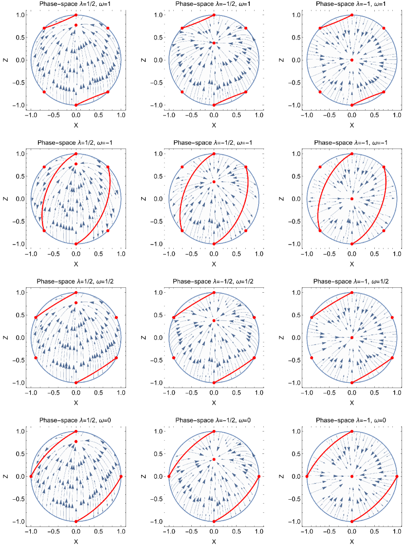
In Fig. 2 we present phase-space portraits for this dynamical system for different values of the free parameters and . We observe that in order the cosmological evolution not to suffer from a Big Rip singularity in the future, we should start from the initial conditions inside the region bounded by the family of points .
V.1 Conformal equivalent theory
We proceed with the analysis of the dynamics for the conformal equivalent theory described by the Lagrangian function (32).
For this cosmological model, the cosmological field equations are anbb
| (71) | ||||
| (72) | ||||
| (73) | ||||
| (74) |
with effective fluid components
| (75) | ||||
| (76) |
and .
We work in the dimensionless variables
where now the field equations are expressed as
| (77) | ||||
| (78) | ||||
| (79) |
and
| (80) |
with equation of state parameter
The stationary points of the latter system are defined in the two-dimensional manifold ; they are
| (81) |
Points describe a family of points which exist for . The asymptotic solutions at the points correspond to universes dominated by a stiff fluid, i.e. . Moreover, Point describes a de Sitter solution, which is a future attractor for the dynamical system; since the eigenvalues of the linearized system are . As far as the stability properties of points are concerned, we determine the two eigenvalues . Because is zero, we apply the CMT as before and we found that the stationary points do not describe stable solutions, except if the initial conditions are that defined on the family of points .
We remark that at the finite regime, there exists a one-to-one correspondence between the equilibrium points, and their asymptotic solutions, for the two conformal equivalent theories defined in the Jordan and the Einstein frames. We proceed with the analysis of the asymptotics at the infinite regime.
We define the Poincare variables
Hence, the dynamical system can be written in the following form
At infinity, the stationary points are
Similar to the conformal equivalent theory defined in the in Jordan frame, points describe de Sitter solutions, while points and correspond to Big Rip singularities, i.e. and . We omit the presentation of the stability analysis, but we conclude that all the stationary points at the infinity describe unstable solutions.
Thus, the unique attractor for this model is the de Sitter universe described by point . Additionally, we remark that there exists an one-to-one corresponds to the equilibrium points between the Jordan and the Einstein frames. The only physical solution which does not remain invariant is that described by points . Indeed the conformal equivalent points describe only stiff fluid solutions, while the solutions at the family of point can describe accelerated universes.
The results of this Section are summarized in Table 2, where the physical properties of the stationary points can be compared between the two frames.
| Point | Existence | Acceleration? | Attractor? | |
|---|---|---|---|---|
| Equilibrium points for Connection in the Jordan frame | ||||
| Yes | No | |||
| Always | Always | Always | ||
| Always | Always | No | ||
| Always | Big Rip | Always | No | |
| Always | Big Rip | Always | No | |
| Equilibrium points for Connection in the Einstein frame | ||||
| No | No | |||
| Always | Always | Always | ||
| Always | Always | No | ||
| Always | Big Rip | Always | No | |
| Always | Big Rip | Always | No | |
VI Phase-space analysis for connection
Finally, for the third connection and Lagrangian function (28) we derive the field equations
| (82) | ||||
| (83) | ||||
| (84) | ||||
| (85) |
and the fluid components are expressed as follows
| (86) | ||||
| (87) |
with .
In the dimensionless variables we work in the dimensionless variables
the field equations become
| (88) | ||||
| (89) | ||||
| (90) |
and
| (91) |
Thus, the equation of state parameter reads
| (92) |
With the use of the algebraic equation (91) the dynamical system is reduced to a two-dimensional system, where the stationary points in the finite regime are
Point exist always, however, for the rest of the points the existence conditions are, for point , ; for points , and ; point exists for . Finally, points are real when . The equation of state parameter for the effective fluid at the asymptotic solutions at the equilibrium points are , , and .
Point describes a scaling solution, where acceleration is occurred for , and for the de Sitter universe is recovered. Furthermore, corresponds to the de Sitter point, similar to point . Points describe scaling solutions, accelerated is occurred for . Last but not least, points and have the same physical properties with points and respectively.
As far as the stability properties of the stationary points are concerned, in Fig. 3 we present the regions in the space of the free variables in which points and are attractors. For point, , the eigenvalues of the linearized system have always negative real parts which means that the de Sitter solution is a future attractor. Furthermore, for point we calculate the eigenvalues and , from where it follows that the equilibrium point is an attractor when , , . Finally, for points the eigenvalues are , , from where we conclude that the solution at is always unstable and is an attractor when and .

We continue with the analysis of the dynamics at the infinity. We make use of the Poincaré variables
and the time derivative
to obtain the dynamical system is written in the form
The stationary points of the latter dynamical system at infinity are
Stationary points describe de Sitter solutions and , correspond to Big Rip singularities. It is straightforward to show that the equilibrium points at infinity do not describe any stable solution.
VI.1 Conformal equivalent theory
We proceed with the investigation of the equilibrium points for the conformal equivalent theory. Indeed, from Lagrangian (33) we derive the field equations
| (93) | ||||
| (94) | ||||
| (95) | ||||
| (96) |
for .
From the latter set of field equations, we define the components
| (97) | ||||
| (98) |
In terms of the dimensionless variables
we write the following dynamical system
| (99) | ||||
| (100) | ||||
| (101) | ||||
| (102) | ||||
| (103) |
and constraint
| (104) |
Moreover, we calculate the effective equation of state parameter
The stationary points of the latter dynamical system have the following coordinates
Point describes the de Sitter solution, , while the rest of the equilibrium points describe asymptotic solutions described by an ideal gas with effective equation of state for the points and , describe ideal gas solutions with , and . Hence, only can describe an accelerated universe when , , , and .
Furthermore, we find that the de Sitter solution described by point is always an attractor, while points is an attractor when or . For the rest of the points, the regions in the space of the free parameters where the points are attractors are presented in Fig. 4.
For the study at the infinity, we employ the Poincaré variables
and the new time variable
Thus, the dynamical system reads
The stationary points at the infinity regime are
and
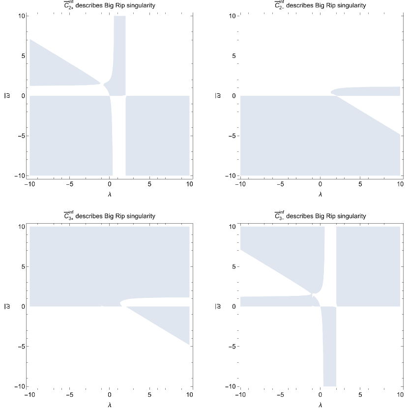
Points describe de Sitter solutions, while the new points correspond to Big Rip singularities when Moreover, points and can describe Big Rip singularities for specific values of the free parameters. In Fig. 5 we present the regions where the asymptotic solutions at these equilibrium points describe Big Rip singularities.
Finally, we find that points , and describe unstable solutions, while points are attractors for , or .
The results of this Section are summarized in Table 3.
We remark that while in the finite regime, there exists a one-to-one connection between the stationary points for the two frames, at the infinity regime there exist a new family of solutions, described by the points .
| Point | Existence | Acceleration? | Attractor? | |
| Equilibrium points for Connection in the Jordan frame | ||||
| Fig. 3 | ||||
| Always | Always | Always | ||
| , | Fig. 3 | |||
| Yes | Yes | |||
| Yes for | Yes for | |||
| Always | Always | No | ||
| Always | Big Rip | Always | No | |
| Always | Big Rip | Always | No | |
| Equilibrium points for Connection in the Einstein frame | ||||
| No | Fig. 4 | |||
| Always | Always | Always | ||
| , | No | Fig. 4 | ||
| Yes | Yes | |||
| , | No | No | ||
| Always | Yes | No | ||
| and | Fig. 5 | No | ||
| and | Fig. 5 | No | ||
| Always | Yes | |||
VII Conclusions
In this study, we investigate the effects of conformal transformations on the physical properties of solution trajectories in a scalar-nonmetricity cosmology. Specifically, within the framework of nonmetricity gravity, we consider a scalar field nonminimally coupled to the Lagrangian of STGR. Our focus is on the asymptotic dynamics of the field equations, particularly in the scenario of an isotropic and homogeneous universe described by a spatially flat FLRW line element.
In General Relativity the Ricci scalar is associated with the Levi-Civita connection for the metric tensor, while in STGR, the nonmetricity scalar depends on a connection that is not uniquely defined. We imposed conditions on the connection to fulfil the symmetries of the background spacetime, be symmetric and flat, and align with the cosmological principle for a cosmological fluid. This leads to three families of connections, each associated with a distinct nonmetricity scalar differing by a boundary term. Although these connections yield the same limit of field equations in STGR, the presence of a nonminimally coupled scalar field introduces new geometrodynamical degrees of freedom related to the boundary term. Consequently, in scalar-nonmetricity theory, the field equations exhibited dependence on the choice of connection.
For each of the three cosmological models defined by the different connections, we analyzed the phase space by identifying equilibrium points and studying their stability properties. Each equilibrium point corresponds to an asymptotic solution for cosmological evolution, allowing us to construct the cosmological history and establish constraints on the free parameters of the theory. Additionally, we applied the same analysis to the field equations of three conformal equivalent theories defined in the Einstein frame.
Comparing the physical properties of solutions at equilibrium points for the three sets of symmetries, we conclude that, regardless of the connection, there exists a one-to-one relation between equilibrium points in the Jordan and Einstein frames. Interestingly, the de Sitter universe and solutions describing Big Rip singularities remained invariant under conformal transformations. This behavior in nonmetricity gravity contrasts with that in scalar-curvature theory c0 , where singular solutions in one frame can be related to nonsingular solutions in a conformal equivalent theory and vice versa.
The debate over which frame is the “physical” one was ongoing, see the discussions c1 ; c2 ; c3 ; c4 ; c5 ; c6 ; c7 ; c8 , our study suggests that there are no significant differences in the cosmological evolution within the context of nonmetricity gravity. In future research, we plan to extend this investigation to the case of compact objects.
Acknowledgements.
KD was funded by the National Research Foundation of South Africa, Grant number 131604. AG was financially supported by FONDECYT 1200293. GL was funded by Vicerrectoria de Investigacion y Desarrollo Tecnologico (VRIDT) at Universidad Catolica del Norte through Resolución VRIDT No. 026/2023 and Resolución VRIDT No. 027/2023 and the support of Nucleo de Investigacion Geometria Diferencial y Aplicaciones, Resolución VRIDT No. 096/2022. He also acknowledges the financial support of Proyecto de Investigacion Fondecyt Regular 2023, Resolución VRIDT No. 076/2023. AP thanks the support of VRIDT through Resolución VRIDT No. 096/2022, Resolución VRIDT No. 098/2022.References
- (1) D. Beliaev, Conformal Maps and Geometry, World Scientific, New Jersey (2018)
- (2) M. Tsamparlis and A. Paliathanasis, Gen. Rel. Grav. 43, 1861 (2011)
- (3) T. Christodoulakis, N. Dimakis and P.A. Terzis, J. Phys. A: Math. Theor. 47, 095202 (2014)
- (4) V. Faraoni, Cosmology in Scalar-Tensor Gravity, Fundamental Theories of Physics vol. 139, (Kluwer Academic Press: Netherlands, 2004)
- (5) D. Keiser, Phys. Rev. D. 81, 084044 (2010)
- (6) M. Tsamparlis, A. Paliathanasis, S. Basilakos and S. Capozziello, Gen. Rel. Grav. 45, 2003 (2013)
- (7) G. Allemandi, M. Capone, S. Capozziello, M. Francaviglia, Gen. Rel. Grav. 38, 33 (2006)
- (8) A.Yu. Kamenshchik, E.O. Pozdeeva, S. Yu. Vernov, A. Tronconi and G. Venturi, Phys. Rev. D 94, 063510 (2016)
- (9) V. Faraoni and E. Gunzig, Int. J. Theor. Phys. 38, 217 (1999)
- (10) M. Postma and M. Volponi, Equivalence of the Einstein and Jordan frames, Phys. Rev. D 90, 103516 (2014)
- (11) G. Allemandi, M. Capone, S. Capozziello, M. Francaviglia, Gen. Rel. Grav. 38, 33 (2006)
- (12) Y. Fujii, Prog. Theor. Phys. 118, 983 (2007)
- (13) R.M. Avakyan, E.V. Chubaryan, G.H. Harutyunyan, A.V. Hovsepyan and A.S. Kotanjyan, J. Phys: Conf. Ser. 496, 012020 (2014)
- (14) N. Dimakis, A. Giacomini and A. Paliathanasis, Eur. Phys. J. C 78, 751 (2018)
- (15) G. Gionti S.J., Phys. Rev. D 103, 024022 (2021)
- (16) M. Galaverni, G. Gionti S.J., Universe 8, 14 (2021)
- (17) G. Gionti S.J., M. Galaverni, On the canonical equivalence between Jordan and Einstein frames, (2023) [arXiv:2310.09539]
- (18) V. Faraoni, Int. J. Theor. Phys. 38, 217 (1999)
- (19) J.M. Nester and H.-J. Yo, Chin. J. Phys. 37, 113 (1999)
- (20) L. Järv, M. Rünkla, M. Saal and O. Vilson, Phys. Rev. D 97, 124025 (2018)
- (21) V. Faraoni, Cosmology in Scalar-Tensor Gravity, Fundamental Theories of Physics vol. 139, (Kluwer Academic Press: Netherlands, 2004)
- (22) M.A. Skugoreva, E.N. Saridakis and A.V. Phys. Rev. D 91, 044023 (2015)
- (23) J. Beltran, J.L. Heisenberg and T.S. Coivisto, Universe 5, 173 (2019)
- (24) J. B. Jiménez, L. Heisenberg and T. S. Koivisto, Phys. Rev. D 98, 044048 (2018)
- (25) J. B. Jiménez, L. Heisenberg, T. S. Koivisto and S. Pekar, Phys. Rev. D 101, 103507 (2020)
- (26) L. Heisenberg, Review on f(Q) Gravity, (2023) [arXiv:2309.15958]
- (27) A. Paliathanasis, The Brans-Dicke field in Non-metricity gravity: Cosmological solutions and Conformal transformations, (2023) [arXiv:2310.16357]
- (28) C. Brans and R.H. Dicke, Phys. Rev. 124, 195 (1961)
- (29) V. Faraoni, Phys. Rev. D 59, 084021, (1999)
- (30) T.P. Sotiriou, Gravity and Scalar fields, Proceedings of the 7th Aegean Summer School: Beyond Einstein’s theory of gravity, Modifications of Einstein’s Theory of Gravity at Large Distances, Paros, Greece, ed. by E. Papantonopoulos, Lect. Notes Phys. 892, (2015)
- (31) F.K. Anagnostopoulos, S. Basilakos and E.N. Saridakis, Phys. Lett. B 822, 136634 (2021)
- (32) J. Shi, Eur. Phys. J. C 83, 951 (2023)
- (33) M. Koussour and A. De, Eur. Phys. J. C 83, 400 (2023)
- (34) A. Mussatayeva, N. Myrzakulov and M. Koussour, Phys. Dark Univ. 42, 101276 (2023)
- (35) A. Lymperis, JCAP 11, 018 (2022)
- (36) J. B. Jiménez, L. Heisenberg and T. S. Koivisto, JCAP08 (2018) 039
- (37) R. Solanki, A. De and P.K. Sahoo, Phys. Dark Univ. 36, 100996 (2022)
- (38) F. D’ Ambrosio, L. Heisenberg and S. Kuhn, Class. Quantum Grav. 39 025013 (2022)
- (39) B.J. Barros, T. Barreiro, T. Koivisto and N.J. Nunes, Phys. Dark Univ. 30, 100616 (2020)
- (40) A. Paliathanasis, Phys. Dark. Univ. 41, 101255 (2023)
- (41) W. Khyllep, A. Paliathanasis and J. Dutta, Phys. Rev. D 103, 103521 (2021)
- (42) K. Hu, M. Yamakoshi, T. Katsuragawa, S. Nojiri and T. Qiu, Non-propagating ghost in covariant f(Q) gravity, (2023) [arXiv:2310.11507]
- (43) M. Koussour, N. Myrzakulov, A.H.A. Alfedeel and A. Abebe, PTEP 113, (2023)
- (44) I. Mahmood, H. Sohail, A. Ditta, S.H. Shekh and A.K. Yadav, Reconstruction of symmteric teleparallel gravity with energy conditions, (2023) [arXiv:2311.16527]
- (45) L. Heisenberg, M. Hohmann and S. Kuhn, Cosmological teleparallel perturbations, (2023) [arXiv:2311.05495]
- (46) D.A. Gomes, J.B. Jiménez, A.J. Cano and T. S. Koivisto, On the pathological character of modifications of Coincident General Relativity: Cosmological strong coupling and ghosts in f(Q) theories, (2023) [arXiv:2311.04201]
- (47) M. Hohmann, Phys. Rev. D 104 124077 (2021)
- (48) L. Järv and L. Pati, Stability of symmetric teleparallel scalar-tensor cosmologies with alternative connections, (2023) [arXiv:2309.04262]
- (49) V. Gakis, M. Krššák, J.L. Said and E.N. Saridakis, Phys. Rev. D 101, 064024 (2020)
- (50) A. Paliathanasis, N. Dimakis and T. Christodoulakis, Minisuperspace description of f(Q)-cosmology, (2023) [arXiv:2308.15207]
- (51) N. Dimakis, A. Paliathanasis, M. Roumeliotis and T. Christodoulakis, Phys. Rev. D 106, 043509 (2022)
- (52) A. Paliathanasis, Phys. Dark Univ. 42, 101355 (2023)
- (53) A.Yu. Kamenshchik, E.O. Pozdeeva, A. Tronconi, G. Venturi and S.Yu. Vernov, Class. Quantum Grav. 31 105003 (2014)
- (54) V. Faraoni and E. Gunzig, Int. J. Theor. Phys. 38, 217 (1999)
- (55) R. Catena, M. Pietroni and L. Scarabello, Phys. Rev. D 76, 084039 (2007)
- (56) A.Y. Kamenshchik and C.F. Steinwachs, Phys. Rev. D 91, 084033(2015)
- (57) L. Jarv, P. Kuusk, M. Saal and O. Vilson, Phys. Rev. D 91, 024041 (2015)
- (58) G. Domenech and M. Sasaki, JCAP 15, 022 (2015)
- (59) C.F. Steinwachs and A.Y. Kamenshchik, Phys. Rev.D 84, 024026 (2011)
- (60) G. Calcagni, C. Kiefer and C.F. Steinwachs, JCAP 14, 026 (2014)
- (61) N. Deruelle and M. Sasaki, Springer Proc. Phys. 137, 247 (2011)