QDA²: A principled approach to automatically annotating charge stability diagrams

Abstract

Gate-defined semiconductor quantum dot (QD) arrays are a promising platform for quantum computing. However, presently, the large configuration spaces and inherent noise make tuning of QD devices a nontrivial task and with the increasing number of QD qubits, the human-driven experimental control becomes unfeasible. Recently, researchers working with QD systems have begun putting considerable effort into automating device control, with a particular focus on machine-learning-driven methods. Yet, the reported performance statistics vary substantially in both the meaning and the type of devices used for testing. While systematic benchmarking of the proposed tuning methods is necessary for developing reliable and scalable tuning approaches, the lack of openly available standardized datasets of experimental data makes such testing impossible. The QD auto-annotator – a classical algorithm for automatic interpretation and labeling of experimentally acquired data – is a critical step toward rectifying this. QD auto-annotator leverages the principles of geometry to produce state labels for experimental double-QD charge stability diagrams and is a first step towards building a large public repository of labeled QD data.

Background & Summary

Semiconductor-based quantum dot (QD) arrays, in which charge carriers are trapped in localized potential wells and information is carried in the form of electron spin qubits, are able to achieve the selectivity and connectivity needed for large-scale quantum computing [1]. Due to the ease of control of the relevant parameters [2, 3, 4, 5], fast measurement of the spin and charge states [6], relatively long decoherence times [7, 8, 9], and their potential for scalability [10, 11, 12], QDs are gaining popularity as building blocks for solid-state quantum devices. However, because the individual charge carriers that makeup qubits have electrochemical sensitivity to minor impurities and imperfections, calibration and tuning of QD devices is a nontrivial and time-consuming process, with each QD requiring a careful adjustment of a gate voltage to define charge number – and multiple gate voltages to specify tunnel coupling between QDs for two-qubit gates or to reservoirs for reset and measurement. The relevant parameter space scales exponentially with QD number (dimensionality), making a control driven by prior knowledge and trial and error unfeasible. In semiconductor quantum computing, devices now have tens of individual electrostatic and dynamical gate voltages that must be carefully set to isolate the system to the single electron regime and to realize good qubit performance.

There have been numerous demonstrations of automation of the various phases of the tuning process for single and double-QD devices [13]. Some approaches seek to tackle tuning starting from device turn-on to coarse tuning [14] or charge tuning [15] while others assume that bootstrapping (calibration of measurement devices and identification of a nominal regime for further investigation) and basic tuning (confirmation of controllability and device characteristics) have been completed and focus on a more targeted automation of coarse and charge tuning [16, 17, 18, 19, 20, 21, 22]. Initial approaches relied mainly on the appealingly intuitive and relatively easy-to-implement conventional algorithms that typically involved a combination of techniques from regression analysis, pattern matching, and quantum control theory [15, 23, 22].

Over the past six years, researchers in the semiconductor QD community have begun to take advantage of the tools provided by the field of artificial intelligence and, more specifically, supervised and unsupervised machine learning (ML) to aid in the process of tuning QD devices [13]. When provided with proper training data, ML-enhanced methods have the flexibility of being applicable to various devices without any adjustments or re-training. However, ML models typically require large, labeled data sets for training and testing, and often lack information on the reliability of the ML prediction. Moreover, since the application of ML to QD tuning is a relatively new field of research, it lacks standardized measures of success. The performance reported in the various publications varies significantly in both the level and meaning of the reported numbers, making it hard (if not impossible) to benchmark the proposed techniques against more traditional tuning approaches or against one another [13].

A simple but crucial component of success for the field is establishing standard data sets that can be used to assess the performance of new tuning methods and algorithms [24]. So far, ML efforts for QD rely on data sets that either come from simulations [17, 18, 19, 21, 20, 25] (and thus may lack important features representing real-world noise and imperfections) or are labeled manually [14, 16] (and subject to qualitative and erroneous classification). Moreover, with a few exceptions, these data sets have not been made publicly available. Yet, systematic benchmarking of tuning methods on standardized data sets, analogous to the MNIST [26] and CIFAR [27] data sets from the general ML community or the QDataSet [28] designed to facilitate the development and training of quantum ML algorithms, is a crucial next step on the path to developing reliable and scalable auto-tuners for QD.

To initiate such efforts, an open data set, QFlow 2.0: Quantum dot data for machine learning [29], hosted and freely available at data.nist.gov, has been made available in 2022. This dataset includes a set of 1,599 idealized simulated measurements – the so-called charge stability diagrams – generated using the QD simulator [30], two sets of $1.5\times 10^{5}$ simulated noisy measurements [31] with varying levels of noise as well as a small set of $12$ experimentally acquired measurements. However, a systematic benchmarking of the already existing and new auto-tuning methods requires a significantly larger and standardized data set of experimental data [24]. It also needs to represent data from different types of devices.

The White House Office of Science and Technology Policy (OSTP) announced 2023 to be launched as the Year of Open Science in the United States [32]. In response, the National Institute of Standards and Technology (NIST) has published a Federal Register Notice to seek public comment to identify existing large datasets relevant to QD experiments that may be useful for research, identify best practices for creating new, large datasets, and understand the challenges and limitations that may impact data access [33]. Concurrent with this effort, NIST organized a Workshop on Advances in Automation of Quantum Dot Devices Control to serve as a starting point for discussions about the community’s needs and interests related to research and development of semiconductor quantum computing technologies, methods of collaboration between partners from industry, academia, and the government, and development of a future roadmap for tuning large-scale devices [34]. Among other aspects related to data standardization and sharing, the participants of the workshop discussed the need for the “development of a general, systematic, unbiased, and preferably automated labeling procedure (…) necessary if experimental data is to be included in a database intended for benchmarking” (see Sec. II.C in the workshop report [24]).

To facilitate the systematic processing of large volumes of experimentally acquired 2D charge stability diagrams, we have been developing tools for automated and unbiased analysis and labeling – the QD auto-annotator – that will streamline the creation of the QD data database. The various QD device configurations create an irregular polytopal tiling of the charge stability diagrams where the specific type of a polytope conveys information about the corresponding device state (e.g., a single-QD or a double-QD for a double QD device). The polytope shapes and orientation provide information about electron behavior within the discrete states they represent (e.g., a left, central, or right single-QD). Since the transition between states is expected to occur monotonically, the polytopes with similar characteristics will cluster together, allowing the subdivision of charge stability diagrams into distinct domains where the system exhibits a consistent behavior. Since the resulting dataset is intended for the development and benchmarking of ML algorithms, it is particularly important that the tools used for processing and analysis of the experimental data are theoretically motivated and rooted in the principles of mathematics and physics. Our work provides a noise-robust automatic procedure for domain decomposition and characterization of individual polytopes within each domain.

While the current version of the auto-annotator is set up for double-QD data, where polygonal tilings are readily understandable, the algorithm can be configured to recognize polytopal domains of many kinds and in higher dimensions, allowing it to go beyond the simple case of double-QD systems. This feature makes QD auto-annotator easily generalizable to data representing measurements of higher-dimensional QD arrays. It is also robust against the variability of the physical parameters of the system (e.g., the strength of the interdot coupling). By being rooted in geometry, the algorithm not only provides high-level labeling of data but also characteristics for explainable and interpretable features that can facilitate reliable diagnostics of failure modes.

Our goal is to use the QD auto-annotator to establish a large repository of labeled experimental data to streamline the ML research for QD automation. The contributions of our paper are as follows:

1. Presentation of the QD auto-annotator algorithm for labeling experimental QD data for benchmarking of ML algorithms;

2. Demonstration of the QD auto-annotator performance on a set of significantly varied and increasingly noisy simulated measurements of double-QD devices; and

3. Demonstration of QD auto-annotator performance on a set of publicly available experimental measurements of double-QD devices.

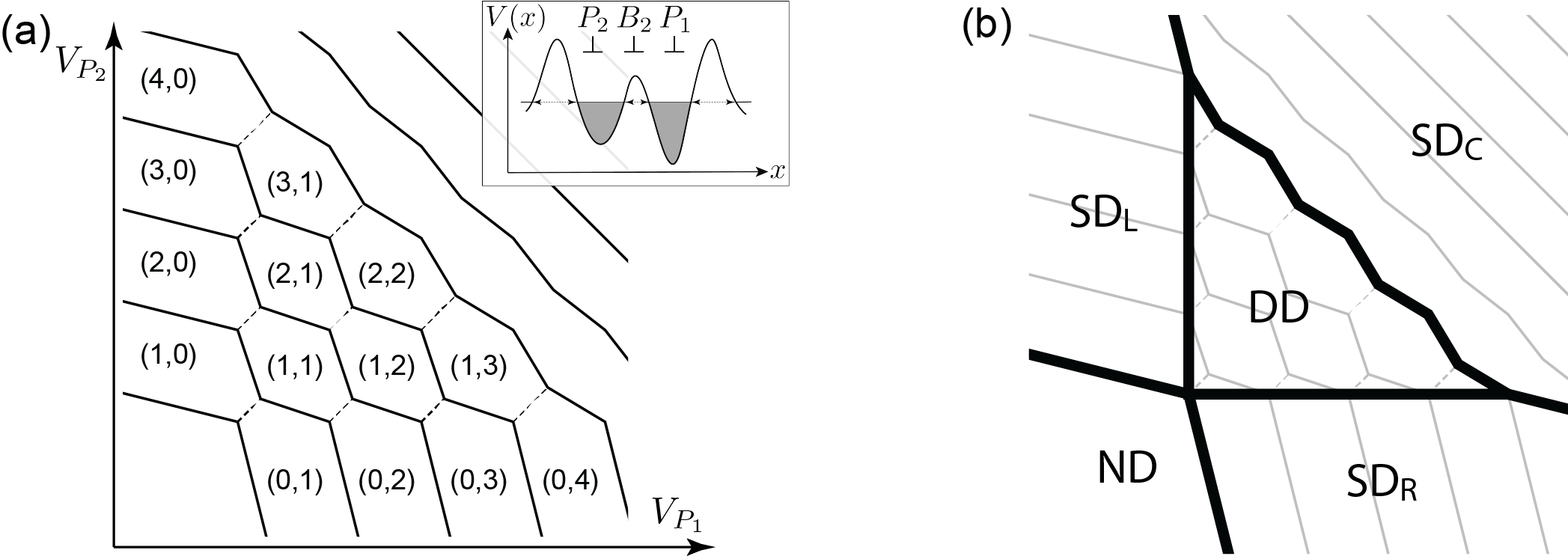
Figure 1: (a) A schematic charge stability diagram, with visually evident tiling of the $V_{P_{1}}$-$V_{P_{2}}$ plane by irregular polygons. The $(m,n)$ labels indicate the QD charge configuration. As the plunger values are simultaneously increased, the two QDs merge as the electrons cease to localize on a single QD. The inset shows the potential landscape of the double-QD system. (b) The state map dividing the $P_{1}$-$P_{2}$ configuration space into five distinct global state domains, with ND indicating the region in the $P_{1}$-$P_{2}$ plane where no QDs formed, SD_L, SD_C, and SD_R denoting the left, central, and right single QD, respectively, and DD denoting the double-QD state.

Methods

In semiconductor QD-based quantum computing, the aim is to confine electrons in potential wells using precise electrostatic controls. These come in the form of plunger gates, which create potential wells, and barrier gates, which create electrostatic barriers; see the inset in Fig. 1(a). The confinement wells, when filled, become QDs; in the case of two such dots, typically a total of five gates – two plungers and three barriers – are used to electrostatically confine electrons and separate them from the environment and each other. With fixed barrier potentials, the plunger potentials $V_{P_{1}}$, $V_{P_{2}}$ can vary through a dynamic range defining the relevant configuration space. The total charge within the device can be measured using a quantum point contact or a single electron transistor [35]. The discrete nature of the electrons leads to a charge stability diagram in which regions of the device’s $V_{P_{1}}$-$V_{P_{2}}$ configuration space show stable ground-state charge configurations. See Fig. 1(a) for an idealized depiction of a charge stability diagram, Fig. 2(a) for an example of a noisy simulated scan, and Fig. 2(d) a real-world example.

QD auto-annotator algorithm overview

Due to the assumed weak tunnel coupling of QDs, the ground state charge configurations of the QD device can be described via the constant interaction model in which the possible charge configurations form convex polytopes [36, 37, 38]. A schematic of a 2D charge stability diagram with visually evident irregular tiling and charge configuration of each tile is shown in Fig. 1(a). The various polytopes’ shape, size, and orientation provide information about the discrete states they represent. The goal of the QD auto-annotator is to create state-level decomposition of the configuration space into domains capturing the possible states of the device based on the polytopal tiling. The QD auto-annotator uses a classical algorithm to create a model of each polytope. Polytopes with similar characteristics cluster together, allowing the subdivision of the charge stability diagrams into distinct global state domains, where the system exhibits a consistent behavior. A sample division of a configuration space into a no QD (ND), a left, central, and right single-QD (SD_L, SD_C, and SD_R, respectively), and double-QD (DD) state subdivisions is depicted in Fig. 1(b).

The QD auto-annotator algorithm has three distinct phases: model building, statistical inferencing, and global state determination. The model building phase uses the fingerprinting method [39, 40] to collect the information necessary to build discrete polygonal models. In the statistical inferencing phase, gross features of the polygons, i.e., orientation, interior angles, number of edges, etc., are used to group the polygons into classes. Because noise effects can distort polygon models in unpredictable ways, this phase also makes noisiness and reliability determinations to differentiate between reliable and unreliable models. The final global state determination phase divides the scan into global state domains, by first using the grouping results from the statistical inferencing phase, and then creating models of the global domains based on underlying physical principles. Typically, the DD state grades into the SD_L, SD_C, or SD_R state without any sharp boundary as the interdot coupling between the QDs increases [38]. To accommodate this, the QD auto-annotator algorithm examines each polygon individually and applies explicit external rules based on electron confinement physics [38] to assign a probability that a given polygon belongs to the DD or SD_C state.

Given that the fingerprinting method is error-prone in the presence of noise, the QD auto-annotator relies on high levels of measurement redundancy, which is easy to accommodate in the offline setting, i.e., when used to analyze pre-measured scans as opposed to data acquired in a real-time, along with certain statistical methods to obtain reliable state labeling.

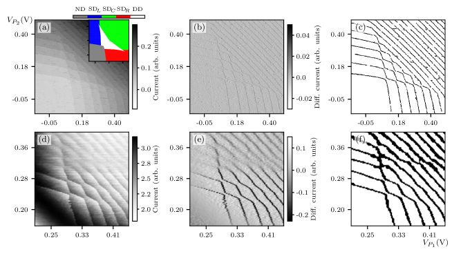
Figure 2: A sample 2D map (a) generated with the QD simulator [30] and (d) acquired experimentally. The numerical derivative of the measurement showing the irregular polytope tiling of the 2D space for (b) the simulated measurement depicted in (a) and (e) the experimental data depicted in (d). The inset in (a) shows the ground truth state labels, created by the simulation. The binary threshold map that the QD auto-annotator requires as input for (c) the simulated measurement depicted in (a) and (f) the experimental data depicted in (d).

Simulated and experimental data overview

An example of a simulated QD device measurement, analogous to ones typically acquired in the laboratory, its numerical derivative showing the polygonal tiling, and the corresponding threshold map are shown in Fig. 2(a), Fig. 2(b), and Fig. 2(c), respectively. Similar depictions for an experimentally acquired scan from the QFlow 2.0 dataset are shown in Fig. 2(d), Fig. 2(e), and Fig. 2(f), respectively. An inset in Fig. 2(a) shows the state map (available only for simulated data) corresponding to a measurement shown in Fig. 2(a). The $x$ and $y$ axes represent a subset of parameters changed in the experiments (here, the plunger gate voltages controlling the formation of the QDs, see inset in Fig. 1(a)), and the curves represent the device response to a change in QD electron occupation.

The simulated data used in this work is generated using a physics-based simulator of QD devices [30]. Each simulated measurement is stored as a separate file that includes the physical parameters defining the QD device, the measurement range for each axis, the transport and charge sensor measurement, a ground-truth global state map, a ground state charge configuration map for the SD_L, SD_C, SD_R, and DD states, and the simulated noise level. The experimental data files contain the charge sensor data, the voltage range for each axis over which the measurement was performed, as well as information about the device used in the measurement.

Data preparation module

The raw charge stability diagrams from both simulated and experimentally acquired measurements represent the QD device response to a change of a particular parameter (or parameters), with the value at each point (pixel) indicating the purported total charge on the device. The QD auto-annotator requires as an input a binarized version of the charge stability diagram which we call a threshold map. Regions where the charge configuration remains unchanged are labeled in the threshold map as $0$ while pixels capturing the device response to a change in electron occupation, i.e., a voltage configuration where an electron moves into or out of the QD, are labeled as $1$. An example of a binary threshold map for the simulated and experimentally acquired measurements shown in Fig. 2(a) and Fig. 2(d) are shown in Fig. 2(c) and Fig. 2(f), respectively.

Both simulated and experimental charge stability diagrams can be noisy and filled with numerous artifacts, some of which can be theoretically accounted for and some of which are simply stochastic. Moreover, the measurement characteristics can vary widely between the different types and designs of QD devices. The data denoising and binarization involve human input in the form of choosing local gradient thresholds and tuning gradient filters. For high-noise data, additional correlational strategies are employed to ameliorate labeling errors. The preprocessing of data is carried out outside of the QD auto-annotator.

Model-building module

The first step of the QD auto-annotator is the creation of polygon models from the threshold map. The primary tool here is fingerprinting.

Definition 1 (Point fingerprint in 2D)

Let $x_{o}$ be an observation point sampled within a 2D charge stability diagram. A point fingerprint $\mathcal{F}_{x_{o}}$ at an observation point $x_{o}$ is a list of weighted distances from that point to the nearest charge transition line along evenly spaced one-dimensional (1D) measurements called rays [39, 40].

The idea of using fingerprints to classify simple high-dimensional geometrical structures was first proposed in the context of cost-effective calibration of QD devices [39, 19, 40]. However, while for ML-driven classification purposes the qualitative information about the boundaries defining the polytopes suffices, capturing the smooth transition between the states for the purpose of labeling the 2D charge stability diagrams requires full modeling of the structures of interest. In addition to fingerprints the model-building module requires also information about the orientation of the respective rays to determine the position of the terminal points, i.e., points in the 2D configuration space where rays cross transition lines. We call the fingerprint combined with a vector of ray orientations an extended point fingerprint.

Localizing observation points

The model-building process starts with a selection of observation points from which the extended fingerprints will be measured. Ideally, each observation point should be located at the center of a polytopal domain. This desired arrangement of the centralized observation points is achieved through an iterative process. Starting with a selection of initial observation points on a dense hexagonal grid with points spaced every four pixels, an extended fingerprint is measured at each point and then fitted to rough star-shaped polygon models [41]. The centers of mass of the resulting models become new observation points, see Fig. 3(a). Iterating, this causes points to cluster at polygon centers in those regions where convex polygons are captured in the threshold map, see Fig. 3(b). In regions where the transition map has parallel or near-parallel lines, observation points do not cluster at center points, but rather along median lines. A simple process of pruning reduces the initial very large number of points to a relative few: if the distance between two observation points is less than the interior radius of either of the polygons they define, the two points are combined into a single point at the midpoint between them. The process continues until the locations of the observation points stabilize.

Fingerprinting charge stability diagram

Having found properly distributed observation points, the next step in the QD auto-annotator algorithm is to measure extended fingerprints at these points and build the final convex polygon models from each fingerprint, see Fig. 3(c). In noise-free settings, this is a completely straightforward process. However, the data binarization may give rise to three types of errors: (i) noise artifacts misidentified as indicators of charge transitions; (ii) transition lines with gaps when the thresholding detects no charge transition where a transition should be present; and (iii) stochastic imprecisions in transition line locations. The first two types of errors may severely hinder the model-building attempt and thus must be identified by the algorithm. In brief, some rays will strike a noise pixel before striking a transition line resulting in a ray that is too short, while others might miss a transition that should be present resulting in a ray that is too long. A dense sampling of rays allows relatively easy identification of individual or small clusters of ray anomalies, and additional checks for deviations from convexity allow the identification of larger groups of anomalous rays. All anomalous rays are removed from the analysis prior to modeling, see Fig. 3(d).

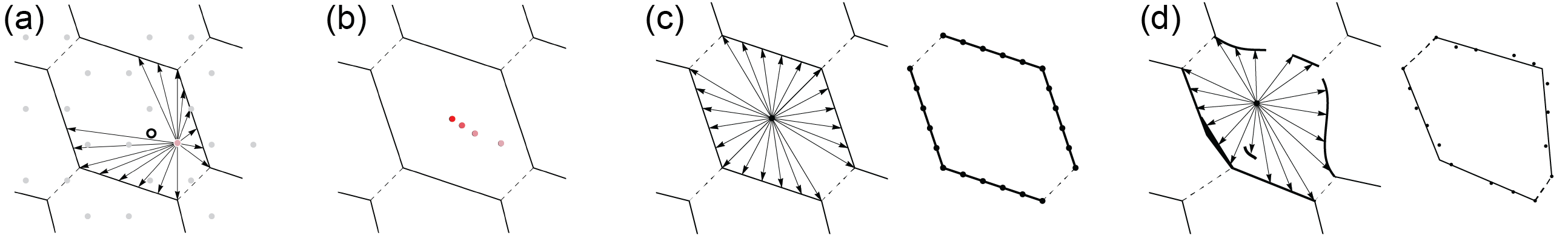
Figure 3: The polygon model creation. (a) A preview of a fingerprint measurement from a sample point (shown in pink) from the initial grid of observation points. A preview of the initial grid of sampled points is shown in gray. (b) A series of consecutive observation points selected by the model-building module with the intensity of the color indicating the progress of the algorithm. (c) Model creation for a nearly ideal polygon (right) and the resulting polygon (left). (d) A corrected set of rays for a noisy model a polygon (right) and the resulting polygon model (left).

The imprecise positioning of the charge transitions is dealt with by using best-fit techniques to model extended fingerprint terminal points with line segments. While Gaussian best-fit methods are often used in such situations, modeling with a Gaussian cost function is unstable and even in reasonable cases may produce poor fits with data, see, e.g., the Simpson’s paradox [42, 43, 44]. Instead, we use the much more stable normalized $\ell^{2}$ Hausdorff distance to measure the fidelity of line segments to groupings of terminal points [45].

Definition 2 (Normalized Hausdorff distance)

Let $A$ and $B$ be nonempty, finite sets of points within a metric space with metric $\rho$. The normalized $\ell^{2}$ Hausdorff distance is

$$\rho_{H}(A,\,B)\;=\;\left(\textstyle\frac{1}{2}\mathcal{D}(A;B)^{2}\,+\,\frac{1}{2}\mathcal{D}(B;A)^{2}\right)^{\frac{1}{2}},$$ (1)

where $\mathcal{D}(A;B)$ is the $\ell^{2}$-deviation of $A$ with respect to $B$ defined as

$$\mathcal{D}(A;B)=\bigg{(}\frac{1}{|A|\,\text{diam}(A)^{2}}\sum_{x\in{A}}\text{dist}(x,B)^{2}\bigg{)}^{\frac{1}{2}},$$ (2)

with $\text{dist}(x,B)=\min\left\{\rho(x,\,y)\;\big{|}\;y\in{}B\right\}$, $|A|$ denoting the cardinality of $A$, and $\text{diam}(A)=\sup\left\{\text{dist}(x,\,y)\;\big{|}\;x,y\in{}A\right\}$ denoting the diameter of $A$.

The set function $\mathcal{D}$ is not symmetric in $A$ and $B$. Intuitively, $\mathcal{D}$ measures how far, in a root mean square sense, a typical point of $A$ lies from the nearest point of $B$. For example, $A\subseteq{}B$ implies $\mathcal{D}(A;B)=0$ but says nothing about $\mathcal{D}(B;A)$. $\mathcal{D}$ is unitless and scale-invariant. The set function $\rho_{H}$, on the other hand, is symmetric in $A$ and $B$ and $\rho_{H}(A,B)=0$ if and only if $A$ and $B$ are the same set.

Fitting and modeling

The next phase of the model-building module involves fitting each of the extended fingerprints to a model. There are four kinds of polygons possible in a double-QD charge stability diagram: hexagons with two missing edges (representing mainly the DD state), pentagons with one missing edge (representing the SD_L and SD_R states), quadrilaterals (representing the SD_C state), and triangles (representing the ND state). Any missing edge in a model, should any exist, is called an aperture. This choice of geometric models is informed by the constant interaction model of double-QD systems described in the Labeling Double-dot states section. Each model is determined by a finite number of parameters that include the model’s vertex points and the presence of apertures. Every choice of parameters determines a new polygonal model, which is then discretized. Letting this discretization be the set $A$ and the fingerprint endpoints be the set $B$, we evaluate the $\ell^{2}$ distance function $\rho_{H}(A,B)$. Interpreting this as a cost function, we then search for model parameters that minimize this cost.

If the polygon has $n$ vertices (for the double-QD device $n$ is $4$, $5$, or $6$), then $\rho_{H}$ must be minimized in a $2n$ dimensional configuration space. This search is carried out in two steps: a rough search and a fine search. In the rough search phase, all terminal points for a given extended fingerprint are ordered sequentially and each possible subset of $n$ sequential points is used to build a polygon model. We then find the smallest value of $\rho_{H}$ among the resulting models. For $N$ terminal points, this means testing ${{N}\choose{n}}=\frac{N!}{(N-n)!n!}$ possible models. When $n$ is small and $N\gg n$ this is larger than $(N-n)^{n}/n!$, which can become computationally prohibitive for large $N$. Thus, we employ several mitigation strategies to reduce the number of models that need to be checked. For quadrilateral models, we bring the number of models to test down to about $2\cdot(N/2)^{2}$ by requiring that two of its vertices are diameter points of the fingerprint. When testing pentagonal or hexagonal models, we first search for gaps in the termination points and then force model apertures to span one or more of these gaps. If the number of gaps is $M$, this reduces the search to $M\cdot{}O(N^{2})$ models in the pentagonal case and ${{M}\choose{2}}\cdot{}O(N^{2})$ in the hexagonal case.

The second phase, the fine search, begins with the model selected in the rough search. Because the search space in the rough-fitting phase was restricted to only checking terminal points, it is possible that nearby points not included in the extended fingerprint might result in a substantially better fit. As noted earlier, $\rho_{H}$ can be considered a function on $2n$-dimensional space. To optimize the fit we employ the discrete gradient flow method on the gradient of $\rho_{H}$ in this space. At each step in the flow the model’s vertex points can move at most one pixel from their previous location. This constraint prevents oscillatory behavior. The number of steps necessary for convergence depends on the internal characteristics of the extended fingerprint, e.g., the size of the largest gaps between terminal points. In practice, we observe convergence in no more than 6 steps except for polygons in very noisy regions where this number can get larger. The fine search is computationally less demanding than the rough search, as gradients can be computed in polynomial time with respect to the number of polygon parameters. In our case, the computation cost scales as $N\cdot{}O(n)$ where $N$ is the number of fingerprint terminal points. Since in our application $n\ll N$, this is significantly better than the $O(N^{2})$ computation time for the rough search after improvements.

The result of the fine search is a polygon model for each extended fingerprint that locally minimizes the $\rho_{H}$ cost function. The polygon creation process produces a polygonal tiling of the threshold map. Since the polygons are modeled independently, the resulting models may partly overlap one another and various-sized gaps between polygons may occur at this stage.

Such inaccuracies are most likely to occur in regions where the centralization algorithm is semi-stable, which happens when transition lines become roughly parallel (the CD area) and in the transitional area for high levels of noise. To fine-tune the proper tiling of the 2D map and to derive the final state labels we invoke methods of statistical inferencing.

Statistical inferencing module

The polygon models provide an assemblage of discrete information about the underlying charge stability diagrams. From this information we gather statistics, isolate relevant features of the threshold map, and identify and filter noise that has come through the filtering mechanisms to this point.

Noise statistics and filtering

The first relevant feature the QD auto-annotator collects statistics on is how well the polygon models fit their respective extended fingerprints. The fit is measured using the normalized $\ell^{2}$ Hausdorff distance $\rho_{H}$ discussed in the previous section [45].

Definition 3 (Model error at $x_{o}$)

Let $\mathcal{F}_{x_{o}}$ be an extended fingerprint from an observation point $x_{o}$, $A$ denote its set of terminal points and $B$ denote the set of all points on its polygon model except those that lie on any aperture segments. We define the model error at an observation point $x_{o}$ as $\mathcal{E}(x_{o})=\rho_{H}(A,B)$.

After the polygon around each observation point $x_{o}$ receives the error score $\mathcal{E}(x_{o})$, the scores are analyzed collectively to determine their statistical spread. Empirically, low-noise scans have model errors tightly clustered near $0$, see Fig. 3(c), while high-noise scans show large deviations, see Fig. 3(d). If a polygon model’s $\mathcal{E}(x_{o})$ lies more than $2$ standard deviations away from the mean, it is discarded. This creates gaps in the tiling of the threshold map which are overcome through statistical methods.

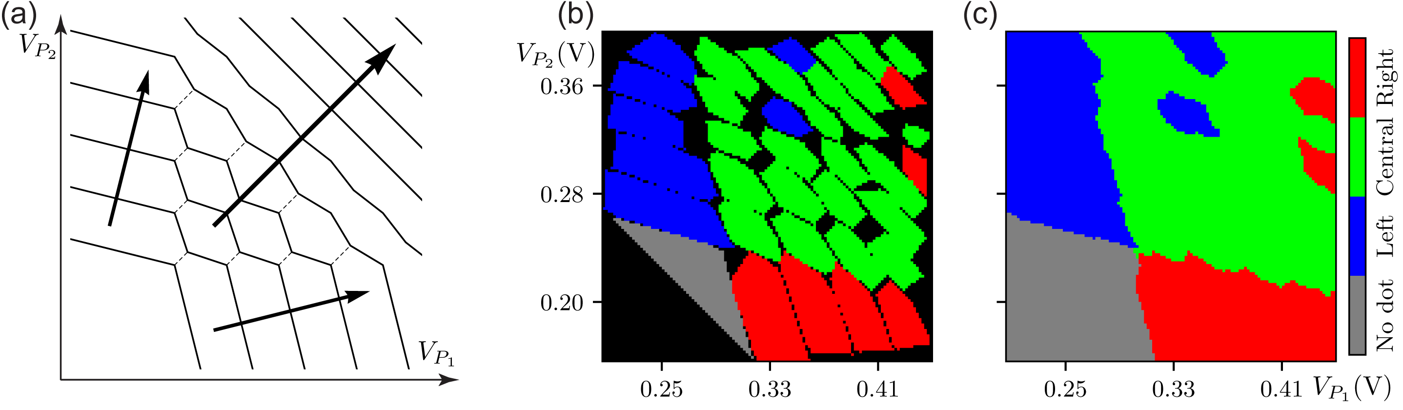
Figure 4: (a) The depiction of the characteristic left, center, and right dominant directions of the $P_{1}$-$P_{2}$ configuration space. (b) Fingerprint-modeled polygons for the device shown in Fig. 2(d), showing overlaps and gaps, and some misidentifications caused by noise and boundary effects. Overlaps are resolved by assigning to each contested point the observation point that it is closest to. Gaps are resolved by the expansion method described in the text. (c) The “filled in” map. In (b) and (c) the red, green, and blue colors indicate left, central, and right orientation, respectively. The gray color indicates the ND domain and the black color indicates pixels were not assigned to any polygon during the modeling phase.

Establishing directionality: Heat flow clustering

After the polygons have been created and filtered based on the fit quality, the remaining models are used to create the gross characteristics of the threshold map. Polygon models must be clustered by their orientation into the scan’s dominant directions, which must also be detected. For a double-QD there are three dominant directions: left, right, and center corresponding to the left, right, and combined double and central QD state, respectively; see Fig. 4(a). The QD auto-annotator does not assume the existence of all directions in a given scan. Rather, the system is designed to automatically recognize which directions are present and which states need to be characterized.

The dominant directions present in the threshold map are determined through clustering of polygon orientations defined by the unit normal to the median line through the model. The clustering is carried out by a custom heat flow clustering algorithm [46] rooted in the idea of persistence. The algorithm expands on techniques from the differencing potential method [47], in which a smooth kernel is chosen and convolved with the point locations, to produce a smooth potential field and the peaks of the potential field are then taken to be cluster centers, see Fig. 5. The challenge with the differencing potential method is in choosing a proper kernel since an effective choice requires foreknowledge of expected cluster widths as well as rough parity in the number of points within each cluster. Since this information is not available ahead of time, rather than relying on a single kernel, the heat flow clustering algorithm uses an ensemble of them. The idea is that intrinsic features of the data will manifest persistently through many kernel choices.

The algorithm works by selecting a static kernel $k(x)$ that resembles a Gaussian, and then scaling parabolically to obtain the time-dependent function $K(x,t)=k(x/\sqrt{t})/\sqrt{t}$; this parabolic scaling causes $K$ to imitate the classic 1D heat flow, particularly in that the kernel starts from nearly a $\delta$-function when $t$ is small and spreads through time while its $L^{1}$-norm remains constant. A selection of discrete times $\{t_{1},\dots,t_{N}\}$ is chosen and a clustering method, similar to a 1D version of the differencing potential clustering [47], is performed at each time $t_{i}$. The times $t_{1},\dots,t_{N}$ are chosen so that the smallest standard deviation and largest standard deviation have no chance of accurately resolving clusters. Then the $t_{i}$ are evenly spaced between, with $N=15$. Final cluster selections are arrived at when each point is assigned the cluster it most persistently belongs to. The heat flow clustering algorithm results in as few as one and as many as three cluster points which become the one, two, or three characteristic directions.

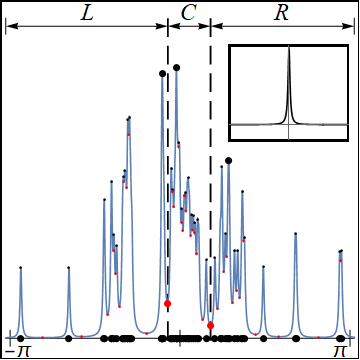
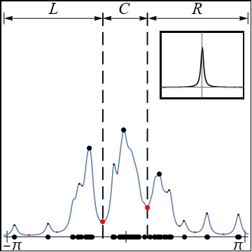
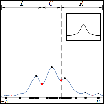
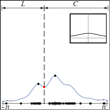
Figure 5: Various kernel choices in the heat flow clustering method. The $x$-axis parameterizes $\mathbb{S}^{1}$ and points are polygon orientations. Inset in each plot is the choice of kernel. Poor kernel choices lead to bad clustering, as shown in the first and last plots while correctly selected kernels lead to a potential showing clear and persistent clustering of points, as shown in the second and third plots. A majority of kernel selections will show the same or very similar clustering; then each point is assigned to the cluster it most persistently appears in. L, C, and R indicate left, center, and right orientation clusters, respectively.

Global state determination module

The final step of the QD auto-annotator is to create the domain decomposition based on the individual polygon identification and the statistical grouping. At this point, there may be errors or misidentifications in the polygon models, and the models themselves may overlap or have gaps between them, see Fig. 4(b). The fingerprinting architecture, used in the model-building module to model polygons, has the computationally valuable ability to easily create convex hulls and compute areas. In the global state determination module of the QD auto-annotator fingerprinting is used again, this time to model the global domains rather than individual polygons. The global state determination is performed in two phases: first the QD auto-annotator assigns each polygon to one of three orientation-based domains (left, central, and right). Then, in the second phase, the central domain is split into DD and SD_C states.

Remodeling

The polygon models obtained at this point might overlap and the overall tiling of the threshold map might contain gaps, as depicted in Fig. 4(b). Before the global state labels can be assigned the overlaps must be resolved and any existing gaps filled in, with each point in the scan assigned to a unique polygon. To eliminate the overlaps, the QD auto-annotator assigned each point claimed by two or more polygons to the nearest polygon center, as long as the direct line between the point and that center does not cross a transition line. To remove the gaps between polygons, the territory each polygon inhabits is expanded until all gaps are filled. The expansion process is carried out in two stages using a custom expansion method.

In the first stage, unassigned pixels adjacent to a classified polygon get absorbed by it as long as the line between the pixel and the centroid of the polygon it attaches to does not cross a transition line. This process is repeated to exhaustion, with the territory claimed by each polygon growing at a rate of at most one-pixel layer at each stage. Pixels belonging to transition lines in the threshold map are not considered at this stage. In the second run, the same process is performed, this time ignoring the transition lines and performing the expansion method without restriction until every pixel in the image is assigned to a polygon. For the ND state, the filling-in is carried out based on algebraic relation derived for the two short edges of the triangle where all points below those edges are automatically assigned to the ND class.

In the resulting filled-in map each pixel is classified as belonging to the ND, SD_L, SD_C, or SD_R state, though some polygons might at this point be misclassified, see Fig. 4(c). Moreover, at this stage of the analysis, the DD domain remains within the SD_C domain and will be separately identified later. The filled-in map is used to create the 4-state domain decomposition into ND, SD_L, SD_C, and SD_R states.

Labeling single-dot states

The QD auto-annotator classifies polygons into left, center, and right classes based on their orientations. However, due to fingerprinting and fitting errors as well as any number of noise factors and boundary effects, some polygons might be misclassified, as depicted in Fig. 4(c). To correct potential misclassifications, the QD auto-annotator performs a re-examination of all polygons within each class, with the underlying expectation being that the left-, center-, and right-class assigned polygons should mostly be contiguously grouped on the left, center, and right side of the scan, respectively. Individually misclassified polygons will likely be haphazardly distributed throughout the scan.

The re-examination is carried out on a per-class basis for the left and right orientation. For each class, a 0-or-1 map is created, with $1$ indicating a pixel attached to the class under consideration and $0$ indicating all alternative classes. To identify the most probable region of the scan to be assigned as the relevant domain, the algorithm first creates a convex hull of each contiguous grouping for a given class, then the area of each hull is computed and the region with the largest area is selected. Lastly, the selected convex hull is modeled with its own polygon using the same fingerprinting techniques as were used to create the smaller polygon models. This may result in assigning the fingerprint-modeled polygons to more than one domain. Points that belong to such multiple-domain polygons are used to determine the gradual transition between domains.

Labeling double-dot states

The center-dot region must be divided into DD and SD_C domains. However, the polygon orientation is insufficient to differentiate between the SD_C and DD states. Rather, the QD auto-annotator employs physical principles to make this determination. The transition between the SD_C and DD states is not sharp, so to label the scan we must be able to measure a grading between the states.

In the SD_C state, the valence electrons are not localized on either QD but form a pair that acts as an SD. In the DD state, in contrast, the electrons interact, but each is on a distinct QD[38]. In the charge stability diagram, the nature of the electron-electron coupling of the $(m,n)$ state is manifest by the shape of the $(m,n)$ polygonal cell. We interpret these shapes using the constant interaction model for coupled QDs [36, 38]. A quadrilateral cell indicates there is very little electrostatic coupling between the QDs: the central barrier is so high that the electrons are nearly non-interacting [see inset in Fig. 1(a)]. At the other end of the spectrum, indistinct cells indicate the electrons have merged into a charge-position multiplet: the barrier is so low that the electrons are no longer spatially separate. Hexagonal cell geometry indicates the barrier is large enough that the electrons are (mostly) spatially localized, but small enough that tunneling interactions are possible.

Figure 6: (a) The division of the hexagonal cell into an upper (above the centerline) and lower (below the centerline) polygon showing the cell roof (pink) and floor (green). (b) The polygonal cell’s dimensions in terms of physical quantities in the constant interaction model. Adapted from van der Wiel et al. [38].

To create a physically meaningful quantitative measure of the hexagon-ness of a cell, we divide each cell along its centerline [the dotted line in Fig. 6(a)] into an upper and lower cell (the regions above and below the dotted line, respectively). Then, we define the cell roof as the region above the dashed line of length $B$ in the upper cell in Fig. 6(a) and the cell floor as a corresponding region in the lower cell. After the polygon models have been built (see the Model-building module section), the following ratios are easily calculated:

$$U\;=\;\frac{\mathrm{area(roof)}}{\mathrm{area(upper\;cell)}}\quad\quad\mathrm{and}\quad\quad L\;=\;\frac{\mathrm{area(floor)}}{\mathrm{area(lower\;cell)}}.$$ (3)

We interpret these geometric ratios in terms of the constant capacitance model, with $B=[(\Delta{}V_{P_{1}})^{2}+(\Delta{}V_{P_{2}})^{2}]^{\frac{1}{2}}$, $\alpha=\frac{1}{2}[(\Delta{}V_{P_{1}}^{m})^{2}+(\Delta{}V_{P_{2}}^{m})^{2}]^{\frac{1}{2}}$, $\beta=-\alpha+\frac{\Delta{}V_{P_{1}}\,\Delta{}V_{P_{2}}}{B}$, and $\alpha,\beta\in[0,\frac{1}{2}B]$, where $\Delta{}V_{P_{i}}$ and $\Delta{}V_{P_{2}}^{m}$ denote the spacing between the charge transitions, see Fig. 6(b).

While in the idealized constant capacitance model $U=L$, in real-world devices, these ratios are equal only if device characteristics, such as cross-talk and stray capacitances, vary negligibly within the dynamic ranges of the plunger voltages. As this, in general, is not true, the values of $U$ and $L$ are expected to be different and are computed separately as

$$U,\,L\;=\;\frac{\frac{1}{2}\beta{}B}{\frac{1}{2}\beta{}B+\frac{1}{2}\alpha{}B}\;=\;1-\frac{1}{2}\frac{\sqrt{(\Delta{}V_{P_{1}}^{m})^{2}+(\Delta{}V_{P_{2}}^{m})^{2}}{}\,\sqrt{(\Delta{}V_{P_{1}})^{2}+(\Delta{}V_{P_{2}})^{2}}}{\Delta{}V_{P_{1}}\Delta{}V_{P_{2}}}.$$ (4)

In practice, the values of $\Delta{}V_{P_{1}}^{m}$, $\Delta{}V_{P_{2}}^{m}$ change with the absolute values of the gate voltages $V_{P_{1}}$ and $V_{P_{2}}$ and can vary substantially even within the same hexagon giving $U$ and $L$ measurably different values. In special cases, when $\Delta{}V_{P_{1}}\approx\Delta{}V_{P_{2}}\equiv\Delta{}V_{P}$ and $\Delta{}V_{P_{1}}^{m}\approx\Delta{}V_{P_{2}}^{m}\equiv\Delta{}V_{P}^{m}$, we can simplify Eq. (4) as

$$U\;\approx\;1-\frac{\Delta{}V_{P}^{m}}{\Delta{}V_{P}}\;\approx\;1-\frac{C_{M}}{C}\quad\quad\mathrm{and}\quad\quad L\;\approx\;1-\frac{\Delta{}V_{P}^{m}}{\Delta{}V_{P}}\;\approx\;1-\frac{C_{M}}{C}.$$ (5)

The range is $\Delta{}V_{P}^{m}\in[0,\Delta{}V_{g}]$ so that $U,L\in[0,1]$ with $0$ indicating a completely joined SD, $1$ indicating fully decoupled DD, and $U,L\in(0,1)$ indicating intermediate states of electron-electron coupling.

Although a quantitative grading between DD and SD states can be read off geometrically from the charge stability diagram, to give each polygon a specific label, a choice must be made as to appropriate cutoffs. Exactly where these cutoffs are located will depend to some extent on the application. The QD auto-annotator is fully customizable and can be adjusted depending on the research needs. From the area ratio we create the quantitative hexagon-ness score $\mathcal{H}$ for each polygon

$$\mathcal{H}\;=\;\begin{cases}\frac{1}{0.8}(U+L),&\text{if $0\leq\frac{1}{2}(U+L)\leq 0.4$}\\ 1,&\text{if $0.4<\frac{1}{2}(U+L)\leq 1$}\end{cases}$$ (6)

The $\mathcal{H}$ can be interpreted as the probability that a given polygon represents a DD versus SD state.

The final domain decomposition

The final domain decomposition involves the assignment of a vector-valued function from the pixel location $V_{i}=(x_{i},y_{i})$ within the charge stability diagram to a probability vector ${\bf p}(V_{i})=(p_{\rm ND},\,p_{{\rm SD}_{L}},\,p_{{\rm SD}_{C}},\,p_{{\rm SD}_{R}},\,p_{\rm DD})$ such that each component on vector ${\bf p}(V_{i})$ is non-negative and $p_{\rm ND}+p_{{\rm SD}_{L}}+p_{{\rm SD}_{C}}+p_{{\rm SD}_{R}}+p_{\rm DD}=1$ [17, 19]. The components of the vector ${\bf p}(V_{i})$ represent the probability that the point $V_{i}$ belongs to one of the five domains: $p_{\rm ND}$ is the probability the point $V_{i}$ is in the ND region, the $p_{{\rm SD}_{L}}$, $p_{{\rm SD}_{C}}$, and $p_{{\rm SD}_{R}}$ probabilities that point $V_{i}$ is in the left-, center-, and right-SD region, respectively, and $p_{\rm DD}$ is the probability that point $V_{i}$ is in the DD domain. The probabilities are assigned in three distinct phases: an initial sharp 4-domain probability assignment discussed in the Labeling single-dot states section (double-dot assignments not created yet), then the insertion of the double-dot graded probabilities based on the hexagon-ness score described in section Labeling double-dot states section, and finally the creation of a probability grading between the adjacent domains.

The initial 4-domain decomposition assigns to each point a state vector ${\bf p}^{(4)}(V_{i})=(p_{\rm ND},\,p_{{\rm SD}_{L}},\,p_{{\rm SD}_{C}},\,p_{{\rm SD}_{R}},\,0)$ where exactly one of $p_{\rm ND}$, $p_{{\rm SD}_{L}}$, $p_{{\rm SD}_{C}}$, and $p_{{\rm SD}_{R}}$ is $1$ and the others four components are $0$. After the polygonal modeling of the left-, right-, and ND domains described in the Labeling single-dot states section, every pixel is in a definite ND, LD, CD, or RD domain. However, the small fingerprint-defined polygons lying near the domain boundaries might overlap with two or more domains. When assigning the probability vectors, points inside polygons that were partially absorbed by one of the adjacent domains are resigned back to the original class based on the region its center-point lies within.

The second stage alters the polygons in the CD region by assigning to each polygon its DD probability. Using the score $\mathcal{H}$ given in Eq. (6), the state vector for points within this region is updated as ${\bf p}^{(5)}(V_{i})=(0,0,\,1-\mathcal{H},0,\,\mathcal{H})$. Outside of this region the state vector ${\bf p}^{(5)}(V_{i})={\bf p}^{(4)}(V_{i})$, with exactly one of $p_{\rm ND}$, $p_{{\rm SD}_{L}}$, and $p_{{\rm SD}_{R}}$ equal $1$ and the others components equal $0$.

Finally, in the third stage, the state vectors are probabilistically interpolated between the adjacent domains. The assignment of individual polygons to each state makes an artificially sharp and ridged boundary between the CD and LD or RD domains, see Fig. 4(c). At the same time, just as there is no completely sharp boundary between the CD and DD domains, there is no completely sharp distinction between the CD and LD state or between the CD and RD state. The probability grading between the outer LD and RD domains and the laying between them CD and DD domains is determined geometrically. To do this, we observe that the individually labeled polygons drift into neighboring regions, as visible in Fig. 4(c), and we measure how far into that region they drift. We take these distances to be a standard deviation of the uncertainty of the region boundary. Then we convolve the 5-vector, with a local kernel having the width of this deviation. The result is a probability vector ${\bf p}(V_{i})$ that grades among the five regions based on the uncertainty in the boundary location. Figure 8(a) and  8(c) show the final domain decomposition for a sample noisy simulated device shown in Fig. 2(a) and a sample experimental scan shown in Fig. 2(d), respectively. Regions with confidence in the dominant label of at least $70\leavevmode\nobreak\ \%$ are represented as ringed areas in Fig. 7(b) for the simulated data and in Fig. 7(d) for the experimental scan. The gradual change in the color indicates transitional labeling.

Figure 7: Final probabilistic domain decomposition for (a) a sample noisy simulated device shown in Fig. 2(a) and (c) a sample experimental scan shown in Fig. 2(d) overlaying the charge sensor data. Regions with confidence in the dominant label of at least $70\leavevmode\nobreak\ \%$ represented as ringed areas for (b) the simulated data and (d) the experimental scan.

Technical Validation

In simulated settings, noise and sensor artifacts can be modeled and adjusted in a controlled fashion [31]. This allows for systematic validation of the QD auto-annotator performance for an increasingly degrading data quality. To validate the auto-annotator, we use a set of 7 qualitatively distinct simulated double-QD devices with varying levels of noise [20, 25]. The noise levels used in these tests are varied around a reference level extracted from the experimental data [20]. For simplicity, the reference noise is denoted as 1.00. For each simulated device we use 16 noise levels ranging from $0.00$ (noiseless data) to $5.00$. In addition, we test the performance of the QD auto-annotator on a set of 9 large experimental scans from the QFlow 2.0 dataset [29].

Validation with simulated data

Figure 8: The performance of the QD auto-annotator on a per-domain basis for different noise levels for the 7 simulated devices. The inset shows an overall performance across all domains and all devices for each noise level.

Using the ground truth labels assigned at a pixel level during simulations and the QD auto-annotator labels we can quantify both the overall per-device agreement between labels as well as the per-class performance. The ground truth labels for the simulated data, $\mathcal{L}(V_{i})$, are represented as one-hot vectors, with the hot component indicating the assigned state. The QD auto-annotator algorithm provides a map where each pixel is assigned a probability vector ${\bf p}(V_{i})$. To quantify the overall performance, we compare these two vectors at each point within each simulated scan. Pixels for which the QD auto-annotator shows an agreement with ground truth at least $70\leavevmode\nobreak\ \%$ are flagged as correct. Otherwise, they get an incorrect flag. We observe an overall state assignment agreement at around $97\leavevmode\nobreak\ \%$ when averaged over all devices for noise levels up to $3.00$, see the inset in Fig. 8. Once the noise level surpasses $3.00$, the agreement deteriorates slightly to $95.6(3.3)\leavevmode\nobreak\ \%$ at noise level $4.00$ and $93.3(2.8)\leavevmode\nobreak\ \%$ at noise level $5.00$. For comparison, the performance of a QD charge tuning algorithm proposed recently [20] begins to decline at noise level $2.00$.

We then compute the proportion of correct pixel assignments to the total number of pixels in each of the five domain regions, as determined by the ground truth labels. Figure 8 shows the performance of the QD auto-annotator on a per-domain basis for each noise level for the 7 simulated devices. The ND, SD_L, and SD_R state identifications remain almost perfectly robust up to the highest considered noise level. The CD_L state shows a slight decay in performance at higher noise levels (at around noise level $3.00$). The DD state assignment is the most fragile and breaks down once the simulated noise levels surpass $3.50$.

The statistical determination, error mitigation, and data redundancy ensure stable state assignments for ND, SD_L, and SD_R. Since the domains in the charge stability diagrams decomposition are complementary, the high and consistent performance in classifying these three domains naturally translates on a comparable performance in determining the combined SD_R and $DD$ domain (the central orientation region). The QD auto-annotator’s sub-statistical boundary determination between SD_R and $DD$ domains results in performance degradation at higher noise levels.

The boundary between the SD_R and $DD$ regions is determined by a series of measurements on individual polygons quantifying their hexagon-ness, see Eq. (4) and Eq. (6). Because this process relies on measurements taken on individual polygons, it contains no redundancy or statistical error-checking which makes the SD_R and $DD$ state assignment more sensitive to noise. However, despite this limitation, the SD_R and $DD$ state assignments remain quite robust up to a fairly high level of noise, as can be seen in Fig. 8.

Validation with experimental data

For the experimental data, the ground truth labels are not available. It is thus not possible to perform large-scale quantitative validation of the QD auto-annotator performance. Thus, when assessing the outputs of the algorithm for experimental data we focus on the qualitative features resulting from the assigned labels. In particular, we focus on the overall locations of the individual states within the 2D configuration space, such as the ND state in the bottom left corner or the SD_L and SD_R states on the top-left and bottom-right sides, respectively. We also consider the agreement between the charge transition lines geometry, e.g., horizontal or vertical parallel lines, and the assigned global state label, e.g., the SD_R or SD_L state. Finally, we look at the correctness of the transitional regions, i.e., DD state blending into SD_L as $V_{P_{1}}(V)$ decreases, into SD_R as $V_{P_{2}}(V)$ decreases, and into SD_C as $V_{P_{1}}(V)$ and $V_{P_{2}}(V)$ increase.

The output of the QD auto-annotator is a 2D map with a label at each point indicating the probabilistic assignment of the five possible states. A sample probabilistic domain decomposition for the experimental scan shown in Fig. 2(d) is depicted in Fig. 7(c). To ease the analysis, the state labels are shown overlaying the original scan. Figure 7 highlights in the configuration space regions where the label confidence surpasses $70\leavevmode\nobreak\ \%$ as well as regions where the labels indicate a transition between states (i.e., all components of the probability vector ${\bf p}(V_{i})$ are less than $0.7$). A visual inspection of these two images confirms a high level of agreement between the QD auto-annotator assigned labels and the human interaction. To further validate the quality of the domain decomposition returned by the QD auto-annotator we consulted with two external experts – one working in academia and one in the industry. Both experts are experimentalists with long experience in the semiconductor QDs domain. The received feedback further confirms the high level of agreement between the automatically generated labels and how the experts thought they would manually label the data

Data Records

The QFlow 2.0 dataset [29] is hosted and freely available at data.nist.gov. Data representing the seven simulated QD devices as well as labels for all experimental scans supporting the findings of this study are added to the database.

The reference (i.e., noiseless) simulated test QD devices used in this work are stored as separate NumPy files in the compressed simulated\sim_test folder. The name of each simulated file indicates the simulated device configuration and the noise level, e.g., 10nmGatePitch_SmallSlopeScreening_NoiseLevel0.20.npy. The experimental data are named as exp_large_$xx$.npy, where $xx$ are consecutive numbers between $0$ and $12$. The taxonomy of the files is presented in Table 1. The Item field indicates the dictionary key, the Description field indicates the dictionary value, and the Noiseless data, Noisy data, and Experimental data columns indicate whether or not a given item exists for a given data type.

Item	Description	Noiseless	Noisy	Experimental
sensor	Simulated data: The output of the charge sensor evaluated as the Coulomb potential at the sensor location (with simulated noise added if in the noisy sensor data). Experimental data: the charge sensor data (in amperes).	+	+	+
V_P1_vec	A voltage range for the first plunger ($V_{P_{1}}$).	+	+	+
V_P2_vec	A voltage range for the second plunger ($V_{P_{2}}$).	+	+	+
state	The label determining the state of the device at each point, distinguishing between ND (0), SDL (0.5), SDC (1), SDR (1.5), and a DD (2)	+	+	–
charge	The information about the number of charges on each QD (with a default value 0 for ND state).	+	+	–
noise_level	The level of the simulated noise.	+	+	–
mask	The binary threshold map.	+	+	+
qda2_vec	The probabilistic state labels returned by the QD auto-annotator at each point.	+	+	+
conf_ring	The $70\leavevmode\nobreak\ \%$ confidence ring indication the dominant state labels.	+	+	+

Table 1: The taxonomy of the data files added to the QFlow 2.0 dataset. The first column identifies each item in the respective files (expressed as keys in the relevant Python dictionary). The second column provides the description of each item. The last three columns indicate whether or not a given item exists for a given data type.

Usage Notes

The QD auto-annotator is a critical step in a proposed public-private-academic partnership intended to produce a data-sharing system for the QD community [24]. The lack of such sharing partnerships has been recognized as a hindrance to development within this field. Establishing a comprehensive and reliable reference database of labeled experimental data is essential for the development of automation tools for the characterization and control of QD devices. The QD auto-annotator is the first step on the path to establishing such a standardized database.

The QD auto-annotator enables systematic processing and labeling of experimentally acquired charge stability diagrams. The validation of the algorithm’s performance using simulated data confirms that it can reliably label data with noise levels surpassing what is typically observed in experiments. However, as we discussed in the Data preparation module section, the QD auto-annotator requires a binarized version of the charge stability diagram as input. At the same time, the thresholding module relies at present on human input which presents a bottleneck to large-scale deployment of the QD auto-annotator. While we are actively developing an algorithm for fully automated binarization of the experimental charge stability diagrams, this effort is impeded by a lack of openly available moderate- and poor-quality experimental data given the still prevalent practice in the QD community to “make data available only upon “reasonable request,” or to not share it at all” [24].

The success of the current project is aimed at providing concrete, mutual benefits to data sharing. The value-added proposition, described here, is the automatic processing and labeling of datasets that the QD auto-annotator makes possible at scale. Once the automated thresholding module is completed, a simple, web-based interface for uploading and processing QD data using the QD auto-annotator will become available. In the meantime, access to the QD auto-annotator will be restricted to users interested in sharing their data to aid the development of data binarization methods. In addition, all labeled data will be systematically added to the QFlow 2.0 [29] database.

Code availability

The dataset used in this work, QFlow 2.0 [29], is stored at data.nist.gov. The size of the datasets is over $13$ GB (compressed), which includes $13.4$ GB of simulated data and $15.8$ MB of experimental data. The QFlow 2.0 is provided subject to open-access licensing for researchers globally. The code used to generate the QFlow 2.0 is being prepared for public release together with instructions for reproduction of the dataset [48]. An access to the functionality provided by the QD auto-annotator will be provided via a web-based interface. In addition, all new data analyzed via the web-based interface will be added to the QFlow 2.0 database.

Author contributions statement

J.P.Z. developed the concept of using principled approaches to label experimental data. J.P.Z. and B.W. formalized the idea of using ray-based measurement to label device scans. B.W. wrote the code implementing all modules proposed in this work, including several custom algorithms. B.W. and J.P.Z. performed the numerical experiments and data analysis, refined the performance metrics, and wrote the manuscript.

Competing interests

The authors declare they have no conflict of interest.

References

- [1] Zwanenburg, F. A. et al. Silicon quantum electronics. \JournalTitleRev. Mod. Phys. 85, 961–1019, 10.1103/RevModPhys.85.961 (2013).
- [2] Petta, J. R. et al. Coherent manipulation of coupled electron spins in semiconductor quantum dots. \JournalTitleScience 309, 2180–2184, 10.1126/science.1116955 (2005).
- [3] Koppens, F. H. L. et al. Driven coherent oscillations of a single electron spin in a quantum dot. \JournalTitleNature 442, 766–771, 10.1038/nature05065 (2006).
- [4] Medford, J. et al. Quantum-dot-based resonant exchange qubit. \JournalTitlePhys. Rev. Lett. 111, 050501, 10.1103/PhysRevLett.111.050501 (2013).
- [5] Kim, D. et al. High-fidelity resonant gating of a silicon-based quantum dot hybrid qubit. \JournalTitlenpj Quantum Inf. 1, 15004 (2015).
- [6] Barthel, C., Reilly, D. J., Marcus, C. M., Hanson, M. P. & Gossard, A. C. Rapid single-shot measurement of a singlet-triplet qubit. \JournalTitlePhys. Rev. Lett. 103, 160503 (2009).
- [7] Veldhorst, M. et al. An addressable quantum dot qubit with fault-tolerant control-fidelity. \JournalTitleNat. Nanotechnol. 9, 981–985 (2014).
- [8] Kawakami, E. et al. Electrical control of a long-lived spin qubit in a Si/SiGe quantum dot. \JournalTitleNat. Nanotechnol. 9, 666–670 (2014).
- [9] Yoneda, J. et al. A quantum-dot spin qubit with coherence limited by charge noise and fidelity higher than 99.9%. \JournalTitleNature Nanotechnology 13, 102–106, 10.1038/s41565-017-0014-x (2018).
- [10] Vandersypen, L. M. K. & Eriksson, M. A. Quantum computing with semiconductor spins. \JournalTitlePhys. Today 72, 38–45, doi:10.1063/PT.3.4270 (2019).
- [11] Chanrion, E. et al. Charge detection in an array of CMOS quantum dots. \JournalTitlePhys. Rev. Appl. 14, 024066, 10.1103/PhysRevApplied.14.024066 (2020).
- [12] Zwerver, A. M. J. et al. Qubits made by advanced semiconductor manufacturing. \JournalTitleNat. Electron. 5, 184–190, 10.1038/s41928-022-00727-9 (2022).
- [13] Zwolak, J. P. & Taylor, J. M. Colloquium: Advances in automation of quantum dot devices control. \JournalTitleRev. Mod. Phys. 95, 011006, 10.1103/RevModPhys.95.011006 (2023).
- [14] Darulová, J. et al. Autonomous tuning and charge-state detection of gate-defined quantum dots. \JournalTitlePhys. Rev. Appl. 13, 054005, 10.1103/PhysRevApplied.13.054005 (2020).
- [15] Baart, T. A., Eendebak, P. T., Reichl, C., Wegscheider, W. & Vandersypen, L. M. K. Computer-automated tuning of semiconductor double quantum dots into the single-electron regime. \JournalTitleAppl. Phys. Lett. 108, 213104, 10.1063/1.4952624 (2016).
- [16] Durrer, R. et al. Automated tuning of double quantum dots into specific charge states using neural networks. \JournalTitlePhys. Rev. Appl. 13, 054019, 10.1103/PhysRevApplied.13.054019 (2020).
- [17] Kalantre, S. S. et al. Machine learning techniques for state recognition and auto-tuning in quantum dots. \JournalTitlenpj Quantum Inf. 5, 1–10, 10.1038/s41534-018-0118-7 (2019).
- [18] Zwolak, J. P. et al. Autotuning of double-dot devices in situ with machine learning. \JournalTitlePhys. Rev. Appl. 13, 034075, 10.1103/PhysRevApplied.13.034075 (2020).
- [19] Zwolak, J. P. et al. Ray-based framework for state identification in quantum dot devices. \JournalTitlePRX Quantum 2, 020335, 10.1103/PRXQuantum.2.020335 (2021).
- [20] Ziegler, J. et al. Tuning arrays with rays: Physics-informed tuning of quantum dot charge states. \JournalTitlePhys. Rev. Appl. 20, 034067, 10.1103/PhysRevApplied.20.034067 (2023).
- [21] Czischek, S. et al. Miniaturizing neural networks for charge state autotuning in quantum dots. \JournalTitleMach. Learn.: Sci. Technol. 3, 015001, 10.1088/2632-2153/ac34db (2022).
- [22] Lapointe-Major, M. et al. Algorithm for automated tuning of a quantum dot into the single-electron regime. \JournalTitlePhys. Rev. B 102, 085301, 10.1103/PhysRevB.102.085301 (2020).
- [23] Botzem, T. et al. Tuning Methods for Semiconductor Spin Qubits. \JournalTitlePhys. Rev. Appl. 10, 054026, 10.1103/PhysRevApplied.10.054026 (2018).
- [24] Zwolak, J. P. et al. Data needs and challenges of quantum dot devices automation: Workshop report. \JournalTitle(in preparation) .
- [25] Ziegler, J. et al. Automated extraction of capacitive coupling for quantum dot systems. \JournalTitlePhys. Rev. Appl. 19, 054077, 10.1103/PhysRevApplied.19.054077 (2023).
- [26] Deng, L. The mnist database of handwritten digit images for machine learning research. \JournalTitleIEEE Signal Processing Magazine 29, 141–142 (2012).
- [27] Krizhevsky, A., Hinton, G. et al. Learning multiple layers of features from tiny images (2009). Toronto, ON, Canada.
- [28] Perrier, E., Youssry, A. & Ferrie, C. QDataSet, quantum datasets for machine learning. \JournalTitleSci. Data 9, 582, 10.1038/s41597-022-01639-1 (2022).
- [29] National Institute of Standards and Technology. Qflow 2.0: Quantum dot data for machine learning. Database: data.nist.gov, https://doi.org/10.18434/T4/1423788 (2022).
- [30] Zwolak, J. P., Kalantre, S. S., Wu, X., Ragole, S. & Taylor, J. M. QFlow lite dataset: A machine-learning approach to the charge states in quantum dot experiments. \JournalTitlePLoS ONE 13, e0205844, 10.1371/journal.pone.0205844 (2018).
- [31] Ziegler, J. et al. Toward robust autotuning of noisy quantum dot devices. \JournalTitlePhys. Rev. Appl. 17, 024069, 10.1103/PhysRevApplied.17.024069 (2022).
- [32] White House Office of Science and Technology Policy. Biden-harris administration announces new actions to advance open and equitable research. Fact Sheet, White House, Washington, DC (2023). Published 2023-01-11.
- [33] Existence and Use of Large Datasets To Address Research Questions for Characterization and Autonomous Tuning of Semiconductor Quantum Dot Devices. 88 Fed. Reg. 22409 (July 18, 2023). Accessed: 2023-10-17.
- [34] National Institute of Standards and Technology. Workshop on advances in automation of quantum dot devices control (2023).
- [35] Hanson, R., Kouwenhoven, L. P., Petta, J. R., Tarucha, S. & Vandersypen, L. M. K. Spins in few-electron quantum dots. \JournalTitleRev. Mod. Phys. 79, 1217–1265, 10.1103/RevModPhys.79.1217 (2007).
- [36] Beenakker, C. W. J. Theory of coulomb-blockade oscillations in the conductance of a quantum dot. \JournalTitlePhys. Rev. B 44, 1646–1656, 10.1103/PhysRevB.44.1646 (1991).
- [37] Schröer, D. et al. Electrostatically defined serial triple quantum dot charged with few electrons. \JournalTitlePhys. Rev. B 76, 075306, 10.1103/PhysRevB.76.075306 (2007).
- [38] van der Wiel, W. G. et al. Electron transport through double quantum dots. \JournalTitleRev. Mod. Phys. 75, 1–22, 10.1103/RevModPhys.75.1 (2002).
- [39] Zwolak, J. P., Kalantre, S. S., McJunkin, T., Weber, B. J. & Taylor, J. M. Ray-based classification framework for high-dimensional data. In Third Workshop on Machine Learning and the Physical Sciences (NeurIPS 2020), 1–7 (Vancouver, Canada, 2020). ArXiv:2010.00500.
- [40] Weber, B. J., Kalantre, S. S., McJunkin, T., Taylor, J. M. & Zwolak, J. P. Theoretical bounds on data requirements for the ray-based classification. \JournalTitleSN Comput. Sci. 3, 57, 10.1007/s42979-021-00921-0 (2022).
- [41] Singer, I. A. & Thorpe, J. A. Lecture Notes on Elementary Topology and Geometry. Undergraduate Texts in Mathematics (Springer-Verlag, New York, Heidelberg, Berlin, 1967).
- [42] Simpson, E. H. The interpretation of interaction in contingency tables. \JournalTitleJ. R. Stat. Soc. Series B Stat. Methodol. 13, 238–241 (1951).
- [43] Yule, G. U. Notes on the theory of association of attributes in statistics. \JournalTitleBiometrika 2, 121–134, 10.1093/biomet/2.2.121 (1903).
- [44] Pearson Karl, L. & Leslie, B. Genetic (reproductive) selection: inheritance of fertility in man, and of fecundity in thoroughbred racehorses. \JournalTitlePhilos. Trans. R. Soc. Lond. Ser. A 192, 257–330, 10.1098/rsta.1899.0006 (1899).
- [45] Evans, L. C. & Gariepy, R. F. Measure theory and fine properties of functions (CRC press, 2015).
- [46] Weber, B. J. Information stability in the heat flow clustering. \JournalTitle(in preparation) .
- [47] Wang, S. et al. Clustering by differencing potential of data field. \JournalTitleComputing 100, 403–419 (2018).
- [48] Buterakos, D. i. Qflowsim: The quantum dot device simulator. \JournalTitle(in preparation) .
Acknowledgements
The views and conclusions contained in this paper are those of the authors and should not be interpreted as representing the official policies, either expressed or implied, of the U.S. Government. The U.S. Government is authorized to reproduce and distribute reprints for Government purposes notwithstanding any copyright noted herein. Any mention of equipment, instruments, software, or materials does not imply recommendation or endorsement by the National Institute of Standards and Technology.