Solving the Optimal Experiment Design Problem with Mixed-Integer Convex Methods

Abstract

We tackle the Optimal Experiment Design Problem, which consists of choosing experiments to run or observations to select from a finite set to estimate the parameters of a system. The objective is to maximize some measure of information gained about the system from the observations, leading to a convex integer optimization problem. We leverage Boscia.jl, a recent algorithmic framework, which is based on a nonlinear branch-and-bound algorithm with node relaxations solved to approximate optimality using Frank-Wolfe algorithms. One particular advantage of the method is its efficient utilization of the polytope formed by the original constraints which is preserved by the method, unlike alternative methods relying on epigraph-based formulations. We assess our method against both generic and specialized convex mixed-integer approaches. Computational results highlight the performance of our proposed method, especially on large and challenging instances.

1 Introduction

The Optimal Experiment Design Problem (OEDP) arises in statistical estimation and empirical studies in many applications areas from Engineering to Chemistry. For OEDP, we assume we have a matrix $A$ consisting of the rows $\mathbf{v}_{1},\allowbreak\dots,\mathbf{v}_{m}\in{\mathbb{R}}^{n}$ where each row represents an experiment. The ultimate aim is to fit a regression model:

$$\min_{\bm{\theta}\in{\mathbb{R}}^{m}}\|A\bm{\theta}-\mathbf{y}\|,$$ (1)

where $\mathbf{y}$ encodes the responses of the experiments and $\bm{\theta}$ are the parameters to be estimated. The set of parameters with size $n$ is assumed to be (significantly) smaller than the number of distinct experiments $m$. Furthermore, we assume that $A$ has full column rank, i.e. the vectors $\mathbf{v}_{1},\ldots,\mathbf{v}_{m}$ span ${\mathbb{R}}^{n}$.

The problem is running all experiments, potentially even multiple times to account for errors, is often not realistic because of time and cost constraints. Thus, OEDP deals with finding a subset of size $N$ of the experiments providing the “most information” about the experiment space (Pukelsheim, 2006; de Aguiar et al., 1995). The number of allowed experiments $N$ has to be larger than $n$ to allow the regression model in Equation 1 to be solved. It is, however, assumed to be less than $m$.

In Section 2, we investigate the necessary conditions for a function to be a valid and useful information measure. Every information function leads to a different criterion. In this paper, we focus on two popular criteria, namely the A-criterion and D-criterion, see Section 2.1.

In general, OEDP leads to a Mixed-Integer Non-Linear Problem (MINLP). There has been a lot of development in the last years in solving MINLP (Kronqvist et al., 2019). Nevertheless, the capabilities of current MINLP solvers are far away from their linear counterparts, the Mixed-Integer Problem (MIP) solvers (Bestuzheva et al., 2021), especially concerning the magnitude of the problems that can be handled. Therefore, instead of solving the actual MINLP, a continuous version of OEDP, called the Limit Problem, is often solved and the integer solution is created from the continuous solution by some form of rounding (Pukelsheim, 2006). This does not necessarily lead to optimal solutions, though, and the procedure is not always applicable to a given continuous solution either.

The goal of this paper is to compare the performance of different MINLP approaches for OEDP problems. A special focus is put on our newly proposed framework Boscia (Hendrych et al., 2023) which can solve larger instances and significantly outperforms the other examined approaches. Since it leverages a formulation and solution method that differ from other approaches, we establish the convergence of the Frank-Wolfe algorithm used for the continuous relaxations on the considered OEDP problems in Section 3. . The different solution methods are detailed in Section 4 and evaluation of the computational experiments can be found in Section 5.

1.0.1 Related Work

As mentioned, one established method of solution is the reduction to a simpler problem by removing the integer constraints and employing heuristics to generate an integer solution from the continuous solution. Recently, there have been more publications tackling the MINLP formulation of the Optimal Experiment Design Problem. These, however, concentrate on specific information measures, in particular the A-criterion, see (Nikolov et al., 2022; Ahipaşaoğlu, 2015), and the D-criterion, (Welch, 1982; Ponte et al., 2023; Li et al., 2022). The most general solution approach known to the authors was introduced in (Ahipaşaoğlu, 2021). It considers OEDP under matrix means which, in particular, includes the A-criterion and D-criterion. While the matrix means covers many information measures of interest, it still yields a restricting class of information functions. For example, the G-criterion and V-criterion are not included in this class of functions (de Aguiar et al., 1995). Our newly proposed framework Boscia only requires the information measures to be either $L$-smooth, i.e. the gradient is Lipschitz continuous, or generalized self-concordant, thereby covering a larger group of information functions. In addition, Boscia does not suppose any prior knowledge about the structure of the problem, being thus more flexible in terms of problem formulations. On the other hand, it is highly customizable, giving the user the ability to exploit the properties of their problems to speed up the solving process. An in-depth and unified theory for the Optimal Experiment Design Problem can be found in (Pukelsheim, 2006).

1.0.2 Contribution

Our contribution can be summarized as follows.

Unified view on experiment design formulations.

First, we propose a unified view of multiple experiment design formulations as the optimization of a nonlinear (not necessarily Lipschitz-smooth) information function over a truncated scaled probability simplex intersected with the set of integers. Unlike most other formulations that replace the nonlinear objective with nonlinear and/or conic constraints, we preserve the original structure of the problem. Additionally, we can easily handle special cases of OEDP without any reformulations since we do not suppose a specific problem structure, unlike the approach in (Ahipaşaoğlu, 2021).

Superior solution via the Boscia framework.

We use the recently proposed Boscia framework (Hendrych et al., 2023) solving MINLPs with a Frank-Wolfe method for the node relaxations of a branch-and-bound tree, and show the effectiveness of our method on instances generated with various degrees of correlation between the parameters.

1.0.3 Notation

In the following let $\lambda_{i}(A)$ denote the $i$-th eigenvalue of matrix $A$; we assume that these are sorted in increasing order. Moreover, $\lambda_{\min}(A)$ and $\lambda_{\max}(A)$ denote the minimum and maximum eigenvalue of $A$, respectively. Further, let $\log\det(\cdot)$ be the log-determinant of a positive definite matrix. Given matrices $A$ and $B$ of same dimensions, $A\circ B$ denotes their Hadamard product. Given a vector $\mathbf{x}$, $\operatorname{diag}(\mathbf{x})$ denotes the diagonal matrix with $\mathbf{x}$ on its diagonal. The cones of positive definite and positive semi-definite matrices in ${\mathbb{R}}^{n\times n}$ will be denoted by $\mathbb{S}_{++}^{n}$ and $\mathbb{S}_{+}^{n}$, respectively. We will refer to them as PD and PSD cones. For $m\in{\mathbb{Z}}_{+}$, let $[m]=\{1,2,\dots,m\}$. Lastly, we denote matrices with capital letters, e.g. $X$, vectors with bold small letters, e.g. $\mathbf{x}$, and scalars as simple small letters, e.g. $\lambda$.

2 Optimal Experiment Design

As explained in the introduction of the paper, the matrix $A$ encodes the experiments. We are allowed to perform $N$ experiments and are interested in finding the subset with the „most" information gain. Consequently, an important question to answer is how to quantify information. To that end, we introduce the information matrix

$$X(\mathbf{x})=\sum\limits_{i=1}^{m}x_{i}\mathbf{v}_{i}\mathbf{v}_{i}^{\intercal}=A^{\intercal}\operatorname{diag}(\mathbf{x})A$$

where $x_{i}\in{\mathbb{Z}}_{+}$ denotes the number of times experiment $i$ is to be performed. Throughout this paper, we will use both ways of expressing $X(\mathbf{x})$ but will favor the second representation. The inverse of the information matrix is the dispersion matrix:

$$D(\mathbf{x})=\left(\sum\limits_{i=1}^{m}x_{i}\mathbf{v}_{i}\mathbf{v}_{i}^{\intercal}\right)^{-1}.$$

It is a measure of the variance of the experiment parameters (Ahipaşaoğlu, 2015). Maximizing over the information matrix is equivalent to minimizing over the dispersion matrix (Pukelsheim, 2006).

Note the following properties of the information matrix. The matrix $A^{\intercal}A$ has full rank and is positive definite. Because of the non-negativity of $\mathbf{x}$, the matrix $X(\mathbf{x})$ is in the PSD cone. In particular, $X(\mathbf{x})$ is positive definite for $\mathbf{x}\in{\mathbb{Z}}_{+}^{m}$ if the non-zero entries of $\mathbf{x}$ correspond to at least $n$ linearly independent columns of $A$. Observe that the dispersion matrix only exists if $X(\mathbf{x})$ is positive definite, i.e. has full rank. To solve the regression problem (1), the information matrix $X(\mathbf{x}^{*})$ corresponding to the solution $\mathbf{x}^{*}$ of OEDP should lie in the PD cone.

Remark 1

Experiments can be run only once or be allowed to run multiple times to account for errors. In the latter case, we will suppose upper (and lower bounds) on the number of times a given experiment can be run. The sum of the upper bounds usually greatly exceeds $N$. If non-trivial lower bounds $\mathbf{l}$ are present, their sum may not exceed $N$ otherwise there is no solution respecting the time and cost constraints.

Now we answer the question posed earlier: How can we measure information? We need a function $\phi$ receiving a matrix as input and returning a number, that is $\phi:\mathbb{S}_{++}^{n}\rightarrow{\mathbb{R}}$. We will lose information by compressing a matrix to a single number. Hence, the suitable choice of $\phi$ depends on the underlying problem. Nevertheless, there are some properties that any $\phi$ has to satisfy to qualify as an information measure.

Definition 1 (Information Function (Pukelsheim, 2006))

An information function $\phi$ on $\mathbb{S}_{++}^{n}$ is a function $\phi:\mathbb{S}_{++}^{n}\rightarrow{\mathbb{R}}$ that is positively homogeneous, concave, nonnegative, non-constant, upper semi-continuous and respects the Loewner ordering.

The Loewner Ordering is an ordering on the PSD cone. Let $D,B\in\mathbb{S}_{+}^{n}$, then:

$$D\succcurlyeq B\text{ if and only if }D-B\in\mathbb{S}_{+}^{n}.$$

Respecting the Loewner ordering together with concavity ensures that the physical intuition that running more experiments should not result in less information is upheld. Scaling should not change differences in information hence we require positive homogeneity. A constant function is not useful for this problem and non-negativity is a convention. Upper semi-continuity ensure that there are no sudden jumps around the optimal objective value of the optimization problem.

The Optimal Experiment Design Problem can then be defined as:

$$\begin{split}\max_{\mathbf{x}}\,&\log(\phi(X(\mathbf{x})))\\ \text{s.t. }\,&\sum_{i=1}^{m}x_{i}=N\\ &\mathbf{l}\leq\mathbf{x}\leq\mathbf{u}\\ &\mathbf{x}\in{\mathbb{Z}}_{+}^{m},\end{split}$$ (OEDP)

where $\mathbf{u}$ and $\mathbf{l}$ denote the upper and lower bounds, respectively.

Remark 2

The $\log$ does not change the ordering and thus, is not strictly necessary. It can help reformulate the objective function, though.

A special case of non-trivial lower bounds is obtained if $n$ linearly independent experiments have non-zero lower bounds. These experiments can be summarized in the matrix $C=A^{\intercal}\operatorname{diag}(\mathbf{l})A$. Notice that $C$ is positive definite. The information matrix then becomes:

$$X_{C}(\mathbf{x})=C+A^{\intercal}\operatorname{diag}(\mathbf{x}-\mathbf{l})A.$$

Definition 2 (Optimal Problem and Fusion Problem)

In case the lower bounds are all zero, we call the resulting problem the Optimal Problem during this paper. Replacing the information matrix $X(\mathbf{x})$ with the fusion information matrix $X_{C}(\mathbf{x})$ in the objective in (OEDP), yields the so-called Fusion Problem.

The resulting optimization problem is an integer non-linear problem which, depending on the information function $\phi$, can be $\mathcal{NP}$-hard. The two information measures we will focus on lead to $\mathcal{NP}$-hard problems (Ahipaşaoğlu, 2021). For convenience in the latter section, we define

$$\mathcal{P}:=[\mathbf{l},\mathbf{u}]\cap\left\{\mathbf{x}\in{\mathbb{R}}^{m}_{\geq 0}\,\middle|\,\sum x_{i}=N\right\}$$ (Convex Hull)

as the feasible region of the OEDPs without the integer constraints, i.e. the convex hull of all feasible integer points. Thus, the feasible region with integer constraints will be noted by $\mathcal{P}\cap{\mathbb{Z}}^{m}_{+}$.

2.1 The A-Optimal Problem and D-Optimal Problem

The most frequently used information functions arise from matrix means $\phi_{p}$ (Pukelsheim, 2006; Ahipaşaoğlu, 2015).

Definition 3 (Matrix mean)

Let $B\in\mathbb{S}_{+}^{n}$ and let $\lambda(B)$ denote its eigenvalues. The matrix mean $\phi_{p}$ of $B$ is defined as

$$\phi_{p}(B)=\begin{cases}\lambda_{\max}(B),&\text{for }p=\infty,\\ \left(\frac{1}{n}\operatorname{Tr}(B^{p})\right)^{\frac{1}{p}},&\text{for }p\neq 0,\pm\infty,\\ \det(B)^{\frac{1}{n}},&\text{for }p=0,\\ \lambda_{\min}(B),&\text{for }p=-\infty,\\ 0&\text{for }p=[0,-\infty]\,\&\,B\text{ singular}.\end{cases}$$ (2)

Note that a matrix means function $\phi_{p}$ satisfies the requirements of Definition 1 only for $p\leq 1$ (Pukelsheim, 2006). The two most commonly used criteria arising from matrix means are the D-optimality and A-optimality criteria, corresponding to $p=0$ and $p=-1$, respectively. We convert the problems to a minimization form for homogeneity with the convention of the used solution methods.

2.1.1 D-Criterion

Choosing $p=0$ and noting that $\log\det(X)^{\frac{1}{n}}=\frac{1}{n}\log\det X$, yields

$$\begin{split}\min\limits_{\mathbf{x}}\,&-\log\det(X(\mathbf{x}))\\ \text{s.t. }\,&\;\mathbf{x}\in\mathcal{P}\cap{\mathbb{Z}}^{m}_{+}\end{split}$$ (D-Opt)

as the D-Optimal Experiment Design Problem (D-Opt). Observe that the objective is equivalent to minimizing the determinant of the dispersion matrix. This determinant is also called the generalized variance of the parameter $\bm{\theta}$ (Pukelsheim, 2006). A maximal value of $\det X$ corresponds to a minimal volume of standard ellipsoidal confidence region of $\bm{\theta}$ (Ponte et al., 2023). Additionally, the D-criterion is invariant under reparameterization, see Pukelsheim (2006).

2.1.2 A-Criterion

For parameters with a physical interpretation, the A-optimality criterion is a good choice as it amounts to minimizing the average of the variances of $\bm{\theta}$ (Pukelsheim, 2006). Using the $\log$ rules for the objective, the A-Optimal Experiment Design Problem (A-Opt) can be stated as

$$\begin{split}\min\limits_{\mathbf{x}}\,&\operatorname{Tr}\left((X(\mathbf{x}))^{-1}\right)\\ \text{s.t. }\,&\,\mathbf{x}\in\mathcal{P}\cap{\mathbb{Z}}_{+}^{m}.\end{split}$$ (A-Opt)

Note that the D-Optimal Problem is known to the $\mathcal{NP}$-hard since the eighties (Welch, 1982). $\mathcal{NP}$-hardness of the A-Optimal Problem and the D-Fusion Problem was proved only recently, see (Nikolov et al., 2022) and (Ponte et al., 2023), respectively. The hardness of the A-Fusion Problem is still open though the authors conjecture that it too is $\mathcal{NP}$-hard.

3 Convergence guarantees for the continuous subproblems

To apply the new framework Boscia.jl, we need to guarantee that the Frank-Wolfe algorithm converges on the continuous subproblems. The conventional property guarantying convergence is the $L$-smoothness, that is

$$\exists L\in{\mathbb{R}}_{>0}\forall\mathbf{x},\mathbf{y}\in\mathcal{P}\text{ s.t. }\left\|\nabla f(\mathbf{x})-\nabla f(\mathbf{y})\right\|\leq L\left\|\mathbf{x}-\mathbf{y}\right\|.$$

In the case of both the D-Optimal Problem and the A-Optimal Problem, not every point $\mathbf{x}\in\mathcal{P}$ is domain-feasible for the objective functions due to the corresponding information matrix being singular. For such points $\mathbf{x}$, we define $-\log\det(X(\mathbf{x}))=\infty$ and $\operatorname{Tr}\left((X(\mathbf{x}))^{-1}\right)=\infty$ for the D-criterion and A-criterion, respectively. The objective functions of (A-Opt) and (D-Opt) are not $L$-smooth over the feasible region.

Lacking $L$-smoothness on the feasible region, we require a different property that guarantees convergence of the Frank-Wolfe for the Optimal Problems under both criteria. By (Carderera et al., 2021), Frank-Wolfe also converges (with similar convergence rates) if the objective is generalized self-concordant.

Definition 4 (Generalized Self-Concordance Sun & Tran-Dinh (2019))

A three-times differentiable, convex function $f:{\mathbb{R}}^{n}\rightarrow{\mathbb{R}}$ is $(M_{f},\nu)$-generalized self-concordant with order $\nu>0$ and constant $M_{f}\geq 0$, if for all $x\in\text{dom}(f)$ and $\mathbf{u},\mathbf{v}\in{\mathbb{R}}^{n}$, we have

$$\left|\left\langle\nabla^{3}f(\mathbf{x})[\mathbf{u}]\mathbf{v},\mathbf{v}\right\rangle\right|\leq M_{f}\|\mathbf{u}\|^{2}_{x}\;\|\mathbf{v}\|_{x}^{\nu-2}\;\|\mathbf{v}\|_{2}^{3-\nu}$$

where

$$\|\mathbf{w}\|_{x}=\left\langle\nabla^{2}f(\mathbf{x})\mathbf{w},\mathbf{w}\right\rangle\text{ and }\nabla^{3}f(\mathbf{x})[\mathbf{u}]=\lim\limits_{\gamma\rightarrow 0}\gamma^{-1}\left(\nabla^{2}f(\mathbf{x}+\gamma\mathbf{u})-\nabla^{2}f(\mathbf{x})\right).$$

Self-concordance is a special case of generalized self-concordance where $\nu=3$ and $\mathbf{u}=\mathbf{v}$. This yields the condition

$$\left|\left\langle\nabla^{3}f(\mathbf{x})[\mathbf{u}]\mathbf{u},\mathbf{u}\right\rangle\right|\leq M_{f}\|\mathbf{u}\|_{x}^{3}.$$

For a univariate, three times differentiable function $f:{\mathbb{R}}\rightarrow{\mathbb{R}}$, $(M_{f},\nu)$-generalized self-concordance condition is

$$|f^{\prime\prime\prime}(x)|\leq M_{f}f^{\prime\prime}(x)^{\frac{\nu}{2}}.$$

By (Sun & Tran-Dinh, 2019, Proposition 2), the composition of a generalized self-concordant function with a linear map is still generalized self-concordant. Hence, it suffices that we show that the functions $f(X)=-\log\det(X)$ and $g(X)=\operatorname{Tr}\left(X^{-p}\right)$, $p>0$, are generalized self-concordant for $X$ in the PD cone. Note that $f$ is the logarithmic barrier for the PSD cone which is known to be self-concordant (Nesterov & Nemirovskii, 1994). Convergence of Frank-Wolfe for the (D-Opt) Problem is therefore guaranteed.

For the (A-Opt), we can show that $g$ is self-concordant on a part of the PD cone, namely one characterized by an upper bound on the maximum eigenvalue.

Theorem 3.1

The function $g(X)=\operatorname{Tr}\left(X^{-p}\right)$, with $p>0$, is $\left(3,\frac{(p+2)\sqrt[4]{a^{2p}n}}{\sqrt{p(p+1)}}\right)$-generalized self-concordant on $\mathrm{dom}(f)=\left\{X\in\mathbb{S}_{++}^{n}\mid 0\prec X\preccurlyeq aI\right\}$ where $a\in{\mathbb{R}}_{>0}$ bounds the maximum eigenvalue of $X$.

The proof of Theorem 0.A.2 and proof that the maximum eigenvalue of the information matrix $X(\mathbf{x})$ can be indeed upper bounded can be found in Section 0.A.2. Thus, we have established convergence for both the D-Optimal Problem and the A-Optimal Problem. The same property holds for the A-Fusion Problem and the D-Fusion Problem. Note that the objectives for the Fusion Problems are also $L$-smooth due to their information matrix always being positive definite, see Section 0.A.1 for the proof.

4 Solution Methods

The main goal of this paper is to propose a new solution method for the Optimal and Fusion Problems under the A-criterion and D-criterion based on the novel framework Boscia.jl and assess its performance compared to several other convex MINLP approaches. In the following, we introduce the chosen MINLP solvers and state the necessary conditions and possible reformulations that are needed. We have chosen MINLP solution approaches which require relatively few changes to the formulations in (D-Opt) and (A-Opt). Hence, we are not investigating, for example, second-order cone formulations like in Sagnol & Harman (2015) in the scope of this paper.

Branch-and-Bound with Frank-Wolfe methods (Boscia).

The new framework introduced in (Hendrych et al., 2023) is implemented in the Julia package Boscia.jl. It is a Branch-and-Bound (BnB) framework that utilizes Frank-Wolfe methods to solve the relaxations at the node level. The Frank-Wolfe algorithm (Frank & Wolfe, 1956; Braun et al., 2022), also called Conditional Gradient algorithm (Levitin & Polyak, 1966), and its variants are first-order methods solving problems of the type:

$$\min_{\mathbf{x}\in\mathcal{X}}\; f(\mathbf{x})$$

where $f$ is a convex, Lipschitz-smooth function and $\mathcal{X}$ is a compact convex set. These methods are especially useful if linear minimization problems over $\mathcal{X}$ can be solved efficiently. The Frank-Wolfe methods used in Boscia.jl are implemented in the Julia package FrankWolfe.jl, see (Besançon et al., 2022).

At each iteration $t$, Frank-Wolfe solves the linear minimization problem over $\mathcal{X}$ taking the current gradient as the linear objective, resulting in a vertex $v_{t}$ of $\mathcal{X}$. The next iterate $x_{t+1}$ is computed as a convex combination of the current iterate $x_{t}$ and the vertex $v_{t}$. Many Frank-Wolfe variants explicitly store the vertex decomposition of the iterate, henceforth called the active set. We utilize the active set representation to facilitate warm starts in Boscia by splitting the active set when branching.

One novel aspect of Boscia.jl is its use of a Bounded Mixed-Integer Linear Minimization Oracle (BLMO) as the Linear Minimization Oracle (LMO) in Frank-Wolfe. Typically, the BLMO is a MIP solver but it can also be a combinatorial solver. This leads to more expensive node evaluations but has the benefit that feasible integer points are found from the root node and the feasible region is much tighter than the continuous relaxation for many problems. In addition, Frank-Wolfe methods can be lazified, i.e. calling the LMO at each iteration in the node evaluation can be avoided, see (Braun et al., 2017).

In the case of OEDP, strong lazification is not necessary since the corresponding BLMO is very simple. The feasible region $\mathcal{P}$ is just the scaled probability simplex intersected with integer bounds, which is amenable to efficient linear optimization. Given a linear objective $d$, we first assign $\mathbf{x}=\mathbf{l}$ to ensure that the lower bound constraints are met. Next, we traverse the objective entries in increasing order, adding to the corresponding variable the value of $\max\{u-l,N-\sum(\mathbf{x})\}$. This way, we ensure that both the upper-bound constraints and the knapsack constraint are satisfied. The LMO over the feasible set can also be cast as a simple network flow problem with $m$ input nodes connected to a single output node, which must receive a flow of $N$ while the edges respect the lower and upper bounds.

Due to the convexity of the objective, the difference $\left\langle\nabla f,x_{t}-v_{t}\right\rangle$ is upper bounding the primal gap $f(x_{t})-f(x^{*})$ at each iteration. We call the quantity the dual gap (or the Frank-Wolfe gap). The dual gap can therefore be used as a stopping criterion. Frank-Wolfe’s error adaptiveness can be exploited to a) solve nodes with smaller depth with a coarser precision and b) dynamically stop a node evaluation if the lower bound on the node solution exceeds the incumbent.

Observe that in contrast to the epigraph-based formulation approaches that generate many hyperplanes, our method works with the equivalent of a single supporting hyperplane given by the current gradient and moves this hyperplane until it achieves optimality. It is known that once the optimal solution is found, a single supporting hyperplane can be sufficient to prove optimality (described e.g. for generalized Benders in Sahinidis & Grossmann (1991)). Finding this final hyperplane, however, may require adding many hyperplanes beforehand at suboptimal iterations. In the case of the problems discussed in this paper, the constraint polytope is uni-modular. Adding hyperplanes created from the gradient will not maintain this structure and in consequence, yields a numerically more challenging MIP. Our approach, on the other hand, keeps the polytope and thereby its uni-modularity intact.

Outer Approximation (SCIP OA).

Outer Approximation schemes are a popular and well-established way of solving MINLPs (Kronqvist et al., 2019). This approach requires an epigraph formulation of (OEDP):

$$\begin{split}\min_{t,\mathbf{x}}\;&t\\ \text{s.t. }&t\geq\log\left(\phi_{p}(\mathbf{x})\right)\\ &\mathbf{x}\in\mathcal{P}\\ &t\in{\mathbb{R}},\mathbf{x}\in{\mathbb{Z}}^{m}.\end{split}$$ (E-OEDP)

This approach approximates the feasible region of (E-OEDP) with linear cuts derived from the gradient of the non-linear constraints, in our case $\nabla f$. Note that this requires the information matrix $X(\mathbf{x})$ at the current iterate $\mathbf{x}$ to be positive definite, otherwise an evaluation of the gradient is not possible or rather it will evaluate to $\infty$. The implementation is done with the Julia wrapper of SCIP, (Bestuzheva et al., 2021, 2023). Note that generating cuts that prohibit points leading to singular $X(\mathbf{x})$, we will refer to them as domain cuts, is non-trivial. Thus, this approach can only be used for the Fusion Problem where the corresponding information matrix is always positive definite.

LP/NLP Branch-and-Bound (Pajarito).

Another Outer Approximation approach, as implemented in Pajarito.jl (Coey et al., 2020), represents the non-linearities as conic constraints. This is particularly convenient in combination with the conic interior point solver Hypatia.jl (Coey et al., 2022c) as it implements the $\log\det$ cone (the epigraph of the perspective function of $\log\det$) directly.

$$\mathcal{K}_{\log\det}:=\text{cl}\left\{(u,v,W)\in{\mathbb{R}}\times{\mathbb{R}}_{>0}\times\mathbb{S}_{++}^{n}\mid u\leq v\log\det(W/v)\right\}$$

The formulation of (D-Opt) then becomes

$$\begin{split}\max_{t,\mathbf{x}}\;&t\\ \text{s.t. }&(t,1,X(x))\in\mathcal{K}_{\log\det}\\ &\mathbf{x}\in\mathcal{P}\\ &t\in{\mathbb{R}},\mathbf{x}\in{\mathbb{Z}}^{m}.\end{split}$$

For the representation of the trace inverse, we utilize the dual of the separable spectral function cone (Coey et al., 2022b, Section 6):

$$\mathcal{K}_{\text{sepspec}}:=\text{cl}\left\{(u,v,w)\in{\mathbb{R}}\times{\mathbb{R}}_{>0}\times\text{int}(\mathcal{Q})\mid u\geq v\varphi(w/v)\right\}$$

For our purposes, $\mathcal{Q}$ is the PSD cone and the spectral function $\varphi$ is the negative square root whose convex conjugate is precisely the trace inverse, see (Coey et al., 2022a, Table 1).

$$\mathcal{K}^{*}_{\text{sepspec}}:=\text{cl}\left\{(u,v,w)\in{\mathbb{R}}\times{\mathbb{R}}_{>0}\times\text{int}(\mathbb{S}_{+}^{n})\mid v\geq u/4\operatorname{Tr}((w/u)^{-1})\right\}$$

The conic formulation of the (A-Opt) is therefore

$$\begin{split}\min_{t,\mathbf{x}}\;&4t\\ \text{s.t. }&(1,t,X(x))\in\mathcal{K}^{*}_{\text{sepspec}}\\ &\mathbf{x}\in\mathcal{P}\\ &t\in{\mathbb{R}},\mathbf{x}\in{\mathbb{Z}}^{m}.\end{split}$$

Additionally, the conic formulation allows the computation of domain cuts for $\mathbf{x}$. Hence, this solver can be used on all problems. Note that we use HiGHS (Huangfu & Hall, 2018) as a MIP solver within Pajarito.jl.

A Custom Branch-and-Bound for (OEDP) (Co-BnB).

The most general solver strategy for (OEDP) with matrix means criteria was introduced in Ahipaşaoğlu (2021). Like Boscia.jl, it is a Branch-and-Bound-based approach with a first-order method to solve the node problems. The first-order method in question is a coordinate-descent-like algorithm. We refer to this approach as Co-BnB in the rest of this paper. As the termination criterion, this method exploits that the objective function is a matrix mean and shows the connection of the resulting optimization problem

$$\begin{split}\max_{\mathbf{w}}\,&\,\log\left(\phi_{p}(X(\mathbf{w}))\right)\\ \text{s.t. }\,&\sum\limits_{i=1}^{m}w_{i}=1\\ &\mathbf{w}\geq 0\\ &w_{i}N\in{\mathbb{Z}}\,\forall i\in[m]\end{split}$$ (M-OEDP)

to the generalization of the Minimum Volume Enclosing Ellipsoid Problem (MVEP) (Ahipaşaoğlu, 2021). The variables $w$ can be interpreted as a probability distribution and the number of times the experiments are to be run is $wN$. Concerning (OEDP), one can say $x=wN$.

Note first that we have reimplemented the method in Julia and modified it so that we solve the formulation as depicted in (OEDP). Secondly, we have improved and adapted the step size rules within the first-order method, see Appendix 0.B. Note further that the solver was developed for instances with a plethora of experiments and very few parameters. The solver employs the simplest Branch-and-Bound tree, i.e. with the most fractional branching rule and traverses the tree with respect to the minimum lower bound. In the next section, we will see that the method works well in cases where $n$ is small but struggles if it increases.

5 Computational Experiments

In this section, we present the computational experiments for the Optimal Problem and Fusion Problem, both under the A- and D-criterion, respectively. The resulting problems will be referred to as the A-Fusion Problem (AF), D-Fusion Problem (DF), A-Optimal Problem (AO), and D-Optimal Problem (DO).

5.0.1 Experimental Setup

For the instance generation, we choose the number of experiments $m\in\{50,60,80,100,120\}$, the number of parameters $n\in\{\lfloor m/4\rfloor,\lfloor m/10\rfloor\}$, and the number of allowed experiments $N=\lfloor 1.5n\rfloor$ for the Optimal Problems and $N\in[m/20,m/3]$ for the Fusion Problems. The lower bounds are zero. Note that for the Fusion Problems, the fixed experiments are encoded in a separate matrix. The upper bounds are randomly sampled between 1 and $N/3$ for (A-Opt) and (D-Opt). In the Fusion case, they are sampled between 1 and $m/10$. We generate both independent and correlated data. Also, note that the matrices generated are dense. The number of random seeds is 5. In total, there are 50 instances for each combination of problem and data set.

Experiments were run on a cluster equipped with Intel Xeon Gold 6338 CPUs running at 2 GHz and a one-hour time limit. The source code is hosted on GitHub.

Start Solution

Note that both the objectives (D-Opt) and (A-Opt) are only well defined if the information matrix $X(\mathbf{x})$ has full rank. This is the case for the Fusion Problem, not necessarily for the Optimal Problem. Both Boscia.jl and Co-BnB require a feasible starting point $\mathbf{z}_{0}$. For its construction, we find a set $S\subset[m]$ of $n$ linearly independent experiments, i.e. $n$ linearly independent rows of $A$. Assign those experiments their upper bound. If the sum $\sum\mathbf{z}_{0}$ exceeds $N$, remove 1 from the experiment with the largest entry. If the sum is less than $N$, pick an experiment in $[m]\backslash S$ at random and assign it as many runs as possible. Repeat until the sum is equal to $N$. Note that due to the monotonic progress of both first-order methods, the current iterate will never become domain infeasible, i.e. singular. If the iterate is domain infeasible after branching, we discard that node.

5.0.2 Results

An overview of the results of the computational experiments is given in Table 1. The new framework Boscia.jl solves the most instances by far. In comparison to the Outer Approximation methods, it terminates nearly twice as often. The Co-BnB fares better. Nonetheless, it solves less instances to optimality than Boscia.jl. The notable exception is for the A-Optimal Problem with correlated data where it solves one instance of the hardest instances. Note that in general, it fares well for the instances where $n=\lfloor m/10\rfloor$ as it was designed with such problems. It struggles for the instances where $n=\lfloor m/4\rfloor$.

In terms of time, Boscia.jl also shows promising results, especially for instances of larger scale. For small-scale instances, the Outer Approximation approaches are fast, in some cases faster than Boscia.jl. The graphical view of the number of solved instances over time is shown in Figure 1 for the Optimal Problems and in Figure 2 for the Fusion Problems.

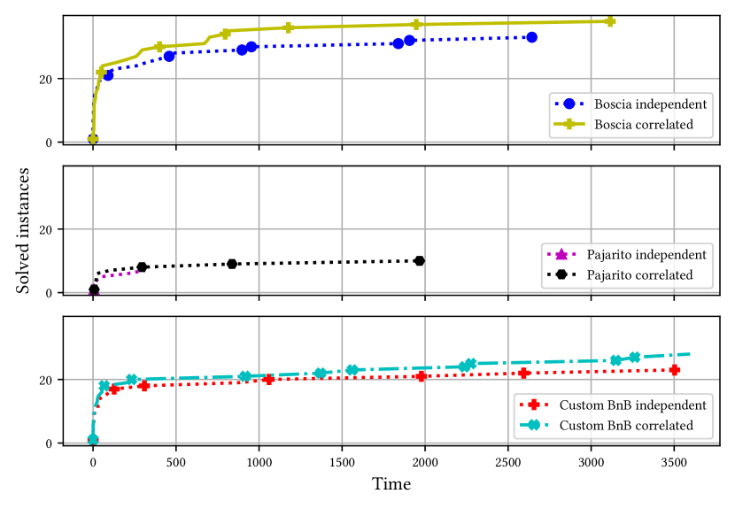
(a) A-Optimal Problem

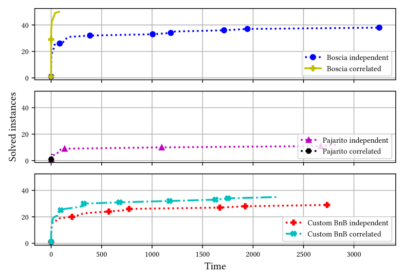
(b) D-Optimal Problem

Figure 1: The number of instances solved to optimality over time for the A-Optimal Problem and D-Optimal Problem with both data sets. The upper-most plot shows Boscia.jl, the middle Pajarito.jl  and the bottom Co-BnB.

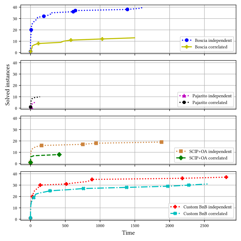
(a) A-Fusion Problem

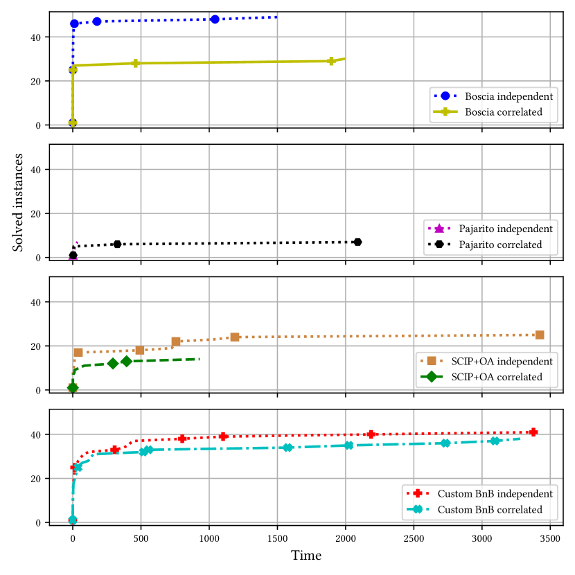
(b) D-Fusion Problem

Figure 2: The number of instances solved to optimality over time for the A-Fusion Problem and D-Fusion Problem with both data sets. The upper-most plot shows Boscia.jl, the upper-middle Pajarito.jl, and the bottom SCIP.

Notice that there is a sharp increase in the beginning, especially for Co-BnB and Boscia.jl. In contrast to Boscia.jl, the curves for Co-BnB flatten more after the first 10 seconds. The notable exception is the A-Fusion Problem with correlated data for which the Co-BnB method works consistently better than Boscia.jl, see also Table 1. As previously stated, the Co-BnB framework was developed for the case where the number of parameters $n$, and consequently the number of allowed experiment N, is significantly smaller than the number of experiments $m$. There are no advanced Branch-and-Bound tree specifications implemented like a better traverse strategy etc. A greater value of $N$ naturally increases the size of the tree and the number of nodes to be processed. Boscia.jl has the advantage here since it finds many integer feasible points while solving the relaxations which have the potential to improve the incumbent. A better incumbent, in turn, lets us prune non-improving nodes early on.

Observe that the curves for the two Outer Approximation approaches also flatten out. In addition, their increase at the start is not as sharp as for the two Branch-and-Bound approaches. Keep in mind that while the sub-problems, that is the relaxations, of the two Branch-and-Bound approaches, keep the simple feasible region intact, the Outer Approximation methods add many additional constraints, i.e. the cuts. This results in larger LPs to be solved. Furthermore, these cuts are dense leading to further difficulty for the LP solvers.

Aside from the performance comparison of the solvers, we investigate how the problems themselves compare to each other and if the difficulty of the instances is solver-dependent or if there are clear trends.

It can be observed in Table 1 that most solvers solve fewer instances under the A-criterion. The notable exception is Pajarito.jl on the A-Optimal Problem where it solves more instances to optimality compared to the D-criterion. It should be noted, however, that Pajarito.jl encountered slow progress for many instances under the A-criterion because too many cuts were added or the cuts were too close, i.e. the normal vectors of the hyperplane too parallel to each other.

Taking a look at some example contour plots shown in Figure 3, we observe that the contour lines for the A-criterion are steeper than those of the D-criterion for both the Optimal Problem and the Fusion Problem, respectively. This points to the conditioning increasing.

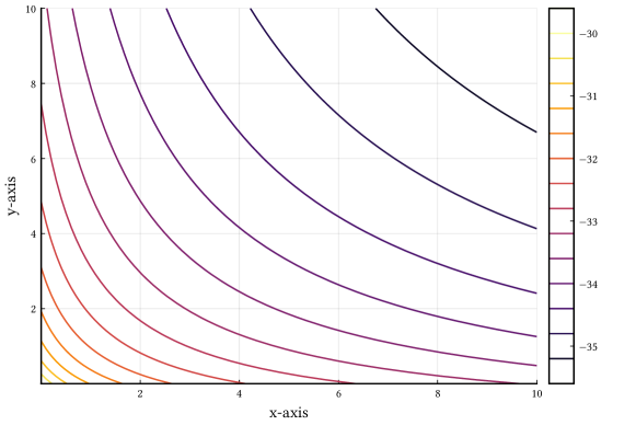
(a) D-Optimal Correlated

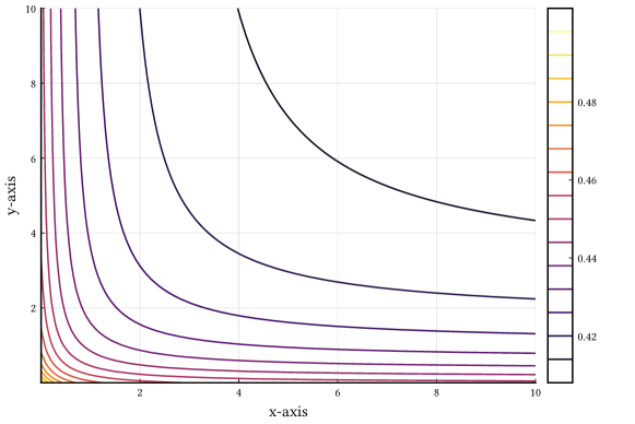
(b) A-Optimal Correlated

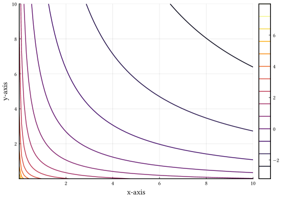
(c) D-Fusion Independent

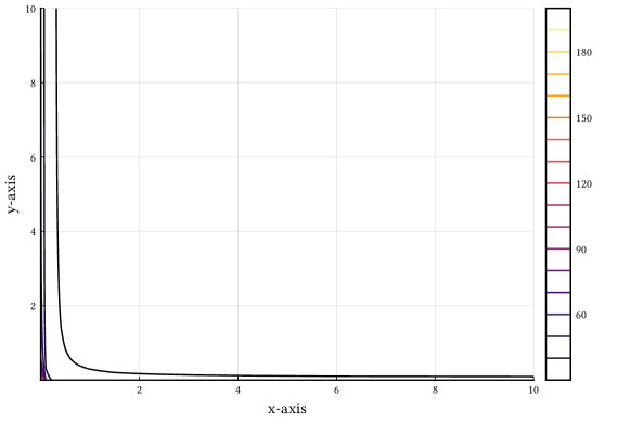
(d) A-Fusion Independent

Figure 3: Example contour plots in two dimensions for objectives of both Optimal Problems with correlated data and both Fusion Problems with independent.

In terms of the data, one could assume that all problems would be easier to solve with independent data. Noticeably, this is not the case. Rather, it differs for the two problem types. The Fusion Problems are easier with independent data, the Optimal Problems are more often solved with the correlated data. Figures 4(a) to 4(d) depict the progress of the incumbent, lower bound, and dual gap within Boscia.jl for selected instances of each combination of problem and data type.

Interestingly, the independent data leads to proof of optimality, i.e. the optimal solution is found early on and the lower bound has to close the gap, regardless of the problem, see Figures 4(a) and 4(c). The difference in problems has, however, an impact on how fast the lower bound can catch up with the incumbent. Comparing Figures 4(a) and 4(c), the lower bound curve in Figure 4(c) gets closer to the incumbent initially, i.e. in the first 2 seconds, and flattens more compared to the lower bound curve in Figure 4(a). The reason for this difference is likely that in the case of the Optimal Problem there is a larger region around the optimal solution where the corresponding points/designs $\mathbf{x}$ provide roughly the same information. These other candidates have to be checked to ensure the optimality of the incumbent and thus the solving process slows down. If we can prove either strong convexity or sharpness for the objectives, this xan potentially be used to speed up the progress of the lower bound. Currently, Boscia.jl can only utilize strong convexity but the adaptation for sharpness is in development.

On the other hand, the correlated data leads to solution processes that are very incumbent-driven, i.e. most improvement on the dual gap stems from the improving incumbent, not from the lower bound, as seen in Figures 4(b) and 4(d). Incumbent-driven solution processes can be identified by the dual gap making sudden jumps and the absence of (a lot of) progress between these jumps. As before, the solution process speed depends on the Problem. In Figure 4(b), the dual gap makes big jumps throughout most of the solving process, in contrast to the dual gap Figure 4(d). This indicates that the optimal solution of the Fusion Problem is strictly in the interior and thus, will not be found early as a vertex of a relaxation. The key ingredient for improvement in this case will be the incorporation of more sophisticated primal heuristics in Boscia.jl.

(a) $m=60$ and $n=15$

(b) $m=100$ and $n=10$

(c) $m=100$ and $n=10$

(d) $m=80$ and $n=20$

Figure 4: Progress of the incumbent and the lower bound on the left and progress of the dual gap for (a) the A-Optimal Problem with independent data, (b) the D-Optimal with correlated data and the A-Fusion Problem with (c) independent and (d) correlated data.

Table 1: Comparing Boscia, Pajarito, SCIP and Co-BnB on the different problems and the different data sets, i.e. A-Fusion (AF), D-Fusion (DF), A-Optimal (AO) and D-Optimal (DO). One data set contains independent data, the other has correlated data.
The instances for each problem are split into increasingly smaller subsets depending on their minimum solve time, i.e. the minimum time any of the solvers took to solve it. The cut-offs are at 0 seconds (all problems), took at least 10 seconds to solve, 100 s, 1000 s and lastly 2000 s. Note that if none of the solvers terminates on any instance of a subset, the corresponding row is omitted from the table.
The average time is taken using the geometric mean shifted by 1 second. Also note that this is the average time over all instances in that group, i.e. it includes the time outs.

				Boscia			Pajarito			SCIP			Co-BnB
Type	Corr.	Solved after (s)	# inst.		% solved	Time (s)		% solved	Time (s)		% solved	Time (s)		% solved	Time (s)
AF	no	0	50		80 %	52.51		12 %	2006.81		38%	453.68		74 %	90.33
		10	30		67 %	376.42		0 %	3600.03		7 %	3080.35		57 %	672.35
		100	20		50 %	1311.86		0 %	3600.04		%0	3600.04		35 %	2153.83
		1000	13		23 %	2954.49		0 %	3600.051		0 %	3600.032		8 %	3464.658
AF	yes	0	50		26 %	1330.74		20 %	1132.66		16 %	1350.87		62 %	170.03
		10	37		14 %	2583.78		0%	3600.06		3 %	3395.67		49 %	764.93
		100	28		11 %	2969.69		0 %	3600.06		0 %	3600.10		32 %	2141.55
		1000	22		0 %	3600.10		0 %	3600.06		0 %	3600.08		14 %	3322.80
		2000	21		0 %	3600.11		0 %	3600.07		0 %	3600.09		10 %	3464.44
AO	no	0	50		66 %	155.16		14 %	1901.70		-	-		46 %	440.57
		10	36		53 %	763.61		0 %	3600.06		-	-		25 %	2256.08
		100	28		39 %	1825.55		0 %	3600.061		-	-		7 %	3406.153
		1000	20		15 %	3321.23		0 %	3600.08		-	-		0 %	3600.069
		2000	18		6 %	3539.68		0 %	3600.089		-	-		0 %	3600.074
AO	yes	0	50		76 %	139.21		20 %	1591.74		-	-		56 %	323.80
		10	32		62 %	627.59		0 %	3600.051		-	-		34 %	1786.85
		100	26		54 %	1330.82		0 %	3600.06		-	-		19 %	3218.75
		1000	14		14 %	3181.23		0 %	3600.10		-	-		14 %	3455.49
		2000	12		0 %	3600.47		0 %	3600.08		-	-		8 %	3460.17
DF	no	0	50		98 %	2.35		14 %	1576.50		50 %	299.62		82 %	43.06
		10	5		80 %	419.46		0 %	3613.30		0 %	3600.08		0 %	3600.53
		100	4		75 %	1000.68		0 %	3612.67		0 %	3600.10		0 %	3600.57
		1000	3		67 %	1779.29		0 %	3613.69		0 %	3600.10		0 %	3600.75
DF	yes	0	50		60 %	48.48		14 %	1761.18		28 %	765.33		76 %	71.16
		10	20		15 %	2363.74		0 %	3607.12		0 %	3600.06		40 %	1192.27
		100	17		12 %	3080.74		0 %	3606.75		0 %	3600.06		29 %	2234.45
		1000	13		8 %	3439.43		0 %	3608.44		0 %	3600.06		8 %	3574.11
DO	no	0	50		76 %	70.87		24 %	1484.13		-	-		58 %	221.06
		10	30		60 %	641.92		3 %	3567.48		-	-		30 %	2250.58
		100	24		50 %	1360.11		4 &	3559.30		-	-		12 %	3358.04
		1000	18		33 %	2735.60		0 %	3605.13		-	-		0 %	3600.04
		2000	13		8 %	3572.83		0 %	3600.20		-	-		0 %	3600.05
DO	yes	0	50		100 %	1.33		10 %	1815.75		-	-		70 %	115.42
		10	7		100 %	29.79		0 %	3609.42		-	-		0 %	3600.04

6 Conclusion

We proposed a new approach for the Optimal Experiment Design Problem based on the Boscia framework, and show its performance compared to other MINLP approaches. In addition, it also performs better compared to the approach specifically developed for the OEDP, in particular for large-scale instances and a larger number of parameters. This superiority can be explained by the fact that Boscia.jl keeps the structure of the problem and that it utilizes a combinatorial solver to find integer feasible points at each node.

6.0.1 Acknowledgements

Research reported in this paper was partially supported through the Research Campus Modal funded by the German Federal Ministry of Education and Research (fund numbers 05M14ZAM,05M20ZBM) and the Deutsche Forschungsgemeinschaft (DFG) through the DFG Cluster of Excellence MATH+.

Appendix 0.A Convergence proofs on continuous relaxations

0.A.1 Lipschitz smoothness of the Fusion Problems

The convergence analysis for Frank-Wolfe algorithms relies on the fact that the objective function values do not grow arbitrarily large. The property guaranteeing this is Lipschitz smoothness, further called $L$-smoothness.

Definition 5

A function $f:{\mathbb{R}}^{n}\rightarrow{\mathbb{R}}$ is called $L$-smooth if its gradient $\nabla f$ is Lipschitz continuous. That is, there exists a finite $L\in{\mathbb{R}}$ with

$$\left\|\nabla f(\mathbf{x})-\nabla f(\mathbf{y})\right\|_{2}\leq L\left\|\mathbf{x}-\mathbf{y}\right\|_{2}.$$

Since the functions of interest are in $\mathcal{C}^{3}$, we can use an alternative condition on $L$-smoothness: $LI\succcurlyeq\nabla_{xx}f(\mathbf{x})$, i.e. the Lipschitz constant $L$ is at least as large as the maximum eigenvalue of the Hessian.

We will see that we have $L$-smoothness on the whole convex feasible region $\mathcal{P}$ only for the Fusion Problems. Due to the positive definiteness of the matrix $C$, the information matrix in the Fusion case $X_{C}(\mathbf{x})$ is always bounded away from the boundary of the PSD cone. As for the Optimal Problems, we will prove self-concordance in Section 0.A.2 to consequently show convergence for Frank-Wolfe.

Before we investigate $L$-smoothness, we first prove a relationship between a matrix $X$ and its power matrix $X^{r}$ where $r\in{\mathbb{R}}\backslash\{0\}$.

Lemma 1

Let $X\in{\mathbb{R}}^{n\times n}$ by an invertible matrix and $r\in{\mathbb{R}}\backslash\{0\}$. Then, the eigenvalues of the power matrix are:

$$\lambda_{i}(X^{r})=\lambda_{i}(X)^{r}\quad\forall i=[n]$$

and the eigenvectors of the power matrix are the same as those of $X$.

Proof

Let $\mathbf{v}$ be an eigenvector of $X$ and let $\lambda_{\mathbf{v}}$ denote the corresponding eigenvalue.

$$X^{r}\mathbf{v} =\left(\sum\limits_{k=0}^{\infty}\frac{r^{k}}{k!}\log(X)^{k}\right)\mathbf{v}=\sum\limits_{k=0}^{\infty}\frac{r^{k}}{k!}\log(X)^{k}\mathbf{v}$$

For any square matrix $$A m A^{m}\mathbf{v}=\lambda_{\mathbf{v}}(A)^{m}\mathbf{v} A \log(\lambda_{i}(A))$$ and a positive integer , we have that . Also, the logarithm of a matrix has the same eigenvectors as the original and its eigenvalues are .

$$=\left(\sum\limits_{k=0}^{\infty}\frac{r^{k}\log(\lambda_{\mathbf{v}}(X))^{k}}{k!}\right)\mathbf{v}=\exp(r\log(\lambda_{\mathbf{v}}(X)))\mathbf{v}$$

$$=\lambda_{\mathbf{v}}(X)^{r}\mathbf{v}$$

This concludes the proof. ∎

Corollary 1

For $r\in{\mathbb{R}}\backslash\{0\}$, if $X\in\mathbb{S}_{++}^{n}$, then $X^{r}\in\mathbb{S}_{++}^{n}$.

Let us now prove $L$-smoothness for the Fusion Problems under the A-criterion and D-criterion.

Theorem 0.A.1

The functions $f_{F}(\mathbf{x}):=-\log\det\left(X_{C}(\mathbf{x})\right)$ and $g_{F}(\mathbf{x}):=\operatorname{Tr}\left(\left(X_{C}(\mathbf{x})\right)^{-p}\right)$ for $p\in{\mathbb{R}}_{>0}$ are $L$-smooth with Lipschitz constants

$$L_{f}=\left(\max\limits_{i}(AA^{\intercal})_{ii}\right)\frac{\|A\|_{2}^{2}}{\lambda_{\min}(C)^{2}}$$

and

$$L_{g}=p(p+1)\left(\max\limits_{i}(AA^{\intercal})_{ii}\right)\frac{\left\|A\right\|_{2}^{2}}{\lambda_{\min}(C)^{2+p}},$$

respectively.

Proof

For better readability and simplicity, we ignore the dependency on $\mathbf{x}$ for now. As stated above, we can prove $L$-smoothness by showing that the largest eigenvalue of the Hessians is bounded for any $\mathbf{x}$ in the domain. We have

$$\nabla^{2}f(\mathbf{x}) =(AA^{\intercal})\circ(AX_{C}^{-2}A^{\intercal})$$

and

$$\nabla^{2}g(\mathbf{x}) =p(p+1)\left(AA^{\intercal}\right)\circ\left(AX_{C}^{-p-2}A^{\intercal}\right).$$

Observe that the Hessian expressions are very similar. Hence, we will only present the proof for $$g f N M \lambda_{\max}(N\circ M) N M$$. The proof of follows the same argumentation. By (Horn, 1990, page 95) it is known that the maximum eigenvalue of a Hadamard product between two positive semi-definite matrices and , , is upper-bounded by the maximum diagonal entry of and the largest eigenvalue of , so

$$\lambda_{\max}(N\circ M) \leq\max_{i}N_{ii}\lambda_{\max}(M).$$ (3)

In our case, $$N=AA^{\intercal} M=AX_{C}^{-p-2}A^{\intercal} X_{C}^{-p-2}$$ and . By Corollary 1 we have that is positive definite. Thus, both factors are semi-definite and thus we may use the provided bound:

$$\lambda_{\max}\left(\nabla^{2}g(\mathbf{x})\right) \leq\max\limits_{i}(AA^{\intercal})_{ii}\lambda_{\max}(AX_{C}^{-p-2}A^{\intercal}).$$

Note that the first factor is simply:

$$\max\limits_{i}(AA^{\intercal})_{ii} =\max\limits_{i}\mathbf{v}_{i}^{\intercal}\mathbf{v}_{i}.$$ (4)

For the second factor, we can exploit positive semi-definiteness with the spectral norm:

$$\lambda_{\max}\left(AX_{C}^{-p-2}A^{\intercal}\right) =\left\|AX_{C}^{-p-2}A^{\intercal}\right\|_{2}$$

$$\leq\left\|A\right\|_{2}^{2}\left\|X_{C}^{-p-2}\right\|_{2}.$$

By Lemma 1, we have:

$$\lambda(A^{p}) =\lambda(A)^{p}$$

$$=\left\|A\right\|_{2}^{2}\lambda_{\max}(X_{C}^{-1})^{2+p}$$

$$=\frac{\left\|A\right\|_{2}^{2}}{\lambda_{\min}(X_{C})^{2+p}}.$$

By the definition of $$X$$ and by Weyl’s inequality on the eigenvalues of sums of positive semi-definite matrices (Weyl, 1912), we have that:

$$\lambda_{\min}(X_{C}) \geq\lambda_{\min}(C)+\lambda_{\min}(A^{\intercal}\operatorname{diag}(x)A)\geq\lambda_{\min}(C).$$

Hence,

$$\lambda_{\max}\left(AX_{C}^{-p-2}A^{\intercal}\right) \leq\frac{\left\|A\right\|_{2}^{2}}{\lambda_{\min}(C)^{2+p}}.$$ (5)

Combining (3) with (4) and (5) yields

$$\lambda_{\max}\left(\nabla^{2}g(\mathbf{x})\right) \leq p(p+1)\left(\max\limits_{i}v_{i}^{\intercal}v_{i}\right)\frac{\left\|A\right\|_{2}^{2}}{\lambda_{\min}(C)^{2+p}}.$$ (6)

This concludes the proof. ∎

Note that the proof works because we can bound the minimum eigenvalue of $X_{C}$ away from zero thanks to the positive definite matrix $C$. This is not the case for the information matrices $X(\mathbf{x})$ of the Optimal Problems as they can be singular.

0.A.2 Generalized Self-Concordance

Lacking $L$-smoothness on the feasible region for the Optimal Problems, we need a different property guaranteeing convergence. As stated in Section 3, we can prove that the objective function resulting from the A-criterion is generalized self-concordant to establish convergence of Frank-Wolfe. In fact, we can prove the statement for the General-Trace-Inverse (GTI) $g(x)=\operatorname{Tr}\left(X^{-p}\right)$ for $p>0$.

First, we need to compute the first three partial derivatives of $g$. To help us in this endeavor, we prove the following lemma.

Lemma 2

Let $r\in{\mathbb{R}}$ and let the matrix $X$ be diagonalizable. Then, we can define the function $f(X)=\operatorname{Tr}(X^{r})$. The gradient of $f$ is then

$$\nabla f(x)=rX^{r-1}$$

Proof

We use the definition of $X^{r}$ to prove the result.

$$\operatorname{Tr}(X^{r}) =\operatorname{Tr}\left(\sum\limits_{k=0}^{\infty}\frac{r^{k}}{k!}\log(X)^{k}\right)=\sum\limits_{k=0}^{\infty}\frac{r^{k}}{k!}\operatorname{Tr}\left(\log(X)^{k}\right)$$

Thus, using the sum rule, $$(\operatorname{Tr}(X^{n}))^{\prime}=nX^{n-1} n \nabla\operatorname{Tr}(\log(X))=X^{-1}$$ for any positive integer and , we have

$$\nabla\operatorname{Tr}(X^{r}) =\sum\limits_{k=1}^{\infty}\frac{r^{k}}{k!}k{\log(X)}^{k-1}X^{-1}$$

$$=rX^{-1}\sum\limits_{k=0}^{\infty}\frac{r^{k}}{k!}\log(X)^{k}$$

$$=rX^{-1}X^{r}=rX^{r-1}$$

This concludes the proof. ∎

Let $A\in\mathbb{S}_{++}^{n},B\in\mathbb{S}_{+}^{n}$ and $t\in{\mathbb{R}}$ such that $A+tB\in\mathbb{S}_{++}^{n}$. We define $h(t)=g(A+tB)$. For the proof of self-concordance, we need the first three derivatives of $h(t)$.

$$h(t) =\operatorname{Tr}((A+tB)^{-p})=\operatorname{Tr}\left(\left((A+tB)^{-1}\right)^{p}\right)$$

Using Lemma 2 for the first derivative, yields:

$$h^{\prime}(t) =\operatorname{Tr}\left(p\left((A+tB)^{-1}\right)^{p-1}(-1)(A+tB)^{-1}B(A+tB)^{-1}\right)$$

$$=-p\operatorname{Tr}\left(\left((A+tB)^{-1}\right)^{p}B(A+tB)^{-1}\right).$$

For the second derivative, we find

$$h^{\prime\prime}(t) =-p\operatorname{Tr}\left(p\left((A+tB)^{-1}\right)^{p-1}(-1)(A+tB)^{-1}B(A+tB)^{-1}B(A+tB)^{-1}\right.$$

$$\left.\quad+\left((A+tB)^{-1}\right)^{p}B(-1)(A+tB)^{-1}B(A+tB)^{-1}\vphantom{\left((A+tB)^{-1}\right)^{p-1}}\right)$$

$$=p\operatorname{Tr}\left((p+1)\left((A+tB)^{-1}\right)^{p}B(A+tB)^{-1}B(A+tB)^{-1}\right).$$

Restricting $$h^{\prime\prime} t=0$$ to , yields:

$$h^{\prime\prime}(t)_{\restriction t=0} =p(p+1)\operatorname{Tr}\left(A^{-p}BA^{-1}BA^{-1}\right).$$

Lastly, for the third derivative, we have:

$$h^{\prime\prime\prime}(t) =p(p+1)\operatorname{Tr}\left(p\left((A+tB)^{-1}\right)^{p-1}(-1)(A+tB)^{-1}B(A+tB)^{-1}B(A+tB)^{-1}B(A+tB)^{-1}\right.$$

$$\left.\quad+2\left((A+tB)^{-1}\right)^{p}(-1)B(A+tB)^{-1}B(A+tB)^{-1}B(A+tB)^{-1}\vphantom{\left((A+tB)^{-1}\right)^{p-1}}\right).$$

And restricted to $$t=0$$, yields:

$$h^{\prime\prime\prime}(t) =-p(p+1)(p+2)\operatorname{Tr}\left((A+tB)^{-p}B(A+tB)^{-1}B(A+tB)^{-1}B(A+tB)^{-1}\right).$$

In the following theorem, we show that $g(X)=\operatorname{Tr}\left(X^{-p}\right)$ with $p>0$ is self-concordant on a part of the PSD cone, characterized by an upper bound on the maximum eigenvalue.

Theorem 0.A.2

The function $g(X)=\operatorname{Tr}\left(X^{-p}\right)$, with $p>0$, is $\left(3,\frac{(p+2)\sqrt[4]{a^{2p}n}}{\sqrt{p(p+1)}}\right)$-generalized self-concordant on $\mathrm{dom}(f)=\left\{X\in\mathbb{S}_{++}^{n}\mid 0\prec X\preccurlyeq aI\right\}$ where $a\in{\mathbb{R}}_{>0}$ bounds the maximum eigenvalue of $X$.

Proof

We define $M(t)=V+tU$ where $V\in\mathrm{dom}(g)$, $U\in\mathbb{S}_{+}^{n}$ and $t\in{\mathbb{R}}$ such that $V+tU\in\mathbb{S}_{++}^{n}$. Then:

$$h(t) =g(M(t))=\operatorname{Tr}\left(M(t)^{-p}\right).$$

From the derivative computation above, we have

$$h^{\prime\prime}(t)_{\restriction t=0} =p(p+1)\operatorname{Tr}\left(V^{-p}UV^{-1}UV^{-1}\right)$$

$$h^{\prime\prime\prime}(t)_{\restriction t=0} =-p(p+1)(p+2)\operatorname{Tr}\left(V^{-p}UV^{-1}UV^{-1}UV^{-1}\right).$$

Thus, the condition we want to satisfy is:

$$p(p+1)(p+2)\operatorname{Tr}\left(V^{-p}UV^{-1}UV^{-1}UV^{-1}\right) \leq M_{f}p(p+1)Tr\left(V^{-p}UV^{-1}UV^{-1}\right)^{\nu-2}.$$

Note that

$$\operatorname{Tr}\left(V^{-p}UV^{-1}UV^{-1}UV^{-1}\right)=\operatorname{Tr}\left(V^{-\frac{p+1}{2}}UV^{-1}UV^{-1}UV^{-\frac{p+1}{2}}\right)\geq 0$$

and

$$\operatorname{Tr}\left(V^{-p}UV^{-1}UV^{-1}\right)=\operatorname{Tr}\left(V^{-\frac{p+1}{2}}UV^{-1}UV^{-\frac{p+1}{2}}\right)\geq 0$$

by positive definiteness of $V$ and semi-definiteness $U$. If the trace is equal to 0, the statement holds directly. Otherwise, we divide both sides by the LHS and first try to lower bound the following fraction:

$$\frac{\operatorname{Tr}\left(V^{-\frac{p+1}{2}}UV^{-1}UV^{-\frac{p+1}{2}}\right)^{\nu-2}}{\operatorname{Tr}\left(V^{-\frac{p+1}{2}}UV^{-1}UV^{-1}UV^{-\frac{p+1}{2}}\right)}.$$

We want to lower-bound this fraction. To that end, we define $H=V^{-1/2}UV^{-1/2}$ and $L=V^{-p/2}H$, then:

$$\frac{\operatorname{Tr}\left(V^{-\frac{p+1}{2}}UV^{-1}UV^{-\frac{p+1}{2}}\right)^{\nu-2}}{\operatorname{Tr}\left(V^{-\frac{p+1}{2}}UV^{-1}UV^{-1}UV^{-\frac{p+1}{2}}\right)} =\frac{\operatorname{Tr}\left(LL^{\intercal}\right)^{\nu/2}}{\operatorname{Tr}\left(LHL^{\intercal}\right)}.$$

Using Cauchy-Schwartz, we find:

$$\operatorname{Tr}\left(LHL^{\intercal}\right) =\left\langle L^{\intercal}L,H\right\rangle$$

$$\leq\operatorname{Tr}\left(LL^{\intercal}\right)\sqrt{\operatorname{Tr}\left(H^{2}\right)}$$

$$\frac{\operatorname{Tr}\left(LL^{\intercal}\right)^{\nu/2}}{\operatorname{Tr}\left(LHL^{\intercal}\right)} \geq\frac{\operatorname{Tr}\left(LL^{\intercal}\right)^{\nu/2}}{\operatorname{Tr}\left(LL^{\intercal}\right)\sqrt{\operatorname{Tr}\left(H^{2}\right)}}$$

$$\operatorname{Tr}\left(HH\right) =\operatorname{Tr}\left(V^{p/2}V^{-p/2}HHV^{-p/2}V^{p/2}\right)$$

$$=\operatorname{Tr}\left(V^{p/2}LL^{\intercal}V^{p/2}\right)$$

$$\leq\operatorname{Tr}\left(LL^{\intercal}\right)\sqrt{\operatorname{Tr}\left(V^{2p}\right)}$$

$$\frac{\operatorname{Tr}\left(LL^{\intercal}\right)^{\nu/2}}{\operatorname{Tr}\left(LL^{\intercal}\right)\sqrt{\operatorname{Tr}\left(H^{2}\right)}} \geq\frac{\operatorname{Tr}\left(LL^{\intercal}\right)^{\nu/2}}{\operatorname{Tr}\left(LL^{\intercal}\right)\sqrt{\operatorname{Tr}\left(LL^{\intercal}\right)\sqrt{\operatorname{Tr}\left(V^{2p}\right)}}}$$

$$=\operatorname{Tr}\left(LL^{\intercal}\right)^{\nu/2-3/2}\frac{1}{\sqrt{\left\|V^{p}\right\|_{F}}}$$

$$\geq\operatorname{Tr}\left(LL^{\intercal}\right)^{\nu/2-3/2}\frac{1}{\sqrt{\left\|V^{p}\right\|_{2}}\sqrt[4]{n}}.$$

By the assumption that V is a feasible point, we have $$\left\|V\right\|_{2}=\lambda_{\max}(V)\leq a$$, thus:

$$\frac{\operatorname{Tr}\left(LL^{\intercal}\right)^{\nu/2}}{\operatorname{Tr}\left(LL^{\intercal}\right)\sqrt{\operatorname{Tr}\left(H^{2}\right)}} \geq\operatorname{Tr}\left(LL^{\intercal}\right)^{\nu/2-3/2}\frac{1}{\sqrt{a^{p}}\sqrt[4]{n}}.$$

Then,

$$\frac{M_{f}(p(p+1))^{\nu/2}}{p(p+1)(p+2)}\frac{\operatorname{Tr}\left(V^{-p}UV^{-1}UV^{-1}\right)^{\nu-2}}{\operatorname{Tr}\left(V^{-p}UV^{-1}UV^{-1}UV^{-1}\right)} \geq\frac{M_{f}(p(p+1))^{\nu/2}}{p(p+1)(p+2)}\operatorname{Tr}\left(LL^{\intercal}\right)^{\nu/2-3/2}\frac{1}{\sqrt{a^{p}}\sqrt[4]{n}}.$$

We can select $$\nu=3$$ and re-express the GSC condition as

$$1 \leq\frac{M_{f}(p(p+1))^{1/2}}{(p+2)}\frac{1}{\sqrt[4]{a^{2p}n}}.$$

$$M_{f} \geq\frac{(p+2)\sqrt[4]{a^{2p}n}}{\sqrt{p(p+1)}}.$$

Thus, $g$ is $\left(3,\frac{(p+2)\sqrt[4]{a^{2p}n}}{\sqrt{p(p+1)}}\right)$-generalized self-concordant. ∎

Corollary 2

The function $g(X)=\operatorname{Tr}\left(X^{-1}\right)$ is $\left(3,\frac{3\sqrt[4]{a^{2}n}}{\sqrt{2}}\right)$-generalized self-concordant on $\mathrm{dom}(g)=\left\{X\mid 0\prec X\preccurlyeq aI\right\}$.

To ensure that Theorem 0.A.2 is applicable for the objective of the (A-Opt), we show that the maximum eigenvalue of the information matrix is bounded.

Lemma 3

Let $x\in\mathcal{P}$. Then,

$$\lambda_{\max}(X(\mathbf{x}))\leq\max_{i}u_{i}\max_{i}\left\|\mathbf{v}_{i}\right\|_{2}^{2}.$$

where $\mathbf{u}$ denotes the upper bounds and $\mathbf{v}_{i}$ are the rows of the experiment matrix $A$.

Proof

$$\lambda_{\max}(X(\mathbf{x})) =\lambda_{\max}\left(\sum\limits_{i=1}^{m}x_{i}\mathbf{v}_{i}\mathbf{v}_{i}^{\intercal}\right).$$

By the Courant Fischer Min-Max Theorem, we have:

$$\lambda_{\max}(X(\mathbf{x})) \leq\sum\limits_{i=1}^{m}\lambda_{\max}\left(x_{i}\mathbf{v}_{i}\mathbf{v}_{i}^{\intercal}\right).$$

Using $$\mathbf{x}\leq\mathbf{u}$$, yields:

$$\lambda_{\max}(X(\mathbf{x})) \leq\max_{i}u_{i}\max_{i}\left\|\mathbf{v}_{i}\right\|_{2}^{2}.$$

∎

Combing Theorem 0.A.2 and Lemma 3, yields:

Corollary 3

The function $g(\mathbf{x})=\operatorname{Tr}\left(X(\mathbf{x})^{-p}\right)$ is self-concordant on the convex feasible region $\mathcal{P}$.

Appendix 0.B Notes on Custom Branch-and-Bound Algorithm for the Exact Optimal Design Problem

In this section, we showcase the changes we made to the solver set-up in Ahipaşaoğlu (2021). Firstly, we state and solve the problems of interest as minimization problems. Secondly, we forgo the $\mathbf{w}N\in{\mathbb{Z}}\,\forall i\in[m]$ in favor of directly having the variables $x$ to encode if and how often the experiments should be run. The D-Optimal Problem is then stated as

$$\min_{\mathbf{x}}\, \,-\log\det\left((X(\mathbf{x}))\right)$$

s.t. $$\sum\limits_{i=1}^{m}x_{i}=N$$

$$\mathbf{x}\geq 0$$

$$x_{i}\in{\mathbb{Z}}\,\forall i\in[m].$$

The A-Optimal Problem is formulated as

$$\min_{\mathbf{x}}\, \,\log\left(\operatorname{Tr}(X^{-1})\right)$$

s.t. $$\sum\limits_{i=1}^{m}x_{i}=N$$

$$\mathbf{x}\geq 0$$

$$x_{i}\in{\mathbb{Z}}\,\forall i\in[m].$$

Additionally, we have adapted the step size for the A-Optimal Problem. For the update in the objective, we get

$$-\log(\operatorname{Tr}(X(\mathbf{x}_{+}))) =-\log(\operatorname{Tr}(X(\mathbf{x})^{-1})-\frac{\theta A+\theta^{2}B}{1+\theta C-\theta^{2}D})$$

compare Ahipaşaoğlu (2021, Section 4.2). The constant $$A B C D$$, , and are defined as

$$A =\zeta_{j}-\zeta_{k}$$

$$B =2\omega_{jk}\zeta_{jk}-\omega_{j}\zeta_{k}-\omega_{k}\zeta_{j}$$

$$C =\omega_{j}-\omega_{k}$$

$$D =\omega_{j}\omega_{k}-\omega_{jk}^{2}$$

where $$\omega_{j}=\mathbf{v}_{j}^{\intercal}X(x)^{-1}\mathbf{v}_{j} \zeta_{j}=\mathbf{v}_{j}^{\intercal}X(x)^{-2}\mathbf{v}_{j} \omega_{jk}=\mathbf{v}_{j}^{\intercal}X(x)^{-1}\mathbf{v}_{k} \zeta_{jk}=\mathbf{v}_{j}^{\intercal}X^{-2}\mathbf{v}_{k}$$ and , and and . The objective value should be improving.

$$-\log\operatorname{Tr}(X(\mathbf{x})^{-1}) \geq-\log\operatorname{Tr}(X(\mathbf{x}_{+})^{-1})$$

$$\operatorname{Tr}(X(\mathbf{x})^{-1}) \leq\operatorname{Tr}(X(\mathbf{x}_{+})^{-1})$$

$$=\operatorname{Tr}(X(\mathbf{x})^{-1})-\frac{\theta A+\theta^{2}B}{1+\theta C-\theta^{2}D}$$

Hence, we want to maximise the function $$q(\theta)=\frac{\theta A+\theta^{2}B}{1+\theta C-\theta^{2}D} \Delta=AD+BC$$. Let . By computing the first and second derivatives, it is easy to verify that we have

$$\theta^{*} =-\frac{B+\sqrt{B^{2}-A\Delta}}{\Delta}$$

if $$\Delta\neq 0 \Delta=0 B$$. If but is not, then we have

$$\theta^{*} =-\frac{A}{2B}.$$

If both $$B \Delta \theta$$ and are zero, then we choose as big as possible given the bound constraints.

$$\theta =\begin{cases}\min\left\{-\frac{B+\sqrt{B^{2}-A\Delta}}{\Delta},u_{j}-x_{j},x_{k}-l_{k}\right\}&\text{if }\Delta\neq 0\\ \min\left\{-\frac{A}{2B},u_{j}-x_{j},x_{k}-l_{k}\right\}&\text{if }\Delta=0\text{ and }B\neq 0\\ \min\{u_{j}-x_{j},x_{k}-l_{k}\}&\text{if }\Delta=B=0\text{ and }A>0\end{cases}$$

References

- Ahipaşaoğlu (2015) Ahipaşaoğlu, S. D. A first-order algorithm for the A-optimal experimental design problem: a mathematical programming approach. Statistics and Computing, 25(6):1113–1127, 2015.
- Ahipaşaoğlu (2021) Ahipaşaoğlu, S. D. A branch-and-bound algorithm for the exact optimal experimental design problem. Statistics and Computing, 31(5):65, 2021.
- Besançon et al. (2022) Besançon, M., Carderera, A., and Pokutta, S. FrankWolfe.jl: A high-performance and flexible toolbox for Frank–Wolfe algorithms and conditional gradients. INFORMS Journal on Computing, 2022.
- Bestuzheva et al. (2021) Bestuzheva, K., Besançon, M., Chen, W.-K., Chmiela, A., Donkiewicz, T., van Doornmalen, J., Eifler, L., Gaul, O., Gamrath, G., Gleixner, A., Gottwald, L., Graczyk, C., Halbig, K., Hoen, A., Hojny, C., van der Hulst, R., Koch, T., Lübbecke, M., Maher, S. J., Matter, F., Mühmer, E., Müller, B., Pfetsch, M. E., Rehfeldt, D., Schlein, S., Schlösser, F., Serrano, F., Shinano, Y., Sofranac, B., Turner, M., Vigerske, S., Wegscheider, F., Wellner, P., Weninger, D., and Witzig, J. The SCIP Optimization Suite 8.0, 2021.
- Bestuzheva et al. (2023) Bestuzheva, K., Besançon, M., Chen, W.-K., Chmiela, A., Donkiewicz, T., van Doornmalen, J., Eifler, L., Gaul, O., Gamrath, G., Gleixner, A., et al. Enabling research through the SCIP Optimization Suite 8.0. ACM Transactions on Mathematical Software, 49(2):1–21, 2023.
- Braun et al. (2017) Braun, G., Pokutta, S., and Zink, D. Lazifying conditional gradient algorithms. In International conference on machine learning, pp. 566–575. PMLR, 2017.
- Braun et al. (2022) Braun, G., Carderera, A., Combettes, C. W., Hassani, H., Karbasi, A., Mokhtari, A., and Pokutta, S. Conditional gradient methods. arXiv preprint arXiv:2211.14103, 2022.
- Carderera et al. (2021) Carderera, A., Besançon, M., and Pokutta, S. Simple steps are all you need: Frank–Wolfe and generalized self-concordant functions. Advances in Neural Information Processing Systems, 34:5390–5401, 2021.
- Coey et al. (2020) Coey, C., Lubin, M., and Vielma, J. P. Outer approximation with conic certificates for mixed-integer convex problems. Mathematical Programming Computation, 12(2):249–293, 2020.
- Coey et al. (2022a) Coey, C., Kapelevich, L., and Vielma, J. P. Conic optimization with spectral functions on Euclidean Jordan algebras. Mathematics of Operations Research, 2022a.
- Coey et al. (2022b) Coey, C., Kapelevich, L., and Vielma, J. P. Performance enhancements for a generic conic interior point algorithm. Mathematical Programming Computation, 2022b. doi: https://doi.org/10.1007/s12532-022-00226-0.
- Coey et al. (2022c) Coey, C., Kapelevich, L., and Vielma, J. P. Solving natural conic formulations with Hypatia.jl. INFORMS Journal on Computing, 34(5):2686–2699, 2022c. doi: https://doi.org/10.1287/ijoc.2022.1202.
- de Aguiar et al. (1995) de Aguiar, P. F., Bourguignon, B., Khots, M., Massart, D., and Phan-Than-Luu, R. D-optimal designs. Chemometrics and intelligent laboratory systems, 30(2):199–210, 1995.
- Frank & Wolfe (1956) Frank, M. and Wolfe, P. An algorithm for quadratic programming. Naval research logistics quarterly, 3(1-2):95–110, 1956.
- Hendrych et al. (2023) Hendrych, D., Troppens, H., Besançon, M., and Pokutta, S. Convex mixed-integer optimization with Frank–Wolfe methods, 2023.
- Horn (1990) Horn, R. A. The Hadamard product. In Proc. Symp. Appl. Math, volume 40, pp. 87–169, 1990.
- Huangfu & Hall (2018) Huangfu, Q. and Hall, J. J. Parallelizing the dual revised simplex method. Mathematical Programming Computation, 10(1):119–142, 2018.
- Kapelevich (2023) Kapelevich, L. How to optimize trace of matrix inverse with JuMP or Convex? https://discourse.julialang.org/t/how-to-optimize-trace-of-matrix-inverse-with-jump-or-convex/94167/6, accessed 4th December 2023, 2023.
- Kronqvist et al. (2019) Kronqvist, J., Bernal, D. E., Lundell, A., and Grossmann, I. E. A review and comparison of solvers for convex MINLP. Optimization and Engineering, 20:397–455, 2019.
- Levitin & Polyak (1966) Levitin, E. S. and Polyak, B. T. Constrained minimization methods. USSR Computational mathematics and mathematical physics, 6(5):1–50, 1966.
- Li et al. (2022) Li, Y., Fampa, M., Lee, J., Qiu, F., Xie, W., and Yao, R. D-optimal data fusion: Exact and approximation algorithms. arXiv preprint arXiv:2208.03589, 2022.
- Nesterov & Nemirovskii (1994) Nesterov, Y. and Nemirovskii, A. Interior-point polynomial algorithms in convex programming. SIAM, 1994.
- Nikolov et al. (2022) Nikolov, A., Singh, M., and Tantipongpipat, U. Proportional volume sampling and approximation algorithms for A-optimal design. Mathematics of Operations Research, 47(2):847–877, 2022.
- Ponte et al. (2023) Ponte, G., Fampa, M., and Lee, J. Branch-and-bound for D-optimality with fast local search and variable-bound tightening. arXiv preprint arXiv:2302.07386, 2023.
- Pukelsheim (2006) Pukelsheim, F. Optimal design of experiments. SIAM, 2006.
- Sagnol & Harman (2015) Sagnol, G. and Harman, R. Computing exact D-optimal designs by mixed integer second-order cone programming. 2015.
- Sahinidis & Grossmann (1991) Sahinidis, N. and Grossmann, I. E. Convergence properties of generalized benders decomposition. Computers & Chemical Engineering, 15(7):481–491, 1991.
- Sun & Tran-Dinh (2019) Sun, T. and Tran-Dinh, Q. Generalized self-concordant functions: a recipe for Newton-type methods. Mathematical Programming, 178(1-2):145–213, 2019.
- Welch (1982) Welch, W. J. Branch-and-bound search for experimental designs based on D optimality and other criteria. Technometrics, 24(1):41–48, 1982.
- Weyl (1912) Weyl, H. Das asymptotische Verteilungsgesetz der Eigenwerte linearer partieller Differentialgleichungen (mit einer Anwendung auf die Theorie der Hohlraumstrahlung). Mathematische Annalen, 71(4):441–479, 1912.