Learning from Imperfect Demonstrations through Dynamics Evaluation

Abstract

Standard imitation learning usually assumes that demonstrations are drawn from an optimal policy distribution. However, in real-world scenarios, every human demonstration may exhibit nearly random behavior and collecting high-quality human datasets can be quite costly. This requires imitation learning can learn from imperfect demonstrations to obtain robotic policies that align human intent. Prior work uses confidence scores to extract useful information from imperfect demonstrations, which relies on access to ground truth rewards or active human supervision. In this paper, we propose a dynamics-based method to evaluate the data confidence scores without above efforts. We develop a generalized confidence-based imitation learning framework called Confidence-based Inverse soft-Q Learning (CIQL), which can employ different optimal policy matching methods by simply changing object functions. Experimental results show that our confidence evaluation method can increase the success rate by $40.3\%$ over the original algorithm and $13.5\%$ over the simple noise filtering.

Index Terms— Imitation Learning, Manipulation Planning, Learning from Demonstration

I INTRODUCTION

Imitation learning (IL) attracts much attention for its potential to enable robots to complete complex tasks from human demonstrations. Traditional IL typically depends on large-scale, high-quality, and diverse human datasets to achieve satisfactory results[1, 2, 3]. In real-world scenarios, collecting such human datasets can be quite costly. When using specialized data collection system, human operators may provide noisy demonstrations due to factors such as fatigue, distraction, or lack of skill[4]. Each human demonstration has the potential to exhibit nearly random behavior. The well performing trajectories may still contain some noise, which can have a negative impact on the performance of standard IL[5]. The poorly performing or even unsuccessful trajectories may contain useful information. It is difficult for humans to provide perfect trajectories, and these imperfect demonstrations can not accurately reflect the expert’s true intent. In this paper, we aim to maximize the use of limited human imperfect demonstrations to learn policy that align human intent.

Learning from imperfect demonstrations is nothing new, and its work falls into two main directions: ranking-based and confidence-based. For the ranking-based approach, it learns a reward function that satisfies the ranking of trajectories through supervised learning, and then improves the policy through reinforcement learning[6, 7, 8]. This approach depends on the availability of high-quality datasets to learn a robust reward function. For the confidence-based approach, it uses confidence scores to describe the quality of demonstrations in order to extract useful information from imperfect demonstrations while filtering noise efficiently[9, 10, 11]. The key challenge with this approach is how to get the true data confidence scores.

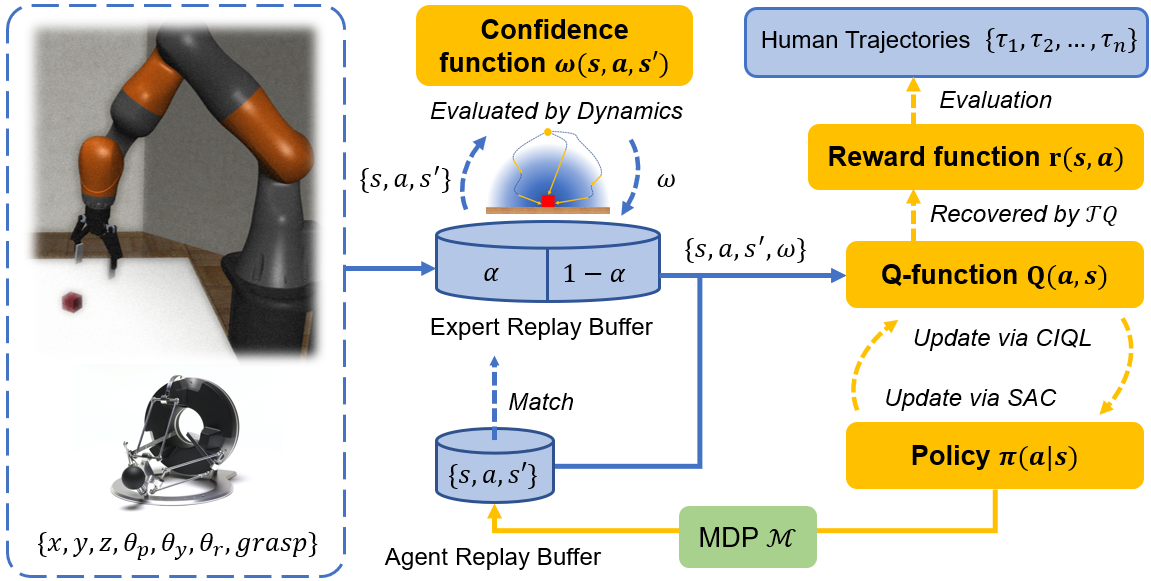
Figure 1: Overview of Confidence-based Inverse soft-Q Learning (CIQL): (1) Use the confidence function $w$ to label the transitions $\{s,a,s^{\prime}\}$ and estimate the optimal priori probability $\alpha$ (2) Sample a batch of transitions from the expert and agent replay buffers, learn the optimal Q-function via CIQL, and improve the policy via Soft Actor-Critic (SAC). (3) Recover the reward function as obtain the optimal policy and evaluate whether it aligns human intent.

It is impossible for humans to evaluate every transition in a trajectory, and a single confidence score for a segment or the whole trajectory can be quite superficial. Methods for obtaining fine-grained confidence in trajectories: (1) One assumes that experts can have a stable performance in proficient skills[3]. In practice, there may be random noise in each demonstration, and even an expert may make different decisions in the same state. (2) It is possible to train a classifier using partially labeled data to predict confidence scores for unlabeled data[10]. This two-step training method may accumulate errors, which can degrade performance. (3) It can also be evaluated using the reward function recovered by inverse reinforcement learning[11, 9]. Due to the ambiguity of the reward function, this method may obtain inaccurate confidence scores, which can also degrade performance[12]. In summary, these methods either require strict assumptions, active human supervision, or access to ground truth rewards. Besides this, the confidence scores obtained are not always accurate.

To mitigate the above problem, we propose to evaluate the data confidence score using state transitions, which only requires setting the noise angle. There is an optimal threshold for the noise angle, and we find its general range experimentally. As shown in Fig.1, based on the state-of-the-art imitation learning, we integrate a generalized confidence-based imitation learning framework called Confidence-based Inverse soft-Q Learning (CIQL) to validate our evaluation method. Our main contributions are as follows:

• We propose a dynamics-based method to divide data into useful and noisy data by setting the noise angle. It utilizes state transition to determine the approach angle and calculates its confidence score from a confidence function that joints the approach angle with the noise angle.

• Our framework can use different optimal policy matching methods by simply changing the objective function. Such as CIQL is implemented by estimating the Expert’s optimal policy distribution (CIQL-E) or the Agent’s non-optimal policy distribution (CIQL-A).

• We experimentally show that our confidence score evaluation method improves the performance of the original algorithm, and CIQL-A is more aligned to human intent.

II RELATED WORK

Imitation Learning: Behavioral cloning (BC)[13, 14, 15] is a simple imitation learning that directly minimizes the difference in action probability distribution between the expert and learned policy via supervised learning. It suffers from the problem of compounding error[16], where the expert’s data distribution differs from the one encountered during training, resulting in a biased learned policy. Inverse reinforcement learning (IRL)[17, 18, 19] is a method that recovers the expert’s policy by inferring its reward function. This framing can use the environmental dynamics to reduce compounding error[20], which has inspired many approaches, including generative adversarial imitation learning (GAIL)[21], adversarial inverse reinforcement Learning (AIRL)[22]. GAIL learns a policy by matching the occupancy measure between the expert and learned policy. In this process, GAIL’s discriminator provides an implicit reward function for policy learning to classify the expert and learned policy. AIRL recovers an explicit reward function on GAIL’s discriminator that is robust to changes in the environmental dynamics, leading to more robust policy learning. These methods require modeling reward and policy separately and training them in an adversarial manner, which is difficult to train in practice[23]. Recently, inverse soft-Q learning (IQ-Learn)[24] obtains a state-of-the-art result in imitation learning. It is a dynamics-aware method that avoids adversarial training by learning a single Q-function, implicitly representing both reward and policy.

Confidence-based Imitation Learning: Prior work is based on variants of GAIL or AIRL, and there is a need to update the latest imitation learning algorithm at the present time. Selective Adversarial Imitation Learning (SAIL)[9] uses Wasserstein GAIL[25] as the underlying algorithm and uses a recovered reward function to relabel the data confidence scores during training. Based on AIRL, Confidence-Aware Imitation Learning (CAIL)[11] induce confidence scores that match the human preference ranking for trajectories using a recovered reward function during training. Our framework uses IQ-Learn as the base algorithm, where various confidence evaluation methods can be used due to IQ-Learn’s ability to recover reward function. In addition, there are two main methods to imitation learning using confidence-labeled data[10]. One is to estimate the optimal distribution and directly match optimal policy[9, 11]. The other is to estimate the non-optimal distribution and match optimal policy based on the mixed distribution setting[10]. We compare these two methods in the our framework and experimentally find that the second method outperforms the first in most cases.

III METHODS

In this section, we describe our framework in detail, including a general confidence-based IRL objective, a method for fine-grained confidence labeling using state transitions, as well as the specific steps of our algorithm implementation and how to recover the reward function.

III-A Background: General Inverse RL Objective

We consider the Markov Decision Process (MDP) to represent the robot’s sequential decision-making task, which is defined as the tuple $\mathcal{M}=(\mathcal{S,A},p_{0},\mathcal{P},r,\gamma)$. The elements of this tuple denote the state space, action space, initial state distribution, dynamics, reward function, and discount factor, respectively. For a policy $\pi$, its occupancy measure is defined as $\rho_{\pi}(s,a)=(1-\gamma)\pi(a|s)\Sigma^{\infty}_{t=0}\gamma^{t}P(s_{t}=s|\pi)$, which denotes the probability of visiting state-action pairs under interacting with $\mathcal{M}$. Correspondingly, we refer to the expert policy as $\pi_{E}$ and its occupancy measure as $\rho_{E}$.

Inverse reinforcement learning: It aims to find the reward function that maximizes the expected rewards obtained by an expert policy compared to other policies. Subsequently, it implements a closed-loop process of policy improvement through reinforcement learning. The distance measure of its Inverse RL objective $\mathop{max}_{r}\mathop{min}_{\pi}L(\pi,r)$ is expressed as:

$$\mathbb{E}_{\rho_{E}}[\phi(r(s,a))]-\mathbb{E}_{\rho_{\pi}}[r(s,a)]-H(\pi)$$ (1)

where $\phi$ is a statistical distance that allows for Integral Probability Metrics (IPMs) and f-divergences. $H(\pi)\triangleq\mathbb{E}_{\rho_{\pi}}[-log\ \pi(a|s)]$ is the discounted causal entropy of a policy $\pi$ that encourages exploration.

Inverse soft-Q Learning: It aims to use the inverse soft Bellman operator to transform the reward function to a Q-function and solve the IRL problem directly by optimizing only the Q-function. The soft Bellman operator is a mathematical tool that maps the Q-function to a reward function, and its inverse operator does the opposite. The definition of the inverse soft Bellman operator $\mathcal{T}^{\pi}$ is given as[24]:

$$(\mathcal{T}^{\pi}Q)(s,a)\triangleq Q(s,a)-\gamma\mathbb{E}_{s^{\prime}\sim P(s,a)}V^{\pi}(s^{\prime})$$ (2)

where $V^{\pi}(s)=\mathbb{E}_{a\sim\pi(\cdot|s)}[Q(s,a)-log\ \pi(a|s)]$ is the soft state value function [26]. We can obtain the reward function under any Q-function by repeatedly applying $\mathcal{T}^{\pi}$. To simplify notation, we use $\mathcal{T}^{\pi}Q$ to represent $Q(s,a)-\gamma\mathbb{E}_{s^{\prime}\sim P(s,a)}V^{\pi}(s^{\prime})$. It is possible to transform functions from the reward-policy space to the Q-policy space[24]. Using the $r=\mathcal{T}^{\pi}Q$, we can equivalently transform the original Inverse RL objective into a new objective $\mathop{max}_{Q}\mathop{min}_{\pi}L(\pi,Q)$:

$$\mathbb{E}_{\rho_{E}}[\phi(\mathcal{T}^{\pi}Q)]-\mathbb{E}_{\rho_{\pi}}[\mathcal{T}^{\pi}Q]-H(\pi)$$ (3)

Note that although IQ-Learn’s new objective does not directly recover the reward function during training, it can still do IRL by recovering the reward function via $r=\mathcal{T}^{\pi}Q$ if you want. This makes it possible to use different confidence evaluation methods, even those that require a reward function[9, 11, 27].

III-B Confidence-based IQ-Learn (CIQL)

To formalize the setting considered in the paper, we can view the human imperfect demonstrations as sampled from the optimal policy $\pi_{E_{opt}}$ and non-optimal policies $\pi_{E_{non}}=\{\pi_{E_{i}}\}^{n}_{i=1}$. Following the method presented in paper[10], we define the occupancy measure of the optimal policy as $\rho_{opt}(s,a)\triangleq\rho_{E}(s,a|y=+1)$ and the occupancy measure of the non-optimal policies as $\rho_{non}(s,a)\triangleq\rho_{E}(s,a|y=-1)$, where $y=+1$ indicates that $(s,a)$ is drawn from $\rho_{opt}$, and $y=-1$ indicates that it is drawn from $\rho_{non}$. Then we define the confidence scores of each state-action pair as $w(s,a)\triangleq\rho_{E}(y=+1|s,a)$, which can be interpreted as the optimal probability of the data $(s,a)$. Moreover, $\alpha=p(y=+1)$ denotes the priori probability of the optimal policy. As a result, we can use the weighted data to obtain the occupancy measure of the optimal policy based on Bayes’ rule:

$$\rho_{opt}(s,a)=\frac{w(s,a)}{\alpha}\rho_{E}(s,a)$$ (4)

Correspondingly, the occupancy measure of the non-optimal policies using weighted data is:

$$\rho_{non}(s,a)=\frac{1-w(s,a)}{1-\alpha}\rho_{E}(s,a)$$ (5)

Therefore, we can estimate $\rho_{opt}$ and $\rho_{non}$ based on the confidence scores, and the occupancy measure of the expert policy can be expressed as follows:

$$\rho_{E}(s,a)=\alpha\rho_{opt}(s,a)+(1-\alpha)\rho_{non}(s,a)$$ (6)

It can be interpreted that the expert policy distribution is a mixture distribution of an optimal policy with a ratio of $\alpha$ and non-optimal policies with a ratio of $1-\alpha$. Confidence-based Imitation Learning aims to minimize the statistical distance between $\rho_{\pi}$ and $\rho_{opt}$ to match the optimal policy. We assume that true confidence scores are available for all data. There are two methods to guide confidence-based policy learning.

CIQL-Expert: The first method is to estimate the optimal occupancy measure of the expert, $\rho_{opt}$. We can replace $\mathbb{E}_{\rho_{opt}}[\phi(\mathcal{T}^{\pi}Q)]$ with $\mathbb{E}_{\rho_{E}}[\phi(\mathcal{T}^{\pi}Q)]$ to directly match $\rho_{opt}$. Consequently, the objective of estimating the Expert optimal policy distribution (CIQL-E) using Eq.4 follows:

$$\mathbb{E}_{\rho_{E}}[\frac{w}{\alpha}\cdot\phi(\mathcal{T}^{\pi}Q)]-\mathbb{E}_{\rho_{\pi}}[\mathcal{T}^{\pi}Q]-H(\pi)$$ (7)

where the first term equals to 0 when sampling noisy data with a confidence score $w=0$, indicating that it simply filters the noise.

CIQL-Agent: The second method is to estimate the non-optimal occupancy measure of the agent, $\rho_{\pi^{\prime}}$. It assumes that the policy distribution structure of an agent is the same as that of an expert, which can be expressed as a mixture of $\rho_{opt}$ and $\rho_{non}$, specifically $\rho_{\pi^{\prime}}=\alpha\rho_{\pi}+(1-\alpha)\rho_{non}$. Recalling $\rho_{E}=\alpha\rho_{opt}+(1-\alpha)\rho_{non}$, the statistical distance between $\rho_{opt}$ and $\rho_{\pi}$ can minimized by minimizing the statistical distance between $\rho_{\pi^{\prime}}$ and $\rho_{E}$. Then we can replace $\mathbb{E}_{\rho_{\pi^{\prime}}}[\mathcal{T}^{\pi}Q]$ with $\alpha\mathbb{E}_{\rho_{\pi}}[\mathcal{T}^{\pi}Q]+(1-\alpha)\mathbb{E}_{\rho_{non}}[\mathcal{T}^{\pi}Q]$. Consequently, the objective of estimating the Agent non-optimal policy distribution (CIQL-A) using Eq.5 follows:

$$\mathbb{E}_{\rho_{E}}[\phi(\mathcal{T}^{\pi}Q)-(1-w)\cdot(\mathcal{T}^{\pi}Q)]-\alpha\mathbb{E}_{\rho_{\pi}}[\mathcal{T}^{\pi}Q]-H(\pi)$$ (8)

Using statistical distances $\phi$ such as KL, Hellinger, $\mathcal{X}^{2}$ divergence, etc., when sampling noisy data with a confidence score $w=0$, the first term $\mathbb{E}_{\rho_{E}}[\phi(\mathcal{T}^{\pi}Q)-(1-w)\cdot(\mathcal{T}^{\pi}Q)]\leq 0$ indicates that penalizing the noise. This means that the method not only allows the agent to learn how to behave from experts, but also avoids bad behavior from noise.

Input: Human data $\mathcal{D}_{E}$, noise angle $\theta_{a}$, ratio $\mu$

1

2Initialize Q-function $Q_{\psi}$ and policy $\pi_{\varphi}$

3Calculate the confidence scores $w$ for the transitions in $\mathcal{D}_{E}$ using Eq.13

4Estimate the prior probability $\alpha\approx\frac{1}{n}{\sum}^{n}_{i=1}w_{i}$

5for $i=1:N$ do

6       Sample a batch of transitions $\{s,a,s^{\prime},w,t\}$ from $\mathcal{D}_{E}$ and $\mathcal{D}_{A}$, where $t$ is one-hot encoding of the data type

7      Train the Q-function $Q_{\psi}$ using the objective from Eq.7 (CIQL-E) or Eq.8 (CIQL-A): $\psi_{t+1}\leftarrow\psi_{t}+l_{\psi}\cdot\nabla_{\psi}L(Q_{\psi})$

8      Improve the policy $\pi_{\varphi}$ using the objective from Eq.9 (SAC Actor Update):    $\varphi_{t+1}\leftarrow\varphi_{t}-l_{\varphi}\cdot\nabla_{\varphi}J(\pi_{\varphi})$

9      Policy $\pi$ interacts with $\mathcal{M}$ and add the new transitions to $\mathcal{D}_{A}$

10 end for

Recover the reward funtion $r(s,a)$ by Eq.10

Algorithm 1 Confidence-based IQ-Learn

III-C Algorithm Implementation

To solve the CIQL problem, we need to sample a set of transitions $\{s,a,s^{\prime}\}$ data and compute the value of $\mathcal{T}^{\pi}Q$ according to the formula $Q(s,a)-\gamma\mathbb{E}_{s^{\prime}\sim P(s,a)}V^{\pi}(s^{\prime})$, as in Eq.2. The soft state value function $V^{\pi}(s^{\prime})$ is computed using the data $\{s^{\prime},a^{\prime}\}$ via its formula on the Q-function, where the next action $a^{\prime}$ is sampled from the policy $\pi$ on the next state $s^{\prime}$. In our experiments, we use the same statistical distance ($\mathcal{X}^{2}$-divergence) as in the paper[24], specifically, $\phi(x)=x-\frac{1}{4\sigma}x^{2}$ with $\sigma=0.5$. Algorithm 1 introduces our framework which consists of four main steps:

• Calculate the confidence scores $w$ for each transition in $\mathcal{D}_{E}$ using Eq.13 and estimate the prior probability of the optimal policy $\alpha\approx\frac{1}{n}\sum_{i=1}^{n}w_{i}$.

• For a fixed $\pi$, optimize $Q$ by maximizing $L(\pi,Q)$ from Eq.7 (CIQL-E) or 8 (CIQL-A).

• For a fixed $Q$, improve $\pi$ by minimizing the Actor’s objective function $J(\pi)$ in Soft Actor-Critic (SAC)[26].

  $$\mathop{min}_{\pi}\ \mathbb{E}_{s\sim\mathcal{D_{A}},a\sim\pi(\cdot|s)}[log\ \pi(a|s)-Q(s,a)]$$ (9)

• For the optimal policy $\pi^{*}$, recover the reward function under the optimal $Q^{*}$-function by applying inverse soft Bellman operator $\mathcal{T}^{\pi}$.

  $$r(s,a)=Q^{*}(s,a)-\gamma\mathbb{E}_{s^{\prime}\sim P(s,a)}V^{\pi^{*}}(s^{\prime})$$ (10)

III-D Dynamics Evaluation

The structure of the human datasets is set to be $\mathcal{D}_{E}=\{\tau_{i},w_{i}\}^{n}_{i=1}$. These trajectories are organized in a sequential decision-making sequence in the form of transitions $\{s,a,s^{\prime}\}^{h_{i}}$. Here, $h_{i}$ refers to the trajectory’s horizon, and $w_{i}$ indicates its average confidence score.

Robot Manipulation Analysis: Simplify the robot manipulation process into two stages, namely approaching (or distancing) and grasping (or placing). During the reaching stage, our main goal is to locate and approach the target. This stage is particularly prone to error or noise, especially when performed by inexperienced operators. Upon reaching the target position, the robot enters the operating stage, which typically involves simple execution actions, such as pressing a button. This stage represents a small part of the overall process and may consist of only a few data points. However, these data points are essential for the successful completion of the task. Prior work focuses on robot manipulation tasks involving only the approach stage[11, 27]. This is because the reward function recovered by IRL may miss some potentially important details, such as grasping data points in the grasping task[28]. Therefore, the grasping stage needs to be emphasized in the confidence setting.

Confidence Score Setting: In the reaching stage, the primary goal is for the robot to approach the target directly. This intention can be represented by the environment state reward function, as shown in Fig.2. To generate this reward function, the useful data is defined as the yellow segments in the trajectory, while the noisy data is defined as the blue segments. Our method is to utilize the approach angle $\theta_{a}$ as a classification feature, which is defined as:

$$\theta_{a}=arccos\frac{{\tilde{s}_{t}o}\cdot{\tilde{s}_{t}\tilde{s}_{t+1}}}{|{\tilde{s}_{t}o}||{\tilde{s}_{t}\tilde{s}_{t+1}}|}$$ (11)

where the value domain of $\theta_{a}$ is $[0,\pi]$. $\tilde{s}_{0}$ and $o$ are the initial positions of gripper and target, respectively. The data $\{\tilde{s}_{t},\tilde{s}_{t+1},o\}$ are some features in the transition $\{s_{t},a_{t},s_{t+1}\}$. For a given transition, it has a consistent value $\theta_{a}$ that can be used to calculate its confidence score $w$. Since the robot environmental dynamics are deterministic, $w(s_{t},a_{t},s_{t+1})$ is equivalent to $w(s_{t},a_{t})$. Therefore, we can categorize the data into three components based on $\theta_{a}$: optimal, non-optimal and noise.

$$w(\theta_{a})=\left\{\begin{array}[]{lll}1&for\quad\theta_{a}=0,&opt\\ (0,1)&for\quad 0<\theta_{a}\leq\theta_{n},&non\ opt\\ 0&for\quad\theta_{n}<\theta_{a}\leq\pi,&noise\end{array}\right.$$ (12)

where the noise angle $\theta_{n}$ is used to determine whether the data is noisy. Transitions that satisfy $\theta_{a}\leq\theta_{n}$ are considered useful, while others are considered noise. In the useful datasets, it can be further subdivided into optimal and non-optimal data. To satisfy the condition 12, we find a simple function for $w$ that significantly improves the performance of the original algorithm:

$$w(\theta_{a})=\rm Sigmoid((\theta_{a}/\theta_{n}-0.5)*\mu)$$ (13)

where the ratio $\mu$ satisfies $\rm Sigmoid(0.5*\mu)<\epsilon$, and $\epsilon$ is the limiting distance from the actual score to the confidence bound. In the operating stage, it is important to emphasize that it consists of few button-pressing data points. We chose to keep all the data from this stage in the demonstrations where the task can be completed successfully. Their confidence scores are set in the [1, 2] interval to emphasize that stage. Note that the confidence function $w$ relies only on dynamics information, eliminating the need for other inputs such as the ground truth rewards or active human supervision.

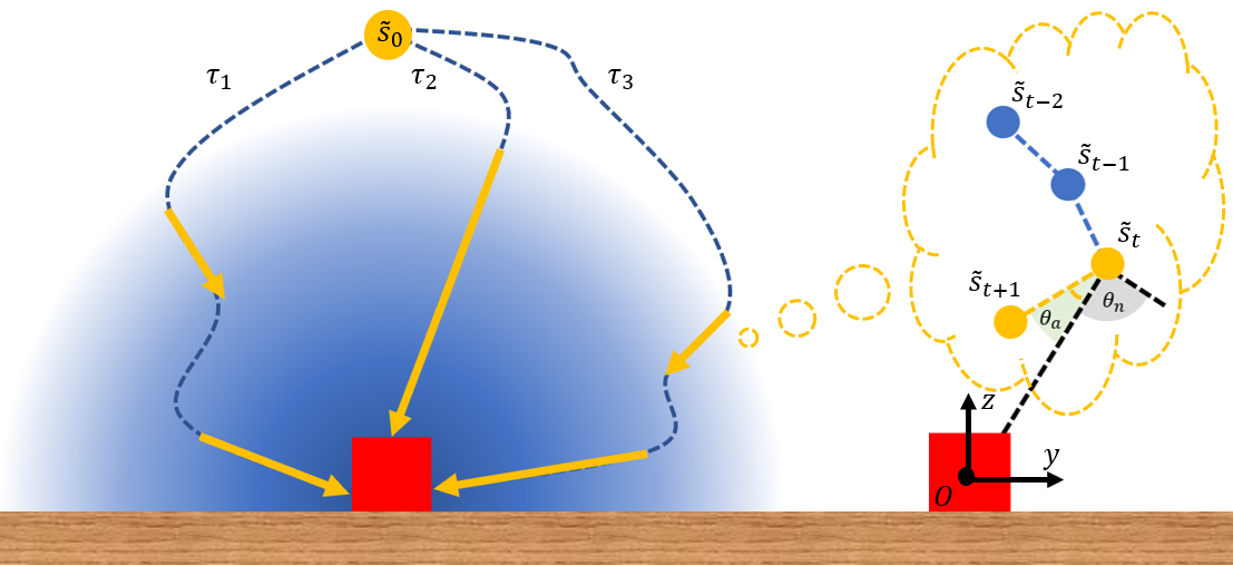
Figure 2: The blue gradient circle is the operator’s ideal reward function (true intent) where the inner portion is high reward and the outer portion is low reward. $\tau_{1},\tau_{2},\tau_{3}$ are complete trajectories of the approaching stage. $\theta_{a}$ is the approach angle between vectors ${\tilde{s}_{t}o}$ and ${\tilde{s}_{t}\tilde{s}_{t+1}}$, and $\theta_{n}$ is the noise angle to be set.

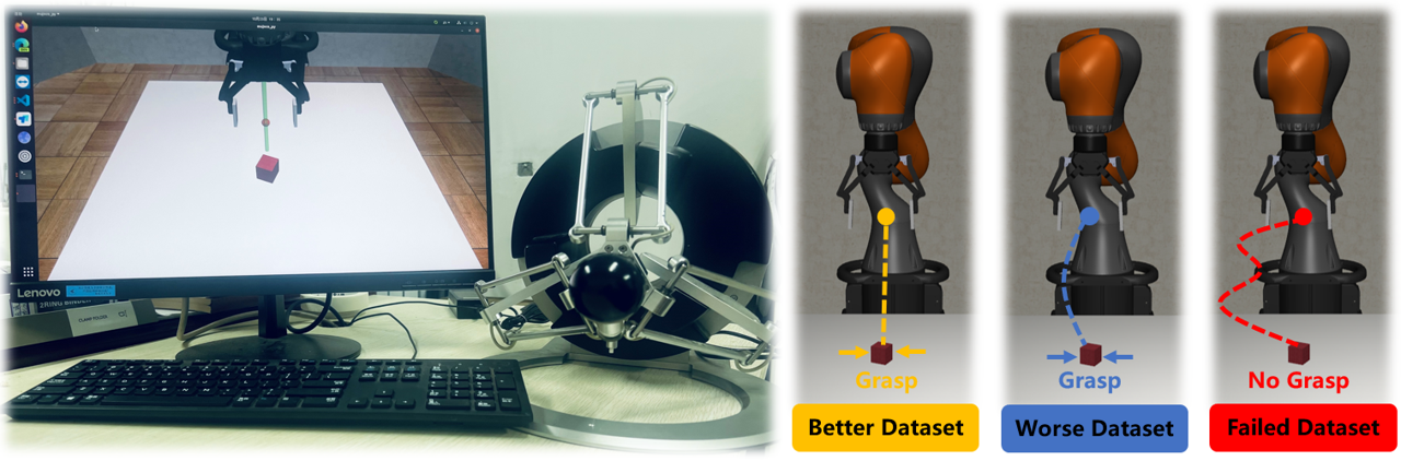
Figure 3: Teleoperation Demonstration System. Better datasets horizons: 100-150; Worse datasets horizons: 200-400; The failure of Failed datasets is due to inability to grasp target within 500 horizon range.

IV EXPERIMENTS

In this section, we experimentally answer the following questions. (1) Is there an optimal range of noise angle? (2) Does a fine-grained confidence scores evaluation of data improve performance more than simply filtering noisy data? (3) How does CIQL-A compare to CIQL-E and which algorithm is more aligned to human intent?

IV-A Experiments Setting

We develop a robotic teleoperation system using the input signaling capability of the Omega.3 haptic device to collect human demonstrations. Our system integrates seamlessly with Robosuite, which provides an IIWA robotic arm with an OSC-POSE controller. The control inputs contain a set of features including position vectors $\{x,y,z\}$, pitch, yaw, and roll angles $\{\theta_{p},\theta_{y},\theta_{r}\}$, and grasping binary signals $\{g\}$. We collect three types of human datasets at a control frequency of 20 Hz with a horizon limitation of 500: Better, Worse, and Failed. Each type consists of 30 trajectories with different horizons, as shown in Fig.3.

Our training hyperparameters are set as follows: the learning rates for both actors and critics are set to 5e-6, with a total training step of 500K. During training, we set the horizon to 200 and choose the moving average success rate of 10 trajectories as the metric for selecting the best model. During evaluation, we measure the average of the success rate for every 100 trajectories among 10 random seeds as the metric for evaluating the policy, with a set horizon of 500.

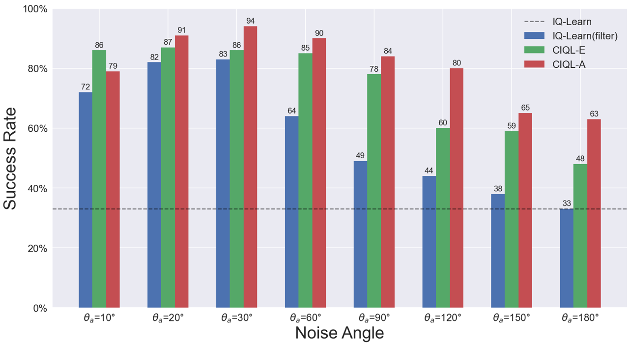
Figure 4: Effect of Noise Angle. We use the Better-Worse-Failed datasets (90) to explore the effect of noise angles on the success rates. IQ-Learn(filter) is learning on filtered noisy data, and it becomes IQ-Learn when $\theta_{a}$ equal to 180°.

TABLE I:

Datasets	IQ-Learn	IQ-Learn(filter)	CIQL-E	CIQL-A
Better(30)	66.9$\pm$4.7	86.4$\pm$3.3	84.4$\pm$3.4	86.9$\pm$4.0
Worse(30)	38.1$\pm$4.3	51.5$\pm$3.9	61.8$\pm$5.9	71.9$\pm$3.5
Better-Worse(30)	27.7$\pm$5.4	51.4$\pm$4.0	60.7$\pm$5.2	91.9$\pm$1.4
Better-Failed(30)	57.0$\pm$5.7	78.3$\pm$4.2	82.2$\pm$4.2	84.1$\pm$3.4
Worse-Failed(30)	32.4$\pm$5.4	62.5$\pm$4.3	67.6$\pm$4.5	65.9$\pm$5.5
Better-Worse-Failed(30)	47.3$\pm$4.6	76.0$\pm$6.2	71.7$\pm$4.8	81.0$\pm$4.2
Better-Worse-Failed(60)	41.3$\pm$5.3	87.8$\pm$3.0	70.9$\pm$3.3	94.0$\pm$2.2
Better-Worse-Failed(90)	32.9$\pm$4.9	64.2$\pm$4.6	85.0$\pm$2.8	90.3$\pm$2.1

IV-B Noise Angle Evaluation

As shown in Fig.4, we use a Better-Worse-Failed datasets (90 trajectories) to investigate the effect of a noise angle ranging from $10^{\circ}$ to $180^{\circ}$ on the success rate. The experimental results show that there exists an optimal noise angle $\theta_{noise}$ ranging from $20^{\circ}$ to $60^{\circ}$, which we refer to the optimal threshold.

It is important to note that when the noise angle is below the threshold, the algorithm’s performance improves as the noise angle increases. Conversely, when the noise angle is above the threshold, the performance declines as the noise angle increases. This phenomenon can be attributed to the fact that the threshold represents the true noise level in the data. Data above this threshold are real noise and has a negative impact on performance. The decrease of noise angle reduces the diversity of data, and when the noise angle is lower than the true noise level, it filters data that could potentially improve performance. Furthermore, algorithms that use our data confidence evaluation method can significantly improve performance at all angles and datasets, which highlights the strengths of our method. For instance, with the noise angle set to 30°, the success rate of CIQL(filter) is improved by $50\%$, CIQL-E by $53\%$, and CIQL-A by $60\%$ compared to the original algorithm..

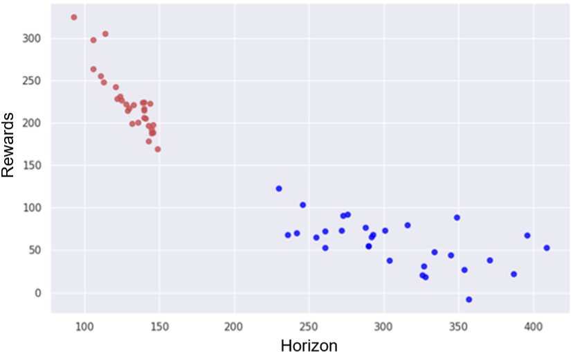
(a) CIQL-A

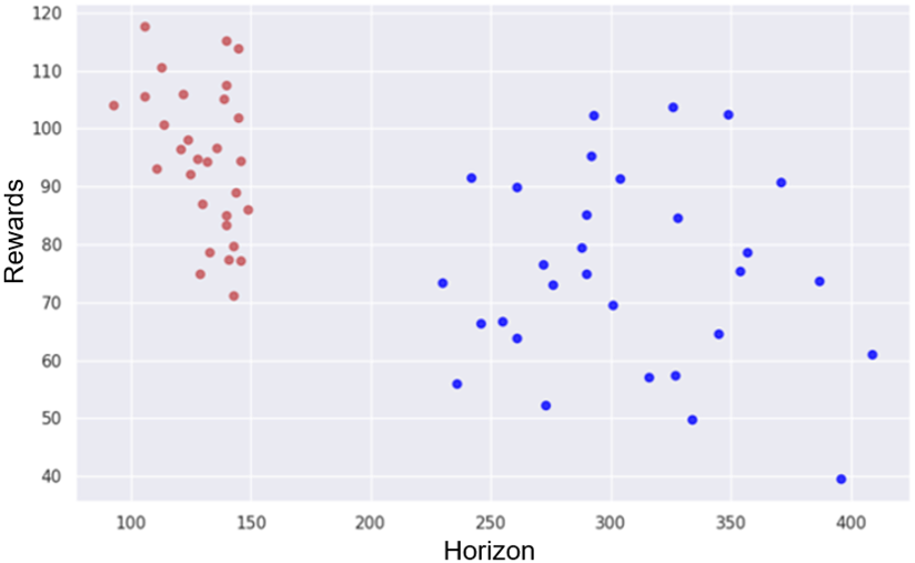
(b) CIQL-E

Figure 5: Evaluation of Trajectories. We evaluate the trajectories using the reward function recovered by the optimal Q-function learned in the Better-Worse-Failed datasets (90, $\theta$=60^∘). The left side of the figure shows the results of CIQL-A and the right side shows the results of CIQL-E, where the red points are the Better data and the blue points are the Worse data.

IV-C CIQL Evaluation

We investigate the performance of each algorithm using different datasets with the noise angle set to $60^{\circ}$, as shown in Table I. These datasets have the same number of components, such as 10 trajectories each for the Better, Worse, and Failed components in the Better-Worse-Failed dataset (30 trajectories). In most cases, the performance of the algorithms is ranked as CIQL-A($40.3\%$) $>$ CIQL-E($30.1\%$) $>$ CIQL(filter,$26.8\%$) $>$ IQ-Learn, based on the average success improvement over the original algorithm. Among them, CIQL-A has a $13.5\%$ improvement in success rate over IQ-Learn(filter). This shows that a fine-grained confidence scores evaluation of data is more effective than simply filtering noisy data. However, when the noise angle is set to a smaller value, some optimal data may be incorrectly identified as noise. This has a negative impact on the performance of CIQL-A. In such cases, CIQL-E actually outperforms CIQL-A, as in Fig.4 for a noise angle of 10°.

The horizon of a trajectory can indicate a human’s performance, specifically, the shorter horizon, the better its performance. We evaluate the human trajectories using the cumulative reward $\eta_{\tau_{i}}=\sum_{t=0}^{h_{i}}\gamma^{t}r(s_{t},a_{t})$. As shown in Fig. 5, the reward function inferred by CIQL-A aligns more closely with human intent. This is because CIQL-E simply filters noisy data, and noisy data does not contribute to the training of the reward function. On the other hand, CIQL-A’s reward function penalizes noisy data, leading to a reward function that more closely aligns human intent.

V CONCLUSIONS

Summary. We develop a framework to use confidence scores on the IQ-Learn algorithm and propose a dynamics-based method to evaluate the data confidence scores. The method uses transitions to calculate the approach angle and divides the data into useful and noisy data by setting the noise angle. Then use a confidence function to evaluate the useful data with a fine-grained confidence score. We experimentally explore the effect of the noise angle on the success rate to obtain the optimal threshold (true noise) and the results show that our confidence setting improves the algorithm’s performance. Furthermore, we find that penalizing noisy data is more effective than just filtering them. As well as the reward function recovered in this way is also more aligned to human intent.

Limitation and Future Work. Although our data confidence evaluation method can improve the performance, they are sensitive to the choice of noise angles. Therefore, it is an interesting topic to find the effective noise angles quickly. One way to recognize noise when approaching an object is to set the noise angle. However, the challenge lies in recognizing noise when approaching an object while also avoiding obstacles. In confidence-based imitation learning, it is critical to explore the true confidence score of the data or to make imitation learning more robust.

References

- [1] L. Pinto and A. Gupta, “Supersizing self-supervision: Learning to grasp from 50k tries and 700 robot hours,” in 2016 IEEE international conference on robotics and automation (Learning From Imperfect Demonstrations From). IEEE, 2016, pp. 3406–3413.
- [2] A. Mandlekar, D. Xu, J. Wong, S. Nasiriany, C. Wang, R. Kulkarni, L. Fei-Fei, S. Savarese, Y. Zhu, and R. Martín-Martín, “What matters in learning from offline human demonstrations for robot manipulation,” arXiv preprint arXiv:2108.03298, 2021.
- [3] M. Beliaev, A. Shih, S. Ermon, D. Sadigh, and R. Pedarsani, “Imitation learning by estimating expertise of demonstrators,” in International Conference on Machine Learning. PMLR, 2022, pp. 1732–1748.
- [4] A. Mandlekar, J. Booher, M. Spero, A. Tung, A. Gupta, Y. Zhu, A. Garg, S. Savarese, and L. Fei-Fei, “Scaling robot supervision to hundreds of hours with roboturk: Robotic manipulation dataset through human reasoning and dexterity,” in 2019 IEEE/RSJ International Conference on Intelligent Robots and Systems (IROS). IEEE, 2019, pp. 1048–1055.
- [5] V. Tangkaratt, B. Han, M. E. Khan, and M. Sugiyama, “Vild: Variational imitation learning with diverse-quality demonstrations,” arXiv preprint arXiv:1909.06769, 2019.
- [6] D. Brown, W. Goo, P. Nagarajan, and S. Niekum, “Extrapolating beyond suboptimal demonstrations via inverse reinforcement learning from observations,” in International conference on machine learning. PMLR, 2019, pp. 783–792.
- [7] D. S. Brown, W. Goo, and S. Niekum, “Better-than-demonstrator imitation learning via automatically-ranked demonstrations,” in Conference on robot learning. PMLR, 2020, pp. 330–359.
- [8] L. Chen, R. Paleja, and M. Gombolay, “Learning from suboptimal demonstration via self-supervised reward regression,” in Conference on robot learning. PMLR, 2021, pp. 1262–1277.
- [9] Y. Wang, C. Xu, B. Du, and H. Lee, “Learning to weight imperfect demonstrations,” in International Conference on Machine Learning. PMLR, 2021, pp. 10 961–10 970.
- [10] Y.-H. Wu, N. Charoenphakdee, H. Bao, V. Tangkaratt, and M. Sugiyama, “Imitation learning from imperfect demonstration,” in International Conference on Machine Learning. PMLR, 2019, pp. 6818–6827.
- [11] S. Zhang, Z. Cao, D. Sadigh, and Y. Sui, “Confidence-aware imitation learning from demonstrations with varying optimality,” Advances in Neural Information Processing Systems, vol. 34, pp. 12 340–12 350, 2021.
- [12] D. P. Kingma, S. Mohamed, D. Jimenez Rezende, and M. Welling, “Semi-supervised learning with deep generative models,” Advances in neural information processing systems, vol. 27, 2014.
- [13] D. A. Pomerleau, “Alvinn: An autonomous land vehicle in a neural network,” Advances in neural information processing systems, vol. 1, 1988.
- [14] M. Bain and C. Sammut, “A framework for behavioural cloning.” in Machine Intelligence 15, 1995, pp. 103–129.
- [15] S. Schaal, “Is imitation learning the route to humanoid robots?” Trends in cognitive sciences, vol. 3, no. 6, pp. 233–242, 1999.
- [16] S. Ross and D. Bagnell, “Efficient reductions for imitation learning,” in Proceedings of the thirteenth international conference on artificial intelligence and statistics. JMLR Workshop and Conference Proceedings, 2010, pp. 661–668.
- [17] P. Abbeel and A. Y. Ng, “Apprenticeship learning via inverse reinforcement learning,” in Proceedings of the twenty-first international conference on Machine learning, 2004, p. 1.
- [18] U. Syed, M. Bowling, and R. E. Schapire, “Apprenticeship learning using linear programming,” in Proceedings of the 25th international conference on Machine learning, 2008, pp. 1032–1039.
- [19] B. D. Ziebart, A. L. Maas, J. A. Bagnell, A. K. Dey et al., “Maximum entropy inverse reinforcement learning.” in Aaai, vol. 8. Chicago, IL, USA, 2008, pp. 1433–1438.
- [20] T. Xu, Z. Li, and Y. Yu, “Error bounds of imitating policies and environments,” Advances in Neural Information Processing Systems, vol. 33, pp. 15 737–15 749, 2020.
- [21] J. Ho and S. Ermon, “Generative adversarial imitation learning,” Advances in neural information processing systems, vol. 29, 2016.
- [22] J. Fu, K. Luo, and S. Levine, “Learning robust rewards with adversarial inverse reinforcement learning,” arXiv preprint arXiv:1710.11248, 2017.
- [23] N. Baram, O. Anschel, I. Caspi, and S. Mannor, “End-to-end differentiable adversarial imitation learning,” in International Conference on Machine Learning. PMLR, 2017, pp. 390–399.
- [24] D. Garg, S. Chakraborty, C. Cundy, J. Song, and S. Ermon, “Iq-learn: Inverse soft-q learning for imitation,” Advances in Neural Information Processing Systems, vol. 34, pp. 4028–4039, 2021.
- [25] H. Xiao, M. Herman, J. Wagner, S. Ziesche, J. Etesami, and T. H. Linh, “Wasserstein adversarial imitation learning,” arXiv preprint arXiv:1906.08113, 2019.
- [26] T. Haarnoja, A. Zhou, P. Abbeel, and S. Levine, “Soft actor-critic: Off-policy maximum entropy deep reinforcement learning with a stochastic actor,” in International conference on machine learning. PMLR, 2018, pp. 1861–1870.
- [27] Z. Cao and D. Sadigh, “Learning from imperfect demonstrations from agents with varying dynamics,” IEEE Robotics and Automation Letters, vol. 6, no. 3, pp. 5231–5238, 2021.
- [28] P. S. Castro, S. Li, and D. Zhang, “Inverse reinforcement learning with multiple ranked experts,” arXiv preprint arXiv:1907.13411, 2019.