Incremental Exponential Stability of the Unidirectional Flow Model

Abstract

Incremental stability is assessed for the Unidirectional Flow Model, which describes the flow of a conserved quantity in a cascade of compartments. The model is governed by a cooperative system of nonlinear ordinary differential equations with a right-hand side that depends on an input function. Suitable conditions are given on the input function such that the solutions to the model converge to each other at an exponential rate. Milder conditions, compared with the latter, are given such that the solutions to the model converge to each other asymptotically. These conditions are related to inflow-connected and outflow-connected compartmental systems and are easy to check. Computational means to estimate the exponential rate are given and tested against numerical solutions of the model. A natural application of incremental stability is state estimation, demonstrated in the numerical experiments, put into a traffic flow context.

Compartmental systems. Cooperative differential equations. Incremental Exponential Stability. Traffic flow models. State estimation.

1 Introduction

Mass conservation laws govern an abundance of dynamical systems. Examples of such dynamical systems include (but are not limited to) macroscopic traffic flow models [8, 22, 21, 20], epidemiological models [15, 14], biological systems describing blood glucose [4] or the flow of ribosomes [19], and even probabilistic models like Markov chains [26, ch. 12]. In this paper, we consider the Unidirectional Flow Model (UFM), which describes the flow of a conserved quantity in a cascade of compartments. This model is governed by Ordinary Differential Equations (ODEs) and is a particular instance of the Traffic Reaction Model [22], and the Ribosome Flow Model [19]. Our goal is to obtain mathematical insight into the UFM that will be valuable for state estimation.

The UFM belongs to the class of ODEs called compartmental systems, which describes the flow of a conserved quantity between so-called compartments [12]. Compartmental systems are, in general, nonlinear and time-varying, and several authors have studied their asymptotic behavior. Asymptotic stability of the origin and the related concept of washout was considered in [10]. Sufficient criteria for the existence, uniqueness, and asymptotic stability of equilibrium points and periodic solutions were proposed in [23]. Under mild conditions, [17] showed that time-invariant compartmental systems do not admit periodic solutions. Quite general criteria for asymptotic stability of the origin for linear time-varying compartmental systems are given in [3]. Besides the linear case (with the exception of [10]), the convergence rate for these asymptotic behaviors has not received much attention. Research efforts related to systems and control have also been conducted, e.g., congestion control for nonlinear compartmental systems, and for linear compartmental systems, positive state observers were considered in [25] and optimal control in [6].

A second class of systems that categorizes the UFM is monotone dynamical systems [24]. Specifically, the UFM is governed by a cooperative system of ODEs, a particular case of monotone dynamical systems that have been studied in several aspects concerning stability. To conclude the asymptotic stability of the origin of monotone systems, the construction of separable Lyapunov functions was introduced in [9]. Separable Lyapunov functions were also constructed in [7] for monotone systems via a contractive approach. The solutions to contractive systems approach each other exponentially [16], and this concept was used in [13] to show incremental stability [1] for monotone systems. Moreover, contractive systems were generalized in [18] for time-varying nonlinear systems (not necessarily monotone) to handle small transients, where one illustrative example is a ribosome flow model. Contraction analysis was successfully applied in [27] for a generalized ribosome flow model capable of modeling several realistic features of the translation process.

The main contribution of this paper is to show that the UFM is incrementally exponentially stable in its entire state space with respect to an appropriate set of input functions. This means that for a fixed set of model parameters and an appropriate input function, all of the solutions to the UFM approach each other at an exponential rate. A formula for an estimate of the exponential rate is given, and in the numerical experiments, we verify that the solutions to the UFM approach each other at this rate. The numerical experiments are put into a traffic density estimation context to demonstrate a practical use case of the main contribution. In [19], the rate of convergence to equilibria of the Ribosome Flow Model was stated as unknown. The UFM is a special case of the Ribosome Flow Model, and convergence to equilibria follows from incremental exponential stability. Since we provide means to estimate the exponential rate, we have partially solved an open problem.

The paper is structured as follows. In Section 2, we define incremental exponential stability and the class of differential equations called cooperative systems. In Section 3.1, we introduce the UFM and show some of its salient properties. In Section 3.2, we provide suitable conditions for the solutions to the UFM to converge to each other exponentially, from which incremental exponential stability directly follows in a corollary. In Section 4, we put the main results into the context of traffic density estimation and verify the convergence rate between the solutions via numerical experiments. In Section 5, we conclude the results and highlight future research directions. The proofs that we consider important are included in the main body of the paper, and the others are put in the Appendix.

Notation: Let $\mathbb{N}\coloneqq\{1,2,\dots\}$ and $\mathbb{N}_{0}\coloneqq\mathbb{N}\cup\{0\}$. We denote Euclidean space by $\mathbb{R}^{n}$ and set $\mathbb{R}^{n}_{+}\coloneqq[0,+\infty)^{n}$ and $\mathbb{R}^{n}_{++}\coloneqq(0,+\infty)^{n}$. For any $x,y\in\mathbb{R}^{n}$ we write $x\leq y$ and $x\ll y$ if $y-x\in\mathbb{R}^{n}_{+}$ and $x-y\in\mathbb{R}^{n}_{++}$, respectively. If $x\leq y$ and $x\neq y$, we write $x<y$. We denote the $p$-norm by $|\cdot|_{p}:\mathbb{R}^{n}\to\mathbb{R}_{+}$ which is defined by $|x|_{p}^{p}=\sum_{i=1}^{n}|x_{i}|^{p}$ for $p\in[1,+\infty)$ and by $|x|_{\infty}=\max_{i}|x_{i}|$ for $p=+\infty$. Moreover, we denote $\langle x,y\rangle\coloneqq\sum_{i=1}^{n}x_{i}y_{i}$ for all $x,y\in\mathbb{R}^{n}$. If $I$ is an interval in $\mathbb{R}$, we denote its length by $|I|$.

2 Incremental Exponential Stability and Cooperative Systems

The major property of interest in this paper is the incremental exponential stability of finite-dimensional dynamical systems. This property implies that some or all of the solutions to a system, given fixed input and model parameters, approach each other exponentially in a normed sense. In this work, we consider incremental exponential stability of dynamical systems governed by a system of ODEs. Let $n,m\geq 1$ be integers, $a,b\in\mathbb{R}^{n}$,

$$\begin{split}\mathcal{X}&\coloneqq\{x\in\mathbb{R}^{n}:a\leq x\leq b,\;a\ll b\},\text{ and }\\ \mathcal{U}&\coloneqq\{v:\mathbb{R}\to\mathbb{R}^{m}\;:\text{ $v$ is continuous and bounded}\}.\end{split}$$ (1)

The differential equation under consideration is

$$\dot{x}(t)=f(x(t),u(t)),$$ (2)

where $f:\mathbb{R}^{n}\times\mathbb{R}^{m}\to\mathbb{R}^{n}$. It is assumed that for all $(\xi,u)\in\mathcal{X}\times\mathcal{U}$, system (2) admits a unique solution $x$, such that $x(0)=\xi$, $x(t)$ is defined for all $t\geq 0$, and $x(t)\in\mathcal{X}$ for all $t\geq 0$. In the next section, we discuss a class of systems for which this assumption holds. Given the input function $u\in\mathcal{U}$ and initial value $\xi\in\mathcal{X}$, we denote when convenient, the solution to (2) at time $t$ by $\phi(t,\xi,u)$, where $\phi(0,\xi,u)=\xi$.

Taking inspiration from [2, Definition 2.1], we define the incremental exponential stability for system (2).

Definition 1 (Incremental exponential stability)

Let $\mathcal{X}_{\text{s}}$ and $\mathcal{U}_{\text{s}}$ be non-empty and fixed subsets of $\mathcal{X}$ and $\mathcal{U}$, respectively. The system (2) is incrementally exponentially stable (IES) in $\mathcal{X}_{\text{s}}$ with respect to $\mathcal{U}_{\text{s}}$, if there exist $\lambda>0$ and $\gamma\geq 1$, such that for all $\xi^{1},\xi^{2}\in\mathcal{X}_{\text{s}}$, $u\in\mathcal{U}_{\text{s}}$, and $t\geq 0$

$$|\phi(t,\xi^{1},u)-\phi(t,\xi^{2},u)|_{1}\leq\gamma e^{-\lambda t}|\xi^{1}-\xi^{2}|_{1}.$$ (3)

Fix any $\lambda>0$ and $\gamma\geq 1$. Then the system (2) is IES in $\mathcal{X}_{\mathrm{s}}$ with respect to $\mathcal{U}_{\mathrm{s}}$ for $(\lambda,\gamma)$, if (3) holds for all $\xi^{1},\xi^{2}\in\mathcal{X}$, $u\in\mathcal{U}_{\mathrm{s}}$, and $t\geq 0$.

Remark 1

Incremental exponential stability can be useful in the context of state estimation. Suppose (2) is IES in $\mathcal{X}$ with respect to $\mathcal{U}$, and both $f$ and $u$ are known. Then, for each fixed $u\in\mathcal{U}$, the long-term behavior of the solutions to the system (2) is independent of the initial condition. This means from a state estimation perspective that for any $\xi^{1}\in\mathcal{X}$, the solution $\phi(t,\xi^{1},u)$ can be estimated by $\phi(t,\xi^{2},u)$ for arbitrary $\xi^{2}\in\mathcal{X}$, with the guarantee that that the estimation error $t\mapsto|\phi(t,\xi^{1},u)-\phi(t,\xi^{2},u)|_{1}$ approaches zero at an exponential rate.

A central class of systems in this paper is cooperative differential equations [24, ch. 3]. First, we briefly describe what it means for a system of ordinary differential equations to be cooperative and then define this notion for system (2). Consider the following system

$$\dot{x}(t)=F(t,x(t)),$$ (4)

where $F:\mathbb{R}\times D\to\mathbb{R}^{n}$ is continuous and continuously differentiable with respect to its second argument and $D\subset\mathbb{R}^{n}$ is open. Fix any $x_{0},y_{0}\in D$ with $x_{0}\leq y_{0}$ and let $x$, $y$ be the solutions to (4) with $x(0)=x_{0},$ $y(0)=y_{0}$. For simplicity, suppose both $x$ and $y$ are defined on $[0,+\infty)$, then (4) is said to be cooperative if

$$x(t)\leq y(t)\text{ for all }t\geq 0.$$ (5)

We will now extend the notion of cooperative differential equations for system (2).

Definition 2

Let $\mathcal{U}_{\mathrm{c}}$ be a fixed, non-empty subset of $\mathcal{U}$. The system (2) is cooperative for inputs in $\mathcal{U}_{\mathrm{c}}$ if for each fixed $u\in\mathcal{U}_{\mathrm{c}}$ and for all $\xi^{1},\xi^{2}\in\mathcal{X}$ with $\xi^{1}\leq\xi^{2}$,

$$\phi(t,\xi^{1},u)\leq\phi(t,\xi^{2},u)\text{ for all $t\geq 0$}.$$ (6)

In the sequel, we will discuss incremental exponential stability for the Unidirectional Flow Model (UFM)—a system that is cooperative for all inputs of interest.

3 The Unidirectional Flow Model (UFM)

In Section 3.1 we define the UFM, describe its physical interpretation, and state some of its mathematical properties. It is shown in Section 3.2 that there exists a set of input functions $U_{\mathrm{s}}$ such that the UFM is IES in the whole state space with respect to $U_{\mathrm{s}}$.

3.1 Model Description

The Unidirectional Flow Model describes a conserved quantity in a string of two or more connected compartments. Let the integer $n\geq 2$ denote the number of compartments and $t\mapsto x(t)\coloneqq(x_{1}(t),\dots,x_{n}(t))$ the conserved quantity in the system over time. In particular, $0\leq x_{i}(t)\leq c$ denotes the amount of the conserved quantity in compartment $i$ at time $t\geq 0$, where the real number $c>0$ denotes capacity. All compartments have the same capacity $c$. The flow from compartment $i$ to compartment $i+1$ is governed by the relation

$$F_{i}(t)\coloneqq wx_{i}(t)(c-x_{i+1}(t)),\quad i=1,\dots,n-1,$$ (7)

where the real number $w>0$ is a rate coefficient. At the boundary compartments $1$ and $n$ there is an exchange of the conserved quantity with what is usually referred to as the environment: the inflow $F_{1}(t)$ from the environment to compartment $1$ and the outflow $F_{n}(t)$ from compartment $n$ to the environment

$$\begin{split}F_{0}(t)&\coloneqq wu_{1}(t)(c-x_{1}(t)),\\ F_{n}(t)&\coloneqq wx_{n}(t)(c-u_{2}(t)),\end{split}$$ (8)

where $u\coloneqq(u_{1},u_{2}):\mathbb{R}\to[0,c]^{2}$ is a continuous function governed by external factors. We refer to $u$ as the input function, which serves as a valve mechanism. If $u_{1}(t)=0$, then the inflow $F_{0}(t)=0$, and if $u_{2}(t)=c$, then the outflow $F_{n}(t)=0$. Each compartment $i$ has exactly one inflow $F_{i-1}(t)$ and exactly one outflow $F_{i}(t)$, which leads to the conservation law

$$\dot{x}_{i}(t)=F_{i-1}(t)-F_{i}(t),\quad t\geq 0.$$ (9)

The compartments and associated flows are illustrated in Fig 1.

Figure 1: This is a conceptual illustration of the Unidirectional Flow Model. The circles denote compartments whereas the arrows denote flows. Above is a diagram of the overall system and below is a diagram of an arbitrary compartment to associate the flows defined in (7) and (8) with the corresponding arrows.

The UFM is governed by the conservation law (9) with the flows (7), (8) and will be written as

$$\dot{x}(t)=f(x(t),u(t)).$$ (F)

For this differential equation, we define the state space $C$ and input space $U$ by

$$\begin{split}C&\coloneqq[0,c]^{n}\text{ and }\\ U&\coloneqq\{u:\mathbb{R}\to\mathbb{[}0,c]\;:\;\text{$u$ is continuous}\}.\end{split}$$ (10)

The map $f:\mathbb{R}^{n}\times\mathbb{R}^{2}\to\mathbb{R}^{n}$ is given by

$$f_{i}(x,u)\coloneqq wx_{i-1}(c-x_{i})-wx_{i}(c-x_{i+1})$$ (11)

where $i=1,\dots,n$, $\;x_{0}\coloneqq u_{1}$, and $x_{n+1}\coloneqq u_{2}$. For a summary of the model parameters associated with (F), see Table 1.

Table 1: Model parameters associated with (F)

Variable	Value	Meaning
$n$	$\geq 2$, integer	number of compartments
$c$	$>0$, real	capacity
$w$	$>0$, real	rate coefficient

Throughout this paper, the model parameters $n$, $c$, and $w$ in Table 1, are considered fixed and arbitrary unless stated otherwise. Given these parameters, we exclusively consider solutions to (F) for $f$ given by (11), initialized at time $t=0$, with initial values $\xi\in C$ and input functions $u\in U$. In 3 in the Appendix we show that for all $(\xi,u)\in C\times U$, system (F) admits a unique solution $x$, such that $x(0)=\xi$, $x(t)$ is defined for all $t\geq 0$, and $x(t)\in C$ for all $t\geq 0$. When convenient we denote the solution to (F) by $\phi(t,\xi,u)$, where $\phi(0,\xi,u)=\xi$, to signify the initial value $\xi$ and input function $u$.

Two additional properties of system (F) are proved in the Appendix. In 4, we show that (F) is cooperative for inputs in $U$. And in 5, we show that (F) inherits the following property. Fix any $u\in U$ and suppose $x$ satisfies (F). Then $y$ defined by $y_{i}\coloneqq c-x_{n+1-i}$, $i\in\{1,\dots,n\}$, satisfies (F) with the input function $v\coloneqq(c-u_{2},c-u_{1})$. Since $x_{i}$ denotes the amount of the conserved quantity over time in a compartment with a designated capacity, it can also be interpreted as occupied space. In contrast, $y_{i}$ denotes the free-space, or available space, in compartment $n+1-i$ over time. Both of these properties are used frequently in the proofs to come.

For the remainder of this section, we will discuss the solutions to (F) while imposing certain criteria on the input function $u\in U$. In this regard, we define the terms closed, outflow-connected, and inflow-connected.

Definition 3

Consider the system (F) for some input function $u\in U$. Fix any interval $I\subset[0,+\infty)$ and real number $\alpha\in(0,c]$. Then the system (F) is said to be closed on $I$ if

$$u(t)=(0,c),\quad t\in I,$$ (12)

inflow-connected on $I$ if

$$u_{1}(t)\geq\alpha,\quad t\in I,$$ (13)

and outflow-connected on $I$ if

$$u_{2}(t)\leq c-\alpha,\quad t\in I.$$ (14)

Remark 2

Our definition of outflow-connected deviates slightly from the definition given in the seminal paper [12]. Here, a compartmental system is outflow-connected if there is a path from each compartment to a compartment with an outflow to the environment. We do not include this in the definition because it is always the case for the UFM, as can be seen in the Fig 1.

To elaborate on the Definition 3, let $x(t)\coloneqq\phi(t,\xi,u)$ be the solution to (F) for some $\xi\in C$ and $u\in U$. If the system (F) is closed on $I$, then the the total conserved quantity $t\mapsto\sum_{i=1}^{n}x_{i}(t)$ is constant on $I$, because for all $t\in I$, $u_{1}(t)=0$, $u_{2}(t)=c$, and

$$\sum_{i=1}^{n}\dot{x}_{i}(t)=wu_{1}(t)(c-x_{1}(t))-wx_{n}(t)(c-u_{2}(t))=0.$$ (15)

On the other hand, the total conserved quantity is subject to change on the interval $I$ if (F) is either inflow-connected or outflow-connected on $I$. Indeed, in this case the inflow $wu_{1}(t)(c-x_{1}(t))$ and outflow $wx_{n}(t)(c-u_{2}(t))$ are not necessarily equal.

We further elaborate on the consequence of outflow-connected by providing a preliminary result, which will be important in the sequel. Suppose (F) is outflow-connected on some interval $I\coloneqq[t_{0},t_{1}]\subset[0,+\infty)$ for some $\alpha\in(0,c]$, i.e.

$$u_{2}(t)\in[0,c-\alpha],\quad t\in[t_{0},t_{1}].$$ (16)

We show that if $t_{1}$ is large enough, then there exists a time $\tau\coloneqq t_{0}+h\in[t_{0},t_{1})$ and real numbers $s_{1},\dots,s_{n}\in(0,c)$ such that the $x_{i}$ satisfy

$$x_{i}(t)\in[0,c-s_{i}],\quad t\in[\tau,t_{1}].$$ (17)

Put differently, at times $\tau$ all compartments are non-full and remain non-full on the interval $[\tau,t_{1}]$ according to the inclusion (17). We prove this claim in the following lemma, where we give expressions for $h$ and the $s_{i}$.

Lemma 1

Fix any $\alpha\in(0,c]$ and $p\in(0,1)$. Define $\epsilon\coloneqq(\epsilon_{0},\dots,\epsilon_{n})\in(0,c]\times(0,c)^{n}$ and $h\geq 0$ by

$$\begin{split}\epsilon_{0}&\coloneqq\alpha,\quad\epsilon_{i}\coloneqq p\frac{\epsilon_{i-1}c}{\epsilon_{i-1}+c},\quad i=1,\dots,n,\\ h&\coloneqq-\sum_{i=1}^{n}\frac{\ln(1-p)}{w(\epsilon_{i-1}+c)}.\end{split}$$ (18)

Consider system (F) and let $(\xi,u)\in C\times U$ be fixed but arbitrary. Let $t_{0}\geq 0$ and $t_{1}>t_{0}+h$. If

$$u_{2}(t)\leq c-\alpha,\quad t\in[t_{0},t_{1}],$$ (19)

then for all $t\in[t_{0}+h,t_{1}]$

$$\phi_{i}(t,\xi,u)\in[0,c-\epsilon_{n+1-i}],\quad i=1,\dots,n.$$ (20)

Proof 3.1.

It follows from the definition of $\epsilon,h$ and $\alpha$ that $\epsilon\in(0,c]\times(0,c)^{n}$ and $h\geq 0$. Following 3 in the Appendix, since $(\xi,u)\in C\times U$, where $C$ and $U$ are given in (10), it holds that for all $i=1,\dots,n$ and $t\geq 0$, $\phi_{i}(t,\xi,u)\in[0,c]$. Let then $x:[0,+\infty)\to\mathbb{R}^{n}$ be defined by

$$x_{i}(t)\coloneqq c-\phi_{n+1-i}(t,\xi,u),\quad t\geq 0,\quad i=1,\dots,n.$$ (21)

Thus, we have $x_{i}(t)\in[0,c]$ for $i=1,\dots,n$. Let us now prove that $x_{i}(t)\geq\epsilon_{i}$ for $i=1,\dots,n$ and $t\in[t_{0}+h,t_{1}]$.

For convenience we write $x_{0}\coloneqq c-u_{2}$ and $x_{n+1}\coloneqq c-u_{1}$. Define then $a_{i}\coloneqq w(c+\epsilon_{i-1})$ and $b_{i}\coloneqq\epsilon_{i}/p$ for any $i\in\{1,\dots,n\}$. Finally, let $\tau_{0}\coloneqq t_{0}$ and $\tau_{1},\dots,\tau_{n}$ be defined according to

$$\tau_{i}\coloneqq t_{0}-\sum_{k=1}^{i}\frac{\ln(1-p)}{a_{k}},$$ (22)

and consider for $i\in\{0,1,\dots,n\}$ the claim

$$P_{i}:\quad x_{i}(t)\geq\epsilon_{i}\text{ for all }t\in[\tau_{i},t_{1}].$$ (23)

By (19), $x_{0}(t)=c-u_{2}(t)\geq\alpha$ for all $t\in[t_{0},t_{1}]$. Hence, $P_{0}$ holds for $\epsilon_{0}=\alpha$. For $i\in\{1,\dots,n\}$, let us now assume that $P_{i-1}$ holds. By differentiating (21) and using $P_{i-1}$ and the fact that $x_{i+1}(t)\geq 0$, we get for any $t\in[\tau_{i-1},t_{1}]$,

$$\begin{split}\dot{x}_{i}(t)=&wx_{i-1}(t)(c-x_{i}(t))\\ &-wx_{i}(t)c+wx_{i}(t)x_{i+1}(t)\\ \geq&w\epsilon_{i-1}(c-x_{i}(t))-wx_{i}(t)c\\ =&w(c+\epsilon_{i-1})\Big{(}\frac{\epsilon_{i-1}c}{\epsilon_{i-1}+c}-x_{i}(t)\Big{)}\\ \eqqcolon&a_{i}(b_{i}-x_{i}(t)).\end{split}$$ (24)

Take then $r_{i}\coloneqq b_{i}-x_{i}$. We obtain for any $t\in[\tau_{i-1},t_{1}]$, $\dot{r}_{i}(t)=-\dot{x}_{i}(t)\leq-a_{i}r_{i}(t)$, which gives, by virtue of Grönwall’s inequality and using that $x_{i}(\tau_{i-1})\geq 0$,

$$r_{i}(t)\leq e^{-a_{i}(t-\tau_{i-1})}r_{i}(\tau_{i-1})\leq b_{i}e^{-a_{i}(t-\tau_{i-1})}$$ (25)

for all $t\in[\tau_{i-1},t_{1}]$. In turn, this yields (by definition of $r_{i}$) that for any $t\in[\tau_{i-1},t_{1}]$, $x_{i}(t)\geq l_{i}(t)$, where for $t\geq 0$ we define $l_{i}(t)\coloneqq b_{i}(1-e^{-a_{i}(t-\tau_{i-1})})$. In particular, note that $l_{i}(\tau_{i})=b_{i}(1-e^{-a_{i}(\tau_{i}-\tau_{i-1})})=b_{i}p=\epsilon_{i}$. Since $l_{i}$ is a strictly increasing function and noting that $\tau_{i-1}<\tau_{i}\leq t_{0}+h<t_{1}$, we then conclude that

$$x_{i}(t)\geq l_{i}(t)\geq l_{i}(\tau_{i})=\epsilon_{i}\text{ for all }t\in[\tau_{i},t_{1}],$$ (26)

thus proving that $P_{i}$ holds. We can therefore conclude that $P_{i}$ holds for any $i\in\{0,1,\dots,n\}$. Noting then that $t_{0}=\tau_{1}<\tau_{2}<\dots<\tau_{n}=t_{0}+h<t_{1}$, we can deduce that for any $i\in\{1,\dots,n\}$, and for any $t\in[t_{0}+h,t_{1}]$, $x_{i}(t)\in[\epsilon_{i},c]$, which, by definition of $x_{i}$, allows us to conclude that $\phi_{i}(t,\xi,u)\in[0,c-\epsilon_{n+1-i}]$ for any $t\in[t_{0}+h,t_{1}]$.

We end this section with a remark on the formulae (18) for $h$ and the $\epsilon_{i}$ which depends on the free parameter $p\in(0,1)$. The time $\tau\coloneqq t_{0}+h$ can be made arbitrarily close $t_{0}$ by choosing $p>0$ sufficiently small. This means in consequence that the $\epsilon_{i}>0$ become close to zero. In the next section, where we address incremental exponential stability for (F), Lemma 1 plays a central role.

3.2 Stability Analysis

In this section, we analyze the stability of the solutions to (F) with respect to each other, in the sense of bounding $|\phi(t,\xi^{1},u)-\phi(t,\xi^{2},u)|_{1}$ from above. The analysis is used to characterize a set $U_{\mathrm{s}}\subset U$ such that system (F) is IES in $C$ with respect to $U_{s}$. We also provide a milder assumption on the input function $u$ (compared with $u\in U_{\mathrm{s}}$), which guarantees $|\phi(t,\xi^{1},u)-\phi(t,\xi^{2},u)|_{1}\to 0$ as $t\to+\infty$ for all initial values $\xi^{1},\xi^{2}\in C$.

Let $x^{1}(t)\coloneqq\phi(t,\xi^{1},u)$ and $x^{2}(t)\coloneqq\phi(t,\xi^{2},u)$ be the solutions to (F) for fixed but arbitrary $\xi^{1},\xi^{2}\in C$ and $u\in U$. We look for a suitable condition on $u$, such that for a prescribed interval $[t_{0},t_{1}]\subset[0,+\infty)$ of arbitrary length,

$$|x^{1}(t)-x^{2}(t)|_{1}\leq\gamma e^{-\lambda(t-t_{0})}|x^{1}(t_{0})-x^{2}(t_{0})|_{1}$$ (27)

for all $t\in[t_{0},t_{1}]$, where the real numbers $\lambda>0$ and $\gamma\geq 1$ are independent of $\xi^{1},\xi^{2},t_{0},t_{1}$. In Theorem 3.3 we show that (F) being inflow-connected or outflow-connected on $[t_{0},t_{1}]$ (cf. Definition 3) is a suitable condition. That is, there exists a real number $\alpha\in(0,c]$ such that

$$\text{i)}\;\;u_{1}(t) \geq\alpha,\quad t\in[t_{0},t_{1}],\text{ or}$$ (28)

$$\text{ii)}\;\;u_{2}(t) \leq c-\alpha,\quad t\in[t_{0},t_{1}].$$ (29)

Formulae for $\lambda$ and $\gamma$ will be stated in the theorem, where we also show that for arbitrary $u\in U$,

$$t\mapsto|x^{1}(t)-x^{2}(t)|_{1}\text{ is non-increasing.}$$ (30)

Before stating the main theorem we will briefly discuss how we intend to show that the criterion ii) implies the bound (27). The proof that i) implies (27) follows indirectly from the latter via the change of coordinates described in 5 in the Appendix. For ease of presentation, we assume $t_{0}=0$ and $\xi^{1}\leq\xi^{2}$. We then want to demonstrate that ii) implies the special case of (27), written as

$$|x^{1}(t)-x^{2}(t)|_{1}\leq\gamma e^{-\lambda t}|\xi^{1}-\xi^{2}|_{1},\quad t\in[0,t_{1}].$$ (31)

According to 4, (F) is cooperative for inputs in $U$. Since $u\in U$ and $\xi^{1}\leq\xi^{2}$, the solutions $x^{1}$ and $x^{2}$ satisfy

$$x^{1}(t)\leq x^{2}(t),\quad t\in[0,t_{1}].$$ (32)

In the previous section it was shown in Lemma 1 that if (F) is outflow-connected on $[0,t_{1}]$ for sufficiently large $t_{1}$, then there exist real numbers $0\leq h<t_{1}$ and $\epsilon_{1},\dots,\epsilon_{n}\in(0,c)$ such that the solution $x$ of (F), satisfies $0\leq x_{i}(t)\leq c-\epsilon_{n+1-i}\eqqcolon c-s_{i}$ for all $t\in[h,t_{1}]$. Let $s_{n+1}\coloneqq\alpha$, then for all $t\in[h,t_{1}]$ and $i=1,\dots,n$,

$$u_{2}(t)\leq c-s_{n+1},\quad x^{1}_{i}(t),x^{2}_{i}(t)\in[0,c-s_{i}].$$ (33)

Suppose then, that there exist a vector $\omega\in(0,+\infty)^{n}$ and a real number $\lambda>0$ such that the function $t\mapsto W(t)\coloneqq\langle\omega,x^{2}(t)-x^{1}(t)\rangle$ satisfies

$$\dot{W}(t)\leq-\lambda W(t),\quad t\in[h,t_{1}].$$ (34)

Then, by Grönwall’s inequality

$$W(t)\leq e^{-\lambda(t-h)}W(h),\quad t\in[h,t_{1}].$$ (35)

By definition of $W(t)$, and the assumptions $\omega\in(0,+\infty)^{n}$ and (32), we deduce from (35) that for all $t\in[h,t_{1}]$

$$|x^{1}(t)-x^{2}(t)|_{1}\leq\frac{\max_{i}\{\omega_{i}\}}{\min_{i}\{\omega_{i}\}}e^{-\lambda(t-h)}|x^{1}(h)-x^{2}(h)|_{1}.$$ (36)

In the main theorem we show that $t\mapsto|x^{1}(t)-x^{2}(t)|_{1}$ is non-increasing. Suppose this is true, then the bound (31) we want to show, follows from (36) with $\gamma\coloneqq e^{h\lambda}\max_{i}\{\omega_{i}\}/\min_{i}\{\omega_{i}\}\geq 1$.

In the following lemma, we show that $\lambda$ and $\omega$ indeed exist, provided the conditions (32) and (33) are true. The proof is found in the Appendix.

Lemma 3.2.

Fix any $s\in(0,c)^{n}\times(0,c]$ and $\sigma>1$, and define $q,v,\omega\in\mathbb{R}^{n}$ by

$$q_{1}\coloneqq 1,\quad q_{i}\coloneqq\sigma\frac{c-s_{i-1}}{s_{i+1}}q_{i-1},$$ (37)

$$v_{1}\coloneqq q_{1}s_{2},\quad v_{i}\coloneqq(\sigma-1)(c-s_{i-1})q_{i-1},$$ (38)

$$\omega_{j}\coloneqq\sum_{k=j}^{n}q_{k},$$ (39)

where $i=2,\dots,n$ and $j=1,\dots,n$. Consider the function $V:[0,+\infty)^{n}\to[0,+\infty)$ given by

$$V(x)\coloneqq\langle\omega,x\rangle.$$ (40)

Then

$$q_{n}|x|_{1}\leq V(x)\leq|q|_{1}|x|_{1},\quad x\in[0,+\infty)^{n}.$$ (41)

Let $u\in[0,c]^{2}$ and $x,y\in[0,c]^{n}$ with $y\leq x$. If

$$u_{2}\leq c-s_{n+1},\quad x_{i},y_{i}\in[0,c-s_{i}],\quad i=1,\dots,n,$$ (42)

then

$$\langle\omega,f(x,u)-f(y,u)\rangle\leq-\lambda V(x-y),$$ (43)

where $f$ is given in (11) and $\lambda\coloneqq w\min_{i}\{v_{i}\}/|q|_{1}>0$.

The function $V$ defined in Lemma 3.2 can be considered as a Lyapunov-like function for (F) with the purpose to bound $|x^{1}(t)-x^{2}(t)|_{1}$ from above. It can be applied as follows. Let $s,q$, and $\lambda$ be defined according to the lemma. Suppose the solutions $x^{1}$, $x^{2}$ to (F) and the input function $u$ satisfy for all $t\in[t_{0},t_{1}]$

$$\begin{split}\text{a) }&x^{1}(t)\leq x^{2}(t),\\ \text{b) }&x^{1}_{i}(t),x^{2}_{i}(t)\in[0,c-s_{i}],\quad i=1,\dots,n\\ \text{c) }&u(t)\in[0,c]^{2},\\ \text{d) }&u_{2}(t)\leq c-s_{n+1}.\end{split}$$ (44)

Then, the composite function $t\mapsto V(x^{2}(t)-x^{1}(t))$ is well-defined by a), and satisfies

$$\dot{V}(x^{2}(t)-x^{1}(t))\leq-\lambda V(x^{2}(t)-x^{1}(t))$$ (45)

for all $t\in[t_{0},t_{1}]$, according to (43). It then follows from Grönwall’s inequality and (41) that for all $t\in[t_{0},t_{1}]$

$$|x^{1}(t)-x^{2}(t)|_{1}\leq\frac{|q|_{1}}{q_{n}}e^{-\lambda(t-t_{0})}|x^{1}(t_{0})-x^{2}(t_{0})|_{1}.$$ (46)

Hence, if the conditions a)-d) are met, the Lyapunov-like function $V$ can be used to show the bound (46). This will be useful in the proof of the main theorem, which we now state and prove in full detail.

Theorem 3.3.

Fix any $\xi^{1},\xi^{2}\in C$ and $u\in U$. Let $x^{1}$, $x^{2}$ be the solutions to (F) with $x^{1}(0)=\xi^{1},x^{2}(0)=\xi^{2}$. Then for any $\tau_{0}\geq 0$,

$$|x^{1}(t+\tau_{0})-x^{2}(t+\tau_{0})|_{1}\leq|x^{1}(\tau_{0})-x^{2}(\tau_{0})|_{1},\quad t\geq 0.$$ (47)

Besides, let $\alpha\in(0,c]$, $p\in(0,1)$, and $\sigma>1$ be fixed but arbitrary. Define $h,\epsilon_{0},\dots,\epsilon_{n}\in\mathbb{R}$ by (18) and $q,v\in\mathbb{R}^{n}$ by (37), (38) with

$$s_{i}\coloneqq\epsilon_{n+1-i},\quad i=1,\dots,n+1.$$ (48)

Fix any $0\leq\tau_{0}<\tau_{1}$, and assume that either

i) $$u_{1}(t)\geq\alpha,\quad t\in[\tau_{0},\tau_{1}],\text{ or}$$ (49)

ii) $$u_{2}(t)\leq c-\alpha,\quad t\in[\tau_{0},\tau_{1}],$$ (50)

then for all $t\in[\tau_{0},\tau_{1}]$,

$$|x^{1}(t)-x^{2}(t)|_{1}\leq\gamma e^{-\lambda(t-\tau_{0})}|x^{1}(\tau_{0})-x^{2}(\tau_{0})|_{1},$$ (51)

where $\lambda$, $\gamma$ are independent of $\xi^{1}$, $\xi^{2}$, $\tau_{0}$, $\tau_{1}$ and given by

$$\lambda\coloneqq w\min_{i}\{v_{i}\}/|q|_{1}>0,\quad\gamma\coloneqq e^{h\lambda}|q|_{1}/q_{n}\geq 1.$$ (52)

Proof 3.4.

Note that since $\xi^{1},\xi^{2}\in C$ and $u\in U$, it follows by Proposition 3 in the Appendix that, for $k=1,2$, $x^{k}(t)=\phi(t,\xi^{k},u)\in C$ for all $t\geq 0$. Let then $0\leq\tau_{0}<\tau_{1}$ be fixed but arbitrary and consider $u^{0}\in U$ defined by

$$u^{0}(t)\coloneqq u(t+\tau_{0}),\quad t\in\mathbb{R}.$$ (53)

In particular, by uniqueness of the solution to (F) (cf. Proposition 3 in the Appendix), we have for $k=1,2$,

$$\phi(t,x^{k}(\tau_{0}),u^{0})=\phi(t+\tau_{0},\xi^{k},u)=x^{k}(t+\tau_{0})\in C$$ (54)

for all $t\geq 0$. We start by proving that (47) holds. Let $\xi,\eta\in C$ be given by

$$\begin{split}\eta_{i}&\coloneqq\min\{x^{1}_{i}(\tau_{0}),x^{2}_{i}(\tau_{0})\},\quad i=1,\dots,n,\\ \xi_{i}&\coloneqq\max\{x^{1}_{i}(\tau_{0}),x^{2}_{i}(\tau_{0})\},\quad i=1,\dots,n.\end{split}$$ (55)

Moreover, let $x$ and $y$ be defined for $t\geq 0$ by $x(t)\coloneqq\phi(t,\xi,u^{0})$ and $y(t)\coloneqq\phi(t,\eta,u^{0})$. Note that $\eta\leq x^{k}(\tau_{0})\leq\xi$ for $k=1,2$. Hence, since (F) is cooperative for inputs in $U$ (cf. Proposition 4 in the Appendix), we get that for $k=1,2$,

$$y(t)\leq\phi(t,x^{k}(\tau_{0}),u^{0})\leq x(t),\quad t\geq 0.$$ (56)

Besides, by definition of $\xi$ and $\eta$,

$$|x(0)-y(0)|_{1}=|\xi-\eta|_{1}=|x^{1}(\tau_{0})-x^{2}(\tau_{0})|_{1}$$ (57)

and following (54) and (56) we obtain for any $t\geq 0$,

$$\begin{split}|x^{1}(t+\tau_{0})-x^{2}(t+\tau_{0})|_{1}=&|\phi(t,x^{1}(\tau_{0}),u^{0})\\ &-\phi(t,x^{2}(\tau_{0}),u^{0})|_{1}\\ \leq&|x(t)-y(t)|_{1}.\end{split}$$ (58)

Note then that, from (56), we get $|x(t)-y(t)|_{1}=\sum_{i=1}^{n}x_{i}(t)-y_{i}(t)$ for any $t\geq 0$. And for any $t\geq 0$ we have

$$\begin{split}\sum_{i=1}^{n}\big{(}\dot{x}_{i}(t)-\dot{y}_{i}(t)\big{)}=&\sum_{i=1}^{n}\Big{(}f_{i}(x(t),u^{0}(t))\\ &-f_{i}(y(t),u^{0}(t))\Big{)}\\ =&-wu_{1}^{0}(t)(x_{1}(t)-y_{1}(t))-\\ &-w(x_{n}(t)-y_{n}(t))(c-u^{0}_{2}(t))\\ \leq&\;0,\end{split}$$ (59)

since $w>0$, $u^{0}\in U$ and $x(t)\geq y(t)$. Consequently, $t\mapsto\sum_{i=1}^{n}x_{i}(t)-y_{i}(t)=|x(t)-y(t)|_{1}$ is non-increasing on $[0,+\infty)$, and we can write for all $t\geq 0$

$$\begin{split}|x^{1}(t+\tau_{0})-x^{2}(t+\tau_{0})|_{1}&\leq|x(t)-y(t)|_{1}\\ &\leq|x(0)-y(0)|_{1}\\ &=|x^{1}(\tau_{0})-x^{2}(\tau_{0})|_{1},\end{split}$$ (60)

where we use (57) in the last equality. Hence, (47) holds.

Let us now prove (51) for any $0\leq\tau_{0}<\tau_{1}$, $u$ satisfying (49), and $\lambda$, $\gamma$ given by (52). We distinguish two cases.

Case 1: Assume that $\tau_{1}\leq\tau_{0}+h$. Then for any $t\in[\tau_{0},\tau_{1}]$, $\gamma e^{-\lambda(t-\tau_{0})}\geq\gamma e^{-\lambda(\tau_{1}-\tau_{0})}\geq\gamma e^{-\lambda(\tau_{0}+h-\tau_{0})}$, which gives, by definition of $\gamma$,

$$\gamma e^{-\lambda(t-\tau_{0})}\geq\gamma e^{-\lambda h}=\frac{|q|_{1}}{q_{n}}\geq 1,\quad t\in[\tau_{0},\tau_{1}].$$ (61)

Consequently, (51) follows by (47).

Case 2: Assume that $\tau_{1}>\tau_{0}+h$ and consider two subcases.

Case 2.1: Assume that $u_{2}(t)\leq c-\alpha$ for $t\in[\tau_{0},\tau_{1}]$, or equivalently that $u^{0}(t)\in[0,c]\times[0,c-\alpha]$ for $t\in[0,\tau_{1}-\tau_{0}]$.

On the one hand, following Lemma 1, for any $t\in[h,\tau_{1}-\tau_{0}]$, $x_{i}(t)=\phi_{i}(t,\xi,u^{0})\in[0,c-\epsilon_{n+1-i}]$ and $y_{i}(t)=\phi_{i}(t,\eta,u^{0})\in[0,c-\epsilon_{n+1-i}]$, where $\epsilon$ and $h$ are defined in (18). On the other hand, let $V$ be defined as in Lemma 3.2, and introduce $W:[0,+\infty)\rightarrow\mathbb{R}$ defined as

$$W(t)\coloneqq V(x(t)-y(t))=\langle\omega,x(t)-y(t)\rangle,\quad t\geq 0.$$ (62)

Then, for all $t\in[h,\tau_{1}-\tau_{0}]$, $\dot{W}(t)=\langle\omega,f(x(t),u^{0}(t))-f(y(t),u^{0}(t)\rangle$. Consequently, for any fixed $t\in[h,\tau_{1}-\tau_{0}]$, we can use Lemma 3.2 to conclude that $\dot{W}(t)\leq-\lambda V(x(t)-y(t))=-\lambda W(t)$, which in turn yields (according to Grönwall’s inequality)

$$W(t)\leq e^{-\lambda(t-h)}W(h),\quad t\in[h,\tau_{1}-\tau_{0}].$$ (63)

Recall then that for any $t\in[h,\tau_{1}-\tau_{0}]$, $x(t)-y(t)\geq 0$. Hence, following (41) in Lemma 3.2, we deduce that for all $t\in[h,\tau_{1}-\tau_{0}]$,

$$\begin{split}|x(t)-y(t)|_{1}&\leq\frac{1}{q_{n}}W(t)\\ &\leq\frac{1}{q_{n}}e^{-\lambda(t-h)}W(h)\\ &\leq\frac{|q|_{1}}{q_{n}}e^{-\lambda(t-h)}|x(h)-y(h)|_{1},\end{split}$$

which gives, still for $t\in[h,\tau_{1}-\tau_{0}]$, $|x(t)-y(t)|_{1}\leq\gamma e^{-\lambda t}|x(h)-y(h)|_{1}$. Finally, recall that $t\mapsto|x(t)-y(t)|_{1}$ is non-increasing on $[0,+\infty)$, which implies $|x(h)-y(h)|_{1}\leq|x(0)-y(0)|_{1}$, and therefore $|x(t)-y(t)|_{1}\leq\gamma e^{-\lambda t}|x(0)-y(0)|_{1}$ for any $t\in[h,\tau_{1}-\tau_{0}]$. If we now take $t\in[0,h]$, note that $\gamma e^{-\lambda t}\geq\gamma e^{-\lambda h}\geq 1$ (cf. Case 1). Using once again the fact that $t\mapsto|x(t)-y(t)|_{1}$ is non-increasing, we can then write $|x(t)-y(t)|_{1}\leq|x(0)-y(0)|_{1}\leq\gamma e^{-\lambda t}|x(0)-y(0)|_{1}$ for any $t\in[0,h]$. In conclusion,

$$|x(t)-y(t)|_{1}\leq\gamma e^{-\lambda t}|x(0)-y(0)|_{1},\quad t\in[0,\tau_{1}-\tau_{0}].$$

Using then (57) and (58), we conclude that for any $t\in[0,\tau_{1}-\tau_{0}]$

$$\begin{split}|x^{1}(t+\tau_{0})-x^{2}(t+\tau_{0})|_{1}&\leq|x(t)-y(t)|_{1}\\ &\leq\gamma e^{-\lambda t}|x(0)-y(0)|_{1}\\ &=\gamma e^{-\lambda t}|x^{1}(\tau_{0})-y(\tau_{0})|_{1},\end{split}$$

which proves that (51) holds.

Case 2.2: Assume that $u_{1}(t)\geq\alpha$ for $t\in[\tau_{0},\tau_{1}]$.

Let $T:C\to C$ be given, for any $z\in C$, by $T_{i}(z)=c-z_{n+1-i}$, $i=1,\dots,n$. Take $\eta^{1}\coloneqq T(\xi^{1})\in C,\eta^{2}\coloneqq T(\xi^{2})\in C$, and $v\coloneqq(c-u_{2},c-u_{1})\in U$. On the one hand, note that, following Proposition 5 in the Appendix, the solutions $y^{1}$, $y^{2}$ to (F) with $y^{1}(0)=\eta_{1}$ and $y^{2}(0)=\eta_{2}$ satisfy, for any $t\geq 0$,

$$y^{k}(t)=\phi(t,\eta^{k},v)=T(\phi(t,\xi^{k},u))=T(x^{k}(t)),$$ (64)

where $k=1,2$. On the other hand, since for $t\in[\tau_{0},\tau_{1}]$, $v_{2}(t)=c-u_{1}(t)\leq c-\alpha$, we can apply (51) to the solutions $y^{1}$, $y^{2}$ since they fall into the setting of Case 2.1, and conclude that for any $t\in[\tau_{0},\tau_{1}]$

$$|y^{1}(t)-y^{2}(t)|_{1}\leq\gamma e^{-\lambda(t-\tau_{0})}|y^{1}(\tau_{0})-y^{2}(\tau_{0})|_{1}.$$ (65)

Hence, we can conclude that (51) holds for the solutions $x^{1}$, $x^{2}$ by simply injecting (64) into (65).

In conclusion, (51) holds for both cases described in (49) and for any $0\leq\tau_{0}<\tau_{1}$, which ends the proof of the theorem.

We now introduce two corollaries of the Theorem 3.3 which considers the asymptotic stability of the solutions to (F), in the sense that all solutions approach each other asymptotically. In the first, we confirm that (F) is IES in the whole state space $C$ with respect to a subset $U_{\mathrm{s}}\subset U$. The corollary follows directly from Theorem 3.3, so we state it without proof.

Corollary 1.

Let $\alpha\in(0,c]$ and consider the input spaces

$$\begin{split}U_{\alpha}^{1}&\coloneqq\{u\in U\;:\;u_{1}(t)\geq\alpha,\quad t\geq 0\}\\ U_{\alpha}^{2}&\coloneqq\{u\in U\;:\;u_{2}(t)\leq c-\alpha,\quad t\geq 0\}.\end{split}$$ (66)

Then the system (F) is IES in $C$ with respect to $U_{\mathrm{s}}\coloneqq U_{\alpha}^{1}\cup U_{\alpha}^{2}$ for $(\lambda,\gamma)$ as defined in (52).

The input space $U_{\mathrm{s}}$ has the following interpretation. If $u$ is an element of $U_{\mathrm{s}}$, then (F) is either inflow-connected, outflow-connected, or both on $[0,+\infty)$. If there exists real numbers $t_{1},t_{2}\geq 0$ such that $u_{1}(t_{1})=0$ and $u_{2}(t_{2})=c$ then $u$ is not an element of $U_{\mathrm{s}}$. In such case, 1 does not apply.

In the following corollary, we propose a less stringent condition on $u$ compared to $U_{\mathrm{s}}$, in which $u(t)$ is allowed to satisfy $u_{1}(t)=0$ or $u_{2}(t)=c$ on a subset of $[0,+\infty)$. Under this condition on $u$ we guarantee that $\lim_{t\to+\infty}|x^{1}(t)-x^{2}(t)|=0$ for any initial values $\xi^{1},\xi^{2}\in C$. We also quantify how fast $t\mapsto|x^{1}(t)-x^{2}(t)|$ approaches zero.

Corollary 2.

Fix any $\alpha\in(0,c]$ and let $\lambda$, $\gamma$ be given by (52). Moreover, fix any $a\in(0,1)$ and let $\{T_{k}\}_{k\in\mathbb{N}}$ be an infinite collection of half-open disjoint intervals $T_{k}\coloneqq[\tau_{0}^{k},\tau_{1}^{k})\subset[0,+\infty)$ such that

$$0\eqqcolon\tau_{1}^{0}\leq\tau_{0}^{k}<\tau_{1}^{k} \leq\tau_{0}^{k+1},\quad k\in\mathbb{N}$$ (67)

$$|T_{k}|=\tau_{1}^{k}-\tau_{0}^{k} \geq-\frac{1}{\lambda}\ln(\frac{a}{\gamma}),\quad k\in\mathbb{N}.$$ (68)

Consider system (F) for some input $u\in U$ such that, for any $k\in\mathbb{N}$, either $u_{1}(t)\geq\alpha$ for all $t\in T_{k}$, or $u_{2}(t)\leq c-\alpha$ for all $t\in T_{k}$. Then, for all $\xi^{1},\xi^{2}\in C$,

$$|\phi(t,\xi^{1},u)-\phi(t,\xi^{2},u)|_{1}\to 0$$ (69)

monotonically as $t\to+\infty$. And, for all $k\in\mathbb{N}_{0}$

$$|\phi(t,\xi^{1},u)-\phi(t,\xi^{2},u)|\leq a^{k}|\xi^{1}-\xi^{2}|_{1},\quad t\geq\tau_{1}^{k}.$$ (70)

Proof 3.5.

Fix any $\xi^{1},\xi^{2}\in C$. We prove the inequality (70) first. Since $u\in U$ (where $U$ is given in (10)), it follows from Theorem 3.3 that $t\mapsto E(t)\coloneqq|\phi(t,\xi^{1},u)-\phi(t,\xi^{2},u)|_{1}$ is non-increasing on $[0,+\infty)$. Fix any $k\in\mathbb{N}$. By assumption, $u_{1}(t)\geq\alpha$ for all $t\in[\tau_{0}^{k},\tau_{1}^{k}]$ or $u_{2}(t)\leq c-\alpha$ for all $t\in[\tau_{0}^{k},\tau_{1}^{k}]$, since $u\in U$. We then apply Theorem 3.3, to assert that

$$\begin{split}E(\tau_{1}^{k})&\leq\gamma e^{-\lambda(\tau_{1}^{k}-\tau_{0}^{k})}E(\tau_{0}^{k})\leq aE(\tau_{0}^{k})\leq aE(\tau_{1}^{k-1}),\end{split}$$ (71)

where we use (68) in the second step. In the last step we use the fact that $t\mapsto E(t)$ is non-increasing and $\tau_{1}^{k-1}\leq\tau_{0}^{k}$ which follows from the assumption (67). Since $k\in\mathbb{N}$ was chosen arbitrarily and $E(\tau_{1}^{0})=|\xi^{1}-\xi^{2}|_{1}$, it follows from a proof by induction and (71) that $E(\tau_{1}^{k})\leq a^{k}|\xi^{1}-\xi^{2}|_{1}$ for all $k\in\mathbb{N}_{0}$. We can thus conclude (70), since $t\mapsto E(t)$ is non-increasing.

To show the limit (69), take any $\epsilon>0$ and note that $t\mapsto E(t)$ is non-negative. Since $a\in(0,1)$, there exists a $k=k(\epsilon)\in\mathbb{N}_{0}$ such that $a^{k}|\xi^{1}-\xi^{2}|_{1}<\epsilon$ and therefore, $0\leq E(t)\leq a^{k}|\xi^{1}-\xi^{2}|_{1}<\epsilon$ for all $t\geq\tau_{1}^{k}$. Hence, $E(t)\to 0$ monotonically (since $t\mapsto E(t)$ is non-increasing) as $t\to+\infty$.

Similarly to 1, 2 has an interpretation related to inflow and outflow connections. Specifically, consider an infinite collection of disjoint intervals $\{T_{k}\}_{k\in\mathbb{N}}$ with $T_{k}\coloneqq=[\tau_{0}^{k},\tau_{1}^{k})\subset[0,+\infty)$. If these intervals are long enough, and if for a fixed $\alpha\in(0,c]$, (F) is outflow-connected, inflow-connected, or both on the $T_{k}$, then $|x^{1}(t)-x^{2}(t)|_{1}\to 0$ as $t\to+\infty$. The convergence rate of this limit process is quantified by (70). In the next section, we put the results of this section into the context of traffic density estimation.

4 Numerical Experiments

In this section, we apply and verify the results in Section 3.2 by numerical experiments. Specifically, we apply them in the context of traffic density estimation. Consider a partition of a highway divided into $n+2\geq 4$ consecutive road segments $x_{0},x_{1},\dots,x_{n+1}$, where $x_{i}(t)$ denotes the vehicle density in the $i$-th road segment, measured in vehicles per km (veh/km). We use the convention that $x_{i}$ is upstream to $x_{i+1}$, $i=0,\dots,n$. Assuming that there are no on-ramps or off-ramps and that each road segment has the maximum vehicle density $\rho_{\max}>0$, the free-speed $v_{\max}>0$, and length $\Delta x>0$, the traffic density in $x_{1},\dots,x_{n}$ can be modelled by system (F) [22] with the model parameters $c\coloneqq\rho_{\max}$ and $w\coloneqq v_{\max}/(\rho_{\max}\Delta x)$, and the input function

$$u(t)\coloneqq(x_{0}(t),x_{n+1}(t)),\quad t\geq 0.$$ (72)

Henceforth, we assume that $\rho_{\max}\coloneqq 200$ veh/km, $v_{\max}\coloneqq 110$ km/h, and $\Delta x=1$ km. Hence,

$$c=200\;\frac{\text{veh}}{\text{km}},\quad w=0.55\;\frac{\text{km}}{\text{veh}\cdot\text{h}}.$$ (73)

We also assume that $u$ given by (72) is continuous and $u(t)\in[0,c]^{2}$, $t\geq 0$. Consider the solutions to system (F)

$$x(t)\coloneqq\phi(t,\xi,u),\quad\hat{x}(t)\coloneqq\phi(t,\hat{\xi},u),\quad t\geq 0,$$ (74)

for some $\xi,\hat{\xi}\in[0,c]^{n}$. We are interested in the distance between these solutions (in the $1$-norm sense) so we define the estimation error $t\mapsto E(t)\coloneqq|x(t)-\hat{x}(t)|_{1}$. By convention, $\hat{x}(t)$ is considered as the estimate of $x(t)$. According to Theorem 3.3 the estimation error is non-increasing. Moreover, let $0\leq\tau_{0}<\tau_{1}$ and $\alpha\in(0,c]$, and suppose that either is true

i) $$x_{0}(t)\geq\alpha,\quad t\in[\tau_{0},\tau_{1}],\text{ or}$$ (75)

ii) $$x_{n+1}(t)\leq c-\alpha,\quad t\in[\tau_{0},\tau_{1}].$$

Then there exists constants $\lambda>0$ and $\gamma\geq 1$ such that

$$E(t)\leq\begin{cases}&\gamma e^{-\lambda(t-\tau_{0})}E(\tau_{0}),\quad t\in[\tau_{0},\tau_{1}],\\ &\gamma e^{-\lambda(\tau_{1}-\tau_{0})}E(\tau_{0}),\quad t\geq\tau_{1},\end{cases}$$ (76)

where the second bound follows, since $t\mapsto E(t)$ is non-increasing. The computation of $\lambda$ and $\gamma$ is described in Theorem 3.3, and in Table 2 we compute them for $\alpha\in\{20,40,80,120,160\}$ and $n\coloneqq 3$. In Fig 2 we verify (empirically) that the assumption (LABEL:eq:boundary-criterion) implies the bound (76).

Table 2: Numerical values for $\lambda$ and $\gamma$ as defined in Theorem 3.3 for several $\alpha$ with the fixed parameters $n\coloneqq 3$, $c\coloneqq 200$, $w\coloneqq 0.55$, $p\coloneqq 0.95$, and $\sigma\coloneqq 1.25$.

$\alpha$	$\lambda$	$\gamma$
20	0.049	1.097
40	0.309	1.237
80	1.538	1.66
120	2.689	2.184
160	3.644	2.782

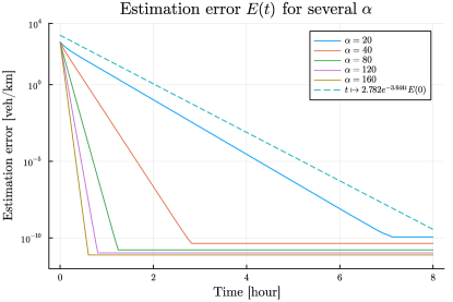
Figure 2: This figure verifies numerical values in Table 2 for the initial values $\xi\coloneqq(c,c,c),\;\hat{\xi}\coloneqq(0,0,0)$ and the input function $u(t)\coloneqq(\alpha,c-\alpha)$, $t\geq 0$. The vertical axis is logarithmic and the dashed line corresponds with the function $t\mapsto 2.782\cdot e^{-3.644t}E(0)$ where $3.644$ is the largest $\lambda$ in Table 2 and $2.782$ is the associated value for $\gamma$. Notice that for all $\alpha\in\{20,40,80,120,160\}$, the slope of $\log E(t)$ (which eventually stagnates due to machine precision) is steeper than the dashed line. This suggests (in this particular case) that the values for $\lambda$ in Table 2 are conservative.

To put Table 2 into further perspective, consider the number $L_{a}\coloneqq-\log(a/\gamma)/\lambda$ for $a\in(0,1)$, then

$$\gamma e^{-\lambda(t-\tau_{0})}\leq a,\text{ if }t\geq\tau_{0}+L_{a}.$$ (77)

If the assumption (LABEL:eq:boundary-criterion) is satisfied with $\tau_{1}-\tau_{0}\geq L_{a}$, then

$$E(t)\leq aE(t_{0}),\quad t\geq\tau_{1}.$$ (78)

For $a\coloneqq 0.5$ and $\alpha\coloneqq 40$ with the corresponding $\lambda$, $\gamma$ in Table 2, we get

$$L_{0.5}=-\frac{1}{0.332}\log(1.49/0.5)=2.76.$$ (79)

Meaning: if the traffic density in road segment $x_{0}$ is bounded from below by $40$ veh/km for $2.76$ hours, then the estimation error has at least halved when $2.76$ hours have passed. The same holds if the traffic density in $x_{n+1}$ is bounded from above by $c-\alpha=160$ veh/km during an interval of the same length. In Table 3, $L_{a}$ is computed for several $\alpha$ and $a$.

Table 3: Numerical value of $L_{a}\coloneqq-\log(a/\gamma)/\lambda$ with the $\lambda$, $\gamma$ in table 2.

$\alpha$	$L_{0.9}$	$L_{0.8}$	$L_{0.5}$	$L_{0.3}$	$L_{0.2}$
20	4.06	6.48	16.14	26.63	34.95
40	1.03	1.41	2.93	4.59	5.9
80	0.4	0.47	0.78	1.11	1.38
120	0.33	0.37	0.55	0.74	0.89
160	0.31	0.34	0.47	0.61	0.72

Remark 4.6 (Comparing 1 and 2).

1 guarantees $E(t)\leq\gamma e^{-\lambda t}E(0)$ for all $t\geq 0$. Provided that the road segment $x_{0}$ is bounded from below by $\alpha>0$ veh/km for all $t\geq 0$ or that $x_{n+1}(t)<c-\alpha$ for all $t\geq 0$. This is of course an unrealistic assumption because no road segment is neither forever non-empty nor forever non-full. It is more reasonable to assume that it is a recurring event that for some sufficiently large interval $I$ either: $x_{0}(t)\geq\alpha$ for all $t\in I$, $x_{n+1}(t)\leq c-\alpha$ for all $t\in I$, or both. Table 2 gives us an estimate of how much $E(t)$ decreases throughout these events according to their length and the value of $\alpha$. This renders 2 more relevant for traffic density estimation if modelled by (F).

So far we have computed the estimation error $E(t)$ for $n=3$ and $u$ a constant function. As $n$ increases the estimate of $\lambda$ approaches zero quite fast. Nevertheless, exponential convergence of $E(t)$ is guaranteed if the assumption (LABEL:eq:boundary-criterion) is satisfied for $\tau_{0}=0$ and all $\tau_{1}\geq 0$. And this for any $n\geq 2$. In Fig 3 we confirm that this is indeed the case for $n\in\{30,40,50,60\}$ and the input function $u$ given by

$$u_{1}(t)\coloneqq 80+20\big{(}1+\cos(\frac{2\pi}{24}t)\big{)},\quad u_{2}(t)\coloneqq c-u_{1}(t)$$ (80)

and the initial values $\xi=(0,\dots,0)$ and $\hat{\xi}=(c,\dots,c)$. This wraps up the numerical experiments.

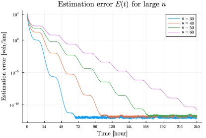
Figure 3: The estimation error $E(t)$ on a logarithmic scale for $n\in\{30,40,50,60\}$, $c\coloneqq 200$ and $w\coloneqq 0.55$, initial values $\xi\coloneqq(0,\dots,0)$ and $\hat{\xi}\coloneqq(c,\dots,c)$, and the input function $u$ given in (80). The graphs stagnate due to machine precision.

5 Conclusion

Incremental stability was considered for the UFM. In the main result Theorem 3.3, appropriate conditions related to (F) being inflow-connected and outflow-connected were given, such that any two solutions to the UFM approach each other at an exponential rate. Two corollaries followed from the main theorem. 1 shows that the UFM is IES in the whole state space with respect to an appropriate set of input functions. And 2 shows that under milder conditions compared with the latter, all solutions to the UFM converge to each other asymptotically. In the numerical experiments, the results were applied to estimate traffic density in a hypothetical highway. The exponential rate in the main theorem was computed numerically and tested against simulations of the UFM, which suggested the exponential rate to be conservative.

Possible future research directions include but are not limited to showing incremental stability for UFM-like models with e.g. alternative flow functions or connections between the compartments. To investigate control applications related to incremental stability of the UFM is also recommended.

Proposition 3.

For all $(\xi,u)\in C\times U$, system (F) admits a unique solution $x$, such that $x(0)=\xi$, $x(t)$ is defined for all $t\geq 0$, and

$$x(t)\in C\text{ for all $t\geq 0$.}$$ (81)

Proof .7.

Let $h>0$, $u\in U$, and $\xi\in C$ be arbitrary but fixed. Define $D\coloneqq(-h,+\infty)\times(-h,c+h)^{n}\subset\mathbb{R}^{n+1}$ and

$$\begin{split}\partial D\coloneqq\Big{\{}&(t,x)\in\bar{D}\;:\;t\in\{-h,+\infty\}\\ &\text{ or }x_{j}\in\{-h,c+h\}\text{ for some $j\in\{1,\dots,n\}$}\Big{\}},\end{split}$$

where $\partial D$ and $\bar{D}$ are the boundary and closure of $D$, respectively. Let $b\coloneqq(c/2,\dots,c/2)\in\mathbb{R}^{n}$, and $F_{u}^{k}:D\to\mathbb{R}^{n}$ be defined as

$$F_{u}^{k}(t,y)\coloneqq\begin{cases}f(y,u(t)),\quad k=0,\\ f(y,u(t))+(b-y)/k,\quad k\in\mathbb{N},\end{cases}$$ (82)

where $f$ is defined in (11). Taking inspiration from [5, pg. 127], consider the auxiliary initial value problems given by

$$\dot{x}^{k}(t)=F_{u}^{k}(t,x(t)),\quad x^{k}(0)=\xi.$$ (83)

Note that when $k=0$, the differential equation given in (83) is the same as (F). In other words, if (F) admits a unique solution so that $x(0)=\xi$, then $x^{0}=x$. Our goal is to show that for $k=0$, (83) admits a unique solution defined for all $t\geq 0$ such that

$$x^{0}(t)\in C\text{ for all }t\geq 0.$$ (84)

We will now show that (83) admits a unique local solution for all $k\geq 0$. Fix any $k\geq 0$. The map $F_{u}^{k}(t,y)$ is continuous in $t$ and polynomial in $y$ on the whole domain $D$. Therefore, the Jacobian $\partial F_{u}^{k}(t,y)/\partial y$ exists, is continuous for all $(t,y)\in D$, and $F_{u}^{k}(t,y)$ is locally Lipschitz with respect to $y$ in $D$. Since the initial data $(0,\xi)\in\{0\}\times C\subset D$ and $F_{u}^{k}$ is locally Lipschitz, we can invoke Theorem 3.1 in [11, pg. 18] to confirm that (83) admits a unique, continuously differentiable solution, defined locally around $t=0$.

Let $D_{x^{k}}$ denote the maximum interval of existence for $x^{k}$ and $\beta_{k}\coloneqq\sup D_{x^{k}}$. Since $D$ is an open set, $F_{u}^{k}$ is continuous and $(0,\xi)\in D$, it follows from Theorem 2.1 in [11, pg. 17] that $(t,x^{k}(t))$ tends to the boundary of $D$ as $t\to\beta_{k}$. Suppose $x^{k}(t)\in C$ for all $t\in[0,\beta_{k})$, then $\beta_{k}=+\infty$. If not, then $(t,x^{k}(t))$ would not approach the boundary of $D$ as $t\to\beta_{k}$.

Our intermediate goal is to prove (by contradiction) the following claim:

$$x^{k}(t)\in C\text{ for all }t\in[0,\beta_{k})\text{ and for all }k\geq 1.$$ (85)

Let $k\geq 1$ be arbitrary but fixed and define

$$T\coloneqq\inf\{t\in[0,\beta_{k})\;:\;x^{k}(t)\not\in C\}.$$ (86)

We will show that $T=\beta_{k}$. If $T<\beta_{k}$ then $x^{k}(T)$ is defined and

$$x(T)\in C=[0,c]^{n},$$ (87)

since $x^{k}$ is continuous and $C$ is compact. It further follows from $T<\beta_{k}$, that there exists an index $j\in\{1,\dots,n\}$ and small $\delta>0$ so that exactly one of the following cases is true:

$$x_{j}^{k}(T) =c\text{ and }x_{j}^{k}(t)>c\text{ for all }t\in(T,T+\delta),$$ (88a)

$$x_{j}^{k}(T) =0\text{ and }x_{j}^{k}(t)<0\text{ for all }t\in(T,T+\delta),$$ (88b)

which follows by definition of $T$ and continuity of $x^{k}$. In addition, since $x^{k}$ is continuously differentiable, (88a) and (88b) imply

$$x^{k}_{j}(T) =c\text{ and }\dot{x}^{k}_{j}(T)\geq 0,$$ (89a)

$$x^{k}_{j}(T) =0\text{ and }\dot{x}^{k}_{j}(T)\leq 0,$$ (89b)

respectively. For convenience we explicitly write each component of $F_{u}^{k}(t,y)$ for $k\geq 1$

$$\begin{split}(F_{u}^{k}(t,y))_{1}&=wu_{1}(t)(c-y_{1})-wy_{1}(c-y_{2})\!+\!\frac{c/2-y_{1}}{k}\\ (F_{u}^{k}(t,y))_{j}&=wy_{j-1}(c-y_{j})-wy_{j}(c-y_{j+1})\!+\!\frac{c/2-y_{j}}{k},\\ (F_{u}^{k}(t,y))_{n}&=wy_{n-1}(c-y_{n})-wy_{n}(c-u_{2}(t))\!+\!\frac{c/2-y_{n}}{k},\end{split}$$

where $j=2,\dots,n-1$. Recall also that $u:\mathbb{R}\to[0,c]^{2}$ and $c,w>0$. Suppose $x_{j}^{k}(T)=c$, then

$$\begin{split}\dot{x}^{k}_{j}(T)&=(F_{u}^{k}(T,x^{k}(T)))_{j}\\ &=-wc(c-x^{k}_{j+1}(T))-\frac{c}{2k}\\ &\leq-\frac{c}{2k}<0,\end{split}$$ (90)

where we use $x^{k}_{j}(T)\in[0,c]$ for the first inequality. If $j=n$, we interpret $x^{k}_{n+1}(T)$ as $u_{2}(T)$ which takes a value in $[0,c]$. On the other hand, if $x_{j}^{k}(T)=0$, then

$$\begin{split}\dot{x}^{k}_{j}(T)&=(F_{u}^{k}(T,x^{k}(T)))_{j}\\ &=wx^{k}_{j-1}(T)c+\frac{c}{2k}\\ &\geq\frac{c}{2k}>0,\end{split}$$ (91)

where we use $x_{j-1}^{k}(T)\in[0,c]$ in the first inequality. If $j=1$, we interpret $x_{0}^{k}(T)$ as $u_{1}(T)$ which takes a value in $[0,c]$. Indeed, the strict inequalities in (90) and (91) contradict (89a) and (89b), respectively. Therefore $x^{k}$ remains in $C$ and $T=\beta_{k}$. The claim in (85) has thus been proven and we conclude in addition that $\beta_{k}=+\infty$ for all $k\geq 1$.

Next we prove that $F_{u}^{k}(t,y)$ converges uniformly to $F_{u}^{0}(t,y)$ on compact subsets of $D$ as $k\to+\infty$. Let $K_{t}\subset(-h,+\infty)$ be a closed interval, $K_{y}\subset(-h,h+c)^{n}$ compact, and $K\coloneqq K_{t}\times K_{y}$ an arbitrary compact subset of $D$. Since $K_{y}$ is compact, there exists $\gamma\geq 0$ such that $|b-y|_{1}\leq\gamma$ for all $y\in K_{y}$. For all $(t,y)\in K$

$$\begin{split}|F_{u}^{0}(t,y)-F_{u}^{k}(t,y)|_{1}&=|(b-y)/k|_{1}\\ &=\frac{1}{k}\sum_{i=1}^{n}|\frac{c}{2}-y_{i}|\\ &\leq\frac{\gamma}{k}.\end{split}$$ (92)

For each $\epsilon>0$ there exists $k_{\epsilon}\geq 1$ such that $\gamma/k\leq\epsilon$ for all $k\geq k_{\epsilon}$, which proves that $F_{u}^{k}(t,y)\to F_{u}^{0}(t,y)$ uniformly on $K$ as $k\to+\infty$.

We can now prove that

$$x^{0}(t)\in C\text{ for all }t\in[0,\beta_{0}).$$ (93)

Suppose there exists $\tau\in[0,\beta_{0})$ so that $x^{0}(\tau)\not\in C$. Then there exists $j\in\{1,\dots,n\}$ so that $x_{j}(\tau)\in(-h,0)\cup(c,c+h)$. Let $\Pi_{0}=[0,\pi_{0}]$ where $\pi_{0}\in(\tau,\beta_{0})$. We showed earlier in the proof that for all $k\geq 1$, $x^{k}$ is defined on $[0,+\infty)$ and therefore defined on $\Pi_{0}$ as well. Since $F_{u}^{k}\to F_{u}^{0}$ uniformly on compact subsets of $D$, as $k\to+\infty$, it holds by virtue of Lemma 3.1 in [11, pg. 24] that

$$\lim_{k\to+\infty}\sup_{t\in\Pi_{0}}|x^{k}(t)-x(t)|_{1}=0.$$ (94)

The limit in (94) implies that $x^{0}(t)\in C$ for all $t\in\Pi_{0}$. If this is not true, consider the following lower-bound

$$\begin{split}\lim_{k\to+\infty}\sup_{t\in\Pi_{0}}|x^{k}(t)-x^{0}(t)|_{1}&\geq\lim_{k\to+\infty}|x^{k}(\tau)-x^{0}(\tau)|_{1}\\ &\geq\lim_{k\to+\infty}|x_{j}^{k}(\tau)-x_{j}(\tau)|,\end{split}$$ (95)

which becomes strictly larger than $0$, if $x_{j}^{0}(\tau)\not\in[0,c]$, since $x_{j}^{k}(\tau)\in[0,c]$ for all $k\geq 1$. We have now shown (93) and we conclude that $\beta_{0}=+\infty$. Because $x=x^{0}$, the proof is complete.

Proposition 4.

System (F) is cooperative for inputs in $U$.

Proof .8.

The proof of this proposition follows directly from the developments in [24]. Let $G\coloneqq(0,c)^{n}$ and let  $F_{u}:\mathbb{R}\times\mathbb{R}^{n}\to\mathbb{R}^{n}$ be defined by $F_{u}(t,y)\coloneqq f(y,u(t))$ for some fixed but arbitrary $u\in U$. Furthermore let $\xi,\eta\in C$ with $\xi\leq\eta$ be fixed but arbitrary. We want to show that

$$\phi(t,\xi,u)\leq\phi(t,\eta,u)\text{ for all }t\geq 0.$$ (96)

Recall the definitions of the relations $\leq$ and $<$ for vectors in the end of Section 1. The function $F_{u}$ is said to be type-K in $G$ if for all $i\in\{1,\dots,n\}$ and all $s\geq 0$

$$(F_{u}(s,a))_{i}\leq(F_{u}(s,b))_{i}$$ (97)

whenever $a,b\in G$ satisfy $a\leq b$ and $a_{i}=b_{i}$.

Three conditions must be met to prove that (96) holds (see Proposition 1.1, Remark 1.2 and 1.4 in [24, ch. 3]). Firstly, it is required that $C$ is positively invariant. Meaning, any solution to (F) that begins in $C$, remains in $C$. This has already been proven in Proposition 3. Secondly, there must exist sequences $\{\xi^{k}\}_{k=1}^{+\infty}$ and $\{\eta^{k}_{k}\}_{k=1}^{+\infty}$ such that $\xi^{k},\eta^{k}\in G$ and $\xi^{k}<\eta^{k}$ for all $k\geq 1$ and that $\xi^{k}\to\xi$ and $\eta^{k}\to\eta$ as $k\to+\infty$. Since $C$ is convex this is the case (see remark III.1 in [2]). And lastly, $F_{u}$ must be type-K in $G$, which remains to be shown.

Let $i\in\{1,\dots,n\}$, $s\geq 0$, and $a,b\in G$ with $b\leq a$ and $b_{i}=a_{i}$ be fixed and arbitrary. We will show (97), by confirming that the $\delta_{i}\coloneqq(F_{u}(s,a)-F_{u}(s,b))_{i}\leq 0$. Recall that the model parameter $\omega>0$. If $i=1$,

$$\delta_{1}=-wa_{1}(b_{2}-a_{2})\leq 0.$$ (98)

If $i\in\{2,\dots,n-1\}$,

$$\delta_{i}=-w(c-a_{i})(b_{i-1}-a_{i-1})-wa_{i}(b_{i+1}-a_{i+1})\leq 0$$ (99)

And if $i=n$,

$$\delta_{n}=-w(c-a_{n})(b_{n-1}-a_{n-1})\leq 0.$$ (100)

Hence, $F_{u}$ is type-K in $G$, which completes the proof.

Proposition 5.

Consider the mapping $T:C\to C$, defined by

$$T_{i}(x)\coloneqq c-x_{n+1-i},\quad i=1,\dots,n.$$ (101)

Consider system (F) and fix any $(\xi,u)\in C\times U$. Then for all $t\geq 0$

$$\phi(t,\xi,u)=T(\phi(t,\eta,v)),$$ (102)

where $\eta=T(\xi)\in C$ and $v=(c-u_{2},c-u_{1})\in U$.

Proof .9.

Let $x_{0}\coloneqq u_{1},x_{n+1}\coloneqq u_{2}$ and $x(t)\coloneqq\phi(t,\xi,u)$. Since $x$ solves (F), we have

$$\begin{split}\dot{x}_{n+1-i}(t)=&wx_{n-i}(t)(c-x_{n+1-i}(t))\\ &-wx_{n+1-i}(t)(c-x_{n+2-i}(t))\end{split}$$ (103)

for all $i\in\{1,\dots,n\}$ and $t\geq 0$. Let then $y(t)\coloneqq T(x(t))$ for $t\geq 0$ and take $y_{0}\coloneqq c-x_{n+1}$ and $y_{n+1}\coloneqq c-x_{0}$. Using (103), the definition of the $y_{i}$, and the fact that $\dot{y}_{i}=-\dot{x}_{n+1-i}$, we obtain

$$\begin{split}\dot{y}_{i}(t)&=wy_{i-1}(t)(c-y_{i}(t))-wy_{i}(t)(c-y_{i+1}(t)).\end{split}$$ (104)

for all $i\in\{1,\dots,n\}$ and $t\geq 0$ Note that $y_{0}=c-u_{2}=v_{1}$, $y_{n+1}=c-u_{1}=v_{2}$, and $y(0)=T(x(0))=T(\xi)\in C$. It follows from the definition of $T$ that $T(\xi)\in C$ since $\xi\in C$. And it follows from the definition of $U$ in (10) that $v=(c-u_{2},c-u_{1})\in U$, since $u\in U$. Comparing the right-hand side of (104) with the definition of $f$ in (11), we conclude that $y$ solves (F) with the input function $v$ and initial value $\eta=T(\xi)$. Since $T$ is invertible and $T=T^{-1}$, $x(t)=T(y(t))$ for all $t\geq 0$, which shows that (102) is true since $x(t)=\phi(t,\xi,u)$ and $y(t)=\phi(t,\eta,v)$. This completes the proof.

Proof of Lemma 3.2: By the assumptions $s\in(0,c)^{n}\times(0,c]$ and $\sigma>1$, and the definitions (37)-(39) it holds that $q$, $v$, and $\omega$ are elements of $(0,+\infty)^{n}$. To show (41), consider the ordering

$$|q|_{1}=\omega_{1}>\dots>\omega_{n}=q_{n},$$ (105)

which follows by (39) and $q\in(0,+\infty)^{n}$. Hence, $q_{n}\leq\omega_{i}\leq|q|_{1}$ for all $i\in\{1,\dots,n\}$, which implies

$$q_{n}\sum_{i=1}^{n}x_{i}\leq\sum_{i=1}^{n}\omega_{i}x_{i}\leq|q|_{1}\sum_{i=1}^{n}x_{i},\quad x\in[0,+\infty)^{n}.$$ (106)

For all $x\in[0,+\infty)^{n}$, $|x|_{1}=\sum_{i=1}^{n}x_{i}$. The inequalities (41) have thus been shown, because $V(x)=\sum_{i=1}^{n}\omega_{i}x_{i}$.

We move on to prove (43). Fix any $u\in[0,c]\times[0,s_{n+1}]$ and $x,y\in[0,c-s_{1}]\times\dots\times[0,c-s_{n}]$ with $y\leq x$. Moreover, define $W\coloneqq\langle\omega,f(x,u)-f(y,u)\rangle$, $p\coloneqq f(x,u)-f(y,u)$ and $\delta\coloneqq x-y$. If

$$W\leq-\lambda V(\delta),$$ (107)

then the proof is complete. Recall the definition (39) of $\omega$, which we use to write

$$\begin{split}W=\sum_{i=1}^{n}p_{i}\sum_{k=i}^{n}q_{k}=\sum_{k=1}^{n}q_{k}\sum_{i=1}^{k}p_{i}.\end{split}$$ (108)

Let $M_{k}\coloneqq\sum_{i=1}^{k}p_{i}$. Using the definition of $f$ in (11) we obtain the expressions

$$\begin{split}M_{n}=&-wu_{1}\delta_{1}-w\delta_{n}(c-u_{2}),\text{ and }\\ M_{k}=&-wu_{1}\delta_{1}-wx_{k}(c-x_{k+1})+wy_{k}(c-y_{k+1}),\;\;k\neq n.\end{split}$$

Substituting $\sum_{i=1}^{k}p_{i}$ by the expression for $M_{1},\dots,M_{n}$ into (108) yields

$$\begin{split}W=&\sum_{k=1}^{n}q_{k}M_{k}\\ =&-w|q|_{1}u_{1}\delta_{1}-wq_{n}\delta_{n}(c-u_{2})\\ &+w\sum_{i=1}^{n-1}q_{i}\big{(}y_{i}\delta_{i+1}-(c-x_{i+1})\delta_{i}\big{)},\end{split}$$ (109)

where we use the equality $y_{i}(c-y_{i+1})-x_{i}(c-x_{i+1})=y_{i}\delta_{i+1}-(c-x_{i+1})\delta_{i}$, $i\neq n$. Recall that $w>0$ and $\delta\coloneqq x-y\in[0,+\infty)^{n}$. We upper bound $W$ as follows

$$\begin{split}W\leq&w\sum_{i=1}^{n-1}q_{i}\big{(}y_{i}\delta_{i+1}-(c-x_{i+1})\delta_{i}\big{)}\\ &-wq_{n}\delta_{n}(c-u_{2})\\ \leq&w\sum_{i=1}^{n-1}q_{i}\big{(}(c-s_{i})\delta_{i+1}-s_{i+1}\delta_{i}\big{)}\\ &-wq_{n}s_{n+1}\delta_{n},\end{split}$$ (110)

where we add $|q|_{1}u_{1}\delta_{1}\geq 0$ to the right hand side of (109) in the first step. In the second step, we use $x_{i},y_{i}\in[0,c-s_{i}]$ and $u_{2}\in[0,c-s_{n+1}]$. By definition of $q$, $v$ in (37), (38) we have the relation

$$v_{i}=q_{i}s_{i+1}-q_{i-1}(c-s_{i-1}),\quad i=2,\dots,n.$$ (111)

Using this relation and the fact that $v_{1}\coloneqq q_{1}s_{2}$, we rewrite (110) to get

$$\begin{split}W&\leq w\sum_{i=1}^{n-1}q_{i}(c-s_{i})\delta_{i+1}-w\sum_{i=1}^{n}q_{i}s_{i+1}\delta_{i}\\ &=w\sum_{i=2}^{n}q_{i-1}(c-s_{i-1})\delta_{i}-w\sum_{i=1}^{n}q_{i}s_{i+1}\delta_{i}\\ &=-wq_{1}s_{2}\delta_{1}-w\sum_{i=2}^{n}\big{(}q_{i}s_{i+1}-q_{i-1}(c-s_{i-1})\big{)}\delta_{i}\\ &=-w\sum_{i=1}^{n}v_{i}\delta_{i}.\end{split}$$ (112)

Since $\delta\in[0,+\infty)^{n}$, we can apply the inequality (106) to get

$$\sum_{i=1}^{n}\delta_{i}\geq\frac{1}{|q|_{1}}\sum_{i=1}^{n}\omega_{i}\delta_{i}=\frac{1}{|q|_{1}}\langle\omega,\delta\rangle.$$ (113)

Finally, we have

$$\begin{split}W&\leq-w\min_{i}\{v_{i}\}\sum_{i=1}^{n}\delta_{i}\\ &\leq-w\frac{\min_{i}\{v_{i}\}}{|q|_{1}}\sum_{i=1}^{n}\omega_{i}\delta_{i}=-\lambda\langle\omega,\delta\rangle,\end{split}$$ (114)

where we use $v\in(0,+\infty)^{n}$, $\delta\in[0,+\infty)^{n}$, and (112) in the first step; (113) in the second; and $\lambda\coloneqq w\min\{v_{i}\}/|q|_{1}$ in the last. The inequality (107) has thus been shown, since $V(\delta)=\langle\omega,\delta\rangle$, which completes the proof.

References

- [1] D. Angeli “A Lyapunov approach to incremental stability properties” In IEEE Transactions on Automatic Control 47.3, 2002, pp. 410–421
- [2] D. Angeli and E.D. Sontag “Monotone control systems” In IEEE Transactions on Automatic Control 48.10, 2003, pp. 1684–1698
- [3] G. Aronsson and R.B. Kellogg “On a differential equation arising from compartmental analysis” In Mathematical Biosciences 38.1-2, 1978, pp. 113–122
- [4] R. N. Bergman “Toward Physiological Understanding of Glucose Tolerance: Minimal-Model Approach” In Diabetes 38.12, 1989, pp. 1512–1527
- [5] F. Blanchini and Stefano Miani “Set-theoretic methods in control” Springer, 2008
- [6] F. Blanchini et al. “Optimal control of compartmental models: The exact solution” In Automatica 147, 2023, pp. 110680
- [7] S. Coogan “A contractive approach to separable Lyapunov functions for monotone systems” In Automatica 106, 2019, pp. 349–357
- [8] C.F. Daganzo “The cell transmission model: A dynamic representation of highway traffic consistent with the hydrodynamic theory” In Transportation Research Part B: Methodological 28.4, 1994, pp. 269–287
- [9] G. Dirr, H. Ito, A. Rantzer and B. Ruffer “Separable Lyapunov functions for monotone systems: Constructions and limitations” In Discrete Contin. Dyn. Syst. Ser. B 20.8, 2015, pp. 2497–2526
- [10] J. Eisenfeld “On washout in nonlinear compartmental systems” In Mathematical Biosciences 58.2, 1982, pp. 259–275
- [11] J.K. Hale “Ordinary Differential Equations”, Dover Books on Mathematics Series Dover Publications, 2009
- [12] J. A. Jacquez and C. P. Simon “Qualitative theory of compartmental systems” In Siam Review 35.1, 1993, pp. 43–79
- [13] Y. Kawano, B. Besselink and M Cao “Contraction Analysis of Monotone Systems via Separable Functions” In IEEE Transactions on Automatic Control 65.8, 2020, pp. 3486–3501
- [14] A. Lajmanovich and J. A. Yorke “A deterministic model for gonorrhea in a nonhomogeneous population” In Mathematical Biosciences 28.3-4, 1976, pp. 221–236
- [15] M. Y. Li and J. S. Muldowney “Global stability for the SEIR model in epidemiology” In Mathematical Biosciences 125.2, 1995, pp. 155–164
- [16] W. Lohmiller and J-J. E. Slotine “On contraction analysis for non-linear systems” In Automatica 34.6, 1998, pp. 683–696
- [17] H. Maeda, S. Kodama and Y. Ohta “Asymptotic behavior of nonlinear compartmental systems: Nonoscillation and stability” In IEEE Transactions on Circuits and Systems 25.6, 1978, pp. 372–378
- [18] M. Margaliot, Sontag E.D. and Tuller T. “Contraction after small transients” In Automatica 67, 2016, pp. 178–184
- [19] M. Margaliot and T. Tuller “Stability Analysis of the Ribosome Flow Model” In IEEE/ACM Transactions on Computational Biology and Bioinformatics 9.5, 2012, pp. 1545–1552
- [20] M. Pereira, A. Lang and B. Kulcsar “Short-term traffic prediction using physics-aware neural networks” In Transportation research part C: emerging technologies 142, 2022, pp. 103772
- [21] M. Pereira, P. B. Baykas, B. Kulcsár and A. Lang “Parameter and density estimation from real-world traffic data: A kinetic compartmental approach” In Transportation Research Part B: Methodological 155, 2022, pp. 210–239
- [22] M. Pereira et al. “The Traffic Reaction Model: A kinetic compartmental approach to road traffic modeling” In Transportation Research Part C - Emerging Technology (to appear), 2024
- [23] I. Sandberg “On the mathematical foundations of compartmental analysis in biology, medicine, and ecology” In IEEE transactions on Circuits and Systems 25.5, 1978, pp. 273–279
- [24] H. L. Smith “Monotone dynamical systems: an introduction to the theory of competitive and cooperative systems” American Mathematical Soc., 2008
- [25] J.M. Van Den Hof “Positive linear observers for linear compartmental systems” In SIAM Journal on Control and Optimization 36.2, 1998, pp. 590–608
- [26] G.G. Walter and M. Contreras “Compartmental modeling with networks” Springer Science & Business Media, 1999
- [27] Y. Zarai, M. Margaliot and T. Tuller “Ribosome flow model with extended objects” In Journal of The Royal Society Interface 14.135, 2017, pp. 20170128